T6D-Direct: Transformers for Multi-Object
6D Pose Direct Regression

Abstract

6D pose estimation is the task of predicting the translation and orientation of objects in a given input image, which is a crucial prerequisite for many robotics and augmented reality applications. Lately, the Transformer Network architecture, equipped with multi-head self-attention mechanism, is emerging to achieve state-of-the-art results in many computer vision tasks. DETR, a Transformer-based model, formulated object detection as a set prediction problem and achieved impressive results without standard components like region of interest pooling, non-maximal suppression, and bounding box proposals. In this work, we propose T6D-Direct, a real-time single-stage direct method with a transformer-based architecture built on DETR to perform 6D multi-object pose direct estimation. We evaluate the performance of our method on the YCB-Video dataset. Our method achieves the fastest inference time, and the pose estimation accuracy is comparable to state-of-the-art methods.

1 Introduction

6D object pose estimation in clutter is a necessary prerequisite for autonomous robot manipulation tasks and augmented reality. Given the complex nature of the task, methods for object pose estimation—both traditional and modern—are multi-staged [35, 7, 26, 19]. The standard pipeline consists of an object detection and/or instance segmentation, followed by the region of interest cropping and processing the cropped patch to estimate the 6D pose of an object. Convolutional neural networks (CNNs) are the basic building blocks of the deep learning models for computer vision tasks. CNN’s strength lies in the ability to learn local spatial features. Motivated by the success of deep learning methods for computer vision, in a strive for end-to-end differentiable pipelines, many of the traditional components like non-maximum suppression (NMS) and region of interest cropping (RoI) have been replaced by their differentiable counterparts [8, 4, 24]. Despite these advancements, the pose estimation accuracy still heavily depends on the initial object detection stage.

Recently, Transformer, an architecture based on self-attention mechanism, is achieving state-of-the-art results in many natural language processing tasks. Transformers are efficient in modeling long-range dependencies in the data, which is also beneficial for many computer vision tasks. Some recent works achieved state-of-the-art results in computer vision tasks using the Transformer architecture to supplement CNNs or to completely replace CNNs  [3, 30, 1, 37, 34, 12].

Carion et al. introduced DETR [1], an object detection pipeline using Transformer in combination with a CNN backbone model and achieved impressive results. DETR is a simple architecture without any handcrafted procedures like NMS and anchor generation. It formulates object detection as a set prediction problem and uses bipartite matching and Hungarian loss to implement an end-to-end differentiable pipeline for object detection.

In this paper, we present T6D-Direct, an extension to the DETR architecture to perform multi-object 6D pose direct regression in real-time. T6D-Direct enables truly end-to-end pipeline for 6D object pose estimation where the accuracy of the pose estimation is not reliant on object detection and the subsequent cropping. In contrast to the standard methods of 6D object pose estimation that are multi-staged, our method is direct single-stage and estimates the pose of all the objects in a given image in one forward pass. In short, our contributions include:

1. An elegant real-time end-to-end differentiable architecture for multi-object 6D pose direct regression.

2. Evaluation of different design choices for implementing multi-object 6D pose direct regression as a set prediction problem.

2 Related Work

In this section, we review the state-of-the-art methods for 6D object pose estimation and DETR, the transformer architecture our proposed method is based on, in detail.

2.1 Pose Estimation

Like most other computer vision tasks, the state-of-the-art methods for 6D object pose estimation from RGB images are predominantly convolutional neural network (CNN)-based. The standard CNN architectures for object pose estimation are multi-staged. The first stage is object detection and/or instance segmentation. In the second stage, using the object bounding boxes, predicted an image patch containing the target object, is extracted and the 6D pose of the object is estimated. The common methods for object pose estimation can be broadly classified into three categories: direct, indirect, and refinement-based.

Direct methods regress for the translation and orientation components of the object pose directly from the RGB images [35, 21, 9].  Kehl et al. [11], Sundermeyer et al. [28] discretized the orientation component of the 6D pose and performed classification instead of regression.

Indirect approaches aim to recover the 6D pose from the 2D-3D correspondences using the PnP algorithm, where PnP is often used in combination with the RANSAC algorithm to increase the robustness against outliers in correspondence prediction  [23, 29, 10, 20]. Although indirect methods outperform direct methods in the recent benchmarks [7], indirect models are significantly larger, and the model size grows exponentially with the number of objects. One common solution to keep the model size small is to train one lighter model for each object. This approach, however, introduces significant overhead for many real-world applications. Direct models, on the other hand, are lighter, and their end-to-end differentiable nature is desirable in many applications [32].  Wang et al. [33], Li et al. [15] unified direct regression and dense estimation methods by introducing a learnable PnP module.

Refinement-based methods formulate 6D pose estimation as an iterative refinement problem where in each step given the observed image and the rendered image according to the current pose estimate, the model predicts a pose update that aligns the observed and the rendered image better. The process is repeated until the estimated pose update is negligibly small. Refinement-based methods are orthogonal to the direct and indirect methods and are often used in combination with these methods [13, 18, 27, 22, 14], i.e., direct or indirect methods produce initial pose estimate and the refinement-based methods are used to refine the initial pose estimate to predict the final accurate pose estimate.

2.2 DETR

Carion et al. [1] introduced DETR, an end-to-end differentiable object detection model using the Transformer architecture. They formulated object detection, the problem of estimating the bounding boxes and class label probabilities, as a set prediction problem. Given an RGB input image, the DETR model outputs a set of tuples with fixed cardinality. Each tuple consists of the bounding box and class label probability of an object. To allow an output set with a fixed cardinality, a larger cardinality is chosen, and a special class id Ø is used for padding the rest of the tuples in addition to the actual object detections. The tuples in the predicted set and the ground truth target set are matched by bipartite matching using the Hungarian algorithm. The DETR model achieved competitive results on the COCO dataset [16] compared to standard CNN-based architectures.

3 Method

Figure 1: T6D-Direct overview. Given an RGB image, we use a CNN backbone to extract lower-resolution image features and flatten them to create feature vectors suitable for a standard Transformer model. The Transformer model generates a set of predictions with a fixed cardinality $N$. To facilitate the prediction of a varying number of objects in an image, we choose $N$ to be much larger than the expected number of objects in an image and pad the rest of the tuples in the set with Ø object predictions. We perform bipartite matching between the predicted and ground truth sets to find the matching pairs and train the pipeline to minimize the Hungarian loss between the matched pairs.

In this section, we describe our approach of formulating 6D object pose estimation as a set prediction problem and describe the extensions we made to the DETR model and the bipartite matching process to enable the prediction of a set of tuples of bounding boxes, class label probabilities, and 6D object poses. Fig. 1 provides an overview of the proposed T6D-Direct model.

3.1 Pose Estimation as Set Prediction

Inspired by the DETR model, we formulate 6D object pose direct regression as a set prediction problem. We call our method T6D-Direct. In the following sections, we describe the individual components of the T6D-Direct model in detail.

3.1.1 Set Prediction

Given an RGB input image, our model generates a set of tuples. Each tuple consists of a bounding box, represented as center coordinates, height and width, class label probabilities, translation and orientation components of the 6D object pose. The height and width of the bounding boxes are proportional to the size of the image. For the orientation component, we opt for the 6D continuous representation as shown to yield the best performance in practice [36]. To facilitate the 6D pose prediction of a varying number of objects in an image, we fix the cardinality of the predicted set to $N$, which is a hyperparameter, and we chose it to be larger than the expected maximum number of objects in the image. In this way, the network has enough options to embed each object freely. The T6D-Direct model is trained to predict the tuples corresponding to the objects in the image and predict Ø class to pad the rest of the tuples in the fixed size set.

3.1.2 Bipartite Matching

Given $n$ ground truth objects ${y}_{1},{y}_{2},...,{y}_{n}$, we pad Ø objects to create a ground truth set $y$ of cardinality $N$. To match the predicted set $\hat{y}$, generated by our T6D-Direct model, with the ground truth set $y$, we perform bipartite matching. Formally, we search for the permutation of elements between the two sets $\sigma\in\mathfrak{S}_{N}$ that minimizes the matching cost:

$$\hat{\sigma}=\operatorname*{arg\,min}_{\sigma\in\mathfrak{S}_{N}}\sum_{i}^{N}\mathcal{L}_{match}(y_{i},\hat{y}_{\sigma(i)}),$$ (1)

where $\mathcal{L}_{match}(y_{i},\hat{y}_{\sigma(i)})$ is the pair-wise matching cost between the ground truth tuple $y_{i}$ and the prediction at index $\sigma(i)$. DETR model included bounding boxes $b_{i}$ and class probabilities $p_{i}$ in their cost function. In the case of T6D-Direct model, we have two options for defining $\mathcal{L}_{match}(y_{i},\hat{y}_{\sigma(i)})$. One option is to use the same definition used by the DETR model, i.e., we include only bounding boxes and class probabilities and ignore pose predictions in the matching cost. We call this variant of matching cost as $\mathcal{L}_{match\_object}$.

$$\mathcal{L}_{match\_object}(y_{i},\hat{y}_{\sigma(i)})=-\mathbbm{1}_{c_{i}\neq\text{\O}}\hat{p}_{\sigma(i)}(c_{i})+\mathbbm{1}_{c_{i}\neq\text{\O}}\mathcal{L}_{box}(b_{i},\hat{b}_{\sigma(i)}).$$ (2)

The second option is to include the pose predictions in the matching cost as well. We call this variant $\mathcal{L}_{match\_pose}$.

$$\mathcal{L}_{match\_pose}(y_{i},\hat{y}_{\sigma(i)})=\mathcal{L}_{match\_object}(y_{i},\hat{y}_{\sigma(i)})+\\ \mathcal{L}_{rot}(R_{i},\hat{R}_{\sigma(i)})+\mathcal{L}_{trans}(t_{i},\hat{t}_{\sigma(i)}),$$ (3)

where $\mathcal{L}_{rot}$ is the angular distance between the ground truth and predicted rotations, and $\mathcal{L}_{trans}$ is the $\ell_{2}$ loss between the ground truth and estimated translations. We experimented with both variants, and we opted for the former method.

3.1.3 Hungarian Loss

After establishing the matching pairs using the bipartite matching, the T6D-Direct model is trained to minimize the Hungarian loss between the predicted and ground truth target sets consisting of probability loss, bounding box loss, and pose loss:

$$\mathcal{L}_{Hungarian}(y,\hat{y})=\sum_{i}^{N}[-\text{log}\hat{p}_{\hat{\sigma}(i)}(c_{i})+\mathbbm{1}_{c_{i}\neq\text{\O}}\mathcal{L}_{box}(b_{i},\hat{b}_{\hat{\sigma}(i)})+\\ \lambda_{pose}\mathbbm{1}_{c_{i}\neq\text{\O}}\mathcal{L}_{pose}(R_{i},t_{i},\hat{R}_{\hat{\sigma}(i)},\hat{t}_{\hat{\sigma}(i)})].$$ (4)

3.1.4 Class probability loss

The first component in the Hungarian loss is the class probability loss. We use the standard negative log-likelihood loss as the class probabilities loss function. Additionally, the number of Ø classes in a set is significantly larger than the other object classes. To counter this class imbalance, we weight the log probability loss for the Ø class by a factor of 0.4.

3.1.5 Bounding box loss

The second component in the Hungarian loss is bounding box loss $\mathcal{L}_{box}(b_{i},\hat{b}_{\sigma(i)})$. We use a weighted combination of generalized IOU [25] and $\ell_{1}$ loss.

$$\mathcal{L}_{box}(b_{i},\hat{b}_{\sigma(i)})=\alpha\mathcal{L}_{iou}(b_{i},\hat{b}_{\sigma(i)})+\beta||b_{i}-\hat{b}_{\sigma(i)}||,$$ (5)

$$\mathcal{L}_{iou}(b_{i},\hat{b}_{\sigma(i)})=1-\left(\frac{|b_{i}\cap\hat{b}_{\sigma(i)}|}{|b_{i}\cup\hat{b}_{\sigma(i)}|}-\frac{|B(b_{i},\hat{b}_{\sigma(i)})\setminus b_{i}\cup\hat{b}_{\sigma(i)}|}{|B(b_{i},\hat{b}_{\sigma(i)})|}\right),$$ (6)

where $\alpha$, $\beta$ are hyperparameters and $B(b_{i},\hat{b}_{\sigma(i)})$ is the largest box containing both the ground truth $b_{i}$ and the prediction $\hat{b}_{\sigma(i)}$.

3.1.6 Pose loss

The third component of the Hungarian loss is the pose loss. Inspired by Wang et al. [33], we use the disentangled loss to individually supervise the translation $t$ and rotation $R$ via employing symmetric aware loss [35] for the rotation, and $\ell_{2}$ loss for the translation.

$$\mathcal{L}_{pose}(R_{i},t_{i},\hat{R}_{\sigma(i)},\hat{t}_{\sigma(i)})=\mathcal{L}_{R}(R_{i},\hat{R}_{\sigma(i)})+||t_{i}-\hat{t}_{\sigma(i)}||,$$ (7)

$$\mathcal{L}_{R}=\left\{\begin{array}[]{ll}\frac{1}{|\mathcal{M}|}\displaystyle\sum_{\text{x}_{1}\in\mathcal{M}}\min_{\text{x}_{2}\in\mathcal{M}}||(R_{i}\text{x}_{1}-\hat{R}_{\sigma(i)}\text{x}_{2})||&\text{ if symmetric, }\\ \frac{1}{|\mathcal{M}|}\displaystyle\sum_{\text{x}\in\mathcal{M}}||(R_{i}\text{x}-\hat{R}_{\sigma(i)}\text{x})||&\text{ otherwise, }\end{array}\right.$$ (8)

where $\mathcal{M}$ indicates the set of 3D model points. Here, we subsample 1500 points from provided meshes. $R_{i}$ is the ground truth rotation and $t_{i}$ is the ground truth translation. $\hat{R}_{\sigma(i)}$ and $\hat{t}_{\sigma(i)}$ are the predicted rotation and translation, respectively.

3.2 T6D-Direct architecture

Figure 2: T6D-Direct architecture in detail. Flattened positional encoded image features from a backbone model are made available to each layer of the transformer encoder. The output of the encoder is provided as input to the decoder along with positional encoding. But, unlike the encoder that takes fixed sine positional encoding, we provide learned positional encoding to the decoder. We call these learned positional encoding object queries. Each output of the decoder is processed independently in parallel by shared prediction heads to generate a set of $N$ tuples each containing class probabilities, bounding boxes and translation and orientation components of the 6D object pose. Since the cardinality of the set is fixed, after predicting all the objects in the given image, we train the model to predict Ø object for the rest of the tuples.

The proposed T6D-Direct architecture for 6D pose estimation is largely based on DETR architecture. We use the same backbone CNN (ResNet50), positional encoding, and the transformer encoder and decoder components of the DETR architecture. The only major modification is adding feed-forward prediction heads to predict the translation and rotation components of 6D object poses in addition to the bounding boxes and the class probabilities. We discuss the individual components of the T6D-Direct architecture in detail in the following sections.

3.2.1 CNN feature extraction and positional encoding

We use ResNet50 [5] model pretrained on ImageNet [2] with frozen batch normalization layers to extract features from the input RGB image. Given an image of height $H$ and width $W$, the ResNet50 backbone model extracts a lower-resolution feature maps of dimension $2048\times H/32\times W/32$. We reduce the dimension of the feature maps to d using $1\times 1$ convolution and vectorize the features into d$\times HW$ feature vectors. Transformer architecture is permutation-invariant and while processing the feature vectors, the spatial information is lost. To tackle this, similar to Transformer architectures for NLP problems, we use fixed positional encoding.

3.2.2 Transformer encoder

The supplemented feature vector with the fixed sine positional encoding [31] is provided as input to each layer of the encoder. Each encoder layer consists of multi-headed self-attention with 256-dimensional query, key, and value vectors and a feed-forward network (FFN). The self-attention mechanism equipped with positional encoding enables learning the spatial relationship between pixels. Unlike CNNs which model the spatial relationship between pixels in a small fixed neighborhood defined by the kernel size, the self-attention mechanism enables learning spatial relationships between pixels over the entire image.

3.2.3 Transformer decoder

On the decoder part, from the encoder output embedding and $N$ positional embedding inputs, we generate $N$ decoder output embeddings using standard multi-head attention mechanism. $N$ is the cardinality of the set we predict. Unlike the fixed sine positional encoding used in the encoder, we use learned positional encoding in the decoder. We call this encoding object queries. From the $N$ decoder output embeddings, we use feed-forward prediction heads to generate set of $N$ output tuples. Note that each tuple in the set is generated from a decoder output embedding independently—lending itself for efficient parallel processing.

3.2.4 Prediction heads

For each decoder output (object query), we use four feed forward prediction heads to predict the class probability, bounding box modeled as the center and scale, translation and orientation components of 6D pose independently. Prediction heads are straightforward three-layer MLPs with 256 neurons in each hidden layer.

4 Experiments

4.1 Dataset

The YCB-Video (YCB-V) dataset [35] is a benchmark dataset for the 6D pose estimation task. The dataset consists of 92 video sequences of random subset of objects from a total of 21 objects arranged in random configurations. In total, the dataset consists of 133,936 images in $640\times 480$ resolution with segmentation masks, depths, bounding boxes, and 6D object pose annotations. Twelve video sequences are held out for the test set with 20,738 images, and the rest images are used for training. Additionally, PoseCNN [35] provides 80K synthetic images for training. For the validation set, we adopt the BOP test set of YCB-V [7], a subset of 75 images from each of the 12 test scenes totaling 900 images. For the final evaluation, we follow the same approach as [35] and report the results on the subset of 2,949 key frames from 12 test scenes.

4.2 Metrics

For the model evaluation, the average distance (ADD) metric is employed from [6]. Given the predicted $\hat{R}$ and $\hat{t}$ and their corresponding ground-truths, ADD calculates the mean pairwise distance between transformed 3D model points ($\mathcal{M}$). If the ADD is below 0.1 m we consider the pose prediction to be correct.

$$\text{ADD}=\frac{1}{|\mathcal{M}|}\sum_{x\in\mathcal{M}}\|(Rx+t)-(\hat{R}x+\hat{t})\|$$ (9)

For symmetric objects, instead of using ADD metric, the average closest pairwise distance (ADD-S) metric is computed as follows:

$$\text{ADD-S}=\frac{1}{|\mathcal{M}|}\sum_{x_{1}\in\mathcal{M}}\min_{x_{2}\in\mathcal{M}}\|(Rx_{1}+t)-(\hat{R}x_{2}+\hat{t})\|$$ (10)

Following [35], we aggregate all results and measure the area under the accuracy-threshold curve (AUC) for distance thresholds of maximum 0.1 m.

4.3 Training

The DETR architecture suffers from the drawback of having a slow convergence [37]. To tackle this issue, we initialize the model using the provided pretrained weights on the COCO dataset [16] and then train the complete T6D-Direct model on the YCB-V dataset. After initializing our model with the pretrained weights, there are two possible strategies while training for the pose estimation task. In the first approach, we train the complete model for both object detection and pose estimation tasks simultaneously; therefore, the total loss function is the Hungarian loss brought in Eq. 4. In the second approach, we employ a multi-stage scheme to train only the pose prediction heads and freeze the rest of the network. Investigation on these methods are conducted in Section 5.

To further understand the behavior of the mentioned approaches, we visualize the decoder attention maps for the object queries corresponding to the predictions. In Fig. 3, the top row consists of the object predictions. The middle and bottom rows consist of the attention maps from the complete and partial trained models, respectively, corresponding to the object predictions in the top row. The partial trained model has higher activations along the object boundaries. These activations are the result of training the partial model only on the object detection task. When freezing the transformer model and training only the prediction heads, the prediction heads have to rely on the features already learned, whereas the complete trained model has denser activations compared to the partial trained model and the activations are spread over the whole object and not just the object boundaries. Thus, training the complete model helps learn features more suitable for pose estimation than the features learned for object detection.

Scene
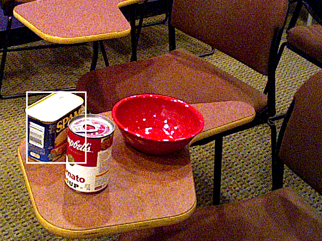
Full model
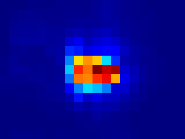
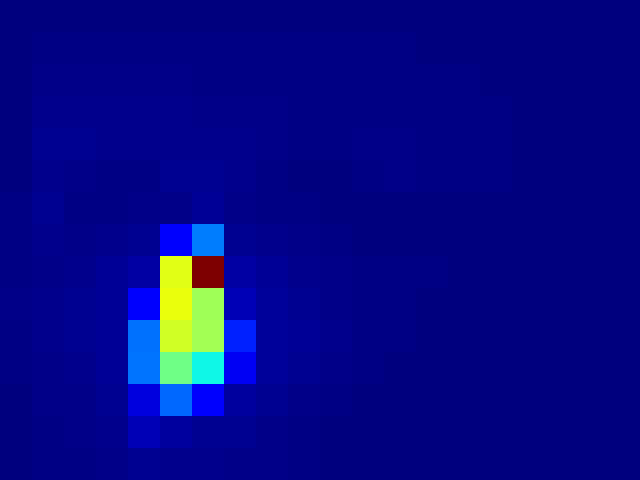
Frozen

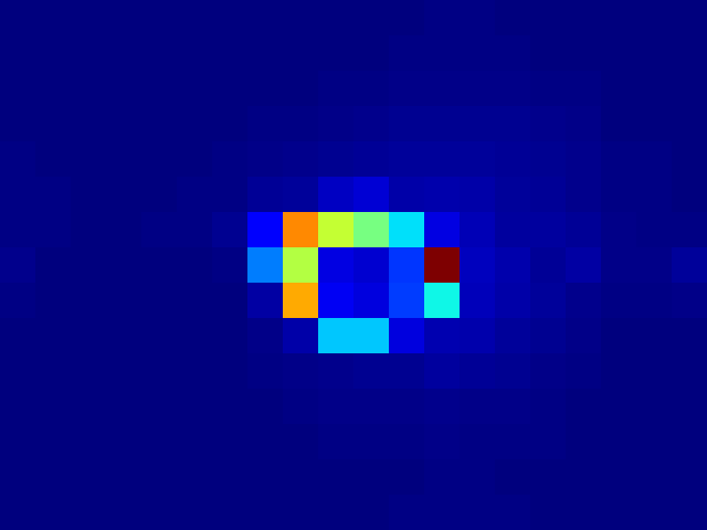
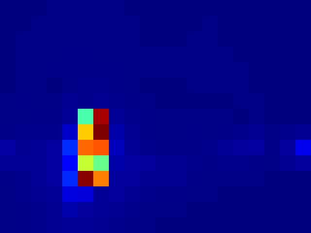
Figure 3: Object predictions of a given image (first row) and decoder attention maps for the object queries (second and third rows). Training the complete model for both object detection and pose estimation tasks (second row). Training the model first on the object detection task, and then training the frozen model on the pose estimation task (third row). Attention maps are visualized using the jet color map (shown above for reference).

4.3.1 Hyperparameters

$\alpha$ and $\beta$ hyperparameters in computing $\mathcal{L}_{box}$ (Eq. 5) are set to 2 and 5, respectively. The $\lambda_{pose}$ hyperparameter in computing $\mathcal{L}_{Hungarian}$ (Eq. 4) is set to 0.05, and the cardinality of the predicted set $N$ is set to 20. The model takes the image of the size 640 $\times$ 480 as input and is trained using the AdamW optimizer [17] with an initial learning rate of $10^{-4}$ and for 78K iterations. The learning rate is decayed to $10^{-5}$ after 70K iterations, and the batch size is 32. Moreover, gradient clipping with a maximal gradient norm of 0.1 is applied. In addition to YCB-V dataset images, we use the synthetic dataset provided by PoseCNN for training our model.

4.4 Results

In Table 1, we present the per object quantitative results of T6D-Direct on the YCB-V dataset. We compare our results with PoseCNN [35], PVNet [20] and DeepIM [14]. In terms of the approach, T6D-Direct is comparable to PoseCNN; both are direct regression methods, whereas PVNet is an indirect method, and DeepIM is a refinement-based approach. In terms of both the AUC of ADDS and AUC of ADD(-S) metrics, T6D-Direct outperforms PoseCNN and outperforms the AUC of ADD(-S) results of PVNet. For a fair comparison, we follow the same object symmetry definition and evaluation procedure described by the YCB-Video dataset [35].

Some qualitative results are shown in Fig. 5. To demonstrate the ability of the Transformer architecture to model dependencies between pixels over the whole image instead of a just small local neighborhood, in Fig. 4, we visualize the self-attention maps for three pixels belonging to three objects in the image. All three pixels lie on the same horizontal line but attend to different parts of the image.

Table 1: Pose prediction results on the YCB-V Dataset. The symmetric objects are denoted by *.

Metric	AUC of ADD-S			AUC of ADD(-S)
Object	PoseCNN	T6D-Direct	DeepIM	PoseCNN	PVNet	T6D-Direct	DeepIM
master_chef_can	84.0	91.9	93.1	50.9	81.6	61.5	71.2
cracker_box	76.9	86.6	91.0	51.7	80.5	76.3	83.6
sugar_box	84.3	90.3	96.2	68.6	84.9	81.8	94.1
tomato_soup_can	80.9	88.9	92.4	66.0	78.2	72.0	86.1
mustard_bottle	90.2	94.7	95.1	79.9	88.3	85.7	91.5
tuna_fish_can	87.9	92.2	96.1	70.4	62.2	59.0	87.7
pudding_box	79.0	85.1	90.7	62.9	85.2	72.7	82.7
gelatin_box	87.1	86.9	94.3	75.2	88.7	74.4	91.9
potted_meat_can	78.5	83.5	86.4	59.6	65.1	67.8	76.2
banana	85.9	93.8	72.3	91.3	51.8	87.4	81.2
pitcher_base	76.8	92.3	94.6	52.5	91.2	84.5	90.1
bleach_cleanser	71.9	83.0	90.3	50.5	74.8	65.0	81.2
bowl*	69.7	91.6	81.4	69.7	89.0	91.6	81.4
mug	78.0	89.8	91.3	57.7	81.5	72.1	81.4
power_drill	72.8	88.8	92.3	55.1	83.4	77.7	85.5
wood_block*	65.8	90.7	81.9	65.8	71.5	90.7	81.9
scissors	56.2	83.0	75.4	35.8	54.8	59.7	60.9
large_marker	71.4	74.9	86.2	58.0	35.8	63.9	75.6
large_clamp*	49.9	78.3	74.3	49.9	66.3	78.3	74.3
extra_large_clamp*	47.0	54.7	73.2	47.0	53.9	54.7	73.3
foam_brick*	87.8	89.9	81.9	87.8	80.6	89.9	81.9
MEAN	75.9	86.2	88.1	61.3	73.4	74.6	81.9

Figure 4: Encoder self-attention. We visualize the self-attention maps for three pixels belonging to three objects in the image. All three pixels lie on the same horizontal line but attend to different parts of the image. Attention maps are visualized using the jet color map (shown above for reference).

Ours    PoseCNN

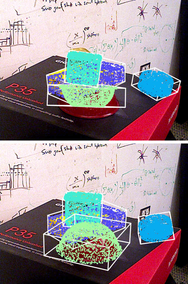
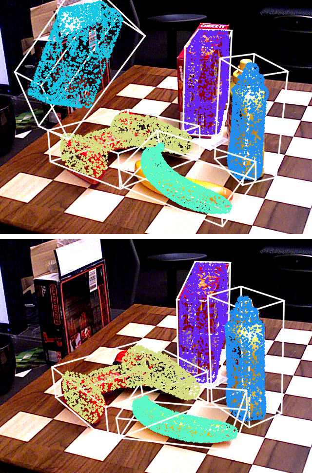
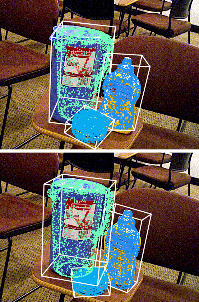
Figure 5: Qualitative examples from the YCB-V Dataset. Top row: PoseCNN [35]. Bottom row: our predictions.

4.5 Inference time analysis

Table 2: Comparison with state-of-the-art methods on YCB-V. In terms of the ADD(-S) 0.1d metric, we achieve the state-of-the-art result. ^† indicates that the method is refinement-based. Inference time is the average time taken for processing all objects in an image.

Method	ADD(-S)	AUC of ADD-S	AUC of ADD(-S)	Inference Time [$\mathrm{s}\text{/}$]
CosyPose† [13]	-	89.8	84.5	0.395
PoseCNN [35]	21.3	75.9	61.3	*$>$0.250
SegDriven [10]	39.0	-	-	*0.050
Single-Stage [9]	53.9	-	-	*0.022
GDR-Net [33]	49.1	89.1	80.2	0.065
T6D-Direct (Ours)	48.7	86.2	74.6	0.017

Since the prediction heads generate $N$ predictions in parallel, the inference of our model is not dependent on the number of objects in an image. However, having a smaller cardinality of the prediction set requires estimating fewer object queries and facilitates faster inference time. Thus, we set N to 20. On an NVIDIA 3090 GPU and Intel 3.70 GHz CPU, our model runs at 58 fps which makes our model ideal for real-time applications.

5 Ablation study

In this section, we explore the effect of various training strategies, different loss functions, and egocentric vs. allocentric rotation representations on the T6D-Direct model performance for the YCB-V dataset.

5.0.1 Effectiveness of loss functions

In Table 3, we examine the performance of our model using the symmetry aware version of Point Matching loss with $\ell_{2}$ norm [14, 35] which, in contrast to the disentangled loss presented in Section 3.1.6, couples the rotation and translation components. This loss function results in the best AUC of ADD(-S) metric. Moreover, since the symmetry aware SLoss component of the Point Matching loss is computationally expensive, we experimented with training our model using only the PLoss component. Interestingly, the ADD(-S) result of the model trained using only the PLoss component (row 5) is only slightly worse than the model trained using the both components (row 1).

Table 3: Ablation study on YCB-V. We provide results of our method with different loss functions and training schemes.

Row	Method	ADD(-S)	AUC of ADD(-S)
1	T6D-Direct with Point Matching loss	47.0	75.6
2	1 + multi-stage training	20.5	59.1
3	1 + pose matching cost component	42.8	71.7
4	1 + allocentric R6d	42.9	74.4
5	T6D-Direct with PLoss	45.8	74.4
6	T6D-Direct	48.7	74.6

5.0.2 Effectiveness of training strategies

As discussed in Section 4.3, there are two training schemes: single-stage and multi-stage. In the multi-stage scheme, we train the Transformer model for object detection and only train the FFNs for pose estimation, whereas in the single-stage scheme, we train the complete model in one stage. In our experiments, as shown in Table 3, multi-stage training (row 2) yielded inferior results, although both schemes were pretrained on the COCO dataset. This demonstrates that the Transformer model is learning the features specific to the 6D object pose estimation task on YCB-V, and COCO fine-tuning mainly helps in faster convergence during training and not in more accurate pose estimations. We thus believe that most large-scale image datasets can serve as pretraining data source. We also provide the results of including the pose component in the bipartite matching cost mentioned in Eq. 3. Including the pose component (row 3) does not provide any considerable advantage; thus, we include only the class probability and bounding box components in the bipartite matching cost in all further experiments. Further, egocentric rotation representation (row 1) performed slightly better than allocentric representation (row 4). We hypothesize that supplementing RGB images with positional encoding allows the Transformer model to learn spatial features efficiently. Therefore, the allocentric representation does not have any advantage over the egocentric representation.

6 Conclusion

We introduced T6D-Direct, a transformer-based architecture for multi-object 6D pose estimation. Equipped with multi-head attention mechanism, our model obtains competitive results in the task of direct 6D pose estimation without any dense features. Unlike the standard multi-staged methods, our formulation of multi-object 6D pose estimation as a set prediction problem allows estimating the 6D pose of all the objects in a given image in one forward pass. Furthermore, our model is real-time capable. In the future, we plan to explore the possibilities of incorporating dense estimation features into our architecture and improve the performance further.

References

- Carion et al. [2020] Carion, N., Massa, F., Synnaeve, G., Usunier, N., Kirillov, A., Zagoruyko, S.: End-to-end object detection with transformers. In: ECCV, pp. 213–229 (2020)
- Deng et al. [2009] Deng, J., Dong, W., Socher, R., Li, L.J., Li, K., Fei-Fei, L.: Imagenet: A large-scale hierarchical image database. In: CVPR, pp. 248–255 (2009)
- Dosovitskiy et al. [2021] Dosovitskiy, A., Beyer, L., Kolesnikov, A., Weissenborn, D., Zhai, X., Unterthiner, T., Dehghani, M., Minderer, M., Heigold, G., Gelly, S., Uszkoreit, J., Houlsby, N.: An image is worth 16x16 words: Transformers for image recognition at scale. In: ICLR (2021)
- Girshick [2015] Girshick, R.: Fast r-cnn. In: ICCV, pp. 1440–1448 (2015)
- He et al. [2016] He, K., Zhang, X., Ren, S., Sun, J.: Deep residual learning for image recognition. In: CVPR, pp. 770–778 (2016)
- Hinterstoisser et al. [2013] Hinterstoisser, S., Lepetit, V., Ilic, S., Holzer, S., Bradski, G., Konolige, K., Navab, N.: Model based training, detection and pose estimation of texture-less 3D objects in heavily cluttered scenes. In: ACCV, pp. 548–562, Berlin, Heidelberg (2013)
- Hodaň et al. [2020] Hodaň, T., Sundermeyer, M., Drost, B., Labbé, Y., Brachmann, E., Michel, F., Rother, C., Matas, J.: Bop challenge 2020 on 6d object localization. In: ECCV, pp. 577–594 (2020)
- Hosang et al. [2017] Hosang, J., Benenson, R., Schiele, B.: Learning non-maximum suppression. In: CVPR, pp. 4507–4515 (2017)
- Hu et al. [2020] Hu, Y., Fua, P., Wang, W., Salzmann, M.: Single-stage 6d object pose estimation. In: CVPR (2020)
- Hu et al. [2019] Hu, Y., Hugonot, J., Fua, P., Salzmann, M.: Segmentation-driven 6D object pose estimation. In: CVPR, pp. 3385–3394 (2019)
- Kehl et al. [2017] Kehl, W., Manhardt, F., Tombari, F., Ilic, S., Navab, N.: SSD-6D: Making RGB-based 3D detection and 6D pose estimation great again. In: CVPR, pp. 1521–1529 (2017)
- Khan et al. [2021] Khan, S., Naseer, M., Hayat, M., Zamir, S.W., Khan, F.S., Shah, M.: Transformers in vision: A survey. arXiv:2101.01169 (2021)
- Labbe et al. [2020] Labbe, Y., Carpentier, J., Aubry, M., Sivic, J.: CosyPose: Consistent multi-view multi-object 6D pose estimation. In: ECCV (2020)
- Li et al. [2018] Li, Y., Wang, G., Ji, X., Xiang, Y., Fox, D.: DeepIM: Deep iterative matching for 6D pose estimation. In: ECCV, pp. 683–698 (2018)
- Li et al. [2019] Li, Z., Wang, G., Ji, X.: Cdpn: Coordinates-based disentangled pose network for real-time rgb-based 6-dof object pose estimation. In: ICCV (2019)
- Lin et al. [2014] Lin, T.Y., Maire, M., Belongie, S., Hays, J., Perona, P., Ramanan, D., Dollár, P., Zitnick, C.L.: Microsoft COCO: Common objects in context. In: ECCV, pp. 740–755 (2014)
- Loshchilov and Hutter [2017] Loshchilov, I., Hutter, F.: Decoupled weight decay regularization. In: ICLR (2017)
- Manhardt et al. [2018] Manhardt, F., Kehl, W., Navab, N., Tombari, F.: Deep model-based 6D pose refinement in RGB. In: ECCV, pp. 800–815 (2018)
- Oberweger et al. [2018] Oberweger, M., Rad, M., Lepetit, V.: Making deep heatmaps robust to partial occlusions for 3D object pose estimation. In: ECCV (2018)
- Peng et al. [2019] Peng, S., Liu, Y., Huang, Q., Zhou, X., Bao, H.: PVNet: Pixel-wise voting network for 6DOF pose estimation. In: CVPR, pp. 4561–4570 (2019)
- Periyasamy et al. [2018] Periyasamy, A.S., Schwarz, M., Behnke, S.: Robust 6D object pose estimation in cluttered scenes using semantic segmentation and pose regression networks. In: IROS (2018)
- Periyasamy et al. [2019] Periyasamy, A.S., Schwarz, M., Behnke, S.: Refining 6D object pose predictions using abstract render-and-compare. In: Humanoids, pp. 739–746 (2019)
- Rad and Lepetit [2017] Rad, M., Lepetit, V.: BB8: A scalable, accurate, robust to partial occlusion method for predicting the 3D poses of challenging objects without using depth. In: ICCV, pp. 3828–3836 (2017)
- Ren et al. [2015] Ren, S., He, K., Girshick, R., Sun, J.: Faster r-cnn: Towards real-time object detection with region proposal networks. In: NeurIPS, vol. 28 (2015)
- Rezatofighi et al. [2019] Rezatofighi, H., Tsoi, N., Gwak, J., Sadeghian, A., Reid, I., Savarese, S.: Generalized intersection over union: A metric and a loss for bounding box regression. In: CVPR, pp. 658–666 (2019)
- Schwarz et al. [2018] Schwarz, M., Lenz, C., García, G.M., Koo, S., Periyasamy, A.S., Schreiber, M., Behnke, S.: Fast object learning and dual-arm coordination for cluttered stowing, picking, and packing. In: ICRA, pp. 3347–3354 (2018)
- Shao et al. [2020] Shao, J., Jiang, Y., Wang, G., Li, Z., Ji, X.: PFRL: Pose-Free reinforcement learning for 6D pose estimation. In: CVPR (2020)
- Sundermeyer et al. [2018] Sundermeyer, M., Marton, Z.C., Durner, M., Brucker, M., Triebel, R.: Implicit 3D orientation learning for 6D object detection from RGB images. In: ECCV (2018)
- Tekin et al. [2018] Tekin, B., Sinha, S.N., Fua, P.: Real-time seamless single shot 6D object pose prediction. In: CVPR (2018)
- Touvron et al. [2021] Touvron, H., Cord, M., Douze, M., Massa, F., Sablayrolles, A., Jégou, H.: Training data-efficient image transformers & distillation through attention. In: ICML, pp. 10347–10357 (2021)
- Vaswani et al. [2017] Vaswani, A., Shazeer, N., Parmar, N., Uszkoreit, J., Jones, L., Gomez, A.N., Kaiser, L.u., Polosukhin, I.: Attention is all you need. In: NeurIPS, vol. 30 (2017)
- Wang et al. [2020a] Wang, G., Manhardt, F., Shao, J., Ji, X., Navab, N., Tombari, F.: Self6D: self-supervised monocular 6D object pose estimation. In: ECCV, pp. 108–125 (2020a)
- Wang et al. [2021] Wang, G., Manhardt, F., Tombari, F., Ji, X.: GDR-Net: Geometry-guided direct regression network for monocular 6D object pose estimation. In: CVPR (2021)
- Wang et al. [2020b] Wang, H., Zhu, Y., Green, B., Adam, H., Yuille, A., Chen, L.C.: Axial-DeepLab: stand-alone axial-attention for panoptic segmentation. In: ECCV, pp. 108–126 (2020b)
- Xiang et al. [2018] Xiang, Y., Schmidt, T., Narayanan, V., Fox, D.: Posecnn: A convolutional neural network for 6d object pose estimation in cluttered scenes. RSS (2018)
- Zhou et al. [2019] Zhou, Y., Barnes, C., Lu, J., Yang, J., Li, H.: On the continuity of rotation representations in neural networks. In: CVPR, pp. 5745–5753 (2019)
- Zhu et al. [2021] Zhu, X., Su, W., Lu, L., Li, B., Wang, X., Dai, J.: Deformable detr: Deformable transformers for end-to-end object detection. In: ICLR (2021)