Marginals Versus Copulas: Which Account For More Model Risk In Multivariate Risk Forecasting?

ABSTRACT

Copulas. We study the model risk of multivariate risk models in a comprehensive empirical study on Copula-GARCH models used for forecasting Value-at-Risk and Expected Shortfall. To determine whether model risk inherent in the forecasting of portfolio risk is caused by the candidate marginal or copula models, we analyze different groups of models in which we fix either the marginals, the copula, or neither. Model risk is economically significant, is especially high during periods of crisis, and is almost completely due to the choice of the copula. We then propose the use of the model confidence set procedure to narrow down the set of available models and reduce model risk for Copula-GARCH risk models. Our proposed approach leads to a significant improvement in the mean absolute deviation of one day ahead forecasts by our various candidate risk models.

Keywords: OR in Banking, Risk Analysis, Finance, Copula, Model Risk.

JEL Classification Numbers: G17, G32, C53, C58.

1 Introduction

Financial institutions employ quantitative models in almost all aspects of their risk management (e.g., for the pricing of derivatives, the modeling of credit risk portfolios, or the forecasting of market risk measures). The increase in the multiplicity and the complexity of these risk models is driven by both the occurrence of tail risks after the Great Financial Crisis as well as the incentives set by the Basel II/III and Solvency II regulations for institutions to develop and use internal quantitative models. However, any risk measurement that does not rely on a standard approach prescribed by regulators will require the risk manager to select a candidate risk model thus introducing potential model risk. In this paper, we study such model risk for a class of prominent models for multivariate risk forecasting: Copula-GARCH models. As our main result, we find that copulas account for considerably more model risk than marginals in multivariate models.

We study the model risk of multivariate risk models in a comprehensive empirical study using Copula-GARCH models. Our ultimate goals are to quantify model risk in multivariate forecasts of portfolio Value-at-Risk (VaR) and Expected Shortfall (ES), and to propose ways how to reduce model uncertainty. To achieve these goals, we forecast the VaR and ES for a large number of multivariate portfolios using a variety of Copula-GARCH models. The first question which we want to answer is whether the model risk inherent in the forecasting of portfolio risk is caused by the candidate marginal or copula models. For this, we analyze different groups of models in which we fix either the marginals, the copula, or neither. We then propose the use of the model confidence set procedure proposed by Hansen et al. (2011) to narrow down the set of available models and reduce model risk for Copula-GARCH risk models.

As our first main result, we find that model risk is economically significant for the set of candidate multivariate models that we consider. For a portfolio with a value of $100,000 and a holding period of 10 days, model risk can account for an absolute deviation in VaR (ES) of up to $2,678 ($2,264). Interestingly, these high levels of model risk are almost completely due to the choice of the copula with the choice of marginal model having only a small effect on overall model uncertainty. Finally, and not surprisingly, periods of high market volatility lead to a surge in model risk. We then propose the use of the model confidence set procedure to narrow down the set of available models and reduce model risk for Copula-GARCH risk models. Our proposed approach leads to a significant improvement in the mean absolute deviation of one day ahead forecasts by our various candidate risk models.

Our paper paper contributes to several strands in the literature on both model risk and multivariate risk forecasting. First, our paper complements several studies on the importance of moral risk in financial risk forecasting. In this field, early studies focused on the choice of models for pricing option contract. For example, Green and Figlewski (1999) and later Hull and Suo (2002) show that model risk in the form of inaccurate volatility forecasts and modeling errors in the implied volatility function can lead to significant risk exposure for option writers. In a similar setting, Cont (2006) proposes a simple framework for quantifying model uncertainty in derivatives pricing. While our paper relies on similar definitions of model risk, we do no restrict our study to derivatives pricing but instead focus on the more general problem of studying model risk in the context of market risk forecasting. After the Great Financial Crisis, interest in the study of model risk surged again as the failure of market and credit risk models to adequately capture tail risks was seen as a major driver of the global crisis. In this strand of the literature, Alexander and Sarabia (2012) and Glasserman and Xu (2014) both propose new methodologies for quantifying model risk with the former concentrating on Value-at-Risk models and the latter studying credit and counterparty risk. Similarly, Danielsson et al. (2016) study model risk of models used for forecasting systemic risk. In contrast to these related studies, we focus on multivariate risk models and disentangle the parts of model risk that are due to the separate modeling of the marginal behavior and the dependence structure in copula models.

Moreover, our study is also related to a large strand of literature on copula modeling in quantitative risk management. In this field of research, the majority of studies have been concerned with the model risk caused by the need of selecting the best parametric copula family in a multivariate risk model (see, e.g., Kole et al., 2007; Savu and Trede, 2008; Genest et al., 2009; Dißmann et al., 2013). In addition, several recent papers propose new copula models that are suitable for modeling dependence structures in high-dimensional financial data (e.g., large market risk portfolios) (see, e.g., Aas et al., 2009; Brechmann and Czado, 2013; Oh and Patton, 2017, 2018; Bassetti et al., 2018). Finally, several papers have looked at the superiority of copula models over competing one-dimensional or correlation-based risk models (see, e.g., Jondeau and Rockinger, 2006; Grundke and Polle, 2012; Weiß, 2013). Complementing these studies, our paper analyzes the economic significance and the source of model risk in copula risk models. As such, it is the first to quantify the extent to which model risk stemming from the choice of a parametric copula can lead to significant additional risk exposure for risk managers and investors.

The rest of the paper is structured as follows. In Section 2, we present the models and backtests employed in our empirical study as well as a description of the Model Confidence Set. In Section 3, we shortly discuss the financial market data used in our study. Sections 4 and 5 present our main results of the analysis of model risk and the proposed use of the Model Confidence set, respectively. Section 7 concludes.

2 Market risk models and model risk

This section provides details on the estimation of market risk via copula GARCH models, backtesting of the risk estimates as well as the calculation of model risk. In addition, we introduce the model confidence set (MCS) procedure due to Hansen et al. (2011) yielding a set of models that contains the best model with a certain probability.

2.1 Multivariate estimation of market risk

As a consequence of the theorem by Sklar (1959), one can separate the modeling of the marginals and the dependence of multivariate return series. This is usually done by using GARCH-type models to filter the univariate time series while copulas are subsequently applied to model the dependence structure between different assets in a given portfolio. We will now present the corresponding two step approach to multivariate time series modeling in more detail.

We start with modeling the marginals as ARMA-GARCH-type processes with various error distributions. We consider not only the standard GARCH model by Bollerslev (1986), but also employ the EGARCH model by Nelson (1991), GJR-GARCH model by Glosten et al. (1993), T-GARCH model by Zakoian (1994), and aPARCH model by Ding et al. (1993). These models are all nested within the fGARCH model by Hentschel (1995). We provide the specifications for an ARMA(p,q)-GARCH(r,s) process in Section IA.1.1 in more detail as this is a very popular representative of this class of models. For the remaining models we refer to the reference guide by Bollerslev (2010) as well as to the original papers.

We consider innovations following a normal distribution, a Student-t distribution, a skewed Student-t distribution, and a generalized error distribution. Apart from the normal distribution, these distributions are able to account for skewness and/or fat tails in the data. Combining these four distributions with the five GARCH-type models yields in total 20 different (univariate) specifications that we use to fit ARMA(1,1)-GARCH(1,1)-type processes to the return series.

In a second step, we apply copula dependence models to the GARCH filtered data from the first step. Copulas are multivariate distributions with all marginals being uniformly distributed in the interval $[0,1]$. For a $d$-dimensional distribution with distribution function $F$ and marginals $F_{1},\dots,F_{d}$, the copula associated with $F$ is a function $C:[0,1]^{d}\to[0,1]$ satisfying

$$F(\mathbf{x})=C\big{(}F_{1}(x_{1}),\dots,F_{d}(x_{d})\big{)}$$

for $x=(x_{1},\dots,x_{d})\in\mathbb{R}^{d}.$ On the basis of the two step approach lies the fact that copulas enable us to model the dependence structure of multivariate distributions separately from the marginal distributions. This is a consequence of the theorem by Sklar (1959), see Section IA.1.2 for more details.

We consider various copula functions. We include the Gaussian and Student-t copulas because they are widely used in financial applications (cf. Cherubini et al., 2004; McNeil et al., 2005). We additionally employ the Archimedean copulas Clayton, Gumbel, Frank, and Joe copula. This gives us further possibilities to model multivariate dependence as for example the Clayton copula allows for modeling a positive lower tail dependence. For more details on copulas in general and the copulas used in this paper we refer to the comprehensive books by by Joe (2001) and Nelsen (2006).

While the Gaussian and Student-t copulas can only model symmetric dependencies using correlation matrices, Archimedean copulas typically have only one (like the above mentioned copulas) or two parameters, which is very restrictive. So-called pair copula constructions (also referred to as vine copulas) offer a very convenient possibility for a highly flexible modeling of the dependence structure. Originally introduced by Joe (1996), further significant contributions have been made by Bedford and Cooke (2001, 2002), and Kurowicka and Cooke (2006). Additionally, we include the Gaussian mixture copula due to Tewari et al. (2011) that can capture multi-modal dependencies as well as asymmetric and tail dependencies. Another very popular model is the Dynamic Conditional Correlation (DCC) model due to Engle and Sheppard (2001) and Engle (2002). Though not a copula model, the DCC model fits perfectly into our framework. It allows for a two stage estimation of the model parameters where in a first stage GARCH-type models are fitted to each of the univariate return series. The conditional correlation matrix is derived in a second step to model the multivariate dependence between the return series. In the following, we will therefore subsume all models under the term copula GARCH models.

For each combination of the considered copula and ARMA-GARCH-type models we now proceed as follows to obtain one day ahead VaR and ES forecasts for a given portfolio of $K$ assets: First, we simulate 10,000 $K$-dimensional vectors of standardized residuals from the fitted copula. Based on the parameters and ex-ante mean and variance forecasts from the ARMA and GARCH-type models that have already been fitted to the univariate return series, we transform the simulated standardized residuals into 10,000 return forecasts for each of the portfolio constituents. We finally derive 10,000 portfolio returns and calculate the VaR as the sample quantile and the ES as the conditional mean of the returns falling below this quantile (both values are subsequently multiplied by $(-1)$). This procedure is repeated on a daily basis based on a moving window of data. For more details we refer to Brechmann and Czado (2013), see also Aas and Berg (2009), Ausin and Lopes (2010), and Nikoloulopoulos et al. (2012). One important advantage of this approach is that copulas and marginals only have to be fitted once to consider various portfolio weights. This is because the weights enter into the procedure only at the end when calculating the portfolio returns.

2.2 Backtests

Our aim is to analyze the risk associated with choosing an appropriate model from a variety of valid candidate models, not to identify the optimal model for forecasting VaR and ES estimates. Nonetheless, we backtest our risk forecasts before measuring the model risk itself for the following reasons: First, in order to determine a set of valid candidate models, we need to prevent our results from being biased by erroneous risk forecasts due to misspecified models. Second, the approach of calculating model risk after having applied backtests is also favorable from a more practical perspective. The Basel III regulation requires banks to backtest their (internal) market risk models. For banks, uncertainty on the model choice is, essentially, uncertainty on the choice of models that have not been rejected by backtests. This is in line with our calculation of model risk.

We measure the quality of the VaR estimates using the duration-based test of Christoffersen (2004). The test follows a more general approach of independence rather than focussing on the independence of VaR violations only. The test assumes that in the case of independent VaR violations, the time between violations must be independent of the time to a previous violation. In simple terms, this means that the probability that a VaR violation will occur in the next 10 days must be independent of whether the last one occurred in the last 10 or 100 days. Christoffersen (2004) shows that his duration-based test tends to reveal VaR methods that violate the independence property in realistic situations more often and hence has better power properties than former tests. For more details on the duration-based test we refer to IA.1.3 as well as to the original paper.

Since the VaR has been replaced by the ES as the leading market risk measure in regulatory requirements, the debate on suitable backtesting for the ES has also been increasing in the literature. In view of the regulatory requirements and because the VaR does not have to be issued by financial institutions, ideally a backtest should only determine the quality of the ES model based on real data and the forecasts. In practice, however, many backtests require additional input variables or assumptions. We evaluate ES estimates using a comparatively new test by Nolde and Ziegel (2017), which is based on the concept of conditional calibration (CC). For a brief description of the test, we refer to IA.1.4 and the original paper. The CC test requires in its simple version both VaR and ES forecasts. We find the use of a joint backtest of VaR and ES predictions sensible for the following reasons: First, in line with Bayer and Dimitriadis (2020b), we find that the ES is by definition closely related to the VaR and thus suitable ES forecasts are based on adequate VaR estimations. Secondly, we apply the MCS procedure at a later point of our analysis. This method is again based on functions that require both VaR and ES forecasts. Consequently, the use of a joint VaR and ES backtest is appropriate.

By using a joint backtest for the ES, it should be noted that this is a possible reason why more models fail the backtest than in the case of the VaR. For this reason and because different confidence levels are considered in the baseline case, we separate the analysis of the VaR and the ES in terms of model risk.

2.3 Model risk

Financial risk cannot be measured directly, but only be estimated using statistical models. However, it is well known that distinct models may differ vastly in their risk predictions (see, e.g., Danielsson et al., 2016). In the literature one can find various approaches towards defining and measuring model risk. A large part of research focuses on the factors that control model risk within models such as the misspecification of the underlying theoretical models (Green and Figlewski, 1999) or assumptions made about unknown (or unobservable) parameters, distributions, or other model specifications (e.g., Hull and Suo, 2002; Alexander and Sarabia, 2012; Glasserman and Xu, 2014; Boucher et al., 2014). However, we focus on a more general problem: With a variety of standard VaR and ES models within the industry, uncertainty about the choice of a particular model creates model risk per se. Especially, our aim is not to identify an optimal model for forecasting the VaR or ES, but to analyze the risk that emerges from the presence of a large set of valid candidate models. Our notion of model risk as uncertainty on the model choice itself in the presence of many possible alternative models is most closely related to Cont (2006) and Danielsson et al. (2016).

We consider all VaR and ES models that are not rejected in the respective backtest as viable candidates for measuring market risk. This leaves us with a large number of models and corresponding risk forecasts for the same quantity. As a measure of model risk, we quantify the level of disagreement between the individual estimates based on the mean absolute deviation (mad), the standard deviation (sd), and the interquartile range (iqr). The mean absolute and the standard deviation are intuitive and plausible measures since both take into account how much the models deviate from the average forecast. The iqr of an observation variable is the difference of its 75% and 25% percentiles and consequently a measure of the maximum disagreement within the 50% of observations around the median. We choose the mad as our main measure of model risk for the following reasons: First, the mad is more robust against outliers than the sd. Second, it can easily be interpreted in absolute terms relative to a given portfolio value and reflects the deviation of a forecast by a randomly chosen model from the average risk forecast. Finally, since our main analysis relies on forming different groups of models, we need a measure of model risk that is as independent as possible from the number of models within a particular group. For these reasons, we focus on the mad to measure model risk and include the measures sd and iqr for robustness.

2.4 Model confidence set

Researchers, practitioners, and regulators are often confronted with situations where a variety of models for computing a specific estimate, e.g., for VaR or ES forecasts, exist. Optimally, one would like to know which of the many available models is the best. However, in many situations this question cannot be answered, especially when the set of competing methods is large and the data are not sufficiently informative. Yet, one can try to reduce the set of available models to a smaller set of alternatives. This can be done by the model confidence set (MCS) procedure by Hansen et al. (2011).

The MCS procedure yields a set of models (the model confidence set) that contains the best model with a certain probability. That is, the procedure does in general not identify a best model nor does it assume that a particular model represents the true data generating process. Instead, the MCS can be seen as an analogue to a confidence interval that contains a parameter of interest with a specified probability. An important advantage of the MCS procedure over methods that choose a single model is that it accounts for the informativeness of the data at hand. When data are very informative one may obtain a MCS that consists of only the best model. Less informative data, on the other hand, may lead to a MCS containing several models as the data make it hard to distinguish between models. Additionally, the MCS procedure allows for valid statements about significance that are not hampered by multiple pairwise comparisons (Hansen et al., 2011). These attractive features make it interesting to apply the MCS procedure to our set of VaR and ES models. The MCS procedure might help in further narrowing down the set of valid candidate models (after applying the backtests) such that the remaining models exhibit a lower model risk.

The construction of the MCS procedure relies on an equivalence test, $\delta_{\mathcal{M}}$, and an elimination rule, $e_{\mathcal{M}}$. First, the equivalence test is applied to the set of candidate models $\mathcal{M}^{0}$. If equivalence is rejected at a given confidence level $\alpha$, this implies that the candidate models are not equally “good”. Thus, the elimination rule is applied to remove a poorly performing model from the set $\mathcal{M}^{0}$. These two steps are repeated until the equivalence test is not rejected for the first time. The remaining elements of $\mathcal{M}^{0}$ are then considered as the model confidence set $\hat{\mathcal{M}}_{1-\alpha}$. As the same confidence level $\alpha$ is used in each iteration for the equivalence test, the procedure guarantees that $\lim_{n\to\infty}P(\mathcal{M}^{*}\subseteq\hat{\mathcal{M}}^{*}_{1-\alpha})\geq 1-\alpha$, where $\mathcal{M}^{*}$ denotes the true set of best models and $n$ is the number of observations per model. Additionally, the MCS procedure provides p-values for each model that can be interpreted as the probability that the respective model is among the best alternatives in $\mathcal{M}^{0}$. For more details on the procedure we refer to Section IA.1.5 and to the original paper.

In the MCS approach, models are evaluated based on a user-defined loss function. For evaluating the forecast accuracy of risk models it is natural to compare the forecasts to the realized financial losses over a period of time. Nolde and Ziegel (2017) highlight that for comparing different models’ risk forecasts elicitability of the risk measure is a desirable property. Generally speaking, a risk measure is elicitable if it minimizes the expected value of a scoring function. Elicitability is a property that has been proven to be useful for forecast ranking, comparative backtesting, and for model selection (Nolde and Ziegel, 2017).

As the VaR represents a quantile of a probability distribution (multiplied by -1) it is well known to be elicitable (see, e.g., Koenker and Bassett, 1978). The associated scoring function, the so-called check-function, is given by

$$L_{VaR}(r_{t},VaR_{\alpha}^{t},\alpha):=\big{(}r_{t}-(-VaR_{\alpha}^{t})\big{)}\cdot\big{(}\alpha-\mathbb{I}_{(-\infty,0)}(r_{t}-(-VaR_{\alpha}^{t}))\big{)},$$

where $r_{t}$ and $VaR_{\alpha}^{t}$ denote the realized return and the VaR forecast with coverage level $\alpha$ (and confidence level $1-\alpha$) at day $t$ and $\mathbb{I}_{(-\infty,0)}$ denotes the characteristic function of the open interval $(-\infty,0)$. We choose this scoring function as the loss function for the VaR in the MCS framework.

As opposed to the VaR, the ES alone is not elicitable. Instead, Fissler and Ziegel (2016) show that ES and VaR are jointly elicitable, see also Acerbi and Székely (2014). There is a growing body of literature building on this result, see, e.g., Fissler et al. (2016); Nolde and Ziegel (2017) for forecast comparisons and Patton et al. (2019); Barendse et al. (2019); Bayer and Dimitriadis (2020b) for applications in a regression procedure. As the ES is only jointly elicitable with the VaR, we choose a loss function for the ES that is based on both VaR and ES forecasts as input into the MCS procedure. This is consistent with the conditional calibration backtest introduced in Section 2.2 that is used to determine the set of candidate models for the ES. As Nolde and Ziegel (2017) provide a joint scoring function for the VaR and the ES only in a general form, we adopt the 0-homogeneous version introduced in Patton et al. (2019)

$$L_{ES}(VaR_{\alpha}^{t},ES_{\alpha}^{t},r_{t},\alpha):=\frac{1}{\alpha ES_{\alpha}^{t}}\cdot\mathbb{I}_{(-\infty,0)}(r_{t}+VaR_{\alpha}^{t})\cdot(-VaR_{\alpha}^{t}-r_{t})+\frac{VaR_{\alpha}^{t}}{ES_{\alpha}^{t}}+\log(ES_{\alpha}^{t})-1,$$

where the notation is as above. For an implementation of the MCS procedure we rely on the R-package MCS by Catania and Bernardi (2017). For more details we refer to Section 5.

3 Data

We form well diversified portfolios consisting of equity indices (developed and emerging markets), bond indices (governement, corporate, and high-yield bonds) as well as commodity and real estate indices. Therefore, we retrieve the total return indices (in US$) of the following set of indices from Datastream: Stoxx Europe 600, Dow Jones Industrial Average, FTSE Developed Asia Pacific Index, MSCI Emerging Markets Index, S&P U.S. Treasury Bond Index, S&P 500 Investment Grade Corporate Bond Index, S&P U.S. High Yield Corporate Bond Index, S&P Pan-Europe Developed Sovereign Bond Index, S&P GSCI, and Developed Markets Datastream Real Estate Index. The sample period is January 2001 to December 2018. Next, we calculate geometric returns that allow us to easily derive portfolio returns. For our main analysis we focus on an equally weighted portfolio. This corresponds to a portfolio consisting of 40% stocks, 40% bonds, 10% commodities, and 10% real estate. For robustness we also consider portfolios based on random portfolio weights that were drawn from a unit-simplex. Summary statistics on the equally weighted portfolio returns as well as on the individual index returns can be found in Table I.

– Insert Table I about here. –

We calculate daily VaR and ES estimates based on 180 different model specifications of copula GARCH models, see Section 2.1 for details. Additionally, we derive risk estimates from univariate GARCH-type models applied to the portfolio return series. Estimations are performed based on various confidence levels (99.9%, 99%, 97.5%, and 95%) using a moving window of 500 days corresponding to approximately two years of daily observationsand a forecast horizon of one day. We clean the risk estimates from outliers that are due to convergence errors in fitting the copula GARCH models.

Subsequently, we perform VaR or ES backtests to determine the set of candidate models that enter into the calculation of model risk on a daily basis. The backtests are based on a confidence level of 99% in line with Basel Committee on Banking Supervision (2019) and a moving window of 500 days. Note that by employing a moving window for the backtests, we avoid introducing a look-ahead bias into the selection of the set of candidate models. In our main analysis, we rely on the duration-based VaR backtest by Christoffersen (2004) and the conditional calibration ES backtest by Nolde and Ziegel (2017), see Section 2.2 for details.

Afterwards, we calculate model risk on a daily basis for the risk models that have passed the respective backtest. Note that by using moving windows the composition of the set of candidate models varies over time. Since VaR and ES estimations as well as backtests are performed based on a 500 day moving window in our baseline analysis, we obtain daily model risk estimates from day 1001 onwards. This corresponds to the time period from November 4, 2004 until December 31, 2018. We obtain model risk estimates for both VaR and ES forecasts for various confidence levels and portfolio weights. In our main analysis we focus on the model risk of risk forecasts for an equally weighted portfolio and the 99% VaR and 97.5% ES in line with the Basel II and Basel III market risk regulations. Our main measure of model risk is the mean absolute deviation (mad) of risk forecasts.

4 Analysis of model risk

4.1 All multivariate models

We start with an analysis of the model risk over time and different market conditions of all multivariate VaR and ES models that passed the respective backtest. Figure 1 presents the daily model risk associated with one day ahead forecasts of the 99% VaR and the 97.5% ES in terms of mad between November 4, 2004 and December 31, 2018. The figure reveals that model risk is normally quite moderate but increases significantly during and after the global financial crisis. Summary statistics are provided in Table II. Over the entire time period, model risk is on average about 0.165% of the portfolio value for VaR forecasts and about 0.092% of the portfolio value for ES forecasts. Model risk is quite volatile over time ranging from 0.075% to 0.847% for the VaR and from 0.029% to 0.716% for the ES with a standard deviation of daily model risk estimates of more than half of the average model risk.

– Insert Figure 1 and Table II about here. –

Model risk is especially pronounced during times of financial turmoil. During the years 2008-2009 (in the following referred to as the crisis period) the average model risk is 0.286% of the portfolio value for the VaR and 0.145% for the ES. That is, the average model risk more than doubles compared to the period before 2008 (the pre-crisis period) with an average VaR of 0.119% and ES of 0.063 %. The maximum model risk values are realized in Q4 2008 in the follow-up of the Lehman Brothers bankruptcy on the peak of the financial crisis. The extraordinary impact of the financial crisis on model risk is further highlighted by the fact that nearly all VaR model risk values above the 99% quantile occurred in Q4 2008. The same is true for the majority of the ES model risk values.

These results can only partly be explained by an increase in volatility. On the one hand we calculate VaR and ES forecasts based on conditional volatility estimates derived from GARCH-type models. Consequently, whenever volatility is high, VaR and ES forecasts will on average also show increased levels resulting in a higher model risk. On the other hand, the average model risk in 2008-2009 is 140% higher than in the pre-crisis period for the VaR while the average level of VaR estimates is only 113% higher. Similarly, the model risk for the ES in 2008-2009 is increased by 130% while the average level of ES estimates is 119% higher. This disproportionately high increase of model risk in periods of crisis might be due to the fact that all models treat history and shocks quite differently such that a change in statistical regimes can be expected to lead to higher disagreements between risk forecasts (Danielsson et al., 2016). Following the great financial crisis, model risk does not decrease to the pre-crisis level (0.119% for the VaR and 0.063% for the ES) but remains elevated at 0.155% (VaR) and 0.090% (ES). The findings are robust to considering randomly generated portfolio weights, see Table III. Summary statistics for other measures of model risk (standard deviation, interquartile range) are provided in Table IV.

– Insert Tables III and IV about here. –

Risk models are embedded within the Basel accords and play a central role in the regulatory process to determine bank capital. That is, expensive decisions such as the amount of capital held or portfolio allocations depend on the outputs of risk forecasting models as input. We highlight this point by providing model risk estimates in absolute terms in Table II. These values can be interpreted as average deviations in regulatory capital to be held according to different models (at a particular day). We calculate model risk estimates in $ by assuming a portfolio value of $100,000 and a holding period of 10 days. Therefore, we multiply the mad values (as percentage of the portfolio value) with $100,000 and $\sqrt{10}$. We thereby emphasize that differences in model risk are not only statistically but also economically significant. This is also highlighted by Figure 2 illustrating the extent of disparity of VaR models with regard to the portfolio value. The average model risk (mad) in absolute terms over the entire time period is $522 for the VaR and $291 for the ES with maximum values of $2,678 (VaR) and $2,264 (ES).

– Insert Figure 2 about here. –

Note that model risk of VaR and ES forecasts cannot directly be compared to each other. This is due to the fact that risk forecasts entering into the calculation of model risk are determined based on different backtests for the VaR and the ES. As a result, on average 174 different model specifications enter into the model risk calculation for the VaR and only 121 specifications into the model risk calculation for the ES. The effect of choosing different backtests or no backtest at all are discussed in Section 6 in more detail.

When considering several confidence levels for VaR and ES forecasts we observe that model risk for the 99.9% VaR (0.306%) is approximately twice as high as for the 99% VaR (0.165%) which again is twice as high as for the 95% VaR (0.085%). For the 99.9% ES (0.309%), 99% ES (0.142%), 97.5% ES (0.092%), and 95% ES (0.067%) the proportions are similar, see Table VIII for more details. This rise in model risk when increasing the underlying confidence level can, however, only partially be explained by an increase in the absolute level of the risk forecasts as a consequence of the higher confidence level. That is, even when relating the average model risk to the average level of risk forecasts, model risk is more pronounced for higher confidence levels. This can be seen when looking on the ratio of average model risk divided by the average level of risk forecasts which is 0.208, 0.163, 0.142 and 0.126 for the VaR and 0.201, 0.111, 0.086 and 0.075 for the ES at the 99.9%, 99%, 97.5% and 95% confidence level, respectively. These results are not surprising as they mainly reflect that the disagreements between different models in modeling the tails of the return distributions increase when considering more extreme quantiles.

4.2 Analysis of the subgroups

The VaR and ES estimates are obtained via copula GARCH models in a two step procedure. Therefore, we turn to the question if a greater portion of model risk is attributable to the statistical modeling of the univariate marginals (via GARCH-type models) or to the estimation of the multivariate dependence structure (via copulas).

Figure 32 provides the average model risk for the 99% VaR and the 97.5% ES for on an equally weighted portfolio from November 4, 2004 to December 31, 2018 for four different groups: Group 1 covers the average model risk across the sets of models in which a copula is fixed while the marginal distribution is varied. Group 1 thus measures the impact of choosing a specific GARCH-type model for the marginals. Analogously, Group 2 captures the average model risk among sets of models with fixed marginal distributions and varying copulas. Group 3 measures the average model risk of all multivariate and Group 4 of all univariate models. Table V presents the corresponding descriptive statistics.

– Insert Figure 32 and Table V about here. –

Considering the 99% VaR, average model risk for model sets with fixed copulas is 0.052% of the portfolio value. For sets with fixed marginal distributions, on the other hand, model risk increases significantly and is three times higher with an average of 0.157% of the portfolio value. Consequently, model risk is higher when choosing a copula function from a group of feasible models compared to choosing the marginal distribution. Higher model risk in the choice of a copula means that risk forecasts in groups of models with fixed marginal distributions and varying copula function differ more from each other and are thus more dissimilar than risk forecasts of groups in which the marginal distribution varies. In absolute terms, this translates into an average difference of $164 to $498 for a portfolio with $100,000 in value and a holding period of ten days. Looking at the median of the averaged sets, the model risk is 3.5 times higher with a fixed marginal distribution.

The result of significant higher model risk due to the choice of a copula function is robust when considering model risk of VaR forecasts with respect to randomly generated portfolio weights. Following Table VI, the average model risk of such model sets with varying copulas is 0.142% of the portfolio in contrast to 0.057% when using fixed copulas.

– Insert Table VI about here. –

Besides, the result is robust with respect to both the choice of a model risk measure (see Table VII and Figure 26) and the confidence level (see Table VIII and Figure 34). Figure 34 shows, in addition to the significant rise in model risk due to the choice of a copula, that increasing the confidence level from 95% to 99.9% triples the model risk, in case of model sets with fixed copula from 0.034% to 0.108% and for fixed marginal distributions from 0.078% to 0.293%.

– Insert Tables VII and VIII about here. –

As we stated before, we do not compare VaR and ES results due to risk measure specific confidence levels as well as backtests and consequently different model sets in terms of constellation and number of models see Section 6. Also for the 97.5% ES, the results show that the model risk increases significantly with the choice of a copula function. With an average of 0.068% in comparison to 0.058% of the portfolio value, the average model risk is higher with varying compared to fixed copulas see Table V. For a portfolio of $100,000, this represents $216 as opposed to $184 in risk.

Also for the ES, the result of an significant increase in model risk when choosing a copula function is robust with respect to the portfolio weighting (see Table VI), the model risk measure (see Table VII and Figure 26) and the confidence level (see Table VIII and Figure 44). Only for a confidence level of 95% the average model risk shows identical values of 0.045% of the portfolio value for fixed and varying copulas. However, when considering the median a model set with fixed marginal distributions shows a higher model risk in value (0.041%) than a model set with fixed copulas (0.033%). Again, increasing the confidence level from 95% to 99.9% results in a higher model risk. Here, the model risk triples for sets with fixed copula (from 0.045% to 0.136%), while the model risk increases sixfold for fixed marginal distributions (from 0.045% to 0.270%), see Table VIII.

We extend the abstract representation of model risk as the mean absolute deviation of various risk forecasts by illustrating the impact of model choice regarding the multivariate dependence structure as well as univariate marginals on a portfolio with value $100,000. This is illustrated in Figure 4 for the 99% VaR and model sets with fixed copulas. In this case the model risk is induced by the choice of a GARCH model and the corresponding marginal distribution. The 20th and 80th percentile of the risk estimates are subtracted from the portfolio value to represent the range of the impact of the model choice over time. The resulting model risk range per day is averaged over the different copulas. Analogously, we illustrate the impact of the choice of a copula model in Figure 5 by fixing the marginal distribution. Again, the model risk is illustrated over a range in terms of the 20th and 80th percentile of the ten-day-ahead VaR estimates at the 99% confidence level and a portfolio value of $100,000. Figure 5 shows a higher range of portfolio value over time, illustrating clearly the result that choosing a copula function generates higher model risk than choosing a GARCH-type model and a marginal distribution.

– Insert Figures 4 and 5 about here. –

5 Model risk for models in the model confidence set

The MCS procedure by Hansen et al. (2011) yields a set of models that contains the best model with a given confidence. That is, the MCS procedure does not assume a particular model to be the true or best one. Instead, it yields a set of models that can be seen as an analogue to a confidence interval for parameters, see Section 2.4 for details. As in this paper we study the model risk of risk models that are valid ex-ante and but provide differing forecasts, the MCS procedure fits perfectly into our study. We apply the MCS procedure to the set of models that passed the (daily) backtests to further narrow the set of candidate models. We then determine the model risk corresponding to the models in the MCS to analyze if model risk can be reduced by these means.

The main results are summarized in Table IX which compares model risk values before and after applying the MCS procedure in various periods of time. For the whole period, model risk before applying the MCS procedure is on average 0.165% for the VaR and 0.092% for the ES. These values are statistically significant reduced by 23% to 0.127% for the VaR and by 3% to 0.089% for the ES when considering only the models in the MCS. For both VaR and ES this approach reduces model risk not only in the whole period but also in all sub-periods (pre-crisis, crisis, and post-crisis). The reduction of model risk for ES is, however, very small with declines ranging between 2% and 5%. Opposed to this, we can achieve substantial reductions in VaR model risk (8% in the pre-crisis, 25% in the crisis, and even 27% in the post-crisis period). A graphical representation of the model risk of VaR forecasts before and after applying the MCS procedure can be found in Figure 6.

– Insert Figure 6 and Table IX about here. –

The reduction of model risk that can be achieved corresponds largely to the percentage of models that is excluded by the MCS procedure additionally to the models that have already been removed from the set of candidate models due to the backtests. On average, only 8% of ES models that have passed the respective backtest are excluded by the MCS procedure while the same is true for 21% of the VaR models. However, after applying the MCS procedure on average less ES models (62%) than VaR models (77%) are left over. This is due to the fact that only those models that have not been rejected in the respective backtest enter into the MCS procedure and a lower fraction of ES models (67%) has not been rejected (97% for the VaR). While the percentage of models excluded is relatively stable over time for ES models, it varies for VaR models. In the pre-crisis period about 11% of VaR models are excluded (additionally to the ones rejected by the backtest) while in the crisis and post-crisis period 24% and 23% are excluded, respectively. A graphical representation of the number of models before and after applying the MCS procedure can be found in Figure 7. By excluding those models that are inferior to the ones remaining in the MCS, model risk in the post-crisis period can be reduced substantially to the level of the pre-crisis period.

– Insert Figure 7 about here. –

6 Model risk and backtesting

In line with our notion of model risk as uncertainty on the model choice itself when having to choose among many possible alternative models (cf. Cont, 2006; Danielsson et al., 2016), we include many different risk forecasts into the calculation of our model risk measure. We consider various GARCH-type models for the marginals and copula functions for the dependence structure yielding 180 different multivariate model specifications. However, to prevent our results from being biased by erroneous risk forecasts due to misspecified models, we first perform backtests to determine a set of valid candidate models on a daily basis.

In our main analysis, we rely on the duration-based VaR backtest by Christoffersen (2004) and the conditional calibration ES backtest by Nolde and Ziegel (2017). Table X provides summary statistics on the number of models passing these backtests from November 4, 2004 until December 31, 2018. After having applied the backtest for the 99% VaR, there remain on average 174 models while only 121 97.5% ES models pass the ES backtest. This difference might be explained by the fact that the conditional calibration test is a joint VaR and ES backtest while the duration-based VaR backtest is not (see Section 2.2 for details). Figure 8 illustrates the number of VaR and ES models that are not rejected by the backtests over time.

– Insert Figure 8 and Table X about here. –

For robustness, we provide summary statistics on the number of models that enter into the calculation of model risk when considering alternative backtests or when using different specifications in Table XI.

– Insert Table XI about here. –

When relying on the dynamic quantile test by Engle and Manganelli (2004), on average 71 VaR models are not rejected while the same is true for 127 ES models in the exceedance residual test by McNeil and Frey (2000). Using a moving window of 1000 days instead of 500 days reduces the average number of models to 145 for the VaR and 82 for the ES while a fixed window spanning the entire sample period leads on average to 113 VaR and 17 ES models. In the following, we focus on the impact of different backtesting specifications on our model risk estimates.

6.1 All multivariate models

Summary statistics for our main measure of model risk (mad) are presented in Table XII. There, we compare the results of our main analysis to model risk estimates obtained by using no backtests or by employing alternative backtests. For robustness, we also add results when using our main backtests with a fixed estimation window and a moving window of 1000 days (instead of 500 days), respectively.

– Insert Table XII about here. –

Over the entire sample period model risk (mad) for the 99% VaR is on average 0.165% when determining the set of candidate models via the duration-based backtest. When calculating model risk based on all 180 risk forecasts (i.e., without employing a backtest), model risk for the VaR is on average slightly lower (0.156%). When instead relying on the dynamic quantile test by Engle and Manganelli (2004), average model risk is substantially lower (0.079%). Average model risk for the 97.5% ES over the entire sample period is 0.092% in our main analysis (conditional calibration backtest) and 0.163% when not using any backtest. For the exceedance residual test by McNeil and Frey (2000) average model risk (0.114%) is higher than model risk for the conditional calibration backtest, but still much lower than in the case of not using any backtest.

6.2 The subgroups

Table XIII presents summary statistics of average model risk when using alternative backtests or no backtest at all. Again, the focus is on the comparison of model sets with fixed and model sets with varying copula function. For the 99% VaR we find that the average model risk remains identical when we do not backtest. This is true for model sets with fixed (0.052%) as well as for model sets with varying (0.157%) copula function and can be explained by the fact that the duration-based backtest by Christoffersen (2004) rejects on average only about 3.3% of VaR market risk models. In contrast, the conditional calibration backtest by Nolde and Ziegel (2017) rejects on average about 33% of models forecasting ES estimates. For model sets with fixed copula function, the model risk is almost similar (deterioration of 0.003 percentage points) if no backtest is performed. On the other hand, for model sets with varying copula and consequently fixed marginal distribution, the average model risk is reduced from 0.164% to 0.068%. In addition, Figure 92 shows that our main result of increasing model risk by choosing a copula function is robust to no prior backtesting.

– Insert Figure 92 and Table XIII about here. –

For the 99% VaR using the dynamic quantile test by Engle and Manganelli (2004), the average model risk is almost not reduced for groups with fixed copula (from 0.052% to 0.051%) and more than three times reduced for groups with varying copula (from 0.157% to 0.042%). In contrast to our baseline backtest, 60.6% of the market risk models are discarded on average. When using the exceedance residual ES backtest by McNeil and Frey (2000), average model risk for sets with fixed copulas is robust to our baseline analysis (0.058%). The alternative ES backtest rejects 29.7% of market risk models on average. For the group of model sets with fixed marginal distributions, the alternative backtest leads to a slightly higher average model risk (0.077%) than our baseline (0.068%). Again, the average model risk is reduced in comparison to no prior backtest (0.164%). These results highlight that model risk depends on the choice of the backtests, some of which are able to reduce average model risk (compared in particular to using no backtest). As a consequence, employing backtests can be seen as additional means for reducing model risk. A further analysis of the choice of backtests with regard to model risk is, however, beyond the scope of this paper.

7 Conclusion

In this paper, we study the model risk inherent in Copula-GARCH models used for forecasting financial risk. More precisely, we forecast the VaR and ES for a large number of multivariate portfolios using a variety of Copula-GARCH models. We then analyze different groups of models in which we fix either the marginals, the copula, or neither in a comprehensive empirical study to identify the main source of model risk in multivariate risk forecasting. As our first main result, we find that Copula-GARCH models come with considerable model risk that is economically significant. Interestingly, and as our second main result, we find that copulas account for considerably more model risk than marginals in multivariate models with the choice of marginal model having only a small effect on overall model uncertainty. We then propose the use of the model confidence set procedure to narrow down the set of available models and reduce model risk for Copula-GARCH risk models using ready-to-use backtests for VaR and ES, respectively. Our proposed approach leads to a significant improvement in the mean absolute deviation of one day ahead forecasts by our various candidate risk models.

The findings of our analysis stress the importance of an adequate modeling of the dependence structure inherent in financial portfolios. While the choice of marginal models is not negligible, it is however of lesser importance than selecting the right parametric copula model. In this respect, our findings are reassuring as the majority of previous papers in this field have solely concentrated on copula modeling and have relied on standard GARCH(1,1)-models for the marginals. Our quantification of the degree of model risk caused by the large set of candidate parametric copula families, however, shows that multivariate models include an economically significant amount of model risk. Using the model confidence set approach seems to alleviate this danger to some degree. Finally, our findings are of high relevance for supervisors in the banking and insurance sector as we illustrate the need for carefully checking the adequacy of a multivariate copula-based risk model.

Figure 1: Daily model risk for all multivariate models

This figure shows the model risk associated with one day ahead 99% VaR and 97.5% ES forecasts for a well diversified portfolio. Model risk is measured in terms of the mean absolute deviation (mad) of one day ahead forecasts by various risk models. Values are calculated on a daily basis between November 4, 2004 until December 31, 2018 in percent of the portfolio value based on all multivariate models that passed the respective backtest, see Section 2.2 for details.

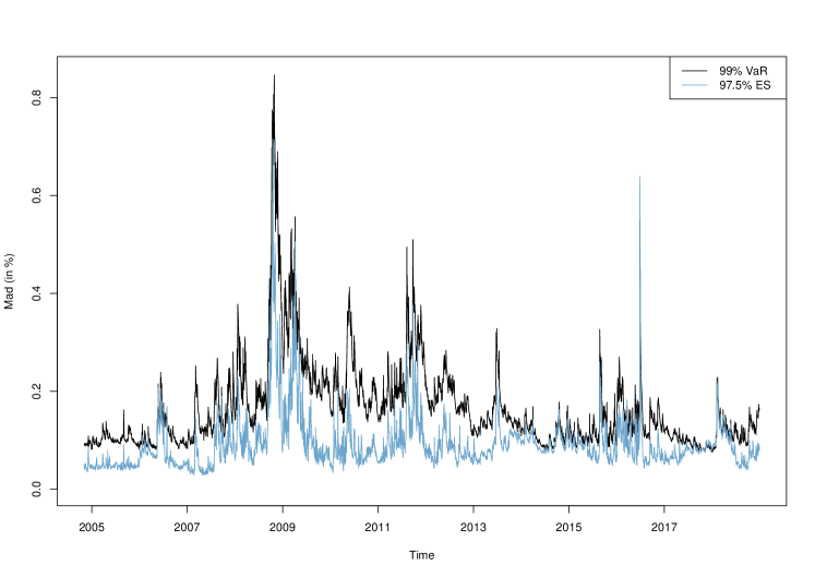
Figure 2: Potential portfolio value under financial distress

This figure illustrates the economic significance of model risk arising from the disparity between different VaR models. Here, we focus on the 99% VaR for a well diversified portfolio ($100,000) and a 10 day holding period. We provide the portfolio value minus the 5th and the 95th percentile of VaR forecasts from all multivariate models that passed the duration-based backtest by Christoffersen (2004) on a daily basis. This corresponds to the potential portfolio value under financial distress according to the more (95th percentile) or less (5th percentile) conservative VaR models. The sample period is November 4, 2004 until December 31, 2018.

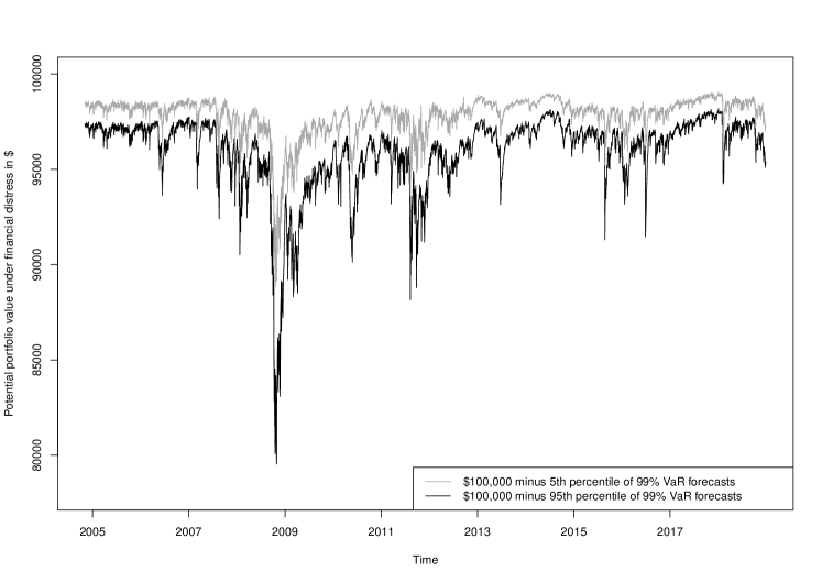
Figure 3: Average model risk for all groups

This figure shows the average model risk associated with one day ahead 99% VaR (first panel) and 97.5% ES (second panel) forecasts for a well diversified portfolio per group. Group 1 (G1) includes all model sets in which a copula function is fixed while varying the marginal distribution. Group 2 (G2) contains analogously the model sets with fixed marginal distribution and varying copula. Group 3 (G3) consists of all multivariate and Group 4 (G4) of all univariate models. Model risk is measured in terms of the mean absolute deviation (mad) of one day ahead forecasts by various risk models within a model set. Values are calculated on a daily basis between November 4, 2004 until December 31, 2018 in percent of the portfolio value based on all models that passed the respective backtest, see Section 2.2 for details.

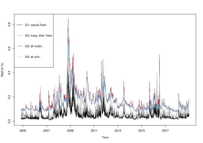
1 Average model risk (99% VaR)

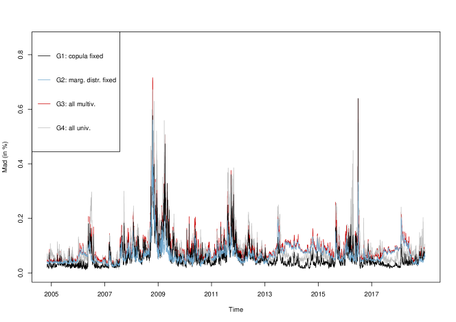
2 Average model risk (97.5% ES)

Figure 4: Potential portfolio value under financial distress based on the 99% VaR for fixed copula functions

This figure illustrates the economic significance of model risk arising from the choice of the GARCH-type model and marginal distribution. Here, we focus on the 99% VaR for model sets with fixed copula functions and varying univariate marginal distributions for a well diversified portfolio ($100,000) and a 10 day holding period. We provide the portfolio value minus the 20th and the 80th percentile of VaR forecasts from all models within each model set that passed the duration-based backtest by Christoffersen (2004) on a daily basis. Values are averaged over various copula specifications. This corresponds to the potential portfolio value under financial distress according to the more (80th percentile) or less (20th percentile) conservative VaR models. The sample period is November 4, 2004 until December 31, 2018.

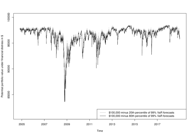
Figure 5: Potential portfolio value under financial distress based on the 99% VaR for fixed marginal distributions

This figure illustrates the economic significance of model risk arising from the choice of the copula function. Here, we focus on the 99% VaR for model sets with fixed univariate marginal distribution and varying copula functions for a well diversified portfolio ($100,000) and a 10 day holding period. We provide the portfolio value minus the 20th and the 80th percentile of VaR forecasts from all models within each model set that passed the duration-based backtest by Christoffersen (2004) on a daily basis. Values are averaged over various marginal distributions. This corresponds to the potential portfolio value under financial distress according to the more (80th percentile) or less (20th percentile) conservative VaR models. The sample period is November 4, 2004 until December 31, 2018.

Figure 6: Model risk of the VaR before and after applying the MCS procedure

This figure compares the model risk associated with one day ahead 99% VaR forecasts before and after applying the MCS procedure by Hansen et al. (2011). Model risk is measured in terms of the mean absolute deviation (mad) of risk forecasts by all multivariate VaR models that passed the duration-based test by Christoffersen (2004) (no MCS). Subsequently, we apply the MCS procedure to those models and recalculate model risk (MCS). Details on the method and its implementation can be found in Sections 2.4 and 5, respectively. Values are given in percent of the portfolio value between November 4, 2004 and December 31, 2018.

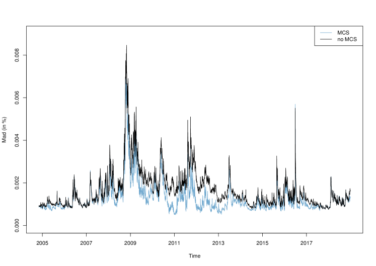
Figure 7: Number of VaR models before and after applying the MCS procedure

This figure shows the number of 99% VaR models before and after applying the MCS procedure by Hansen et al. (2011), see Section 2.4. In both cases, only those models (out of 180) that were not rejected by the duration-based VaR backtest by Christoffersen (2004) enter into the MCS procedure. The sample period is November 4, 2004 until December 31, 2018.

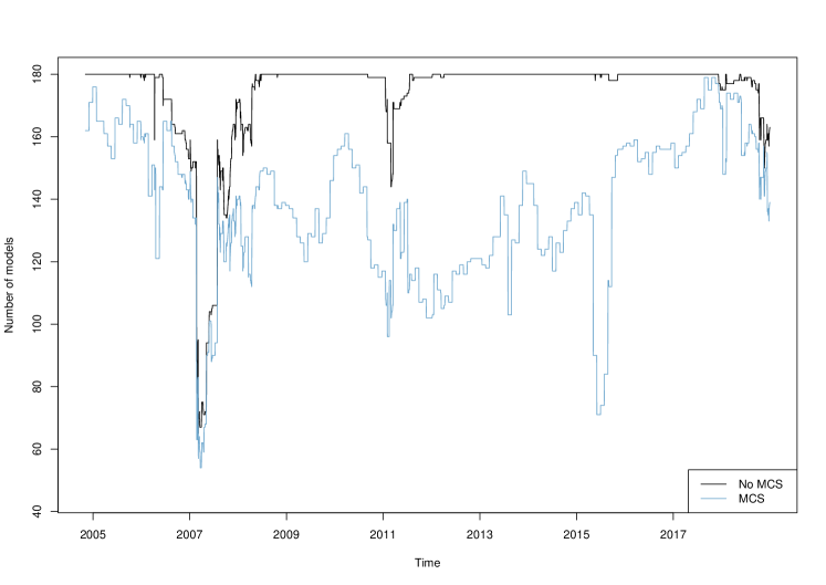
Figure 8: Number of market risk models passing the backtest

This figure shows the daily number of multivariate market risk models passing the respective backtest, see Section 2.2 for details. We consider risk forecasts associated with the one day ahead 99% VaR and 97.5% ES for a well diversified portfolio from November 4, 2004 to December 31, 2018.

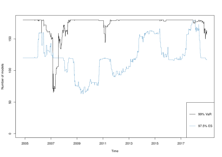
Figure 9: Average model risk without applying backtests (model sets with fixed and varying copula only)

This figure shows the average model risk associated with one day ahead 99% VaR (first panel) and 97.5% ES (second panel) forecasts for a well diversified portfolio per group. Group 1 (G1) includes all model sets in which a copula function is fixed while varying the marginal distribution. Group 2 (G2) contains analogously the model sets with fixed marginal distribution and varying copula. Model risk is measured in terms of the mean absolute deviation (mad) of one day ahead forecasts by various risk models within a model set. Values are calculated on a daily basis between November 4, 2004 until December 31, 2018 in percent of the portfolio value. In contrast to our baseline analysis, the models did not have to pass a backtest.

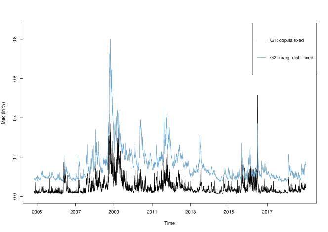
1 Average model risk (99% VaR)

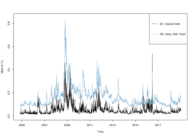
2 Average model risk (97.5% ES)

Table I: Summary statistics of index and portfolio returns

The table provides summary statistics for the returns of the indices that form the basis of our well-diversified portfolio as well as for the resulting portfolio returns with equal weighting. We include equity indices (developed and emerging markets), bond indices (governement, corporate, and high-yield bonds), a commodity index, and a real estate index. We retrieve the total return indices (in $) from Datastream for a period from January 2001 to December 2018. We first calculate geometric returns and derive equally weighted portfolio returns next. This corresponds to a portfolio consisting of 40% stocks, 40% bonds, 10% commodities and 10% real estate. We provide minimum (Min), median, mean, maximum (Max), and standard deviation (SD) of daily returns in percent as well as the kurtosis and skewness of the time series.

	Min	Median	Mean	Max	SD	Kurtosis	Skewness
	(in %)	(in %)	(in %)	(in %)	(in %)
Indices
Stoxx Europe 600	-9.691	0.042	0.024	11.284	1.341	10.642	-0.004
Dow Jones Industrial Average	-7.873	0.033	0.032	11.080	1.107	12.686	0.100
FTSE Developed Asia Pacific Index	-8.524	0.047	0.024	9.928	1.185	8.097	-0.262
MSCI Emerging Markets Index	-9.484	0.095	0.040	10.598	1.178	11.372	-0.306
S&P U.S. Treasury Bond Index	-1.658	0.012	0.014	1.758	0.232	5.995	-0.120
S&P 500 Investment Grade Corporate Bond Index	-1.668	0.027	0.020	1.845	0.284	5.028	-0.232
S&P U.S. High Yield Corporate Bond Index	-3.715	0.042	0.027	2.226	0.246	32.336	-2.377
S&P Pan-Europe Developed Sovereign Bond Index	-3.705	0.020	0.021	5.028	0.617	5.897	0.138
S&P GSCI	-8.762	0.000	-0.003	7.483	1.434	5.787	-0.148
Developed Markets Datastream Real Estate Index	-6.849	0.061	0.036	7.223	0.939	11.411	-0.370
Equally weighted portfolio	-4.009	0.042	0.023	4.110	0.552	11.085	-0.516

Table II: Model risk and the great financial crisis

This table presents summary statistics for the time series of model risk associated with 99% VaR and 97.5% ES forecasts for a well diversified portfolio. Model risk is measured in terms of the mean absolute deviation (mad) of risk forecasts by various models from November 4, 2004 until December 31, 2018. With crisis we refer to the years 2008-2009 while pre-crisis and after-crisis denote the period before and after, respectively. Model risk is calculated based on all multivariate models that passed the respective backtest, see Section 2.2 for details. We report model risk estimates for one day ahead risk forecasts in percent of the portfolio value (first and second column) and in absolute terms (third and fourth column) for an equally weighted portfolio. The results in absolute terms are based on a portfolio value of $100,000 and a 10 day forecast horizon obtained by applying the square-root-of-time rule. We provide minimum (Min), median, mean, maximum (Max), and standard deviation (SD) of the daily model risk estimates. Further results for randomly generated portfolio weights as well as alternative measures of model risk can be found in Tables III and IV.

		Model risk (in %)		Model risk (in $)
		99% VaR	97.5% ES	99% VaR	97.5% ES
Whole period	Min	0.075	0.029	237	92
	Median	0.138	0.080	436	253
	Mean	0.165	0.092	522	291
	Max	0.847	0.716	2,678	2,264
	SD	0.091	0.056	288	177
Pre-crisis	Min	0.081	0.029	256	92
	Median	0.105	0.050	332	158
	Mean	0.119	0.063	376	199
	Max	0.280	0.207	885	655
	SD	0.036	0.030	114	95
Crisis	Min	0.116	0.046	367	145
	Median	0.241	0.108	762	342
	Mean	0.286	0.145	904	459
	Max	0.847	0.716	2,678	2,264
	SD	0.139	0.101	440	319
Post-crisis	Min	0.075	0.034	237	108
	Median	0.138	0.082	436	259
	Mean	0.155	0.090	490	285
	Max	0.551	0.638	1,742	2,018
	SD	0.064	0.037	202	117

Table III: Model risk for all multivariate models averaged over 100 random portfolios

This table provides the same results as Table II but for 100 random portfolios obtained by drawing portfolio weights from a unit-simplex. Therefore, we first calculate summary statistics for the time series of model risk for each of the portfolios. These statistics are then averaged over all 100 portfolios. The results can thus be interpreted as summary statistics for the model risk of an average portfolio.

		Model risk (in %)		Model risk (in $)
		99% VaR	97.5% ES	99% VaR	97.5% ES
Whole period	Min	0.065	0.034	206	106
	Median	0.127	0.085	401	268
	Mean	0.153	0.099	484	313
	Max	0.813	0.763	2570	2413
	SD	0.086	0.057	272	181
Pre-crisis	Min	0.069	0.037	218	118
	Median	0.097	0.064	307	203
	Mean	0.111	0.074	351	233
	Max	0.281	0.233	890	735
	SD	0.036	0.029	113	91
Crisis	Min	0.108	0.046	342	146
	Median	0.221	0.114	697	361
	Mean	0.267	0.153	843	483
	Max	0.807	0.711	2551	2249
	SD	0.133	0.105	420	331
Post-crisis	Min	0.069	0.039	217	123
	Median	0.127	0.087	401	276
	Mean	0.143	0.096	451	303
	Max	0.593	0.626	1876	1980
	SD	0.060	0.039	189	123

Table IV: Alternative measures of model risk

This table provides summary statistics for different measures of model risk for 99% VaR and 97.5% forecasts. Our baseline measure is the mean absolute deviation (mad). We additionally include the standard deviation (sd) and interquartile range (iqr) of the risk forecasts by various models in percent of the portfolio value, see Section 2.3 for more details. Model risk is calculated for all multivariate models that passed the respective backtest. We provide minimum (Min), median, mean, maximum (Max), and standard deviation (SD) of the daily model risk estimates (according to the different model risk measures) over the period November 4, 2004 until December 31, 2018.

		Model risk
		Min	Median	Mean	Max	SD
	Measure
VaR	mad (in %)	0.075	0.138	0.165	0.847	0.091
	sd (in %)	0.088	0.161	0.195	0.992	0.108
	iqr (in %)	0.130	0.269	0.325	1.631	0.180
ES	mad (in %)	0.029	0.080	0.092	0.716	0.056
	sd (in %)	0.037	0.099	0.117	0.867	0.072
	iqr (in %)	0.040	0.133	0.152	1.399	0.094

Table V: Summary statistics of average model risk for all groups

This table presents summary statistics for the time series of average model risk associated with 99% VaR (Panel A) and 97.5% ES (Panel B) forecasts for a well diversified portfolio per group. Model risk is measured in terms of the mean absolute deviation (mad) of risk forecasts by various models within a model set from November 4, 2004 until December 31, 2018. All models passed the respective backtest, see Section 2.2 for details. Group 1 (G1) includes all model sets in which a copula function is fixed while varying the marginal distribution. Group 2 (G2) contains analogously the model sets with fixed marginal distribution and varying copula. Group 3 (G3) consists of all multivariate and Group 4 (G4) of all univariate models. We report model risk estimates for one day ahead risk forecasts in percent of the portfolio value (columns 1-5) and in absolute terms (column 6) for an equally weighted portfolio. The results in absolute terms are based on a portfolio value of $100,000 and a 10 day forecast horizon obtained by applying the square-root-of-time rule. We provide minimum (Min), median, mean, maximum (Max), and standard deviation (SD) of the daily averaged model risk estimates per group. Further results for randomly generated portfolio weights, various VaR and ES confidence levels as well as alternative measures of model risk (Groups 1 and 2 only) can be found in Tables VI, VIII, and VII. *** denotes a statistically significant increase in average model risk at the 1% level compared to Group 1.

Panel A: 99% VaR
	Average model risk (in %)						Average model risk (in $)
	Min	Median	Mean	Max	SD		Mean
Group
G1: copula fixed	0.008	0.037	0.052	0.518	0.044		164
G2: marg. distr. fixed	0.073	0.130	0.157***	0.803	0.084		498
G3: all multivariate	0.075	0.138	0.165	0.847	0.091		523
G4: all univariate	0.011	0.065	0.085	0.651	0.069		269
Panel B: 97.5% ES
	Average model risk (in %)						Average model risk (in $)
	Min	Median	Mean	Max	SD		Mean
Group
G1: copula fixed	0.012	0.042	0.058	0.640	0.049		184
G2: marg. distr. fixed	0.022	0.061	0.068***	0.561	0.036		216
G3: all multivariate	0.029	0.080	0.092	0.716	0.056		290
G4: all univariate	0.013	0.070	0.090	0.672	0.070		285

Table VI: Summary statistics of average model risk for all groups over 100 random portfolios

This table presents summary statistics for the time series of average model risk per group associated with 99% VaR (Panel A) and 97.5% ES (Panel B) forecasts for 100 random portfolios obtained by drawing portfolio weights from a unit-simplex. Therefore, we first calculate summary statistics for the time series of model risk for each of the portfolios. These statistics are then averaged over all 100 portfolios. The results can thus be interpreted as summary statistics for the model risk of an average portfolio. Model risk is measured in terms of the mean absolute deviation (mad) of risk forecasts by various models within a model set from November 4, 2004 until December 31, 2018. All models passed the respective backtest, see Section 2.2 for details. Group 1 (G1) includes all model sets in which a copula function is fixed while varying the marginal distribution. Group 2 (G2) contains analogously the model sets with fixed marginal distribution and varying copula. Group 3 (G3) consists of all multivariate and Group 4 (G4) of all univariate models. We report model risk estimates for one day ahead risk forecasts in percent of the portfolio value. We provide minimum (Min), median, mean, maximum (Max) and standard deviation (SD) of the daily averaged model risk estimates per group. *** denotes a statistically significant increase in average model risk at the 1% level compared to Group 1.

Panel A: 99% VaR
	Average model risk (mad in %)
	Min	Median	Mean	Max	SD
Group
G1: copula fixed	0.013	0.041	0.057	0.588	0.048
G2: marg. distr. fixed	0.056	0.118	0.142***	0.753	0.078
G3: all multivariate	0.065	0.127	0.153	0.813	0.086
G4: all univariate	0.012	0.066	0.087	0.751	0.071
Panel B: 97.5% ES
	Average model risk (mad in %)
	Min	Median	Mean	Max	SD
Group
G1: copula fixed	0.013	0.045	0.062	0.692	0.052
G2: marg. distr. fixed	0.024	0.069	0.075***	0.485	0.035
G3: all multivariate	0.034	0.085	0.099	0.763	0.057
G4: all univariate	0.015	0.071	0.093	0.762	0.072

Table VII: Summary statistics of average model risk for alternative model risk measures (model sets with fixed and varying copula only)

This table presents summary statistics for the time series of average model risk associated with 99% VaR (Panel A) and 97.5% ES (Panel B) forecasts for a well diversified portfolio per group. Model risk is captured by different measures based on risk forecasts by various models within a model set from November 4, 2004 until December 31, 2018. All models passed the respective backtest, see Section 2.2 for details. Our baseline measure is the mean absolute deviation (mad). We additionally include the standard deviation (sd) and interquartile range (iqr), see Section 2.3 for more details. Group 1 (G1) includes all model sets in which a copula function is fixed while varying the marginal distribution. Group 2 (G2) contains analogously the model sets with fixed marginal distribution and varying copula. We report model risk estimates for one day ahead risk forecasts in percent of the portfolio value. We provide minimum (Min), median, mean, maximum (Max) and standard deviation (SD) of the daily averaged model risk estimates per group. *** (**) denotes a statistically significant increase in average model risk at the 1% (5%) level compared to Group 1.

Panel A: 99% VaR
		Average model risk (in %)
		Min	Median	Mean	Max	SD
Group	Measure
G1: Copula fixed	mad	0.008	0.037	0.052	0.518	0.044
G1: Copula fixed	sd	0.016	0.048	0.069	0.636	0.063
G1: Copula fixed	iqr	0.011	0.057	0.075	0.869	0.060
G2: Marg. distr. fixed	mad	0.073	0.130	0.157***	0.803	0.084
G2: Marg. distr. fixed	sd	0.089	0.158	0.191***	0.975	0.101
G2: Marg. distr. fixed	iqr	0.103	0.255	0.311***	1.631	0.181
Panel B: 97.5% ES
		Average model risk (in %)
		Min	Median	Mean	Max	SD
Group	Measure
G1: Copula fixed	mad	0.012	0.042	0.058	0.640	0.049
G1: Copula fixed	sd	0.015	0.055	0.077	0.734	0.067
G1: Copula fixed	iqr	0.017	0.065	0.085	1.261	0.068
G2: Marg. distr. fixed	mad	0.022	0.061	0.068***	0.561	0.036
G2: Marg. distr. fixed	sd	0.031	0.081	0.090***	0.720	0.046
G2: Marg. distr. fixed	iqr	0.023	0.080	0.094**	0.857	0.057

Table VIII: Summary statistics of average model risk for all groups under various confidence levels

This table presents summary statistics for the time series of average model risk associated with 99.9%, 99%, 97.5% and 95% VaR (Panel A) and 99.9%, 99%, 97.5% and 95% ES (Panel B) forecasts for a well diversified portfolio per group. Model risk is measured in terms of the mean absolute deviation (mad) of risk forecasts by various models within a model set from November 4, 2004 until December 31, 2018. All models passed the respective backtest, see Section 2.2 for details. Group 1 (G1) includes all model sets in which a copula function is fixed while varying the marginal distribution. Group 2 (G2) contains analogously the model sets with fixed marginal distribution and varying copula. Group 3 (G3) consists of all multivariate and Group 4 (G4) of all univariate models. We report model risk estimates for one day ahead risk forecasts in percent of the portfolio value. We provide minimum (Min), median, mean, maximum (Max) and standard deviation (SD) of the daily averaged model risk estimates per group. *** denotes a statistically significant increase in average model risk at the 1% level compared to Group 1.

Panel A: VaR								Panel B: ES
		Average model risk (mad in %)								Average model risk (mad in %)
		Min	Median	Mean	Max	SD				Min	Median	Mean	Max	SD
Conf. level	Group							Conf. level	Group
99.9%	G1: copula fixed	0.031	0.088	0.108	0.747	0.070		99.9%	G1: copula fixed	0.023	0.119	0.136	0.875	0.083
	G2: marg. distr. fixed	0.122	0.248	0.293***	1.507	0.156			G2: marg. distr. fixed	0.054	0.245	0.270***	1.435	0.125
	G3: all multivariate	0.127	0.261	0.306	1.553	0.162			G3: all multivariate	0.068	0.279	0.309	1.506	0.139
	G4: all univariate	0.031	0.169	0.197	1.454	0.124			G4: all univariate	0.000	0.221	0.244	1.521	0.161
99.0%	G1: copula fixed	0.008	0.037	0.052	0.518	0.044		99.0%	G1: copula fixed	0.019	0.060	0.079	0.731	0.062
	G2: marg. distr. fixed	0.073	0.130	0.157***	0.803	0.084			G2: marg. distr. fixed	0.047	0.105	0.117***	0.682	0.054
	G3: all multivariate	0.075	0.138	0.165	0.847	0.091			G3: all multivariate	0.056	0.124	0.142	0.820	0.073
	G4: all univariate	0.011	0.065	0.085	0.651	0.069			G4: all univariate	0.017	0.104	0.126	0.848	0.085
97.5%	G1: copula fixed	0.007	0.028	0.040	0.391	0.036		97.5%	G1: copula fixed	0.012	0.042	0.058	0.640	0.049
	G2: marg. distr. fixed	0.049	0.090	0.109***	0.581	0.061			G2: marg. distr. fixed	0.022	0.061	0.068***	0.561	0.036
	G3: all multivariate	0.050	0.097	0.117	0.626	0.067			G3: all multivariate	0.029	0.080	0.092	0.716	0.056
	G4: all univariate	0.009	0.045	0.062	0.506	0.056			G4: all univariate	0.013	0.070	0.090	0.672	0.070
95.0%	G1: copula fixed	0.006	0.023	0.034	0.308	0.031		95.0%	G1: copula fixed	0.008	0.033	0.045	0.543	0.039
	G2: marg. distr. fixed	0.032	0.065	0.078***	0.453	0.047			G2: marg. distr. fixed	0.012	0.041	0.045	0.369	0.025
	G3: all multivariate	0.032	0.070	0.085	0.484	0.054			G3: all multivariate	0.018	0.058	0.067	0.651	0.044
	G4: all univariate	0.006	0.035	0.050	0.412	0.046			G4: all univariate	0.009	0.052	0.069	0.521	0.059

Table IX: Model risk before and after applying the MCS procedure

This table compares the model risk associated with one day ahead forecasts of the 99% VaR and the 97.5% ES before and after applying the model confidence set (MCS) procedure by Hansen et al. (2011). Details on the method and its implementation can be found in Sections 2.4 and 5, respectively. Model risk is measured in terms of the mean absolute deviation (mad) of risk forecasts by various models in percent of the portfolio value. Model risk is calculated on a daily basis from November 4, 2004 until December 31, 2018 for all multivariate models that passed the respective backtest. The term crisis refers to the years 2008-2009 while pre-crisis and after-crisis denote to the period before and after, respectively. We provide minimum (Min), median, mean, maximum (Max) and standard deviation (SD) of the daily model risk estimates. *** denotes statistically significant reductions of mean model risk at the 1% level by applying the MCS procedure.

		No MCS		MCS
		Model risk (in %)		Model risk (in %)
		99% VaR	97.5% ES	99% VaR	97.5% ES
Whole period	Min	0.075	0.029	0.051	0.022
	Median	0.138	0.080	0.106	0.078
	Mean	0.165	0.092	0.127***	0.089***
	Max	0.847	0.716	0.696	0.703
	SD	0.091	0.056	0.070	0.054
Pre-crisis	Min	0.081	0.029	0.069	0.022
	Median	0.105	0.050	0.098	0.049
	Mean	0.119	0.063	0.110***	0.062***
	Max	0.280	0.207	0.259	0.214
	SD	0.036	0.030	0.034	0.030
Crisis	Min	0.116	0.046	0.087	0.045
	Median	0.241	0.108	0.172	0.099
	Mean	0.286	0.145	0.215***	0.138***
	Max	0.847	0.716	0.696	0.703
	SD	0.139	0.101	0.120	0.097
Post-crisis	Min	0.075	0.034	0.051	0.034
	Median	0.138	0.082	0.099	0.081
	Mean	0.155	0.090	0.113***	0.088***
	Max	0.551	0.638	0.569	0.647
	SD	0.064	0.037	0.045	0.037

Table X: Summary statistics of market risk models passing the backtest

This table presents summary statistics on the number of multivariate market risk models passing the respective backtest, see Section 2.2 for details. We consider VaR (Panel A) and ES (Panel B) forecasts for a well diversified portfolio from November 4, 2004 until December 31, 2018 and confidence levels (Conf. level) ranging from 95% to 99.9%. We provide minimum (Min), median, mean, maximum (Max) and standard deviation (SD) of the daily number of models.

Panel A: VaR
	Models passing backtest
	Min	Median	Mean	Max	SD
Conf. level
99.9%	137	180	178	180	5
99.0%	65	180	174	180	17
97.5%	89	180	176	180	11
95.0%	158	180	179	180	3
Panel B: ES
	Models passing backtest
	Min	Median	Mean	Max	SD
Conf. level
99.9%	45	113	123	180	46
99.0%	97	130	136	180	25
97.5%	63	120	121	179	27
95.0%	24	119	109	168	31

Table XI: Summary statistics of market risk models passing alternative backtests

This table presents summary statistics on the number of multivariate market risk models passing a set of backtesting alternatives. For our main analysis, we rely on the duration-based VaR backtest by Christoffersen (2004) and the conditional calibration ES backtest by Nolde and Ziegel (2017) with a moving window of 500 days (Baseline). For robustness, we also consider the dynamic quantile VaR backtest by Engle and Manganelli (2004) and the exceedance residual ES backtest by McNeil and Frey (2000) (Alternative backtests), for more details we refer to Section 2.2. Additionally, we provide results when not applying any backtest (No backtest) or when using the baseline backtest with a fixed window (Fixed window) or a moving window of 1000 days (1000 days mov. window). We consider VaR (Panel A) and ES (Panel B) forecasts for a well diversified portfolio from November 4, 2004 until December 31, 2018 and confidence levels (Conf. level) ranging from 95% to 99.9%. We provide minimum (Min), median, mean, maximum (Max) and standard deviation (SD) of the daily number of models.

Panel A: 99% VaR
	Models passing backtest
	Min	Median	Mean	Max	SD
Baseline	65	180	174	180	17
No backtest	180	180	180	180	0
Alternative backtest	0	65	71	160	42
Fixed window	113	113	113	113	0
1000 days mov. window	0	179	145	180	62
Panel B: 97.5% ES
	Models passing backtest
	Min	Median	Mean	Max	SD
Baseline	63	120	121	179	27
No backtest	180	180	180	180	0
Alternative backtest	99	119	127	180	21
Fixed window	17	17	17	17	0
1000 days mov. window	0	95	82	120	39

Table XII: Model risk and alternative backtests (all multivariate models)

This table provides summary statistics on the model risk associated with one day ahead forecasts of 99% VaR and 97.5% ES after having different (or differently specified) backtests. For our main analysis, we rely on the duration-based VaR backtest by Christoffersen (2004) and the conditional calibration ES backtest by Nolde and Ziegel (2017) with a moving window of 500 days (Baseline). For robustness, we also consider the dynamic quantile VaR backtest by Engle and Manganelli (2004) and the exceedance residual ES backtest by McNeil and Frey (2000) (Alternative backtests), for more details we refer to Section 2.2. Additionally, we provide results when not applying any backtest (No backtest) or when using the baseline backtest with a fixed window (Fixed window) or a moving window of 1000 days (1000 days mov. window).
Model risk is measured in terms of the mean absolute deviation (mad) of the risk forecasts that passed the respective backtest on a daily basis from November 4, 2004 until December 31, 2018. We report model risk estimates in percent of the portfolio value (first and second column) and in absolute terms (third and fourth column) for an equally weighted portfolio. The results in absolute terms are based on a portfolio value of $100,000 and a 10 day forecast horizon. We provide minimum (Min), median, mean, maximum (Max), and standard deviation (SD) of the daily model risk estimates.

			Model risk (in %)		Model risk (in $)
			99% VaR	97.5% ES	99% VaR	97.5% ES
	Baseline	Min	0.075	0.029	237	92
		Median	0.138	0.080	436	253
		Mean	0.165	0.092	522	291
		Max	0.847	0.716	2,678	2,264
		SD	0.091	0.056	288	177
	No backtest	Min	0.056	0.058	177	183
		Median	0.127	0.133	402	421
		Mean	0.156	0.163	493	515
		Max	0.847	0.876	2678	2770
		SD	0.089	0.092	281	291
Alternative	backtests	Min	0.000	0.032	0	101
		Median	0.065	0.095	206	300
		Mean	0.079	0.114	250	360
		Max	0.672	0.864	2125	2732
		SD	0.054	0.077	171	243
Fixed	window	Min	0.035	0.011	111	35
		Median	0.097	0.068	307	215
		Mean	0.129	0.078	408	247
		Max	1.081	0.712	3418	2252
		SD	0.103	0.049	326	155
1000 days	mov. window	Min	0.048	0.025	152	79
		Median	0.170	0.072	538	228
		Mean	0.202	0.091	639	288
		Max	1.118	0.962	3535	3042
		SD	0.113	0.067	357	212

Table XIII: Model risk and alternative backtests (model sets with fixed and varying copula only)

This table presents summary statistics for the time series of average model risk per group associated with 99% VaR (Panel A) and 97.5% ES (Panel B) forecasts for a well diversified portfolio and a set of backtesting alternatives. For our main analysis, we rely on the duration-based VaR backtest by Christoffersen (2004) and the conditional calibration ES backtest by Nolde and Ziegel (2017) with a moving window of 500 days (Baseline). For robustness, we also consider the dynamic quantile VaR backtest by Engle and Manganelli (2004) and the exceedance residual ES backtest by McNeil and Frey (2000) (Alternative backtests), for more details we refer to Section 2.2. Additionally, we provide results when not applying any backtest (No backtest) or when using the baseline backtest with a fixed window (Fixed window) or a moving window of 1000 days (1000 days mov. window). Model risk is measured in terms of the mean absolute deviation (mad) of risk forecasts by various models within a model set that passed the respective backtest on a daily basis from November 4, 2004 until December 31, 2018. Group 1 (G1) includes all model sets in which a copula function is fixed while varying the marginal distribution. Group 2 (G2) contains analogously the model sets with fixed marginal distribution and varying copula. We report model risk estimates for one day ahead risk forecasts in percent of the portfolio value. We provide minimum (Min), median, mean, maximum (Max), and standard deviation (SD) of the daily averaged model risk estimates per group.

Panel A: 99% VaR
		Average model risk (in %)
		Min	Median	Mean	Max	SD
Group
G1: Copula fixed	Baseline	0.008	0.037	0.052	0.518	0.044
	No backtest	0.012	0.037	0.052	0.518	0.044
	Alternative backtest	0.000	0.039	0.051	0.524	0.041
	Fixed window	0.011	0.033	0.048	0.516	0.043
	1000 days mov. window	0.014	0.040	0.053	0.518	0.041
G2: Marg. distr. fixed	Baseline	0.073	0.130	0.157	0.803	0.084
	No backtest	0.075	0.130	0.157	0.803	0.084
	Alternative backtest	0.000	0.038	0.042	0.439	0.024
	Fixed window	0.058	0.103	0.126	0.717	0.072
	1000 days mov. window	0.075	0.137	0.159	0.669	0.073
Panel B: 97.5% ES
		Average model risk (in %)
		Min	Median	Mean	Max	SD
Group
G1: Copula fixed	Baseline	0.012	0.042	0.058	0.640	0.049
	No backtest	0.012	0.040	0.055	0.537	0.045
	Alternative backtest	0.012	0.042	0.058	0.581	0.050
	Fixed window	0.006	0.027	0.039	0.546	0.039
	1000 days mov. window	0.017	0.047	0.065	0.640	0.053
G2: Marg. distr. fixed	Baseline	0.022	0.061	0.068	0.561	0.036
	No backtest	0.080	0.137	0.164	0.835	0.087
	Alternative backtest	0.029	0.069	0.077	0.561	0.045
	Fixed window	0.003	0.029	0.034	0.423	0.026
	1000 days mov. window	0.015	0.039	0.047	0.546	0.035

This Internet Appendix contains theoretical foundations as well as several additional tables and figures that complement the results presented in the main paper.

IA.1 Theoretical foundations

IA.1.1 ARMA-GARCH process

In an ARMA(p,q)-GARCH(r,s) process, the conditional mean of a (univariate) time series is modeled by the ARMA part while the conditional volatility is captured by the GARCH part. With ARMA(p,q) we denote a model with $p$ autoregressive and $q$ moving average terms. More formally, we have the following specification

$$r_{t}=\mu+\sum_{j=1}^{p}\phi_{j}r_{t-j}+\sum_{j=1}^{q}\theta_{j}\epsilon_{t-j}+\epsilon_{t},$$

where $r_{\tau},\tau=t-p,\dots,t$ are observations from the time series and $\phi_{j},j=1,\dots,p$, $\theta_{j},j=1,\dots,q$, and $\mu$ denote parameters. The Generalized Autoregressive Conditional Heteroskedasticity (GARCH) model by Bollerslev (1986) extends the ARCH model due to Engle (1982) by including lags of the conditional variances. More exactly, the variance equation according to the GARCH(r,s) model at time $t$ is given by

$$\sigma_{t}^{2}=\omega+\sum_{j=1}^{r}\beta_{j}\sigma^{2}_{t-j}+\sum_{j=1}^{s}\alpha_{j}\epsilon^{2}_{t-j},$$

where $\sigma^{2}_{\tau},\tau=t-r,\dots,t$ denotes the conditional variance, $\alpha_{j},j=1,\dots,s$, $\beta_{j},j=1,\dots,r$, and $\omega$ are parameters and all $\epsilon_{t}$ are of the form $\epsilon_{t}=z_{t}\sigma_{t}$ where $z_{t}$ is an iid process with zero mean and unit variance. The parameters must fulfill some conditions in order to guarantee that the GARCH conditional variance estimates are always positive, see Nelson and Cao (1992) for details. In case of the GARCH(1,1) model, forecasts can be calculated as

$$\sigma^{2}_{t+h|t}=\sigma^{2}+(\alpha+\beta)^{h-1}(\sigma^{2}_{t+1}-\sigma^{2}),$$

where $h>2$ denotes the horizon of the forecasts and $\sigma^{2}$ denotes the unconditional variance given by $\sigma^{2}=\frac{\omega}{1-\alpha-\beta}$ (see Bollerslev, 2010).

IA.1.2 Sklar’s theorem

The popularity of copulas in multivariate dependence modeling is due to the theorem by Sklar (1959). Loosely speaking the theorem states that modeling of the marginals and of the multivariate dependence can be separated by means of copulas functions.

Theorem 1 (Sklar’s theorem)

Let $\mathbf{X}=(X_{1},\dots,X_{d})\sim F$ be a $d$-dimensional random variable with marginal distributions $F_{j},j=1,\dots,d.$ We then have

$$F(x_{1},\dots,x_{d})=C\big{(}F_{1}(x_{1}),\dots,F_{d}(x_{d})\big{)},$$

where $C$ denotes some appropriate $d$-dimensional copula. If the multivariate distribution function $F$ is absolutely continuous and the marginal distributions $F_{1},\dots,F_{d}$ are strictly increasing continuous, we have

$$f(x_{1},\dots,x_{d})=\Big{(}\prod_{j=1}^{d}f_{j}(x_{j})\Big{)}\cdot c\big{(}F_{1}(x_{1}),\dots,F_{d}(x_{d})\big{)}$$

with the small letters denoting the corresponding probability density functions.

The second part of the theorem highlights that the joint distribution of the random variable $\mathbf{X}$ can be modeled separately in terms of a “marginal term” $\prod_{j=1}^{d}f_{j}(x_{j})$ and a “dependence term” $c\big{(}F_{1}(x_{1}),\dots,F_{d}(x_{d})\big{)}$. The marginal term is based on information from the (univariate) marginals alone and does not contain any information about the multivariate dependence. On the other hand, the random variables $F_{1}(X_{1}),\dots,F_{d}(X_{d})$ are all uniformly distributed in the interval $[0,1]$ and therefore do not contain any information on the marginals. For more details we refer to the books by Joe (2001) and Nelsen (2006).

IA.1.3 Duration-based backtest

The duration-based VaR backtest by Christoffersen (2004), as the name implies, is based on the duration of days between VaR violations. The hit sequence of $VaR_{t}$ violations is defined as

$$I_{t}=\begin{cases}&1,\quad\text{if}~{}r_{t}<-VaR_{t}(p)\\ &0,\quad\text{else}\end{cases}$$

where $r_{t}$ is a time series of daily ex-post portfolio returns and $VaR_{t}(p)$ a time series of ex-ante VaR forecasts with a coverage rate $p$. The time in days between two VaR violations is called the no-hit duration $D_{i}=t_{i}-t_{i-1}$ where $t_{i}$ denotes the day of violation number $i$. The null hypothesis of the test is then: If the VaR model is correctly specified for coverage rate $p$, the no-hit duration or in other words the conditional expected duration between VaR violations should have no memory and a mean duration of $1/p$ days. Thus, under the null hypothesis the no-hit duration follows the exponential distribution

$$f_{exp}(D;p)=p~{}exp(-pD)$$

whereas the alternative that allows for duration dependence follows a Weibull distribution

$$f_{W}(D;a,b)=a^{b}bD^{b-1}exp(-(aD)^{b}).$$

The tested null hypothesis of independence is then defined as

$$H_{0,ind}:b=1.$$

For a detailed derivation of the no-memory property in terms of the discrete probability distribution and its hazard function, please see Christoffersen (2004).

IA.1.4 Conditional calibration backtest

Nolde and Ziegel (2017) introduce a conditional calibration (CC) test and show that well-known traditional backtests can be unified within the concept of CC. The CC test comes in two versions: The simple version used in our analysis requires only risk forecasts (VaR and ES), whereas the general version additionally needs information on conditional volatility. Following Nolde and Ziegel (2017), $\mathcal{P}_{0}$ defines the class of Borel-probability distributions on $\mathbb{R}$. Moreover, $\mathcal{P}_{1}\subseteq\mathcal{P}_{0}$ denotes the class of all distributions with finite mean whereas $\mathcal{P}_{V}\subset\mathcal{P}_{0}$ describes distributions with unique quantiles. The CC backtests rely on so-called identification functions. We further follow the notation of Nolde and Ziegel (2017) and define $\Theta=(\rho_{1},...,\rho_{k})$ as the identifiable functional with an identification function $V$ with respect to $\mathcal{P}$. Let $\{r_{t}\}_{t\in\mathbb{N}}$ be a series of negated log-returns that are adapted to the filtration $\mathcal{F}=\{\mathcal{F}_{t}\}_{t\in\mathbb{N}}$. Further, we define $\{x_{t}\}_{t\in\mathbb{N}}$ as a sequence of predictions of $\Theta$ that are $\mathcal{F}_{t-1}$-measurable. All conditional distributions $\mathcal{L}(r_{t}|\mathcal{F}_{t-1})$ and all unconditional distributions $\mathcal{L}(r_{t})$ are assumed to belong to $\mathcal{P}$ almost surely. The identification function used for the pair $(VaR_{\nu},ES_{\nu})$ for the level $\nu\in(0,1)$ is defined as

$$V(x_{1},x_{2},r)=\left(\frac{1-\nu-\mathbb{I}_{(0,\infty)}(r-x_{1})}{x_{1}-x_{2}-\frac{1}{1-\nu}\mathbb{I}_{(0,\infty)}(r-x_{1})(x_{1}-r)}\right)$$

with respect to $\mathcal{P}_{1}\cap\mathcal{P}_{V}$, where $\mathbb{I}_{(0,\infty)}$ denotes the characteristic function of the open interval $(0,\infty)$. The sequence of predictions $\{x_{t}\}_{t\in\mathbb{N}}$ is conditionally calibrated for $\Theta$ if

$$\mathbb{E}(V(x_{t},r_{t})|\mathcal{F}_{t-1})=0\quad\text{almost surely},\forall t\in\mathbb{N}.$$

The null hypothesis of the traditional backtest for CC considers exactly this requirement: The sequence of predictions $\{x_{t}\}_{t\in\mathbb{N}}$ is conditionally calibrated for $\Theta$. Here, the requirement for the expected value is equivalent to $\mathbb{E}(h^{{}^{\prime}}_{t}V(x_{t},r_{t}))=0$ for all $\mathcal{F}_{t-1}$-measurable $\mathbb{R}^{k}$-valued functions $h_{t}$. Nolde and Ziegel (2017) consider a $\mathcal{F}$-predictable sequence $\{\mathbf{h}_{t}\}_{t\in\mathbb{N}}$ of $q\times k$-matrices $\mathbf{h}_{t}$ called test functions to construct a Wald-type test statistic. For the simple version of the CC test, $\mathbf{h}_{t}$ equals the identity matrix. For more information on the Wald-type test statistic as well as a complete derivation of the CC test in both versions, please refer to the original paper.

IA.1.5 Model confidence set procedure

In this section we more formally introduce the MCS procedure outlined in Section 2.4. Let therefore $\mathcal{M}^{0}$ denote the set of candidate models, $\mathcal{M}^{*}$ the true set of best models, and $\hat{\mathcal{M}}^{*}_{1-\alpha}$ the model confidence set at confidence level $\alpha$. We further assume that $\mathcal{M}^{0}$ consists of a finite number $m_{0}$ of models. Based on an evaluation criterion (the loss function) one can calculate the losses $L_{i,t}$ that are associated with model $i$ at time $t$. In the case of a VaR forecast, e.g., one might compare the risk forecast $VaR_{\alpha}^{i,t}$ of model $i$ at time $t$ with the actual realized return $r_{t}$ by setting $L_{i,t}:=L(VaR_{\alpha}^{i,t},r_{t})$ where $L$ denotes an appropriate loss function. For $i,j\in\mathcal{M}^{0}$ one then defines the relative performance variable

$$d_{ij,t}:=L_{i,t}-L_{j,t}$$

as well as the expected value of the performance variable

$$\mu_{ij}:=E(d_{ij,t}).$$

The alternatives in $\mathcal{M}^{0}$ are now ranked based on their expected loss. That is, model $i$ is preferred over model $j$ if $\mu_{ij}<0.$ The MCS is now constructed based on a sequence of significance tests

$$H_{0,\mathcal{M}}:\mu_{ij}=0\quad\text{for all }i,j\in\mathcal{M},$$

with $\mathcal{M}\subseteq\mathcal{M}^{0}$. If $H_{0,\mathcal{M}}$ can be rejected, the elimination rule is applied to remove a model from $\mathcal{M}$ that is inferior to the remaining ones. The model confidence set is then defined as any subset of $\mathcal{M}^{0}$ that contains all best models with a given probability $1-\alpha$. More shortly, the MCS procedure can be summarized in the following algorithmic form (see Hansen et al., 2011):

Step 0: $$\text{Set }\mathcal{M}:=\mathcal{M}^{0}.$$

Step 1: $$\text{Test the null hypothesis }H_{0,\mathcal{M}}\text{ based on the equivalence test }\delta_{\mathcal{M}}\text{ at the confidence level }\alpha.$$

Step 2: $$\text{If }H_{0,\mathcal{M}}\text{ is not rejected, set }\hat{\mathcal{M}}^{*}_{1-\alpha}:=\mathcal{M}\text{, otherwise use the elimination rule }e_{\mathcal{M}}\text{ to elimi-}$$

$$\text{nate a model from }\mathcal{M}\text{ and repeat the procedure from step 1.}$$

Hansen et al. (2011) provide two t-statistics for the hypothesis test in step 1. We opt for the statistic $t_{ij}$ that is also used in the test for comparing two forecasts (see Diebold and Mariano, 1995; West, 1996). We therefore define the sample loss statistic $\bar{d}_{ij}:=\frac{1}{n}\sum_{t=1}^{n}d_{ij,t}$ and set

$$t_{ij}:=\frac{\bar{d}_{ij}}{\sqrt{\hat{var}(\bar{d}_{ij})}},$$

where $\hat{var}(\bar{d}_{ij})$ denotes an estimate of $var(\bar{d}_{ij})$. The final test statistic is then defined as

$$T_{R,\mathcal{M}}:=\max_{i,j\in\mathcal{M}}|t_{ij}|.$$

The asymptotic distribution of $T_{R,\mathcal{M}}$ is non-standard and derived via a bootstrapping scheme, see Hansen et al. (2011) for details. The natural elimination rule corresponding to the test statistic $T_{R,\mathcal{M}}$ is $e_{R,\mathcal{M}}:=\arg\max_{i\in\mathcal{M}}\sup_{j\in\mathcal{M}}t_{ij}$ because the corresponding model is such that $t_{e_{R,\mathcal{M}}j}=T_{R,\mathcal{M}}$ is fulfilled for some $j\in\mathcal{M}$. Removing model $e_{R,\mathcal{M}}$ will therefore reduce (or at least not increase) the test statistic $T_{R,\mathcal{M}}$.

IA.2 Figures

Figure IA.1: Potential portfolio value under financial distress according to the 97.5% ES

This figure illustrates the economic significance of model risk arising from the disparity between different ES models. Here, we focus on the 97.5% ES for a well diversified portfolio ($100,000) and a 10 day holding period between November 4, 2004 and December 31, 2018. We provide the portfolio value minus the 5th and the 95th percentile of ES forecasts from all multivariate models that passed the conditional calibration backtest by Nolde and Ziegel (2017) on a daily basis. This corresponds to the potential portfolio value under financial distress according to the more (95th percentile) or less (5th percentile) conservative ES models.

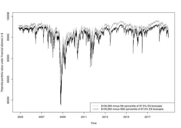
Figure IA.2: Average model risk for alternative model risk measures (model sets with fixed and varying copula only)

This figure shows the average model risk associated with one day ahead 99% VaR (Subfigures 1, 3, and 5) and 97.5% ES (Subfigures 2, 4, and 6) forecasts for a well diversified portfolio per group. Group 1 (G1) includes all model sets in which a copula function is fixed while varying the marginal distribution. Group 2 (G2) contains analogously the model sets with fixed marginal distribution and varying copula. Model risk is captured by different measures of one day ahead forecasts by various risk models within a model set. Our baseline measure is the mean absolute deviation (mad). We additionally include the standard deviation (sd) and interquartile range (iqr), see Section 2.3 for more details. Values are calculated on a daily basis between November 4, 2004 until December 31, 2018 in percent of the portfolio value based on all models that passed the respective backtest, see Section 2.2 for details.

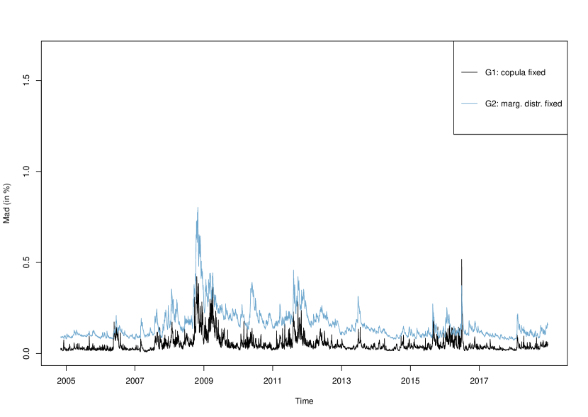
1 Average model risk (99% VaR) - mad

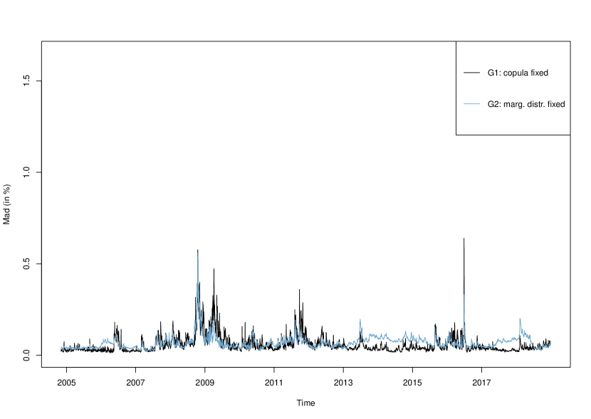
2 Average model risk (97.5% ES) - mad

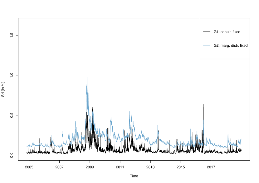
3 Average model risk (99% VaR) - sd

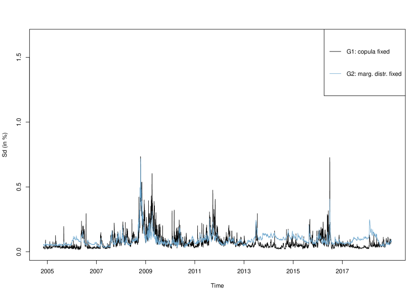
4 Average model risk (97.5% ES) - sd

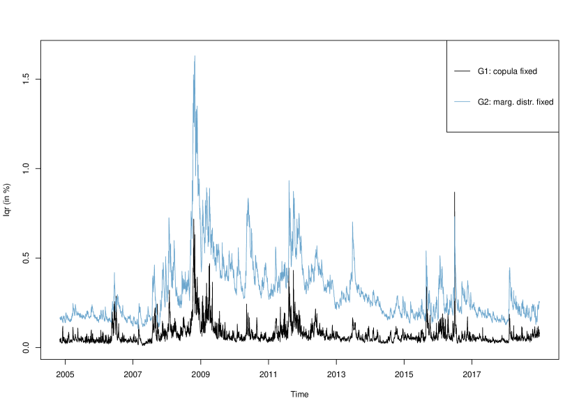
5 Average model risk (99% VaR) - iqr

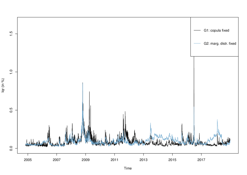
6 Average model risk (97.5% ES) - iqr

Figure IA.3: Average model risk for all groups under various VaR confidence levels

This figure shows the average model risk associated with one day ahead VaR forecasts for a well diversified portfolio and a confidence level of 99.9%, 99%, 97.5%, and 95% (Subfigures 1-4) per group. Group 1 (G1) includes all model sets in which a copula function is fixed while varying the marginal distribution. Group 2 (G2) contains analogously the model sets with fixed marginal distribution and varying copula. Group 3 (G3) consists of all multivariate and Group 4 (G4) of all univariate models. Model risk is measured in terms of the mean absolute deviation (mad) of one day ahead forecasts by various risk models within a model set. Values are calculated on a daily basis between November 4, 2004 until December 31, 2018 in percent of the portfolio value based on all models that passed the respective backtest, see Section 2.2 for details.

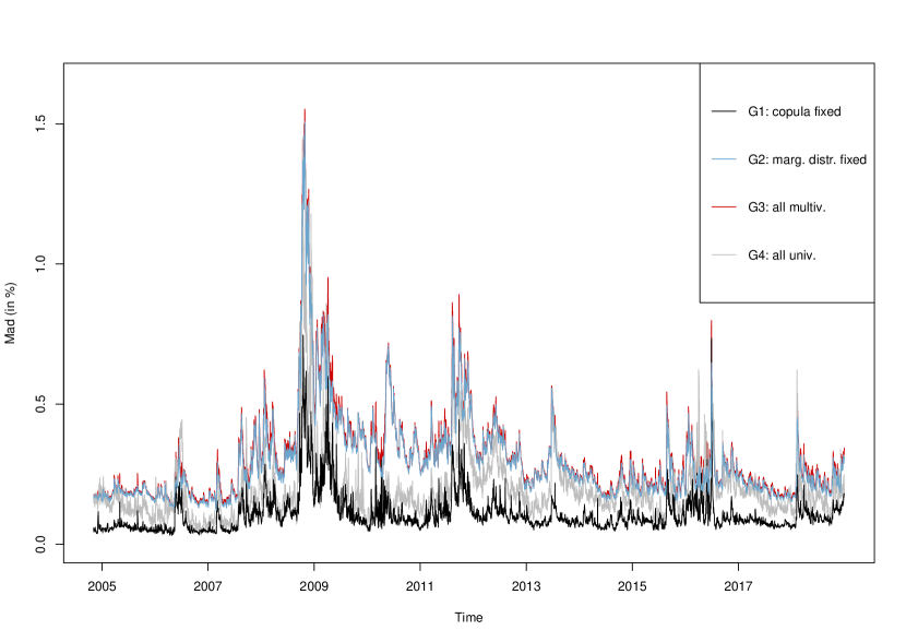
1 Average model risk (99.9% VaR)

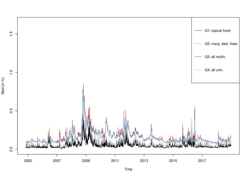
2 Average model risk (99% VaR)

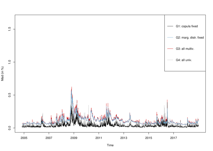
3 Average model risk (97.5% VaR)

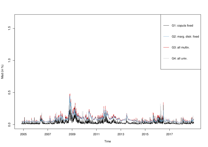
4 Average model risk (95% VaR)

Figure IA.4: Average model risk for all groups under various ES confidence levels

This figure shows the average model risk associated with one day ahead ES forecasts for a well diversified portfolio and a confidence level of 99.9%, 99%, 97.5%, and 95% (Subfigures 1-4) per group. Group 1 (G1) includes all model sets in which a copula function is fixed while varying the marginal distribution. Group 2 (G2) contains analogously the model sets with fixed marginal distribution and varying copula. Group 3 (G3) consists of all multivariate and Group 4 (G4) of all univariate models. Model risk is measured in terms of the mean absolute deviation (mad) of one day ahead forecasts by various risk models within a model set. Values are calculated on a daily basis between November 4, 2004 until December 31, 2018 in percent of the portfolio value based on all models that passed the respective backtest, see Section 2.2 for details.

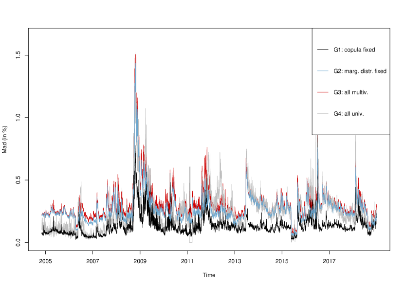
1 Average model risk (99.9% ES)

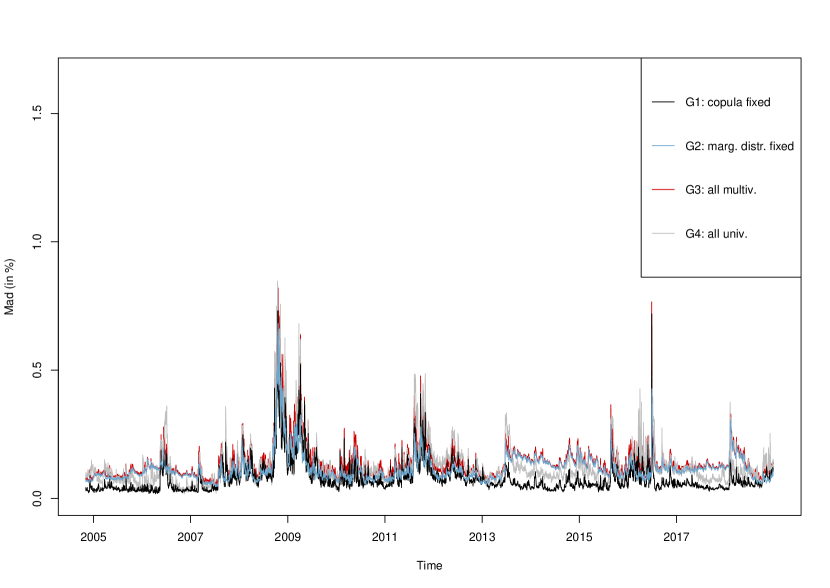
2 Average model risk (99% ES)

3 Average model risk (97.5% ES)

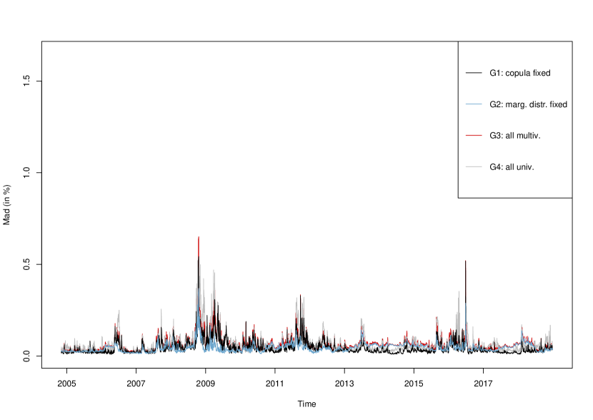
4 Average model risk (95% ES)

References

- Aas and Berg (2009) Aas, K. and D. Berg (2009): “Models for construction of multivariate dependence – a comparison study,” The European Journal of Finance, 15, 639–659.
- Aas et al. (2009) Aas, K., C. Czado, A. Frigessi, and H. Bakken (2009): “Pair-copula constructions of multiple dependence,” Insurance: Mathematics and Economics, 44, 182–198.
- Acerbi and Székely (2014) Acerbi, C. and B. Székely (2014): “Backtesting expected shortfall,” Risk, 76–81.
- Alexander and Sarabia (2012) Alexander, C. and J. M. Sarabia (2012): “Quantile uncertainty and value-at-risk model risk,” Risk Analysis, 32, 1293–1308.
- Ausin and Lopes (2010) Ausin, M. C. and H. F. Lopes (2010): “Time-varying joint distribution through copulas,” Computational Statistics & Data Analysis, 54, 2383–2399.
- Barendse et al. (2019) Barendse, S., E. Kole, and D. J. van Dijk (2019): “Backtesting Value-at-Risk and Expected Shortfall in the Presence of Estimation Error,” SSRN Electronic Journal.
- Basel Committee on Banking Supervision (2019) Basel Committee on Banking Supervision (2019): Minimum capital requirements for market risk, Basel: Basel Committee on Banking Supervision.
- Bassetti et al. (2018) Bassetti, F., M. E. De Giuli, E. Nicolino, and C. Tarantola (2018): “Multivariate dependence analysis via tree copula models: An application to one-year forward energy contracts,” European Journal of Operational Research, 269, 1107–1121.
- Bayer and Dimitriadis (2020a) Bayer, S. and T. Dimitriadis (2020a): “esback: Expected Shortfall Backtesting,” .
- Bayer and Dimitriadis (2020b) ——— (2020b): “Regression-Based Expected Shortfall Backtesting,” Journal of Financial Econometrics.
- Bedford and Cooke (2001) Bedford, T. and R. M. Cooke (2001): “Probability Density Decomposition for Conditionally Dependent Random Variables Modeled by Vines,” Annals of Mathematics and Artificial Intelligence, 32, 245–268.
- Bedford and Cooke (2002) ——— (2002): “Vines–a new graphical model for dependent random variables,” The Annals of Statistics, 30, 1031–1068.
- Bernard et al. (2020) Bernard, C., R. Kazzi, and S. Vanduffel (2020): “A Practical Approach to Quantitative Model Risk Assessment,” Working Paper.
- Bernard and Vanduffel (2015) Bernard, C. and S. Vanduffel (2015): “A new approach to assessing model risk in high dimensions,” Journal of Banking & Finance, 58, 166–178.
- Bilgrau et al. (2016) Bilgrau, A. E., P. S. Eriksen, J. G. Rasmussen, H. E. Johnsen, K. Dybkaer, and M. Boegsted (2016): “GMCM: Unsupervised Clustering and Meta-Analysis Using Gaussian Mixture Copula Models,” Journal of Statistical Software, 70, 1–23.
- Bollerslev (1986) Bollerslev, T. (1986): “Generalized autoregressive conditional heteroskedasticity,” Journal of Econometrics, 31, 307–327.
- Bollerslev (2010) ——— (2010): “Glossary to ARCH (GARCH * ),” in Volatility and time series econometrics, ed. by R. F. Engle, M. W. Watson, T. Bollerslev, and J. R. Russell, Oxford: Oxford University Press, Advanced texts in econometrics.
- Boucher et al. (2014) Boucher, C. M., J. Danielsson, P. S. Kouontchou, and B. B. Maillet (2014): “Risk models-at-risk,” Journal of Banking & Finance, 44, 72–92.
- Brechmann and Czado (2013) Brechmann, E. C. and C. Czado (2013): “Risk management with high-dimensional vine copulas: An analysis of the Euro Stoxx 50,” Statistics & Risk Modeling, 30.
- Calabrese et al. (2017) Calabrese, R., M. Degl’Innocenti, and S. Osmetti (2017): “The effectiveness of TARP-CPP on the US Banking Industry: a new copula-based approach,” European Journal of Operational Research, 256, 1029–1037.
- Calabrese and Osmetti (2019) Calabrese, R. and S. A. Osmetti (2019): “A new approach to measure systemic risk: A bivariate copula model for dependent censored data,” European Journal of Operational Research, 279, 1053–1064.
- Campbell (2005) Campbell, S. D. (2005): “A Review of Backtesting and Backtesting Procedures,” FEDS Working Paper, 21.
- Catania and Bernardi (2017) Catania, L. and M. Bernardi (2017): “MCS: Model Confidence Set Procedure,” .
- Cherubini et al. (2004) Cherubini, U., E. Luciano, and W. Vecchiato (2004): Copula methods in finance, Wiley finance series, Hoboken, NJ: John Wiley & Sons.
- Christoffersen (2004) Christoffersen, P. (2004): “Backtesting Value-at-Risk: A Duration-Based Approach,” Journal of Financial Econometrics, 2, 84–108.
- Cont (2006) Cont, R. (2006): “MODEL UNCERTAINTY AND ITS IMPACT ON THE PRICING OF DERIVATIVE INSTRUMENTS,” Mathematical Finance, 16, 519–547.
- Danielsson et al. (2016) Danielsson, J., K. R. James, M. Valenzuela, and I. Zer (2016): “Model risk of risk models,” Journal of Financial Stability, 23, 79–91.
- Danielsson and Zigrand (2006) Danielsson, J. and J.-P. Zigrand (2006): “On time-scaling of risk and the square-root-of-time rule,” Journal of Banking & Finance, 30, 2701–2713.
- David Ardia et al. (2019) David Ardia, Kris Boudt, and Leopoldo Catania (2019): “Generalized Autoregressive Score Models in R: The GAS Package,” Journal of Statistical Software, 88, 1–28.
- Diebold et al. (1997) Diebold, F., A. Hickman, A. Inoue, and T. Schuermann (1997): “Converting 1-Day Volatility to h-Day Volatitlity: Scaling by Root-h is Worse Than You Think,” Center for Financial Institutions Working Papers.
- Diebold and Mariano (1995) Diebold, F. and R. Mariano (1995): “Comparing Predictive Accuracy,” Journal of Business & Economic Statistics, 13, 253–263.
- Ding et al. (1993) Ding, Z., C. W. Granger, and R. F. Engle (1993): “A long memory property of stock market returns and a new model,” Journal of Empirical Finance, 1, 83–106.
- Dißmann et al. (2013) Dißmann, J., E. Brechmann, C. Czado, and D. Kurowicka (2013): “Selecting and estimating regular vine copulae and application to financial returns,” Computational Statistics & Data Analysis, 59, 52–69.
- Engle (2002) Engle, R. (2002): “Dynamic Conditional Correlation,” Journal of Business & Economic Statistics, 20, 339–350.
- Engle and Sheppard (2001) Engle, R. and K. Sheppard (2001): “Theoretical and Empirical properties of Dynamic Conditional Correlation Multivariate GARCH,” NBER Working Paper.
- Engle (1982) Engle, R. F. (1982): “Autoregressive Conditional Heteroscedasticity with Estimates of the Variance of United Kingdom Inflation,” Econometrica, 50, 987.
- Engle and Manganelli (2004) Engle, R. F. and S. Manganelli (2004): “CAViaR,” Journal of Business & Economic Statistics, 22, 367–381.
- Fernandez and Steel (1998) Fernandez, C. and M. F. J. Steel (1998): “On Bayesian Modeling of Fat Tails and Skewness,” Journal of the American Statistical Association, 93, 359.
- Fissler and Ziegel (2016) Fissler, T. and J. F. Ziegel (2016): “HIGHER ORDER ELICITABILITY AND OSBAND’S PRINCIPLE,” The Annals of Statistics, 44, 1680–1707.
- Fissler et al. (2016) Fissler, T., J. F. Ziegel, and T. Gneiting (2016): “Expected Shortfall is jointly elicitable with Value at Risk - Implications for backtesting,” Risk Mag., 58–61.
- Frongillo and Ian A. Kash (2015) Frongillo, R. and Ian A. Kash (2015): “Vector-Valued Property Elicitation,” Conference on Learning Theory, 710–727.
- Genest et al. (2009) Genest, C., B. Rémillard, and D. Beaudoin (2009): “Goodness-of-fit tests for copulas: A review and a power study,” Insurance: Mathematics and Economics, 44, 199–213.
- Ghalanos (2019) Ghalanos, A. (2019): “rmgarch: Multivariate GARCH models,” .
- Ghalanos (2020) ——— (2020): “rugarch: Univariate GARCH models,” .
- Glasserman and Xu (2014) Glasserman, P. and X. Xu (2014): “Robust risk measurement and model risk,” Quantitative Finance, 14, 29–58.
- Glosten et al. (1993) Glosten, L. R., R. Jagannathan, and D. E. Runkle (1993): “On the Relation between the Expected Value and the Volatility of the Nominal Excess Return on Stocks,” Journal of Finance, 48, 1779–1801.
- Gneiting (2011) Gneiting, T. (2011): “Making and Evaluating Point Forecasts,” Journal of the American Statistical Association, 106, 746–762.
- Green and Figlewski (1999) Green, T. C. and S. Figlewski (1999): “Market Risk and Model Risk for a Financial Institution Writing Options,” Journal of Finance, 54, 1465–1499.
- Grundke and Polle (2012) Grundke, P. and S. Polle (2012): “Crisis and risk dependencies,” European Journal of Operational Research, 223, 518–528.
- Hansen et al. (2011) Hansen, P. R., A. Lunde, and J. M. Nason (2011): “The Model Confidence Set,” Econometrica, 79, 453–497.
- Hendricks (1996) Hendricks, D. (1996): “Evaluation of Value-at-Risk Models Using Historical Data,” SSRN Electronic Journal.
- Hentschel (1995) Hentschel, L. (1995): “All in the family Nesting symmetric and asymmetric GARCH models,” Journal of Financial Economics, 39, 71–104.
- Hofert et al. (2020) Hofert, M., I. Kojadinovic, M. Maechler, and J. Yan (2020): “copula: Multivariate Dependence with Copulas,” .
- Hull and Suo (2002) Hull, J. and W. Suo (2002): “A Methodology for Assessing Model Risk and Its Application to the Implied Volatility Function Model,” Journal of Financial and Quantitative Analysis, 37, 297–318.
- Jayech (2016) Jayech, S. (2016): “The contagion channels of July–August-2011 stock market crash: A DAG-copula based approach,” European Journal of Operational Research, 249, 631–646.
- Joe (1996) Joe, H. (1996): “Families of m-Variate Distributions with Given Margins and m(m-1)/2 Bivariate Dependence Parameters,” Lecture Notes-Monograph Series, 28, 120–141.
- Joe (2001) ——— (2001): Multivariate models and dependence concepts, vol. 73 of Monographs on statistics and applied probability, Boca Raton, Fla.: Chapman & Hall/CRC, 1. crc reprint ed.
- Jondeau and Rockinger (2006) Jondeau, E. and M. Rockinger (2006): “The Copula-GARCH model of conditional dependencies: An international stock market application,” Journal of International Money and Finance, 25, 827–853.
- Koenker and Bassett (1978) Koenker, R. and G. Bassett (1978): “Regression Quantiles,” Econometrica, 46, 33.
- Kole et al. (2007) Kole, E., K. Koedijk, and M. Verbeek (2007): “Selecting copulas for risk management,” Journal of Banking & Finance, 31, 2405–2423.
- Kole et al. (2017) Kole, E., T. Markwat, A. Opschoor, and D. van Dijk (2017): “Forecasting Value-at-Risk under Temporal and Portfolio Aggregation,” Journal of Financial Econometrics, 15, 649–677.
- Kurowicka and Cooke (2006) Kurowicka, D. and R. Cooke (2006): Uncertainty analysis with high dimensional dependence modelling, Wiley series in probability and statistics, Chichester: Wiley.
- McNeil and Frey (2000) McNeil, A. J. and R. Frey (2000): “Estimation of tail-related risk measures for heteroscedastic financial time series: an extreme value approach,” Journal of Empirical Finance.
- McNeil et al. (2005) McNeil, A. J., R. Frey, and P. Embrechts (2005): Quantitative risk management: Concepts, techniques and tools, Princeton series in finance, Princeton and Oxford: Princeton University Press, 2015 revised ed.
- Nadarajah (2005) Nadarajah, S. (2005): “A generalized normal distribution,” Journal of Applied Statistics, 32, 685–694.
- Nagler et al. (2019) Nagler, T., U. Schepsmeier, J. Stoeber, E. C. Brechmann, B. Graeler, and T. Erhardt (2019): “VineCopula: Statistical Inference of Vine Copulas,” .
- Nelsen (2006) Nelsen, R. B. (2006): An introduction to Copulas, Springer series in statistics, New York, NY: Springer New York, 2. (2010) ed.
- Nelson (1991) Nelson, D. B. (1991): “Conditional Heteroskedasticity in Asset Returns: A New Approach,” Econometrica, 59, 347.
- Nelson and Cao (1992) Nelson, D. B. and C. Q. Cao (1992): “Inequality Constraints in the Univariate GARCH Model,” Journal of Business & Economic Statistics, 10, 229.
- Newey and West (1987) Newey, W. K. and K. D. West (1987): “A Simple, Positive Semi-Definite, Heteroskedasticity and Autocorrelation Consistent Covariance Matrix,” Econometrica, 55, 703.
- Newey and West (1994) ——— (1994): “Automatic Lag Selection in Covariance Matrix Estimation,” Review of Economic Studies, 61, 631–653.
- Nikoloulopoulos et al. (2012) Nikoloulopoulos, A. K., H. Joe, and H. Li (2012): “Vine copulas with asymmetric tail dependence and applications to financial return data,” Computational Statistics & Data Analysis, 56, 3659–3673.
- Nolde and Ziegel (2017) Nolde, N. and J. F. Ziegel (2017): “Elicitability and backtesting: Perspectives for banking regulation,” The Annals of Applied Statistics, 11, 1833–1874.
- Oh and Patton (2017) Oh, D. H. and A. J. Patton (2017): “Modeling Dependence in High Dimensions With Factor Copulas,” Journal of Business & Economic Statistics, 35, 139–154.
- Oh and Patton (2018) ——— (2018): “Time-Varying Systemic Risk: Evidence From a Dynamic Copula Model of CDS Spreads,” Journal of Business & Economic Statistics, 36, 181–195.
- Patton et al. (2019) Patton, A. J., J. F. Ziegel, and R. Chen (2019): “Dynamic semiparametric models for expected shortfall (and Value-at-Risk),” Journal of Econometrics, 211, 388–413.
- Santos et al. (2013) Santos, A. A. P., F. J. Nogales, and E. Ruiz (2013): “Comparing Univariate and Multivariate Models to Forecast Portfolio Value-at-Risk,” Journal of Financial Econometrics, 11, 400–441.
- Savu and Trede (2008) Savu, C. and M. Trede (2008): “Goodness-of-fit tests for parametric families of Archimedean copulas,” Quantitative Finance, 8, 109–116.
- Sklar (1959) Sklar, A. (1959): “Fonctions de répartition à n dimensions et leurs marges,” Publications de l’Institut de Statistique de l’Université de Paris, 8, 229–231.
- Tewari et al. (2011) Tewari, A., M. J. Giering, and A. Raghunathan (2011): “Parametric Characterization of Multimodal Distributions with Non-gaussian Modes,” in 2011 IEEE 11th International Conference on Data Mining workshops (ICDMW 2011), ed. by M. Spiliopoulou, Piscataway, NJ: IEEE, 286–292.
- Wang et al. (2011) Wang, J.-N., J.-H. Yeh, and N. Y.-P. Cheng (2011): “How accurate is the square-root-of-time rule in scaling tail risk: A global study,” Journal of Banking & Finance, 35, 1158–1169.
- Wang and Dyer (2012) Wang, T. and J. S. Dyer (2012): “A Copulas-Based Approach to Modeling Dependence in Decision Trees,” Operations Research, 60, 225–242.
- Weiß (2013) Weiß, G. (2013): “Copula-GARCH versus dynamic conditional correlation: an empirical study on VaR and ES forecasting accuracy,” Review of Quantitative Finance and Accounting, 41, 179–202.
- West (1996) West, K. D. (1996): “Asymptotic Inference about Predictive Ability,” Econometrica, 64, 1067.
- Wu (2014) Wu, S. (2014): “Construction of asymmetric copulas and its application in two-dimensional reliability modelling,” European Journal of Operational Research, 238, 476–485.
- Zakoian (1994) Zakoian, J.-M. (1994): “Threshold heteroskedastic models,” Journal of Economic Dynamics and Control, 18, 931–955.
- Ziegel (2016) Ziegel, J. F. (2016): “Coherence and elicitability,” Mathematical Finance, 26, 901–918.