Effective Leptophilic WIMPs at the $e^{+}e^{-}$ collider

Abstract

We consider higher-dimensional effective (EFT) operators consisting of fermion dark matter (DM) connecting to Standard Model (SM) leptons upto dimension six. Considering all operators together and assuming the DM to undergo thermal freeze-out, we find out relic density allowed parameter space in terms of DM mass ($m_{\chi}$) and New Physics (NP) scale ($\Lambda$) with one loop direct search constraints from XENON1T experiment. Allowed parameter space of the model is probed at the proposed International Linear Collider (ILC) via monophoton signal for both Dirac and Majorana cases, limited by the centre-of-mass energy $\sqrt{s}=$1 TeV, where DM mass can be probed within $m_{\chi}<\frac{\sqrt{s}}{2}$ for the pair production to occur and $\Lambda>\sqrt{s}$ for the validity of EFT framework.

1 Introduction

The existence of dark matter (DM) is motivated from several astrophysical Zwicky:1933gu ; Zwicky:1937zza ; Rubin:1970zza ; Clowe:2006eq and cosmological Hu:2001bc ; Aghanim:2018eyx evidences (for a review, see, e.g. Refs. Jungman:1995df ; Bertone:2004pz ; Feng:2010gw ), although a laboratory discovery is still awaited. Excepting some broad characteristics like electromagnetic charge neutrality, stability over the Universe’s life time etc., other properties like mass, spin, interactions (other than gravitational) are still unknown. Anisotropy in the cosmic microwave background (CMB) radiation provides the most precise measurement of the DM relic density, usually expressed as $\Omega_{\tt DM}h^{2}\simeq 0.12$ Aghanim:2018eyx , where $\Omega$ refers to cosmological density and $h$ is the reduced Hubble constant in the unit of 100 km/sec/Mpc. Since the Standard Model (SM) of particle physics fails to offer a viable particle DM, one has to explore beyond the realms of the SM.

The weakly interacting massive particle (WIMP) Jungman:1995df ; Kolb:1990vq by far is the most popular DM candidate. WIMPs are assumed to be in thermal and chemical equilibrium in the early universe due to sizeable DM-SM coupling and undergoes a thermal freeze-out once the interaction rate falls below the Hubble expansion rate ($\mathcal{H}$) of the universe. The interaction cross-section that gives rise to the observed relic abundance of DM turns out to be of the order of the weak interaction ($\sim 10^{-10}~{}\rm{GeV}^{-2}$), suggesting the name WIMP. This very fact also opens up the possibility for WIMPs to be probed in a plethora of experimental frontiers like direct DM search, collider search and indirect searches (for a review, see Arcadi:2017jqd ; Roszkowski:2017nbc ). However, other possibilities like Feebly Interacting Massive Particle, FIMP Hall:2009bx ; Bernal:2017kxu or Strongly Interacting Massive Particle, SIMP Hochberg:2014dra etc. are getting more attention due to null experimental observation so far, but the quest for hunting WIMP-like DM is still on.

Theoretical and phenomenological studies of particle DM have been done mainly in two ways: constructing a UV complete model as an extension of the SM or by constructing DM-SM effective (EFT) operators, where the later is the focus of the present paper. DM EFT operators can be cooked up in a standard prescription with the Lorentz invariant contact interactions of the form $\sim\mathcal{O}_{\text{DM}}\,\mathcal{O}_{\text{SM}}$ (suppressed by appropriate powers of the new physics (NP) scale), where $\mathcal{O}_{\text{DM}}$ consists of dark sector fields and obey some dark symmetry, while $\mathcal{O}_{\text{SM}}$ contains SM fields and follow SM gauge symmetry (for a review see Bhattacharya:2021edh ). Such EFT constructions can describe DM relic density, direct search  Fitzpatrick:2012ib ; Fitzpatrick:2012ix ; Cirelli:2013ufw ; SuperCDMS:2015lcz ; Bishara:2016hek ; DeSimone:2016fbz ; DEramo:2016gos ; Brod:2017bsw ; Bishara:2017pfq ; Li:2018orw ; Criado:2021trs , indirect search Beltran:2008xg ; Cao:2009uw ; Cheung:2010gj ; Goodman:2010qn ; Cheung:2010ua ; Blumenthal:2014cwa ; Klasen:2015uma ; Bell:2016uhg ; Bell:2019pyc , and production at collider in terms of just three parameters of the theory, namely, the NP scale $\Lambda$, the DM mass $m_{\chi}$ and the coupling $c_{i}$ in a model-independent way.

Considering collider signal, the DM is missed in the detector, but its production in association with any initial state radiation (like a photon or a jet) gives rise to mono-$X$ plus missing energy signal, a typical one in the context of DM EFT frameworks. Mono-$X$ signal is searched extensively at LHC (for a review, see Kahlhoefer:2017dnp ; Penning:2017tmb ; Boveia:2018yeb ) and the absence of an excess has provided bounds on the DM parameter space. Similar analysis have also been done in context of lepton colliders Dreiner:2012xm ; Chae:2012bq ; deBlas:2018mhx ; Habermehl:2020njb . A crucial point is to associate the collider signal with the DM bounds viz., relic density, direct detection and indirect searches, which has not been strictly followed in several existing analyses.

The study of the complementarity between (in)direct and collider searches adopting the EFT approach have also been done extensively in context of LHC  Goodman:2010yf ; Goodman:2010ku ; Bai:2010hh ; Rajaraman:2011wf ; Buckley:2011kk ; Fox:2011pm ; Dreiner:2013vla ; Buchmueller:2013dya ; Petrov:2013nia ; Chang:2013oia ; Altmannshofer:2014cla ; Bell:2015sza ; Belyaev:2016pxe ; Capdevilla:2017doz ; Belyaev:2018pqr as well as in context of lepton collider ($e^{+}e^{-}$) or proposed International Linear Collider (ILC)  Fox:2011fx ; Yu:2013aca ; Essig:2013vha ; Kadota:2014mea ; Yu:2014ula ; Freitas:2014jla ; Dutta:2017ljq ; Liu:2019ogn ; Choudhury:2019sxt ; Bharadwaj:2020aal ; Kundu:2021cmo with possible UV completions Dutta:2017ljq ; Liu:2019ogn ; Bharadwaj:2020aal . More exhaustive connections are also thought of, for example in Bertuzzo:2017lwt , where the bounds on MeV-scale DM are concocted with CMB, BBN, LHC, LEP, direct detection experiments and meson decays.

We note further that EFT approach primarily dictates to consider all the operators having same mass dimension on equal footing absent a hint of specific NP , which we do here, although many of the analyses have been projected by taking one operator at a time. This generic technique also provides us with an opportunity to address different non-zero combinations and signs of the corresponding Wilson coefficients to subsume specific UV complete set-ups, as well as drastically distinct phenomenology at collider, as we elaborate. Importantly, in collider study of DM EFT one needs to ensure that the center-of-mass (CM) energy of the reaction lies below the mass of the NP scale ($\Lambda$). In a hadron collider like the LHC, the partonic CM energy ($\sqrt{\hat{s}}$) is unknown, hence it is not possible to guarantee that $\sqrt{\hat{s}}<\Lambda$ holds, particularly for DM pair production whose invariant mass can not be constructed. This is in contrast to DM direct searches, where the momentum transfer involved in the scattering of DM particles with heavy nuclei are of the order of tens of keV, way below the NP scale, making EFT description more reliable. As a consequence, even though hadron colliders have a larger reach, applicability of DM EFT is questionable. On the other hand, in leptonic colliders like ILC, knowledge of CM energy of the reaction, together with symmetric beams and the possibility of polarizing the beams to reduce SM background contribution, make DM EFT studies much more concrete. Motivated from these, in this work, we explore the DM EFT in $e^{+}\,e^{-}$ collider, assuming the DM to be a Dirac or Majorana fermion, where it interacts preferentially to the SM leptons. By considering all the operators of dimension six together, we explore the resulting parameter space for the DM abiding bounds from Planck observed relic abundance and also limits from spin-independent direct search experiments.

The paper is organized as follows: DM-SM effective operators are noted in Section 2, while the DM constraints are described in Section 3, followed by collider prospects of leptophilic DM at ILC in Section 4. We remark on the UV completion of our effective description in Section 5 and finally summarize in Section 6. Appendices A contain all the relevant annihilation cross-section formulae; B contain DM constraints for some special choices of the Wilson coefficients.

2 DM-SM Effective Operators

We take up EFT approach to study DM physics, which is also motivated from the absence of a specific hint of dark sector particles from ongoing experiments and assume effective DM-SM interactions of the following form :

$${\cal L}_{\tt int}=\frac{c}{\Lambda^{d+d^{\prime}-4}}\mathcal{O}^{(d)}_{\text{SM}}\mathcal{O}^{(d^{\prime})}_{\text{DM}}\,,$$ (1)

where $\Lambda$ denotes NP scale, $\mathcal{O}^{(d)}_{\text{SM}}$ consists of SM fields (having mass dimension $d$) and are invariant under ${\cal G}_{\tt SM}$ (SM gauge symmetry), while $\mathcal{O}^{(d^{\prime})}_{\text{DM}}$ consists of DM fields (having mass dimension $d^{\prime}$) and is invariant under dark symmetry ${\cal G}_{\tt DM}$; necessitated by the stability of DM upto a scale of universe life time and $c$ denotes dimensionless couplings, also called the Wilson coefficients. We also assume $\mathcal{O}_{\text{DM}}$ is singlet under ${\cal G}_{\tt SM}$ and $\mathcal{O}_{\text{SM}}$ is singlet under ${\cal G}_{\tt DM}$. Also note that $\mathcal{O}_{\text{DM}}$ must have at least two dark-sector fields, since all dark fields transform non-trivially under ${\cal G}_{\tt DM}$. For simplicity, we assume here ${\cal G}_{\tt DM}=Z_{2}$. Eq. (1) dictates the freeze-out when DM is assumed to be WIMP or freeze-in when it is assumed to be FIMP, as well as its interaction in direct, indirect and collider search experiments.

DM EFT operators involving a scalar ($\Phi$), fermion (Dirac or Majorana) ($\chi$) or vector bosons ($X$) as DM, have been constructed in several works (see, for example, Matsumoto:2014rxa ; Duch:2014yma ; Duch:2014xda ; Macias:2015cna ). Let us consider the DM to be a fermion $\chi$ which transforms under a dark symmetry ${\cal G}_{\tt DM}=Z_{2}$, and write all possible EFT operators in Eq. (2) (dimension five) and Eq. (3) (dimension six), suppressed by appropriate powers of NP scale $\Lambda$.

$$\begin{array}[]{ll}\mathcal{O}_{D1}^{5}=\frac{g}{8\pi^{2}\Lambda}\left(\overline{\chi}\sigma_{\mu\nu}\chi\right)B^{\mu\nu}\,,&~{}\mathcal{O}_{D2}^{5}=\frac{g}{8\pi^{2}\Lambda}\left(\overline{\chi}i\sigma_{\mu\nu}\gamma^{5}\chi\right)B^{\mu\nu}\,,\cr\mathcal{O}_{3}^{5}=\frac{c_{H_{1}}}{\Lambda}\left(\overline{\chi}\chi\right)\left(H^{\dagger}H\right)\,,&~{}\mathcal{O}_{4}^{5}=\frac{c_{H_{2}}}{\Lambda}\left(\overline{\chi}i\gamma^{5}\chi\right)\left(H^{\dagger}H\right).\end{array}$$ (2)

$$\begin{array}[]{ll}\mathcal{O}_{DQ}^{6}=\frac{c_{q_{1}}}{\Lambda^{2}}\left(\overline{\chi}\gamma_{\mu}\chi\right)\left(\overline{{\mathfrak{q}}}\gamma^{\mu}{\mathfrak{q}}\right)\,,&\mathcal{O}_{DL}^{6}=\frac{c_{\ell_{1}}}{\Lambda^{2}}\left(\overline{\chi}\gamma_{\mu}\chi\right)\left(\overline{\ell}\gamma^{\mu}\ell\right)\,,\cr\mathcal{O}_{Q}^{6}=\frac{c_{q_{2}}}{\Lambda^{2}}\left(\overline{\chi}\gamma_{\mu}\gamma^{5}\chi\right)\left(\overline{{\mathfrak{q}}}\gamma^{\mu}{\mathfrak{q}}\right)\,,&\mathcal{O}_{L}^{6}=\frac{c_{\ell_{2}}}{\Lambda^{2}}\left(\overline{\chi}\gamma_{\mu}\gamma^{5}\chi\right)\left(\overline{\ell}\gamma^{\mu}\ell\right)\,,\cr\mathcal{O}_{Q1}^{6}=\frac{c_{q_{3}}}{\Lambda^{2}}\left(\overline{\chi}\gamma_{\mu}\gamma^{5}\chi\right)\left(\overline{{\mathfrak{q}}}\gamma^{\mu}\gamma_{5}{\mathfrak{q}}\right)\,,&\mathcal{O}_{L1}^{6}=\frac{c_{\ell_{3}}}{\Lambda^{2}}\left(\overline{\chi}\gamma_{\mu}\gamma^{5}\chi\right)\left(\overline{\ell}\gamma^{\mu}\gamma_{5}\ell\right)\,,\cr\mathcal{O}_{DQ1}^{6}=\frac{c_{q_{4}}}{\Lambda^{2}}\left(\overline{\chi}\gamma_{\mu}\chi\right)\left(\overline{{\mathfrak{q}}}\gamma^{\mu}\gamma_{5}{\mathfrak{q}}\right)\,,&\mathcal{O}_{DL1}^{6}=\frac{c_{\ell_{4}}}{\Lambda^{2}}\left(\overline{\chi}\gamma_{\mu}\chi\right)\left(\overline{\ell}\gamma^{\mu}\gamma_{5}\ell\right)\,,\cr\mathcal{O}_{DH}^{6}=\frac{c_{H_{3}}}{\Lambda^{2}}\left(\overline{\chi}\gamma^{\mu}\chi\right)(H^{\dagger}i\overset{\leftrightarrow}{D}_{\mu}H)\,,&\mathcal{O}_{H}^{6}=\frac{c_{H_{4}}}{\Lambda^{2}}\left(\overline{\chi}\gamma^{\mu}\gamma^{5}\chi\right)(H^{\dagger}i\overset{\leftrightarrow}{D}_{\mu}H).\end{array}$$ (3)

Here $H$ stands for the SM Higgs isodoublet, ${\mathfrak{q}}$ stands for either left handed (LH) doublet or right handed (RH) singlet SM quarks (of all flavors), and $\ell$ stands for SM lepton, LH doublet or RH singlet. SM gauge invariance ensures only LH doublets or RH singlets to appear in the SM fermion current. For brevity we omit flavour indices and for simplicity assume the interactions to be flavour diagonal. The covariant derivative $D_{\mu}$ is defined as

$$D_{\mu}=\partial_{\mu}-ig\frac{\sigma^{i}}{2}W_{\mu}^{i}-i\frac{g^{\prime}}{2}B_{\mu}~{},$$

where $g,g^{\prime}$ stands for $SU\left(2\right)_{L}$ and $U\left(1\right)_{Y}$ gauge coupling strengths, $\sigma^{i}$ are the Pauli spin matrices with $i\in 1,2,3$, and $W_{\mu}^{i}$ and $B_{\mu}$ are the $SU\left(2\right)_{L}$ and $U\left(1\right)_{Y}$ gauge bosons. $B^{\mu\nu}=\partial^{\mu}B^{\nu}-\partial^{\nu}B^{\mu}$ represents the $U(1)_{Y}$ gauge field strength tensor, which is itself SM gauge invariant. The hermitian conjugate of covariant derivatives is defined as $\overset{\leftrightarrow}{D}_{\mu}\equiv D_{\mu}-\overset{\leftarrow}{D}_{\mu}^{\dagger}$. We also assume the operators to have different couplings to SM leptons ($c_{\ell_{i}}$), quarks ($c_{q_{i}}$) and SM Higgs ($c_{H_{i}}$). Note further, that the operators with tag $D$ (for example, $\mathcal{O}_{DQ}^{6},\mathcal{O}_{DH}^{6}$ etc.) are present only when DM $\chi$ is a Dirac fermion, which naturally indicates all the $D$-tagged operators to be dropped for Majorana $\chi$. In the following, we consider both these possibilities and indicate the distinction they provide in subsequent phenomenology. We further point out that any operator having an interaction with gauge field strength tensor (for example, $B^{\mu\nu}$) are generated at least in a one-loop level via NP in a perturbative UV theory and hence classified as loop generated operators (LG) having additional suppression factor $\sim 1/(16\pi^{2})$ (see, for example, Macias:2015cna ). Therefore, $\mathcal{O}_{D{1,2}}^{5}$ will have smaller contribution and their presence can be ignored compared to those other operators, which are potential tree-generated (PTG).

A priori for a fermion DM, dimension five operators (Eq. (2)) naturally dominate over others and subsequent phenomenology is that of Higgs portal interaction, which have been studied extensively Fedderke:2014wda ; Matsumoto:2014rxa ; Bishara:2015cha . However, one may think of NP scenarios which gives rise to predominantly DM-SM fermion interactions, where the Higgs portal interactions can be neglected and the four fermion operators (as in Eq. (3)) having the following form start playing a crucial role:

$$\frac{c_{f}}{\Lambda^{2}}\Bigl{(}\overline{\chi}\Gamma^{\mu}_{\chi}\chi\Bigr{)}\Bigl{(}\overline{f}\Gamma_{\mu,f}f\Bigr{)}\,;~{}~{}\Gamma^{\mu}_{\chi/f}:\{\gamma^{\mu},\gamma^{\mu}\gamma^{5}\}\,;~{}~{}f=\{{\mathfrak{q}},\ell\}\,.$$ (4)

Further classification may also emerge if the DM couple preferentially to SM leptons or quarks (due to some specific NP scenarios as we will highlight later) as:

• Leptophilic: $c_{\ell_{i}}=1,c_{H_{i}}=c_{q_{i}}=0$ ;

• Hadrophilic: $c_{q_{i}}=1,c_{H_{i}}=c_{\ell_{i}}=0$ .

It is easy to see that Leptophilic or Hadrophilic operators provide completely different phenomenology; for example, Hadrophilic DM operators are more prone to direct search constraints and can be produced at the LHC. On the other hand, Leptophilic DM is interesting for at least two reasons; they can hide from direct search constraints to a great extent and can be probed at ILC in its effective limit. We note that the non-zero values of the Wilson coefficients chosen here is representative and can be compensated by a new choice of $\Lambda$. By Leptophilic DM ($c_{\ell_{i}}=1$), we usually refer to the situation where all the operators ($i=\{1,..4\}$) are assumed to have equal coupling strength, unless explicitly specified to the cases where some of them are considered absent. We will also see that the sign of the couplings will play an important part, particularly in collider phenomenology. We comment on some possible UV completion of leptophilic models considered here in section 5.

3 DM constraints on Leptophilic Operators

The first exercise is to find constraints on the operators from existing experimental limits from DM searches. They mainly include relic density, direct search and indirect searches, which we are going to discuss in the following subsections, highlighting the processes which contribute to these observables and finally the allowed parameter space available to such operators after these constraints.

3.1 Relic Density

DM Relic density provides the most important constraints on the parameter space of the EFT model. Here we assume $\chi$ to be a WIMP-like fermion DM in thermal and chemical equilibrium with SM particles in the early universe, which decouples at some later epoch as the universe expands and cools down. The the relic density within the WIMP scenario (see Kolb:1990vq for details) is obtained from the solution to the Boltzmann equation:

$$\frac{dY_{\chi}}{dx}=-1.32\,\sqrt{g_{*}}~{}M_{\tt pl}~{}\frac{m_{\chi}}{x^{2}}~{}\left\langle\sigma v\right\rangle_{2_{\rm DM}\rightarrow 2_{\rm SM}}~{}\left({Y_{\chi}}^{2}-Y_{\tt eq}^{2}\right)\,,$$ (5)

where $M_{\tt pl}$ denotes the reduced Planck mass, $Y_{\chi}=n/s$ refers to DM yield ($n$ is the DM density, $s$ is the total entropy density) and $x=m_{\chi}/T$ ($T$ is the temperature). $Y_{\tt eq}$ denotes the value of $Y_{\chi}$ in thermal equilibrium given by Maxwell Boltzmann distribution for non-relativistic species:

$$Y_{\tt eq}(x)=0.145~{}\frac{g_{\tt DM}}{g_{*}}x^{3/2}e^{-x}\,.$$ (6)

In the above, $g_{\tt DM}$ refers to the number of DM internal states; $g_{*}$ denotes the effective relativistic degrees of freedom

$$g_{*}=\sum_{i=\rm bosons}g_{i}\theta(T-m_{i})+\frac{7}{8}\sum_{i=\rm fermions}g_{i}\theta(T-m_{i})\,,$$ (7)

where $g_{i}$ are the internal degrees of freedom of particle $i$ with mass $m_{i}$. The key in Eq. (5) is to assume that $Y_{\chi}=Y_{\tt eq}$ at $x\rightarrow 0$, ensuring DM to be in thermal bath. Finally, in Eq. (5), $\left\langle\sigma v\right\rangle_{2_{\rm DM}\rightarrow 2_{\rm SM}}$ denotes the thermal average of the DM annihilation cross-section$\times$ velocity for the process $\chi\bar{\chi}\rightarrow\ell\bar{\ell}$ mediated by operators with $c_{\ell_{i}}=1$. It is straightforward to compute the corresponding annihilation cross-sections for all these operators. For example, the operator $\mathcal{O}_{DL}^{6}$ provides the following annihilation cross-section for a Dirac DM $\chi$

$$\langle{\sigma v}\rangle_{2_{\rm DM}\rightarrow 2_{\rm SM}} =\frac{m_{\chi}^{2}}{2\pi\Lambda^{4}}\sum_{\ell}\left(c_{\ell_{1}}\right)^{2}\left\{2+\frac{m_{\ell}^{2}}{m_{\chi}^{2}}+\left[\frac{8m_{\chi}^{4}-4m_{\ell}^{2}m_{\chi}^{2}+5m_{\ell}^{4}}{24m_{\chi}^{2}(m_{\chi}^{2}-m_{\ell}^{2})}\right]v^{2}\right\}\sqrt{1-\frac{m_{\ell}^{2}}{m_{\chi}^{2}}}\,,$$

$$=a+bv^{2}\,,$$ (8)

where $m_{\ell}$ is the lepton mass, $v$ is the Möller velocity $v=\sqrt{(p_{\chi}.p_{\bar{\chi}})^{2}-m_{\chi}^{4}}/(E_{\chi}E_{\bar{\chi}})$ Gondolo:1990dk ; Edsjo:1997bg and we have ignored higher powers of $v$. This interaction then gives rise to s-wave ($\propto a$) and p-wave ($\propto b$) contributions Kolb:1990vq ; Bauer:2017qwy . Annihilation cross-section for other operators are furnished in Appendix A.

  

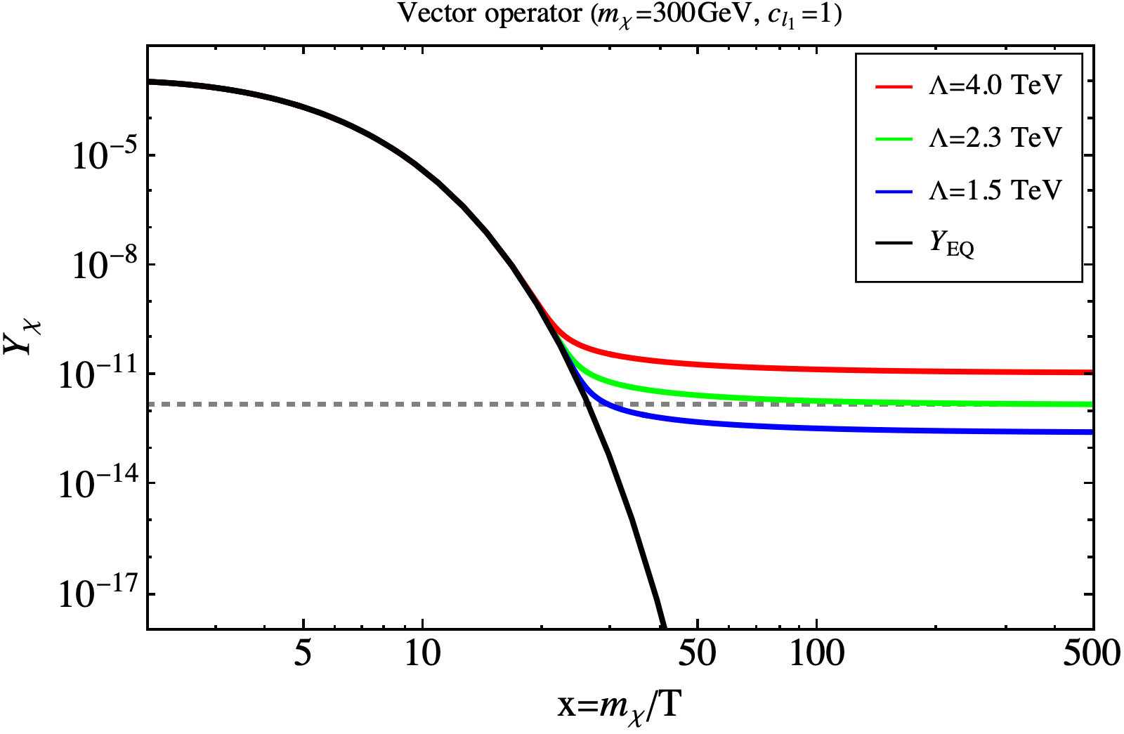
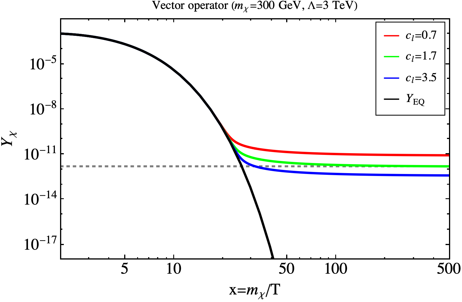
Figure 1: Left: Evolution of DM (Dirac) yield $Y_{\chi}$ with $x=m_{\chi}/T$ for operator $\mathcal{O}_{DL}^{6}$ (see Eq. (3)), for three different choices of the EFT scale $\Lambda=\{4.0,2.3,1.5\}$ TeV shown respectively in red, blue and green keeping $c_{\ell_{1}}=1$ and $m_{\chi}=$ 300 GeV fixed. Right: Same as left, but for a fixed $\Lambda=3$ TeV with three choices of $c_{\ell_{1}}=\{0.7,1.7,3.5\}$ shown in red, blue and green respectively. In both the plots the thick black curve shows the equilibrium DM yield ($Y_{\tt eq}$) and the grey dashed straight line indicates the yield that produces correct relic abundance (see Eq. (11)).

The relic abundance of DM after thermal freeze-out has an approximate analytical form

$$\Omega_{\tt DM}\,{\sf h}^{2}\simeq\frac{(1.04\times 10^{9}\,\text{GeV})x_{f}}{M_{\tt pl}\sqrt{g_{*}}(a+3b/x_{f})}\,,$$ (9)

with $\Omega_{\tt DM}=\rho_{\tt DM}/\rho_{c}$, where $\rho_{c},\rho_{\tt DM}$ denote the critical and DM densities respectively and $x_{f}=m_{\chi}/{T_{f}}$, with $T_{f}$ the freeze-out temperature when the DM decouples from thermal bath. In presence of all the operators with $c_{\ell_{i}}=1$, all the individual amplitudes add together to the total annihilation cross-section, with

$$\langle{\sigma v}\rangle_{\rm tot}\sim\Big{|}\sum_{\mathcal{O}_{i}}\mathcal{M}_{\mathcal{O}_{i}}\Big{|}^{2}\,,$$ (10)

where $\mathcal{M}_{\mathcal{O}_{i}}=\frac{c_{\ell_{i}}}{\Lambda^{2}}(\bar{\chi}\Gamma\chi)(\bar{\ell}\Gamma\ell);~{}\rm{with}~{}\Gamma=\{\gamma^{\mu},\gamma^{\mu}\gamma^{5}\}$ denote the matrix elements for DM pair annihilation to SM via respective operators as in Eq. (3). The relic density obtained from the model is then compared to the current Planck data Aghanim:2018eyx

$$\Omega_{\tt DM}{\sf h}^{2}=0.11933\pm 0.00091\,,$$ (11)

that finds relic density allowed parameter space of the model. In Fig. 1, we show the thermal freeze-out of the DM following Eq. (5) in $Y_{\chi}-x$ plane, for operator $\mathcal{O}_{DL}^{6}$ (see Eq. (3)) assuming a Dirac DM $\chi$. The equilibrium distribution $Y_{\tt eq}$ is shown by black thick line, where we choose $m_{\chi}=300$ GeV. Horizontal grey dashed line corresponds to $Y_{\chi}$ value for correct DM relic density following Eq. (11), which is approximately given by the condition $m_{\chi}Y_{\chi}\approx 0.44$ eV. In the left panel, we vary the EFT scale $\Lambda=\{4.0,2.3,1.5\}$ TeV, shown respectively by red, green and blue curves assuming $c_{\ell_{1}}=1$ and we see that the green curve with $\Lambda=2.3$ TeV provides the correct relic after freeze-out, whereas the case with larger (smaller) $\Lambda$, corresponding to the red (blue) curve in Fig. 1 provides over (under) abundance following the inverse dependence of relic density to annihilation cross-section as in Eq. (9). In the right panel of Fig. 1, we show the thermal freeze-out for three different choices of $c_{\ell_{1}}=\{0.7,1.7,3.5\}$ in red, green and blue respectively for a fixed $\Lambda=3$ TeV. Again, we see that the case with $c_{\ell_{1}}=1.7$ satisfy correct relic while the smaller (larger) $c_{\ell_{1}}$ provides over (under) abundance attributed to Eq. (9). The relic density allowed parameter space of the model can then be found in terms of $\{\Lambda,m_{\chi}\}$ assuming $c_{\ell_{i}}=1$. We use the numerical tool MicrOmegas Belanger:2010pz to compute relic density for the model for both Dirac and Majorana cases. The results, together with direct search constraints, will be discussed in the next section.

3.2 Direct detection

Direct DM search relies on the DM scattering with earthly detectors and observation of nuclear recoil to confirm the presence of DM interaction. Unfortunately no DM signal has been confirmed yet, resulting a strong bound on the DM-SM interaction cross-section, the latest from XENON1T XENON:2018voc . Leptophilic DM as defined, do not have a direct coupling to detector nucleus. But, it is possible to induce couplings to quarks via photon exchange at one loop level as in Fig. 2, where in the loop one may have any charged lepton to which the DM couples to. Instead of a nuclear recoil, it is also possible to knock off an electron from the atomic orbital of the detector material directly via the effective DM interaction with the lepton. However, as it has been shown in PhysRevD.80.083502 , the loop-induced DM-nucleon scattering always dominates over the DM-electron scattering cross-section, where the latter is suppressed by the momentum wave function. Therefore, we ignore the DM-electron scattering here and focus on the one loop DM-nucleus interaction via one loop. Now, following the most general 4-fermion interaction as in Eq. (4) Kopp:2009et , the one loop contribution to DM-nucleon interaction involves the following integration:

$$\int\frac{d^{4}q}{\left(4\pi\right)^{4}}\text{Tr}\Biggl{[}\Gamma_{\ell}\frac{\not{q}^{\prime}+m_{\ell}}{q^{{}^{\prime}2}-m_{\ell}^{2}}\gamma^{\mu}\frac{\not{q}+m_{\ell}}{q^{2}-m_{\ell}^{2}}\Biggr{]}\,,$$ (12)

where $q$ and $q^{\prime}=k-k^{\prime}+q$ denote the loop momentum, with $k,k^{\prime}$ as the momenta carried by the incoming and outgoing DM particles respectively. Note that, the loop contribution is non-zero only for vector and tensor lepton currents $\Gamma^{\mu}_{\ell}=\gamma^{\mu},\sigma^{\mu\nu}$. For scalar, pseudoscalar and axial-vector currents $\Gamma^{\mu}_{\ell}=1,\gamma_{5},\gamma^{\mu}\gamma_{5}$ this contribution in Eq. (12) identically vanish. Therefore, non-zero direct search contribution for leptophilic DM arises only for operators $\mathcal{O}_{DL}^{6},\mathcal{O}_{L}^{6}$. However, the contribution from $\mathcal{O}_{L}^{6}$ to the direct detection cross-section vanishes in the non-relativistic limit and $\mathcal{O}_{DL}^{6}$ doesn’t apply to Majorana DM. Therefore, direct detection constraints do not yield any bound on the parameter space for leptophilic (or hadrophilic) Majorana DM. Subsequently, we focus on the vector type interaction, namely $\mathcal{O}_{DL}^{6}=\frac{c_{\ell_{1}}}{\Lambda^{2}}(\bar{\chi}\gamma^{\mu}\chi)(\bar{\ell}\gamma_{\mu}\ell)$, and calculate the loop-induced matrix element relevant for nuclear recoil experiments.

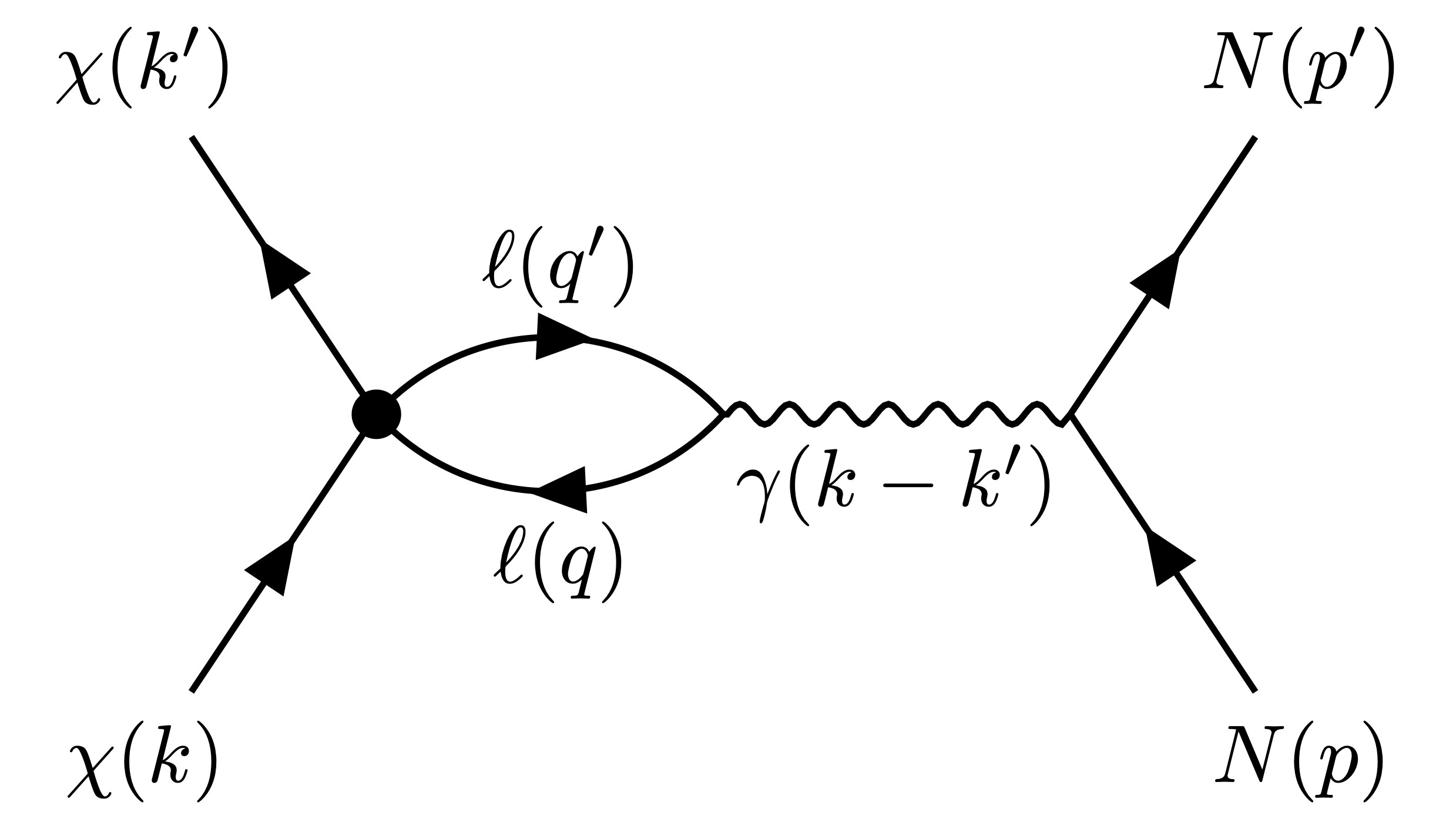
Figure 2: Loop-induced DM-nucleon direct detection mediated by a virtual photon. Here $q$ is the loop momentum, and $q^{\prime}=k-k^{\prime}+q$. The blob represents the effective nature of the vertex.

The matrix element for $\chi N\rightarrow\chi N$ scattering (where $N$ denotes detector nucleus) via one-loop interaction, modulo implicit sum over the light quark generations with charge $Q_{j}$ is thus given by:

$$\begin{split}&\mathcal{M}=L^{(1)}\Bigl{(}\overline{u}_{\chi}\,\gamma^{\mu}\,u_{\chi}\Bigr{)}\,\Bigl{\langle}N\Bigl{|}Q_{j}\,\Bigl{(}\overline{{\mathfrak{q}}}_{j}\gamma_{\mu}{\mathfrak{q}}_{j}\Bigr{)}\Bigr{|}N\Bigr{\rangle}=L^{(1)}\Bigl{(}\overline{u}_{\chi}\,\gamma^{\mu}\,u_{\chi}\Bigr{)}Z\,F\left(q\right)\,\Bigl{(}\overline{u}_{N}\,\gamma_{\mu}\,u_{N}\Bigr{)}\,,\end{split}$$ (13)

where $F\left(q\right)$ denotes the nuclear form factor, $Z$ denotes the Atomic number of the nucleus and the loop factor $L^{(1)}$ is given by

$$L^{(1)}=\frac{2\alpha_{\text{em}}}{\pi}\frac{c_{\ell_{1}}}{\Lambda^{2}}\int_{0}^{1}\,dx\,x\left(1-x\right)\ln\Biggl{[}\frac{-x\left(1-x\right)\mathcal{Q}^{2}+m_{\ell}^{2}}{\mu^{2}}\Biggr{]}\,.$$ (14)

$\mathcal{Q}$ in the above expression momentum transfer ($\mathcal{Q}=k-k^{\prime}$) in the process and $\mu$ is the renormalization scale. For $m_{\ell}\gg\left|\bf{\mathcal{Q}}\right|$ one may neglect the momentum transfer and obtain

$$L_{LL}^{(1)}\approx\frac{2\alpha_{\text{em}}}{\pi}\frac{c_{\ell_{1}}}{\Lambda^{2}}\underbrace{\int_{0}^{1}\,dx\,x\left(1-x\right)\ln\Biggl{[}\frac{m_{\ell}^{2}}{\mu^{2}}\Biggr{]}}_{=\frac{1}{6}\ln\Biggl{[}\frac{m_{\ell}^{2}}{\mu^{2}}\Biggr{]}}=\frac{\alpha_{\text{em}}}{3\pi}\frac{c_{\ell_{1}}}{\Lambda^{2}}\ln\Biggl{[}\frac{m_{\ell}^{2}}{\mu^{2}}\Biggr{]}+\mathcal{O}\Bigl{(}\left|\bf{\mathcal{Q}}\right|/m_{\ell}\Bigr{)}\,,$$ (15)

where $LL$ stands for the “leading log” contribution, neglecting the remaining logarithmic dependence on momentum transfer. With the leading log approximation the matrix element takes the form

$$\begin{split}&\mathcal{M}=\Biggl{(}\frac{\alpha_{\text{em}}}{3\pi}\frac{c_{\ell_{1}}}{\Lambda^{2}}\log\Biggl{[}\frac{m_{\ell}^{2}}{\mu^{2}}\Biggr{]}ZF\left(q\right)\Biggr{)}\Bigl{(}\overline{u}_{\chi}\,\gamma^{\mu}\,u_{\chi}\Bigr{)}\Bigl{(}\overline{u}_{N}\,\gamma_{\mu}\,u_{N}\Bigr{)}.\end{split}$$ (16)

For a single operator it is possible to compute the direct search cross-section analytically as illustrated Kopp:2009et . However, since we are considering all operators together, it is difficult to obtain an analytical expression for the loop-induced direct detection cross-section. More importantly, the Wilson coefficients ($c_{\ell_{i}}$) can vary substantially from the typical energies for obtaining DM relic density (where they are defined) to the typical energies of DM direct search experiments ($\sim$ GeV). We use the runDM DEramo:2016gos package to obtain couplings at the energy scale of direct detection $\sim 2~{}\rm GeV$ starting from energy scale of $\sim$ TeV where the Wilson coefficients are assumed to be $c_{\ell_{i}}=1$. The renormalization group evolution (RGE) typically introduces mixing between different DM-SM interactions, affecting the size of couplings, and even inducing new couplings which do not appear in a naive comparison. The relic density calculation however remains unaffected with or without the running.

Note that the matrix element in Eq. (16) depend on the renormalization scale $\mu$. To extract physical quantities that does not depend on $\mu$, we need to define the renormalization condition. In our case this condition is that at scale $\Lambda\sim 1$ TeV, the coefficient ($c_{q_{1}}^{({\mathfrak{q}}_{j})}$) of the effective DM-quark operator $(\bar{\chi}\gamma^{\mu}\chi)(\bar{{\mathfrak{q}}}_{j}\gamma_{\mu}{\mathfrak{q}}_{j})$ is zero. As an illustrative example with only one generation of lepton, in the leading-log approximation (following Eq. (16)), at the $\overline{\text{MS}}$ scale $\mu$, the coefficient $c_{q_{1}}^{({\mathfrak{q}}_{j})}$ reads

$$c_{q_{1}}^{({\mathfrak{q}}_{j})}(\mu)\approx Q_{j}\frac{\alpha_{\rm em}}{3\pi}\frac{c_{\ell_{1}}}{\Lambda^{2}}\ln\bigg{(}\frac{m_{\ell}^{2}}{\mu^{2}}\bigg{)}\,.$$ (17)

Therefore, our renormalization condition reads

$$c_{q_{1}}^{({\mathfrak{q}}_{j})}(\Lambda)\approx Q_{j}\frac{\alpha_{\rm em}}{3\pi}\frac{c_{\ell_{1}}}{\Lambda^{2}}\ln\bigg{(}\frac{m_{\ell}^{2}}{\Lambda^{2}}\bigg{)}=0\,,$$ (18)

where we set $\mu\equiv\Lambda$ Kopp:2009et . Using Eq. (18), it is easy to infer the coefficient at any energy scale $\Lambda_{f}$ ($\leq\Lambda$) as

$$c_{q_{1}}^{({\mathfrak{q}}_{j})}(\Lambda_{f})\approx Q_{j}\frac{\alpha_{\rm em}}{3\pi}\frac{c_{\ell_{1}}}{\Lambda^{2}}\ln\bigg{(}\frac{\Lambda^{2}}{\Lambda_{f}^{2}}\bigg{)}\ .$$ (19)

Relevant Scales	$c_{q_{1}}^{(u)}$	$c_{q_{1}}^{(d)}$	$c_{q_{1}}^{(c)}$	$c_{q_{1}}^{(s)}$	$c_{q_{1}}^{(b)}$	$c_{\ell_{1}}^{(e)}$	$c_{\ell_{1}}^{(\mu)}$	$c_{\ell_{1}}^{(\tau)}$
$\Lambda=3$ TeV	0	0	0	0	0	1	1	1
$\Lambda_{\rm NR}=2$ GeV	0.024	-0.012	0.024	-0.012	-0.012	0.965	0.965	0.965

Table 1: Running of the coupling coefficients $c_{q_{1}}^{({\mathfrak{q}})}$, and $c_{\ell_{1}}^{(\ell)}$ of the operators ${\cal O}_{DQ}^{6}$ and ${\cal O}_{DL}^{6}$ respectively (see Eq. (3)) using runDM package, from an initial scale $\Lambda=3$ TeV to the non-relativistic scale $\Lambda_{\rm NR}=2$ GeV relevant for DM-nucleon scattering. For Leptophilic case, only non-zero coefficient of the operator ${\cal O}_{DL}^{6}$ is assumed with $c_{\ell_{1}}^{(\ell)}=1$, at the scale $\Lambda$. Note that this is only relevant for Dirac DM, as the vector DM current is zero for the Majorana case.

Notice in Eq. (19), that $c_{q_{1}}^{({\mathfrak{q}}_{j})}$ is zero at the scale $\Lambda_{f}=\Lambda$, as per renormalization condition. The DM-nucleon cross section at direct detection scale $\Lambda_{\text{NR}}$, is then given by

$$\sigma_{\rm SI}\approx\frac{\mu_{p}^{2}c_{\ell_{1}}^{2}}{9\pi A^{2}}\Biggl{(}\frac{\alpha_{\text{em}}Z}{\pi\Lambda^{2}}\Biggr{)}^{2}\Biggl{[}\ln\Biggl{(}\frac{\Lambda^{2}}{\Lambda_{\text{NR}}^{2}}\Biggr{)}\Biggr{]}^{2}\,,$$ (20)

where we have ignored the term proportional to DM velocity $v\sim 10^{-6}$, used $F(q)=1$ for brevity and $\mu_{p}=m_{p}\,m_{\chi}/\left(m_{p}+m_{\chi}\right)$ as the reduced mass of the DM-nucleon system. Its worth reminding that in deriving Eq. (20), we have assumed the presence of only the vector operator $\mathcal{O}_{DL}^{6}=\frac{c_{\ell_{1}}}{\Lambda^{2}}(\bar{\chi}\gamma^{\mu}\chi)(\bar{\ell}\gamma_{\mu}\ell)$ at the effective scale $\Lambda$. The running of the couplings to a lower scale ($\Lambda_{\rm{NR}}$) generates the DM-quark interaction via operator mixing, thereby producing the spin-independent direct detection cross-section as in Eq. (20). In Table 1, we show the values of the running coupling coefficients $c_{q_{1}}^{({\mathfrak{q}})}$, and $c_{\ell_{1}}^{(\ell)}$ at direct search experiment scale $\Lambda_{\text{NR}}=2$ GeV evaluated using runDM package, while the input values are assumed at NP scale $\Lambda=3$ TeV. Using them, together with $m_{\chi}=500$ GeV, we find $\sigma_{\rm SI}\approx 3\times 10^{-47}~{}\text{cm}^{2}$, close to the sensitivity of existing direct search cross-section. It is clear, that the loop-induced WIMP-nucleon spin-independent scattering cross-section can provide a very strong bound on the leptophilic DM parameter space, which will be shown together with the relic density allowed parameter space in Subsection. 3.4.

3.3 Indirect detection

Although DM occasionally annihilate after thermal-freeze-out, it can still occur in regions with very large DM density, for example, at the centre of galaxies. The annihilations produce a bunch of SM particles in pair of various kinds, such as:

$$\chi+\bar{\chi}\rightarrow f\bar{f},~{}\gamma\gamma,...~{}~{}f:~{}\text{SM ~{}fermions};$$

where the presence of anti-particle ($\bar{f}$) and photons in particular, play crucial role in elucidating the presence of DM, if an excess is found. Various satellite and ground based telescopes (like the Fermi Large Area Telescope (FermiLAT) Fermi-LAT:2016afa or Cherenkov Telescope Array (CTA) CTAConsortium:2012fwj ) have searched for excess in anti-particle or photons beyond astrophysical processes which may arise from the DM annihilation. For example, the production rate ($\Gamma$) of SM particles from DM annihilation is crucially dependent on parameters like DM density ($\rho_{\tt DM}$) and strength of annihilation cross-section $(\sigma v)$ Cirelli:2010xx ; Slatyer:2017sev ; Hooper:2018kfv

$$\Gamma\sim\int_{V}\left(\frac{\rho^{2}_{\tt DM}}{m_{\chi}^{2}}\right)dV\times(\sigma v)(N_{\text{SM}});$$ (21)

where $N_{\text{SM}}$ represents number of SM particles per annihilation event. Note that annihilation cross-section present in the equation above is also crucial to produce thermal freeze-out for WIMP like DM to produce correct relic density. In context of the effective leptophilic DM operators that we are concerned, we can therefore calculate annihilation cross-section to produce current indirect search observation and relate to the annihilation cross-section to produce correct relic density and thus produce a bound on the model. We further note that significant constraint can only be obtained for leptophilic Dirac DM as Majorana DM would produce velocity dependent annihilation cross-section, which results in a suppressed annihilation rate, and hence does not provide any reasonable bound from indirect detection. A detailed analysis of indirect detection bound on the DM parameter space is beyond the scope of this paper. We simply calculate the thermal averaged DM pair annihilation cross-section into different SM leptonic final states as shown in table 2, and project the bound from the non-observation of gamma-ray signals from DM annihilation in dwarf satellite galaxies MAGIC:2016xys . In the absence of any boost factor viz., Sommerfeld enhancement Feng:2010zp , the bounds from indirect search turns out to be much milder than that due to direct detection, and constraints the relic density allowed parameter space for the DM only at very low $m_{\chi}$.

$\langle\sigma v\rangle_{\chi\bar{\chi}\rightarrow e^{+}e^{-}}$ $({\rm cm}^{3}/{\rm s})$	$\langle\sigma v\rangle_{\chi\bar{\chi}\rightarrow\mu^{+}\mu^{-}}$ $({\rm cm}^{3}/{\rm s})$	$\langle\sigma v\rangle_{\chi\bar{\chi}\rightarrow\tau^{+}\tau^{-}}$ $({\rm cm}^{3}/{\rm s})$
$7.5\times 10^{-27}$	$7.5\times 10^{-27}$	$7.5\times 10^{-27}$

Table 2: Velocity averaged annihilation cross-section $\langle\sigma v\rangle$ (s-wave) of dominating channels for the relic density satisfying points. We have chosen illustrative values $c_{\ell_{i}}=1$ (Dirac DM). The annihilation to quark final states are negligibly small in comparison to the leptonic final states. Note that the annihilation to neutrino final states are identically zero due to interference effects (e.g., see Eq. (34)).

3.4 Viable parameter space

  

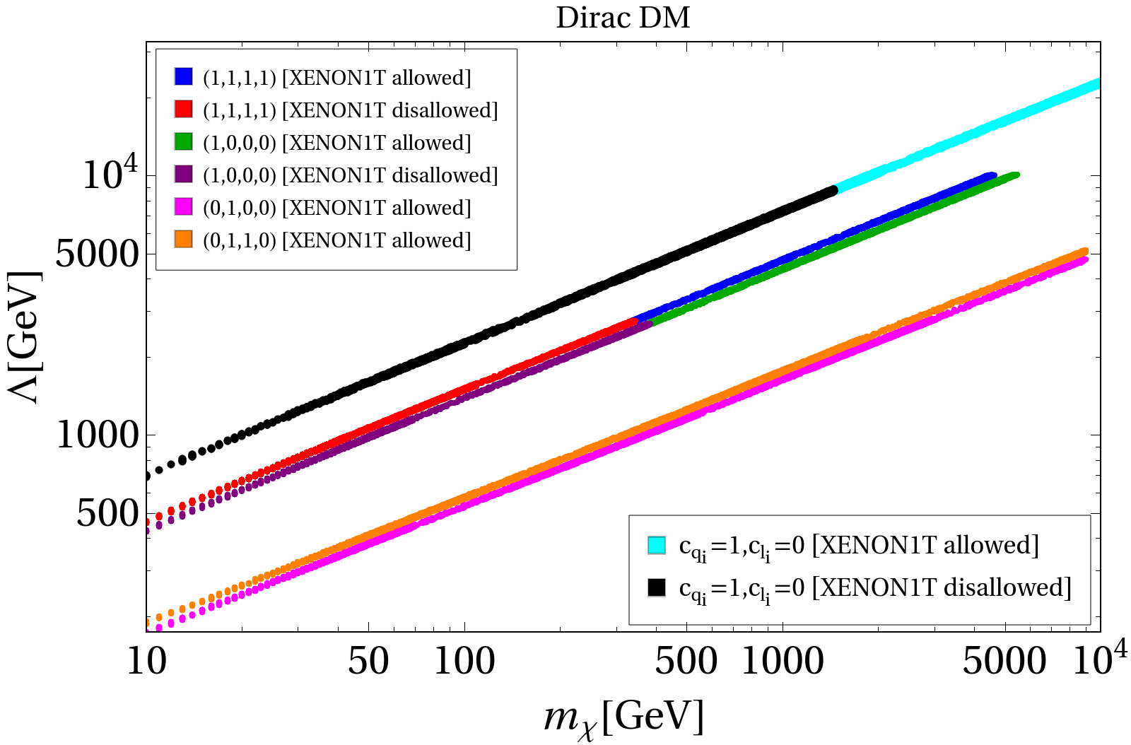
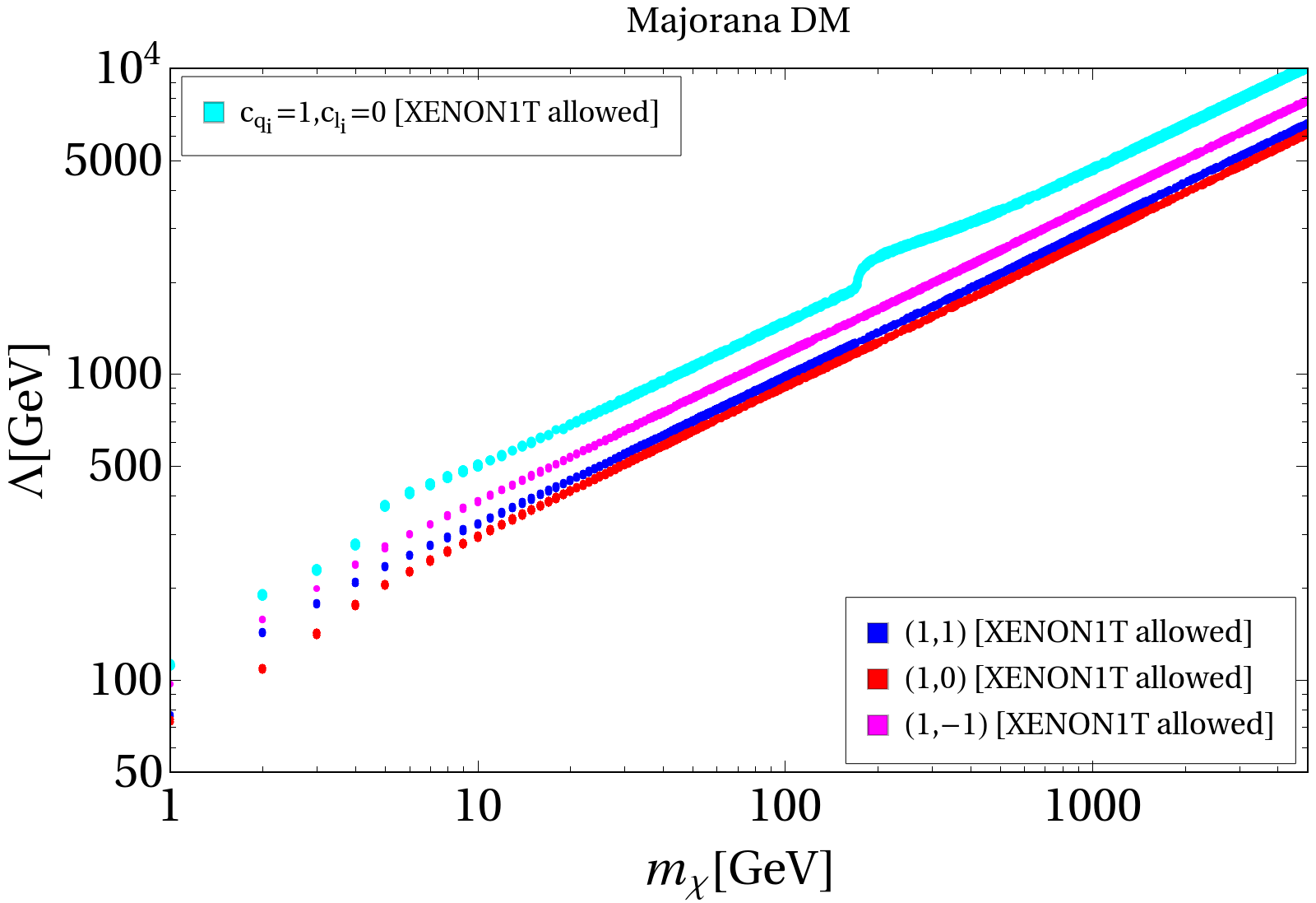
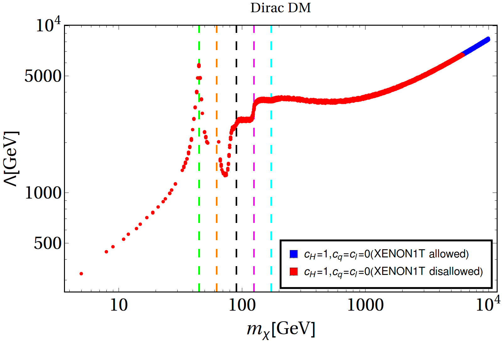
Figure 3: Relic density and direct search (XENON1T) allowed parameter space for hadrophilic ($c_{q_{i}}=1,c_{\ell_{i}}=0$), and leptophilic ($c_{q_{i}}=0,c_{\ell_{i}}=1$) cases in the top panel and Higgs portal case ($c_{H_{i}}=1,c_{\ell_{i}}=c_{q_{i}}=0$) in the bottom panel. Top Left (right) figure describes Dirac (Majorana) DM. The coupling values $(c_{\ell_{1}},c_{\ell_{2}},c_{\ell_{3}},c_{\ell_{4}})$ is denoted as an ordered set for Dirac DM and $(c_{\ell_{2}},c_{\ell_{3}})$ for Majorana DM. XENON1T allowed region and disallowed regions are marked in different colours (see figure inset and text for details); for example, in hadrophilic Dirac DM case (top left), XENON1T allowed region is shown in cyan, while the disallowed region is shown in black. Note, there is no spin-independent direct detection bound on Majorana DM.

After discussing the major constraints on DM model coming from relic density, direct and indirect search experiments, we summarise here the available DM parameter space for leptophilic DM operators from all of these constraints, in terms of $m_{\chi}-\Lambda$. In Fig. 3 we show the Planck observed relic density allowed parameter space for Dirac (top left) and Majorana (top right) DM in $\Lambda-m_{\chi}$ plane by considering all relevant operators together for both hadrophilic ($c_{\ell_{i}}=0,c_{q_{i}}=1$) and leptophilic ($c_{\ell_{i}}=1,c_{q_{i}}=0$) cases. We vary the two free parameters of the theory, namely the cut-off scale $\Lambda$ and the DM mass $m_{\chi}$, in the following range

$$\Lambda:\{1-10^{4}\}~{}\text{GeV};~{}m_{\chi}:\{1-10^{4}\}~{}\text{GeV}$$

while considering $\Lambda\gtrsim m_{\chi}/2\pi$ in order to make sure that the effective theory description remains valid. First of all, notice that in all plots, with the increase in DM mass, $\Lambda$ also rises to satisfy the relic abundance, following that the relic density of thermal WIMP goes as $\Omega_{\chi}h^{2}\sim 1/\langle\sigma v\rangle\sim\Lambda^{4}/m_{\chi}^{2}$. XENON1T allowed region and disallowed regions are marked in different colours.

In the top left plot of Fig. 3, for hadrophilic case, the relic density allowed region is significantly ruled out from spin-independent direct detection bound upto $m_{\chi}\lesssim 6.4~{}\rm TeV$ for $\Lambda\lesssim 18~{}\rm TeV$ (shown by black points) making it difficult for collider probe. In the same plot, we also show the leptophilic cases where coupling values $(c_{\ell_{1}},c_{\ell_{2}},c_{\ell_{3}},c_{\ell_{4}})$ is denoted as an ordered set for Dirac DM. Amongst different possibilities considered, we see that vector coupling plays a crucial role as those cases with $c_{\ell_{1}}=1$ almost overlap and segregates from those with $c_{\ell_{1}}=0$. As explained earlier in Sec. 3.2, the loop-induced direct search plays an important role as this rules out leptophilic DM mass $m_{\chi}$ and $\Lambda$ significantly. For example, (1,1,1,1) case is ruled out upto $(m_{\chi},\Lambda)\sim$(345, 2780) GeV, and (1,0,0,0) case is ruled out upto $(m_{\chi},\Lambda)\sim$(380, 2700) GeV. Other choices of model parameters, such as (1,1,0,0), (1,1,1,0) etc. are very close to the (1,0,0,0) case and hence we did not show them here. Note that for the cases with $c_{\ell_{1}}=0$, the spin-independent direct search cross-section vanishes, and there is no bound on $\Lambda-m_{\chi}$ parameter space from direct detection. Also notice that for the same $m_{\chi}$, the leptophilic cases requires a lower $\Lambda$ than the hadrophilic case to satisfy relic abundance. This stems from larger annihilation cross-section due to the color factor to quark final states, which therefore requires a comparatively larger $\Lambda$ to tame down the annihilation cross-section to satisfy the DM relic.

The same exercise is done for Majorana DM in the top right panel of Fig. 3 for both leptophilic (red, blue, and magenta) and hadrophilic (cyan) case. Couplings $(c_{\ell_{2}},c_{\ell_{3}})$ are used as an ordered pair for defining Majorana DM models. We again see here, that the hadrophilic case requires larger $\Lambda$ than the leptophilic cases following the same line of arguments as before. Here one should notice the presence of two prominent bumps corresponding to the opening of $b\bar{b}$ and $t\bar{t}$ final states for the hadrophilic case. For Majorana DM, there is no significant direct detection bound because of the absence of DM vector current, and due to the fact that the contribution of ${\cal O}_{L}^{6}$ (see Eq. (3)) to the direct detection cross-section vanishes in the non-relativistic limit. This makes all of the relic density allowed parameter space available starting from DM mass as low as 1 GeV with $\Lambda\sim 10~{}\rm GeV$.

We have also shown the allowed parameter space corresponding to the Higgs portal operators with $(c_{H_{i}}=1,c_{q_{i}}=c_{\ell_{i}}=0)$ case for comparison in the bottom panel of Fig. 3. The vertical black dashed lines correspond to (from left to right) resonances due to $Z$ and Higgs boson, opening of $Z$, Higgs and top quark final states respectively. Here we see both relic density and direct detection bounds are satisfied for $m_{\chi}\gtrsim 6.2~{}\rm TeV$ and $\Lambda\gtrsim 7~{}\rm TeV$, again making this model difficult to probe in ongoing collider experiment. We carry out the analysis of viable parameter space with negative Wilson coefficients in Appendix B.

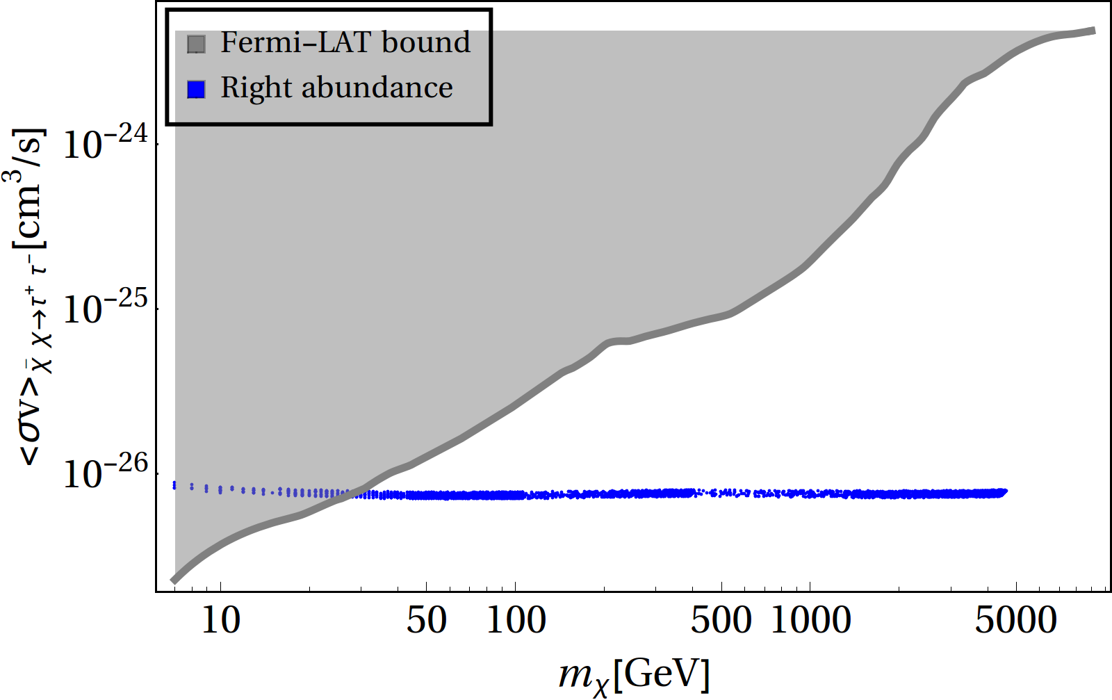
Figure 4: Indirect detection bound on Dirac DM annihilation cross-section. The gray region is excluded from the combined data analysis of MAGIC cherenkov telescopes and Fermi large area telescope (FermiLAT) that searched for the gamma-ray signals from DM annihilation MAGIC:2016xys . The blue points represent thermally averaged annihilation cross-section ($\langle\sigma v\rangle)$ for DM annihilating into $\tau^{+}\tau^{-}$ pair. As can be seen from the figure, this bound rules out DM having mass below $30$ GeV.

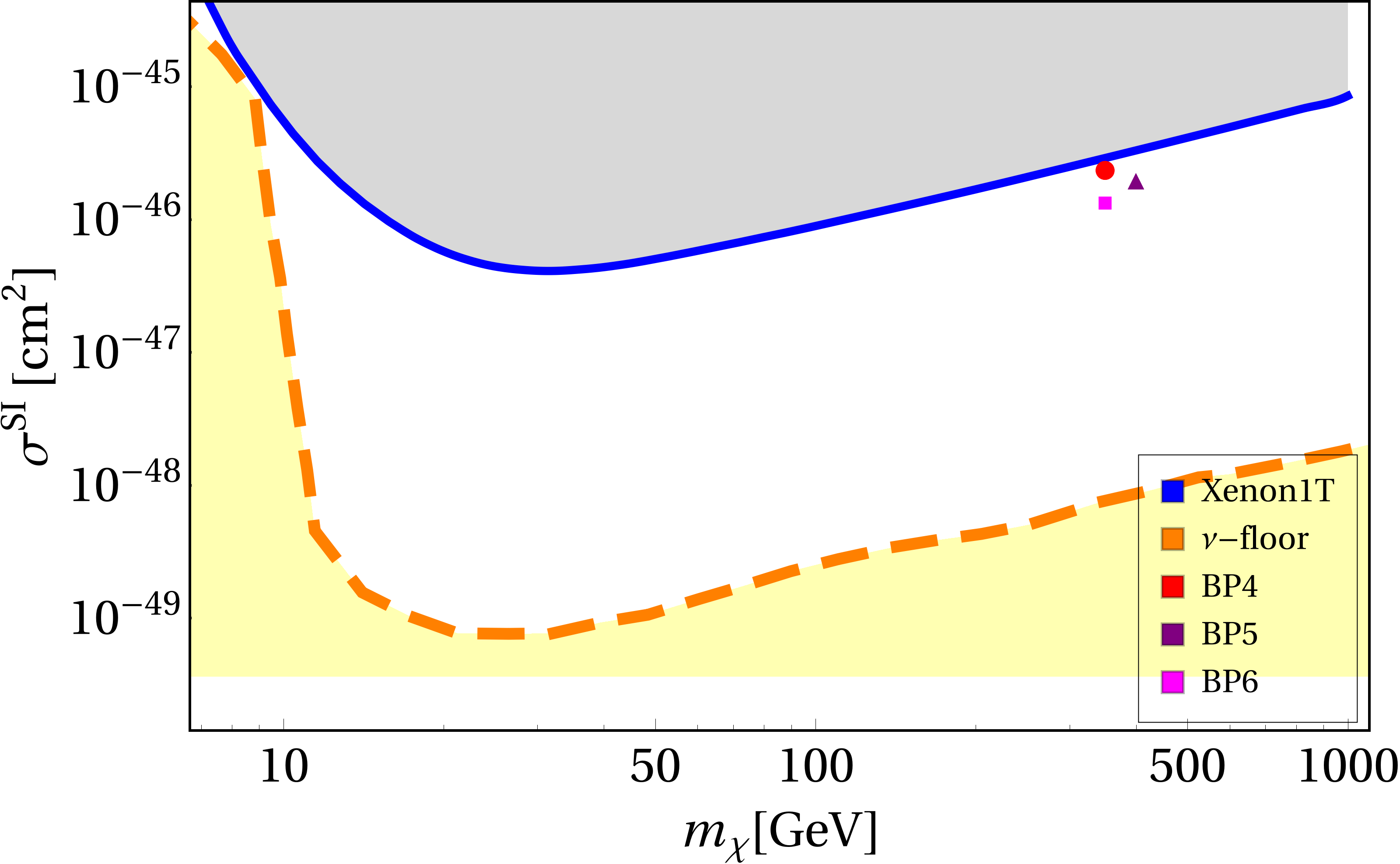
Figure 5: Benchmark points (BP4 in red, BP5 in purple and BP6 in magenta: see table 3) for Dirac DM confronted with XENON1T bound shown by gray excluded region in $m_{\chi}$ (in GeV) versus the spin-independent direct detection cross-section $\sigma_{\rm SI}$ (in cm²) plane. The Yellow region at the bottom corresponds to neutrino floor. Note that Majorana DM do not face any direct search constraints in leptophilic case as considered.

Let us now turn to indirect search bounds. The constraint on thermally-averaged cross-section for $\tau^{+}\tau^{-}$ final state in our model yields a bound on Dirac DM mass, namely $m_{\chi}\lesssim 30$ GeV (Fig. 4). This bound is much less stringent than the bound from direct detection (as in Fig. 3). In further analysis for collider search, we therefore address benchmark points where DM constraints are coming mainly from relic density and direct search. A few such benchmark points are tabulated in table 3 where we specify the DM mass ($m_{\chi}$), corresponding NP scale ($\Lambda$) and Wilson coefficients as input model parameter in an ordered set $(c_{\ell_{1}},c_{\ell_{2}},c_{\ell_{3}},c_{\ell_{4}})$ for Dirac case and $(c_{\ell_{2}},c_{\ell_{3}})$ for Majorana DM cases. The benchmark points for Dirac DM are also represented in the spin-independent direct detection cross-section ($\sigma_{\rm SI}$ (in cm²) plane) versus DM mass plane in Fig. 5 with XENON1T bound. As Majorana DM do not face any bound from direct search, corresponding benchmark points can’t be shown in this plane.

DM scenario	Benchmark Points	Model	$m_{\chi}$ (GeV)	$\Lambda$ (GeV)
	BP1	$(1,1)$	70	816
Majorana	BP2	$(1,1)$	112	1025
	BP3	$(1,-1)$	70	990
	BP4	$(1,1,1,1)$	350	2800
Dirac	BP5	$(1,1,1,1)$	400	3000
	BP6	$(1,1,-1,-1)$	350	3300

Table 3: Benchmarks points satisfying DM relic density and direct detection constraints for Majorana (BP1, BP2, BP3) and Dirac (BP4, BP5, BP6) DM scenario considering all leptophilic operators together. Different choices for the Wilson coefficients are denoted as different models and represented as an ordered set of allowed $\{c_{\ell_{i}}\}$. For example, $(1,1,-1,-1)$ in BP6 refers to the choice $(c_{\ell_{1}}=1,c_{\ell_{2}}=1,c_{\ell_{3}}=-1,c_{\ell_{4}}=-1)$, whereas $(1,-1)$ in BP3 denotes $(c_{\ell_{2}}=1,c_{\ell_{3}}=-1)$.

Before closing this section, we would like to mention that the recent result from PandaX-4T PandaX-4T:2021bab puts a stringent bound on the spin-independent DM-nucleon cross-section, for example, $3.3\times 10^{-47}~{}\text{cm}^{2}(90\%$ C.L.) for $\hbox{m}_{\chi}\sim$ 30 GeV. Satisfying this exclusion limit follows a similar exercise as above and requires an even larger mass ($m_{\chi}$) and effective scale ($\Lambda$) for Dirac DM (when $c_{\ell_{1}}\neq 0$), like $\{m_{\chi},\Lambda\}:\{430,3150\}~{}\rm GeV$. Note that this can still be probed at a 1 TeV lepton collider. However, for further analysis we content ourselves with the already published limit from XENON1T data XENON:2018voc .

4 Collider search prospects of Leptophilic DM

It is obvious that DM operators that connects to SM leptons have very suppressed production (via loop) at the currently running LHC and given the SM background contribution, it is difficult to find them at LHC.

  

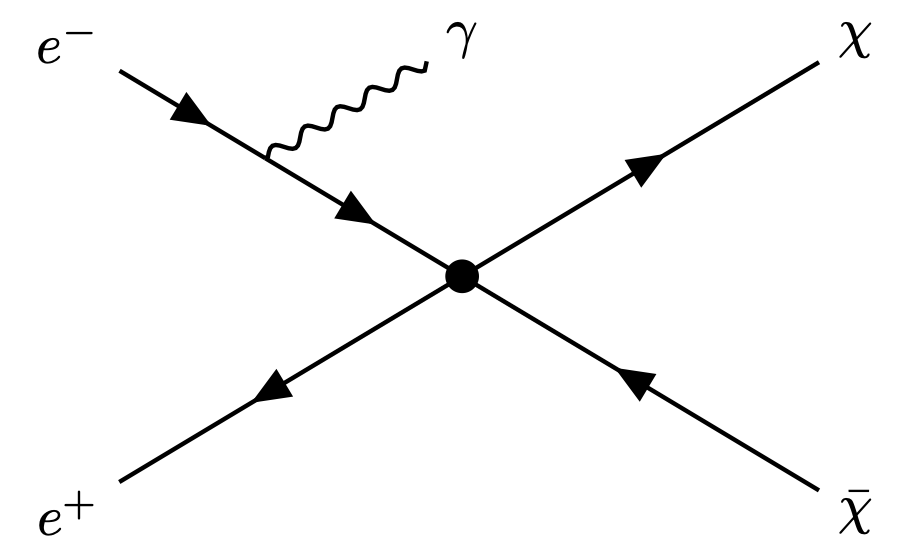
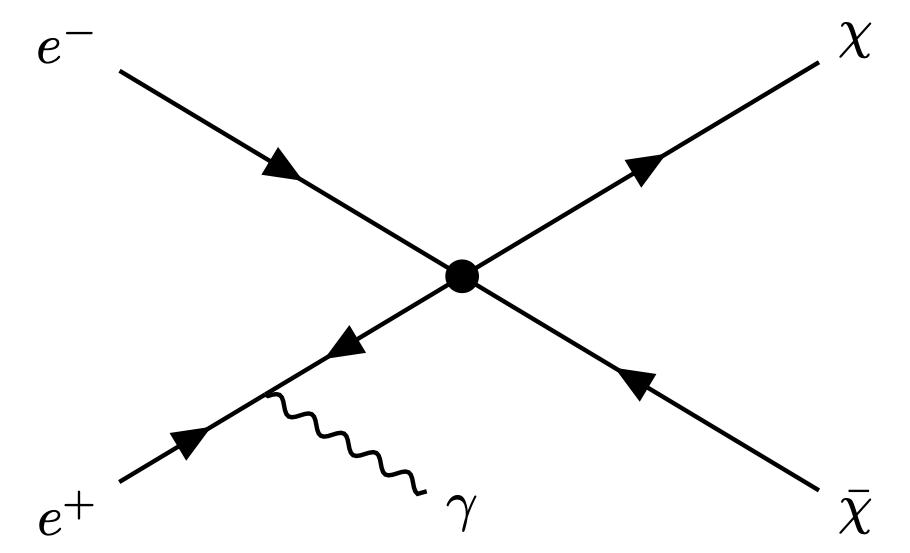
Figure 6: Mono-photon with missing energy $\gamma+\not{E_{T}}$ signature at the collider where the photon is irradiated from the initial state charged leptons. The blob represents the effective nature of the vertex.

On the other hand, such operators can be probed at $e^{+}e^{-}$ machine. The main production of DM occurs via the contact interaction dictated by the EFT operators. However, DM being invisible at the detector a pair production of DM would not produce a signal at the detector, so one needs to rely upon one or more initial state radiation (ISR) photon. Therefore, the signal in such a case is predominantly given by

$$e^{+}e^{-}\rightarrow\chi\bar{\chi}+\gamma\rightarrow\text{ME}+\gamma\,;$$ (22)

where ME refers to missing energy with monophoton. The Feynman graph is shown in Fig. 6. Note that higher multiplicity of radiated photon will diminish the cross-section of the process further. Therefore, mono-photon events with missing energy is a vanilla EFT signature of DM production at colliders that have been extensively studied in the literature in context with both hadron and lepton colliders.

As has been emphasized already, in a hadron collider, since the partonic CM frame is not the same as the hadronic CM frame, it is rather inconsistent to apply effective theory. The leptonic collider, on the other hand, provides a simple kinematics where a higher NP scale ($\Lambda$) compared to the known CM energy ($\sqrt{s}$), with $\Lambda>\sqrt{s}$ makes the EFT limit validated. As we have seen from the previous section, for a hadrophilic Dirac DM, the spin-independent direct search limit on the relic density allowed parameter space becomes so severe that it only allows DM as heavy as about $m_{\chi}\sim$ 6 TeV with the NP scale as large as $\Lambda\sim$ 18 TeV, that lies almost out of LHC sensitivities. For a leptophilic Dirac DM, on the other hand, it is possible to bring down the allowed DM mass to about 345 GeV with $\Lambda\sim 2.8~{}\rm TeV$. Such a DM can not certainly be pair-produced at a lepton collider with $\sqrt{s}=500~{}\rm GeV$, but can be probed with CM energy of 1 TeV. For leptophilic Majorana DM since all of its relic density satisfying parameter space is also allowed by direct search limits, this scenario is testable at a lepton collider with CM energy of 500 GeV or even below. In the following we perform event-level collider simulation for both Dirac and Majorana DM at those select benchmark points mentioned in Table 3.

It is worth mentioning here that constraints on leptophilic DM from mono-photon searches at LEP have been analyzed in Fox:2011fx using effective interactions and investigated with experimental data from DELPHI DELPHI:2003dlq ; DELPHI:2008uka . This results in a bound on the effective DM-electron coupling scale, $\Lambda:250-500$ GeV for DM mass $m_{\chi}\lesssim 80$ GeV, depending on the operator structure. The most stringent bound on $\Lambda$ arises from vector current (i.e., $O^{6}_{DL}$ in our case) which disallows $\Lambda<500$ GeV at 90% C.L. for $m_{\chi}\lesssim 60$ GeV. For DM mass $m_{\chi}\gtrsim 100$ GeV, LEP is completely insensitive for kinematic reasons. On the other hand, LHC bound on leptophilic DM has been discussed in Bell:2014tta , where the DM communicates with the SM via leptophilic $Z^{\prime}$ and the interaction with quarks (partons) take place via 1-loop. However, the bounds are model-dependent, and analyzed for $4\ell+\not{E_{T}}$ final states, taking each lepton flavour in turn. Hence, this is not directly applicable for our framework. In Table 3, all the benchmark points are well above the LEP exclusion limit.

4.1 DM Production cross-section and beam polarization

The central point of the collider analysis depends on the DM production cross-section at $e^{+}e^{-}$ collider. Here we elaborate on that. Since the electroweak part of the SM is chiral, appropriate beam polarization may be helpful to reduce SM backgrounds and increase NP signal, so we focus on polarized beams. The general expression for differential cross-section of the process $e^{+}e^{-}\rightarrow\chi\bar{\chi}$ with partial beam polarization ($-1<P_{e^{\pm}}<1$) is given by Fujii:2018mli ; Bambade:2019fyw

$$\begin{split}\frac{d\sigma(P_{e^{-}},P_{e^{+}})}{d\Omega}&=\frac{1}{4}\Biggl{\{}\Bigl{(}1+P_{e^{-}}\Bigr{)}\Bigl{(}1+P_{e^{+}}\Bigr{)}\bigg{(}\frac{d\sigma}{d\Omega}\bigg{)}_{\rm RR}+\Bigl{(}1-P_{e^{-}}\Bigr{)}\Bigl{(}1-P_{e^{+}}\Bigr{)}\bigg{(}\frac{d\sigma}{d\Omega}\bigg{)}_{\rm LL}\\ &+\Bigl{(}1+P_{e^{-}}\Bigr{)}\Bigl{(}1-P_{e^{+}}\Bigr{)}\bigg{(}\frac{d\sigma}{d\Omega}\bigg{)}_{\rm RL}+\Bigl{(}1-P_{e^{-}}\Bigr{)}\Bigl{(}1+P_{e^{+}}\Bigr{)}\bigg{(}\frac{d\sigma}{d\Omega}\bigg{)}_{\rm LR}\Biggr{\}}\,,\end{split}$$ (23)

where $\sigma_{ij}$ with $i,j\in L,R$ is the cross section for a given process with completely polarized beams of the four possible orientations. The final state of our interest are fermion pairs and the operators that mediate the DM-SM interactions are either vector or axial-vector operators. Hence, spin conservation indicates that the total spin of initial state should either be $\pm 1$, indicating that $\sigma_{\rm RR}=\sigma_{\rm LL}=0$ always, reducing the cross-section to the form:

$$\frac{d\sigma(P_{e^{-}},P_{e^{+}})}{d\Omega} =\frac{(1+P_{e^{-}})(1-P_{e^{+}})}{4}\bigg{(}\frac{d\sigma}{d\Omega}\bigg{)}_{\rm RL}$$

$$+\frac{(1-P_{e^{-}})(1+P_{e^{+}})}{4}\bigg{(}\frac{d\sigma}{d\Omega}\bigg{)}_{\rm LR}$$

where, for Dirac DM,

$$\bigg{(}\frac{d\sigma}{d\Omega}\bigg{)}^{\tt dirac}_{\rm RL} =\frac{s\sqrt{1-\beta_{\chi}^{2}}}{32\pi^{2}\Lambda^{4}}\bigg{[}\Big{\{}\ (1+\beta^{2}_{\chi})(c_{\ell_{1}}+c_{\ell_{4}})^{2}+(1-\beta^{2}_{\chi})(c_{\ell_{2}}+c_{\ell_{3}})^{2}\Big{\}}+4\sqrt{1-\beta^{2}_{\chi}}$$

$$\quad\Big{\{}(c_{\ell_{1}}+c_{\ell_{4}})(c_{\ell_{2}}+c_{\ell_{3}})\Big{\}}\cos\theta+(1-\beta^{2}_{\chi})\Big{\{}(c_{\ell_{1}}+c_{\ell_{4}})^{2}+(c_{\ell_{2}}+c_{\ell_{3}})^{2}\Big{\}}\cos^{2}\theta\bigg{]}\ ,$$ (25)

$$\bigg{(}\frac{d\sigma}{d\Omega}\bigg{)}^{\tt dirac}_{\rm LR} =\frac{s\sqrt{1-\beta_{\chi}^{2}}}{32\pi^{2}\Lambda^{4}}\bigg{[}\Big{\{}\ (1+\beta^{2}_{\chi})(c_{\ell_{1}}-c_{\ell_{4}})^{2}+(1-\beta^{2}_{\chi})(c_{\ell_{2}}-c_{\ell_{3}})^{2}\Big{\}}+4\sqrt{1-\beta^{2}_{\chi}}$$

$$\quad\Big{\{}(c_{\ell_{4}}-c_{\ell_{1}})(c_{\ell_{2}}-c_{\ell_{3}})\Big{\}}\cos\theta+(1-\beta^{2}_{\chi})\Big{\{}(c_{\ell_{1}}-c_{\ell_{4}})^{2}+(c_{\ell_{2}}-c_{\ell_{3}})^{2}\Big{\}}\cos^{2}\theta\bigg{]}\ ,$$ (26)

where, $\beta_{\chi}=\frac{2m_{\chi}}{\sqrt{s}}$ , and $\theta$ is the DM scattering angle in the center of mass frame.

On the other hand, for Majorana DM, we can use Eq. (LABEL:sigpol) for generic differential cross-section along with:

$$\bigg{(}\frac{d\sigma}{d\Omega}\bigg{)}^{\tt majorana}_{\rm RL} =\frac{s}{16\pi^{2}\Lambda^{4}}\Big{[}\Big{(}c_{\ell_{2}}+c_{\ell_{3}}\Big{)}^{2}\Big{(}1-\beta_{\chi}^{2}\Big{)}^{3/2}(1+\cos^{2}\theta)\Big{]}\ ,$$ (27)

and

$$\bigg{(}\frac{d\sigma}{d\Omega}\bigg{)}^{\tt majorana}_{\rm LR} =\frac{s}{16\pi^{2}\Lambda^{4}}\Big{[}\Big{(}c_{\ell_{2}}-c_{\ell_{3}}\Big{)}^{2}\Big{(}1-\beta_{\chi}^{2}\Big{)}^{3/2}(1+\cos^{2}\theta)\Big{]}\ .$$ (28)

Furthermore, it is evident from Eq. (25) and Eq. (26) that the combination $\{c_{\ell_{2}},c_{\ell_{3}}\}$, and $\{c_{\ell_{1}},c_{\ell_{4}}\}$ breaks the Parity symmetry, as these specific combination of coefficients gives rise to $V\pm A$ type interactions. It is then straightforward to find the analytical expression of unpolarized cross-sections ($\sigma_{0}$) for leptophilic Majorana and Dirac DM production via designated operators as given by,

$$\sigma^{\tt dirac}_{0} = \frac{s}{12\pi\Lambda^{4}}\sqrt{1-\beta_{\chi}^{2}}\bigg{[}\Big{(}c_{\ell_{1}}^{2}+c_{\ell_{4}}^{2}\Big{)}\Big{(}1+\frac{\beta_{\chi}^{2}}{2}\Big{)}+\Big{(}c_{\ell_{2}}^{2}+c_{\ell_{3}}^{2}\Big{)}\Big{(}1-\beta_{\chi}^{2}\Big{)}\bigg{]}\,,$$ (29)

$$= \frac{s}{3\pi\Lambda^{4}}\left(1-\frac{m_{\chi}^{2}}{s}\right)\sqrt{1-\frac{4m_{\chi}^{2}}{s}}\,;~{}{\rm where}~{}c_{\ell_{i}}=1~{}(i=1{\text{-}}4)\,,$$

and

$$\sigma^{\tt majorana}_{0} = \frac{s}{6\pi\Lambda^{4}}\Big{(}c_{\ell_{2}}^{2}+c_{\ell_{3}}^{2}\Big{)}\left(1-\beta_{\chi}^{2}\right)^{3/2}\,,$$ (30)

$$= \frac{s}{3\pi\Lambda^{4}}\left(1-\frac{4m_{\chi}^{2}}{s}\right)^{3/2}\,;~{}~{}~{}{\rm where}~{}c_{\ell_{i}}=1~{}(i=2,3)\,.$$

It is worthy mentioning that polarised cross-section can also be written as Bambade:2019fyw

$$\sigma\Bigl{(}P_{e^{-}},P_{e^{+}}\Bigr{)}=2\sigma_{0}\,\Bigl{(}\mathcal{L}_{\text{eff}}/\mathcal{L}\Bigr{)}\,\Bigl{[}1-\mathcal{A}_{LR}\,P_{\text{eff}}\Bigr{]}\,;$$ (31)

$$\sigma_{0}=\frac{1}{4}\Biggl{[}\sigma_{\text{RR}}+\sigma_{\text{LL}}+\sigma_{\text{RL}}+\sigma_{\text{LR}}\Biggr{]}\,;~{}~{}\mathcal{L}_{\text{eff}}=\frac{1}{2}\Bigl{(}1-P_{e^{-}}\,P_{e^{+}}\Bigr{)}\mathcal{L}\,;$$ (32)

where $P_{\rm eff}=\frac{P_{e^{-}}-P_{e^{+}}}{1-P_{e^{-}}P_{e^{+}}}$, and $\mathcal{L}_{\text{eff}}$ refers to effective Luminosity of ILC.

We further note from the Eqs. (25), (26), (28) and (27) that in the limit of all $c_{\ell_{i}}=1$:

$$\sigma_{LR}=0;~{}~{}\mathcal{A}_{LR}=\frac{\sigma_{\text{LR}}-\sigma_{\text{RL}}}{\sigma_{\text{LR}}+\sigma_{\text{RL}}}=-1.$$ (33)

The above feature can also be understood from the spinor structure for $e^{+}e^{-}$. Consider for example, the electron current $\bar{v}(p^{\prime})\gamma^{\mu}\gamma_{5}u(p)$ corresponding to Majorana DM operator $\mathcal{O}_{L1}^{6}$. Let us now consider right-polarised electron and replace the current by $\bar{v}(p^{\prime})\gamma^{\mu}\gamma_{5}\mathcal{P}_{R}u(p)$, where $\mathcal{P}_{R}=\frac{1+\gamma_{5}}{2}$ represents right chiral projection operator. Clearly this is same as $(\mathcal{P}_{R}v(p^{\prime}))^{\dagger}\gamma^{0}\gamma^{\mu}\gamma_{5}u(p)$, which is non-zero only for left-handed positrons, i.e. with $RL$ combination. Trivially, this can be seen to be true for the opposite helicity combination by replacing $\mathcal{P}_{R}\rightarrow\mathcal{P}_{L}$, i.e. with $LR$ combination. When we take all operators together (for both Dirac and Majorana cases), we practically sum the corresponding amplitudes. In the limit of $c_{\ell_{i}}=1$, this results in

$$\mathcal{L}_{\rm eff}=\sum_{i}\mathcal{O}_{i}\sim\begin{cases}\left(\bar{\chi}\gamma^{\mu}\gamma^{5}\chi\right)\bar{e}\gamma_{\mu}\left(1+\gamma^{5}\right)e&\text{Majorana DM}\\ \left(\bar{\chi}\gamma^{\mu}\gamma^{5}\chi+\bar{\chi}\gamma^{\mu}\chi\right)\bar{e}\gamma_{\mu}\left(1+\gamma^{5}\right)e&\text{Dirac DM}\end{cases}.$$ (34)

This expression is non-vanishing only when ${\mathcal{P}_{R}\,e}\neq 0$, i.e., the electron is right-handed. This automatically implies that the positron is left-handed, resulting in a non-vanishing $\sigma_{RL}$ combination. In other words, we infer that the signal cross-section is maximum for fully right handed electron and left handed positron ($\{+,-\}$ combination) of the $e^{-}e^{+}$ beam. This is evident from Table 4, where we show the signal production cross-section for the benchmark points for different choices of the beam polarization. Note here following ILC design, the maximum right polarised electron and left polarised positron is possible upto $\{P_{e^{-}}:P_{e^{+}}\}=\{+80\%:-30\%\}$, which we abide by.

A different choice for the signs of the Wilson coefficients will however alter this behaviour. Let us consider a distinct set of values for the Wilson coefficients, namely, $c_{\ell_{i}}\equiv\{1,1,-1,-1\}$ for Dirac DM and $c_{\ell_{i}}\equiv\{1,-1\}$ for Majorana DM, which yields effective Lagrangian of the form

$$\mathcal{L}_{\rm eff}=\begin{cases}\left(\bar{\chi}\gamma^{\mu}\gamma^{5}\chi+\bar{\chi}\gamma^{\mu}\chi\right)\,\bar{e}\gamma_{\mu}\left(1-\gamma^{5}\right)e&\text{Dirac DM}\\ \left(\bar{\chi}\gamma^{\mu}\gamma^{5}\chi\right)\,\bar{e}\gamma_{\mu}\left(1-\gamma^{5}\right)e&\text{Majorana DM}\end{cases}$$ (35)

which clearly shows that the interaction vanishes for $\mathcal{P}_{L}\,e=0$ and results in $\sigma_{\text{RL}}=0$ as can also be inferred from Eq. (25). As a result, for this case, ${\mathcal{A}_{LR}}=+1$, and one has to choose left-polarized electron and right-polarized positron beam to maximize the signal production cross-section. This choice of the beam polarization, in context with the ILC, is maximally possible with $\{P_{e^{-}}:P_{e^{+}}\}=\{-80\%:+30\%\}$. However, this choice will result in a suppressed signal cross-section compared to the SM background, as seen from Table 4 and Table 5. Consequently, the signal significance will deteriorate, making this Dirac DM scenario more difficult to probe at the ILC. Therefore, we do not consider $\{1,1,-1,-1\}$ combination of the Wilson coefficients for event simulation. Worthy to mention here that, in analyzing the signal and the background we have adopted the ILC specifications regarding beam bunch length, bunch population, horizontal and vertical beam size etc following Behnke:2013xla .

Beam		Production cross-section ($\sigma_{e^{+}e^{-}\rightarrow\chi\bar{\chi}}$ ) (pb)
polarization		Majorana DM ($\sqrt{s}=$ 250 GeV)			Dirac DM ($\sqrt{s}=$ 1 TeV)
$P_{e^{-}}$	$P_{e^{+}}$	BP1	BP2	BP3	BP4	BP5	BP6
-0.8	+0.3	0.40	0.02	0.78	0.05	0.03	0.42
+0.8	-0.3	6.73	0.34	0.05	0.81	0.47	0.03
0.0	0.0	2.87	0.14	0.33	0.35	0.20	0.18

Table 4: Production cross-section for the benchmark points in table 3 for different choices of the beam polarization.

    

    

    

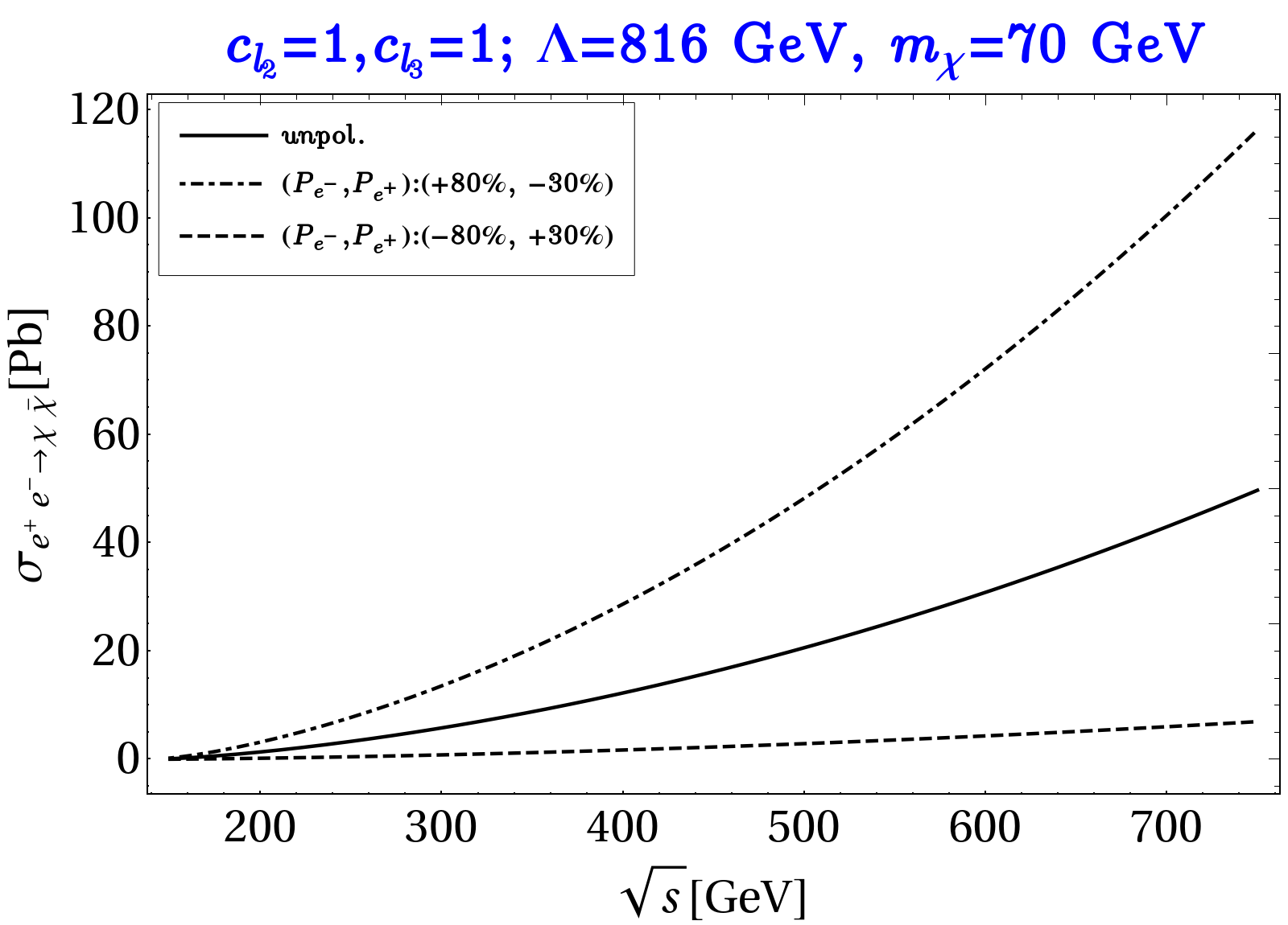
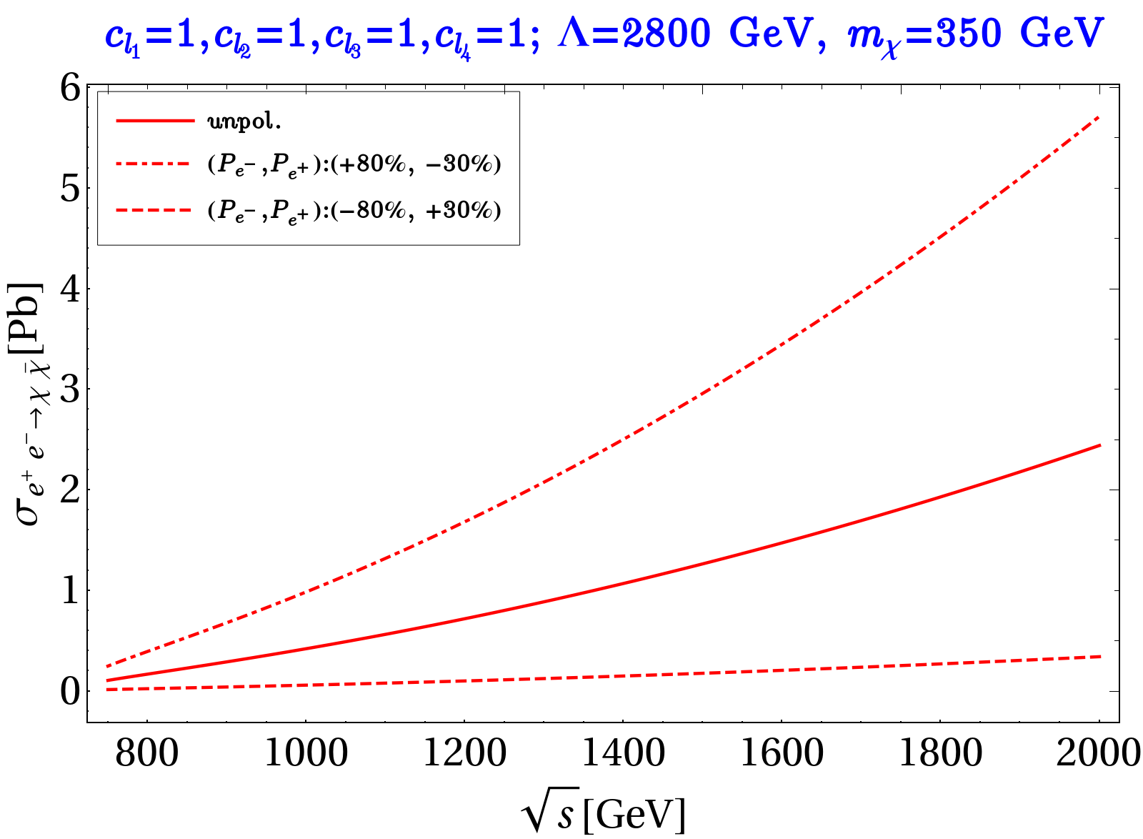
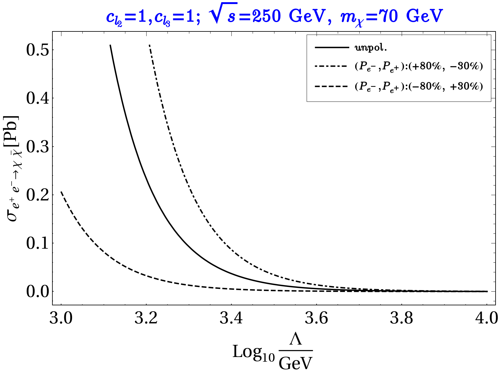
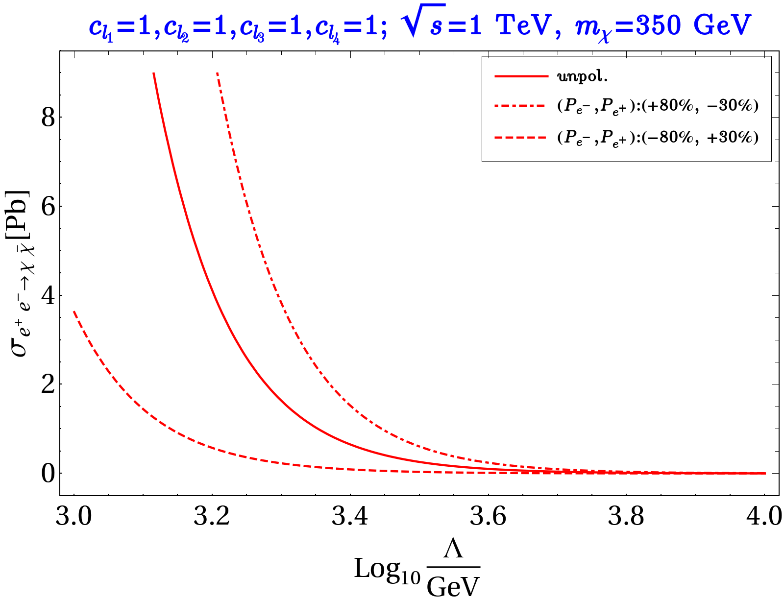
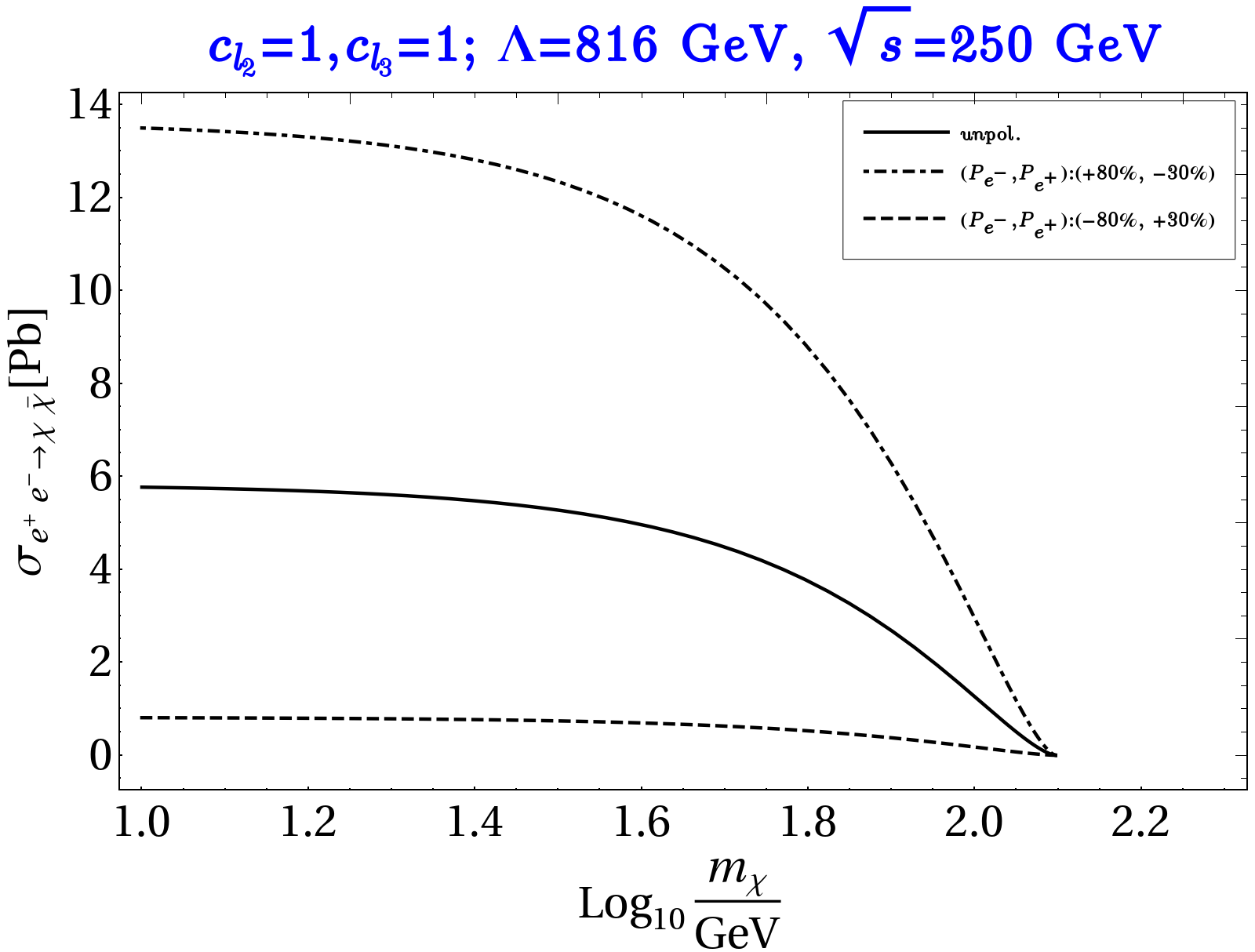
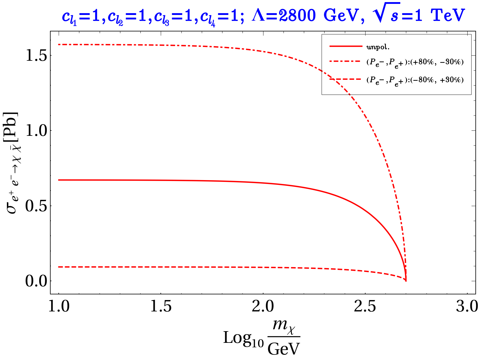
Figure 7: $\sigma_{e^{+}e^{-}\rightarrow\chi\bar{\chi}}$ as function of $\sqrt{s}$ (top panel), $\Lambda$ (middle panel) and $m_{\chi}$ (bottom panel) for Majorana DM (BP1) in the left column and Dirac DM (BP4) in the right column for three choices of polarisation: $\{P_{e^{-}}:P_{e^{+}}\}=\{0,0\};\{+0.8,-0.3\};\{-0.8,+0.3\}$ as mentioned in the figure inset. The other parameters kept fixed are mentioned in Figure heading.

We plot the variation of DM production cross-section ($\sigma_{e^{+}e^{-}\rightarrow\chi\bar{\chi}}$) for Majorana DM (BP1) in the left column and Dirac DM (BP4) in the right column of Fig. 7. In the top, middle and bottom panel we show the variation with respect to $\sqrt{s}$, $\Lambda$ and $m_{\chi}$ respectively each for three different choices of the beam polarization: $\{P_{e^{-}}:P_{e^{+}}\}=\{0,0\};\{+0.8,-0.3\};\{-0.8,\\ +0.3\}$ shown by solid, dashed-dot and dashed black (red) curves for Majorana (Dirac) DM cases with all accessible operators put together. The other parameters kept fixed are mentioned in the Figure headings. We find the signal cross-section to be maximum for the $\{+80\%,-30\%\}$ case as elaborated above, with all Wilson coefficients chosen positive. The shape of the plot in the left panel (for Majorana DM) and in the right panel (for Dirac DM) can be verified from the Eq. (30) and Eq. (29) respectively where we find that total cross-section to increase with the CM energy ($\sqrt{s}$) upto effective limit $\Lambda>\sqrt{s}$ (top panel). In the middle panel, the cross-section falls with larger $\Lambda$ as $\sigma_{e\bar{e}\rightarrow\chi\bar{\chi}}\sim 1/\Lambda^{4}$ for a fixed DM mass. The cross-section slowly falls with $m_{\chi}$ and vanishes for $\sqrt{s}\lesssim 2m_{\chi}$, as expected from the phase-space dependence shown in the bottom panel of Fig. 7.

  

  

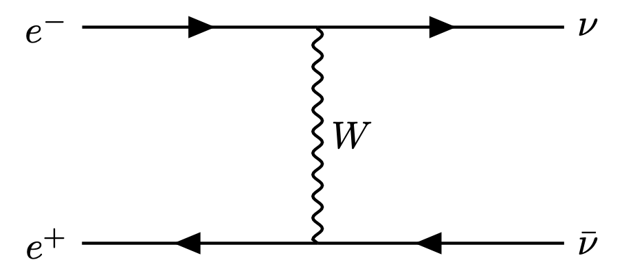
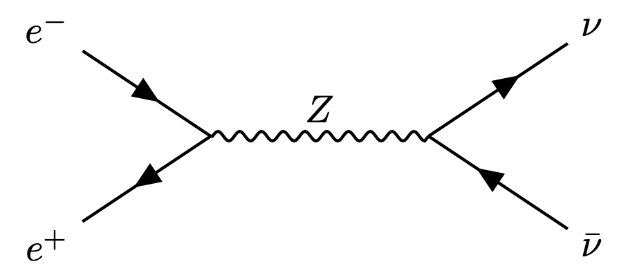
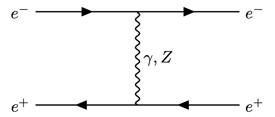
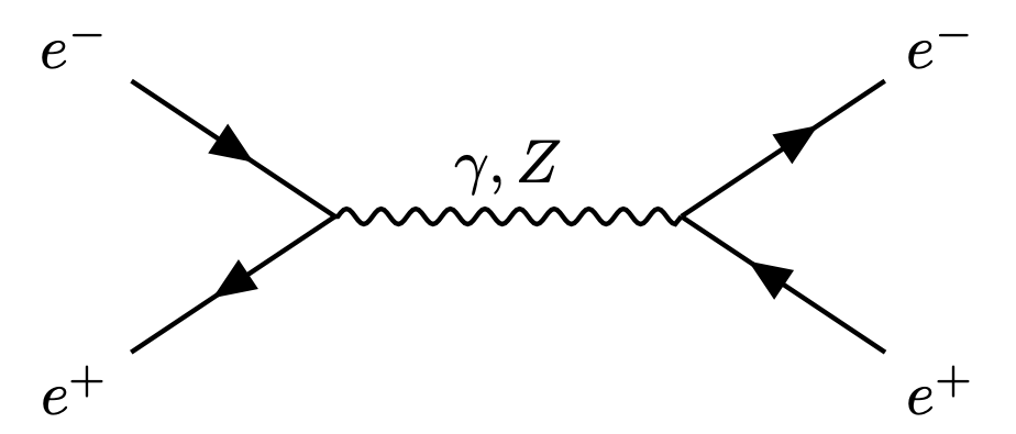
Figure 8: Top: SM background due to $e^{+}e^{-}\rightarrow\nu\bar{\nu}$ process. Bottom: Bhabha scattering contributing to the background for mono-photon with missing energy process where both $e^{+},e^{-}$ in the final state are undetected in the collider. In all cases radiative photons may arise either from the initial or final state radiation or both.

$\sqrt{s}$	$P_{e^{-}}$	$P_{e^{+}}$	$\sigma_{ee\rightarrow\nu\bar{\nu}}$	$\sigma_{ee\rightarrow ee}$
(GeV)			(pb)	(pb)
	-0.8	+0.3	102.0	618.8
250	+0.8	-0.3	14.72	628.3
	0.0	0.0	52.71	610.3
	-0.8	+0.3	130.93	622.06
1000	+0.8	-0.3	7.88	603.33
	0.0	0.0	56.03	596.29

Table 5: Production cross-section for dominant SM backgrounds at $\sqrt{s}=$ 250 and 1000 GeV.

Since we are typically interested in mono-photon signal with missing energy at the $e^{+}e^{-}$ collider, there are two main SM backgrounds which can mimic such a signal final state

• $e^{+}e^{-}\rightarrow\nu\bar{\nu}\gamma$ is an irreducible background Liu:2019ogn since neutrinos will also be missed inside the detector like the DM. Such a process is contributed by two Feynman diagrams: one involves the $t$-channel $W$ boson exchange and the other involves the $s$-channel $Z$ boson exchange as shown in the top panel of Fig. 8.

• Another possible background is the radiative Bhabha scattering $e^{+}e^{-}\rightarrow e^{+}e^{-}\gamma$ as shown in the bottom panel of Fig. 8, where both the final state leptons go undetected. Note here, that $e^{+}e^{-}\rightarrow f\bar{f}\gamma$ where $f$ is any SM fermion, lepton or jet forms a subset for this class of backgrounds, where $f$ has to be missed in the detector.

We tabulate the production cross-section dominant SM background in table 5 for different choices of the beam polarizations which can be realized in ILC set-up. The SM background contribution varies quite differently with polarization. This can be understood easily. For $e^{+}e^{-}\rightarrow\nu\bar{\nu}$, the Feynman diagrams involving $t$-channel $W$ boson exchange only contributes to a non-zero $\sigma_{\text{LR}}$ since only left-handed fermions and right-handed anti-fermions take part in the weak charge current interaction. This indicates that the asymmetry parameter $\mathcal{A}_{\text{LR}}=1$. For the $s$-channel diagram for $e^{+}e^{-}\rightarrow\nu\bar{\nu}$, exchange of a vector boson ($Z$-boson) ensures non-zero $\sigma_{\text{LR,RL}}$ due to spin conservation. Since the coupling of $Z$-boson to $e_{L}^{-}e_{R}^{+}$ is stronger than $e_{R}^{-}e_{L}^{+}$, the diagrams involving $s$-channel $Z$-exchange has more contributions to $\sigma_{\text{LR}}$ than to $\sigma_{\text{RL}}$. Therefore, for $\sigma_{e^{+}e^{-}\rightarrow\nu\bar{\nu}}$ diminishes for polarization configuration $\{P_{e^{-}}:P_{e^{+}}\}=\{+0.8,-0.3\}$, contrary to the signal for operators with all positive Wilson coefficients, which provides the best way to probe leptophilic DM at ILC. Bhaba scattering ($e^{+}e^{-}\rightarrow e^{+}e^{-}\gamma$) cross-section although still looks quite substantial, but we will be able to tame it down significantly, which we discuss in context of the event selection criteria.

4.2 Event distribution and analysis

We generate the parton-level signal events for the benchmark points in Table 3 using the batch mode of CalcHEP-3.8.10 Belyaev:2012qa . The events are then fed to Pythia-6.4.28 Sjostrand:2006za for showering utilising in-built switches for initial and final state radiation (ISR/FSR). The SM background events are generated using MadGraph Alwall:2014hca and then the event files are again analysed through Pythia. In collider environment, we reconstruct the following objects and define a few observables as

• Lepton ($l=e,\mu$): Leptons are required to have a minimum transverse momentum $p_{T}>20$ GeV and pseudorapidity $|\eta|<2.5$. Two leptons are isolated objects if their mutual distance in the $\eta-\phi$ plane is $\Delta R=\sqrt{\left(\Delta\eta\right)^{2}+\left(\Delta\phi\right)^{2}}\geq 0.2$, while the separation between a lepton and a jet has to satisfy $\Delta R\geq 0.4$.

• Jets ($j$): All the partons within $\Delta R=0.4$ from the jet initiator cell are included to form the jets using the cone jet algorithm PYCELL built in Pythia. We require $p_{T}>10$ GeV for a clustered object to be considered as jet. Jets are isolated from unclustered objects if $\Delta R>0.4$.

• Photons ($\gamma$): Photons are identified to register in the detector with minimum energy $E_{\gamma}>0.1$ GeV.

• Unclustered Objects: All the final state objects which are neither clustered to form jets, nor identified as leptons, belong to this category. All particles with $0.5<p_{T}<20$ GeV and $|\eta|<5$, are considered as unclustered.

• Missing Transverse Energy or MET ($\not{E}_{T}$): The transverse momentum of all the missing particles (those are not registered in the detector) can be estimated from the momentum imbalance in the transverse direction associated to the visible particles. Thus MET is defined as:

  $$\not{E}_{T}=-\sqrt{(\sum_{\ell,j}p_{x})^{2}+(\sum_{\ell,j}p_{y})^{2}},$$ (36)

  where the sum runs over all visible objects that include the leptons, jets and the unclustered components.

• Missing Energy or ME ($\not{E}$): The energy which is carried away by the missing particles can be identified at lepton collider given the knowledge of CM energy of the reaction as

  $$\not{E}=\sqrt{s}-\sum_{\ell,j,\gamma}E;$$ (37)

• Missing Mass ($m_{\rm miss}$): In a leptonic collider, owing to its clean kinematics, one can introduce the Lorentz invariant “missing mass” of the system Han:2020uak . For the process $e^{+}e^{-}\rightarrow\chi\bar{\chi}\gamma$, the missing mass is inferred to be

  $$m_{\text{miss}}^{2}=(p_{e^{+}}+p_{e^{-}}-p_{\gamma})^{2}\,.$$ (38)

  In the CM frame, $m_{\rm miss}^{2}=s-2\sqrt{s}E_{\gamma}$. Here, $p_{e^{+}}$ and $p_{e^{-}}$ are the four-momenta of incoming particle beams, and $p_{\gamma}$, $E_{\gamma}$ are the four-momentum and energy of the outgoing photon respectively.

We eventually put zero lepton and jet veto on the final state events of our interest. Following detector cuts are further used on the photons identified in Pythia:

• In order to ensure most of the events are localized around the central region of the detector we choose the pseduorapidity $\left|\eta_{\gamma}\right|\leq 0.24$.

• We also ensure the final state events contain at least one “hard” photon by choosing a cut on the transverse momentum of the photons: $p_{T}^{\gamma}>5$ GeV.

    

    

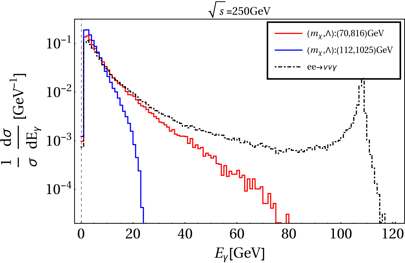
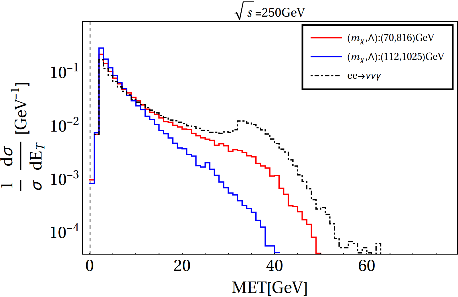
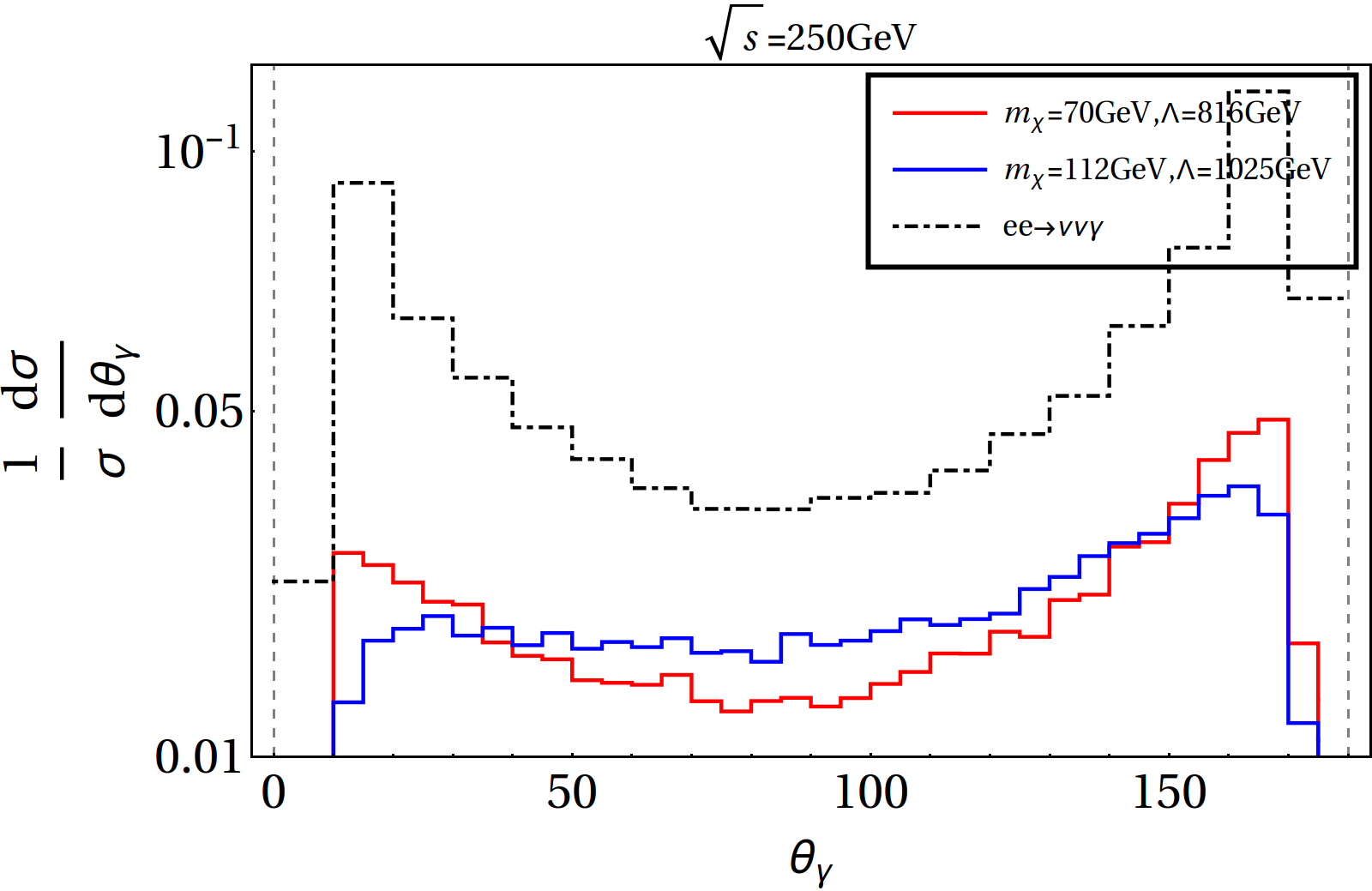
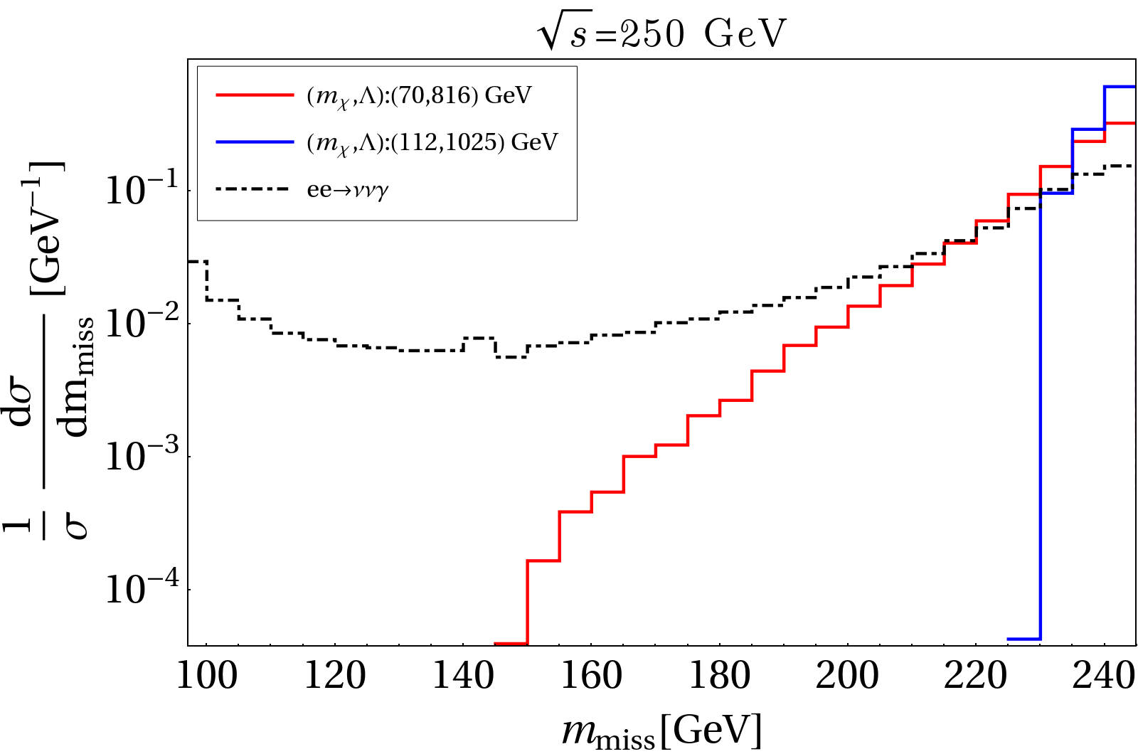
Figure 9: Top left: Normalized inclusive mono-photon event distribution for the BP1 and BP2 in table 3 and the SM backgrounds as a function of the photon energy $E_{\gamma}$. Top right: Normalized distribution of events for the signal and the SM backgrounds with missing energy (MET). Bottom left: Normalized signal and background distribution with $\theta_{\gamma}$. Bottom right: Normalized signal and SM background distribution with respect to $m_{\text{miss}}$. In all cases the signals are shown in red and blue curves, while the SM background is shown by the dashed black curve for $e^{+}e^{-}\rightarrow\nu\bar{\nu}$. We simulate the events at $\sqrt{s}=250$ GeV with $\{P_{e^{-}}:P_{e^{+}}\}=\{+0.8:-0.3\}$ beam polarization.

    

    

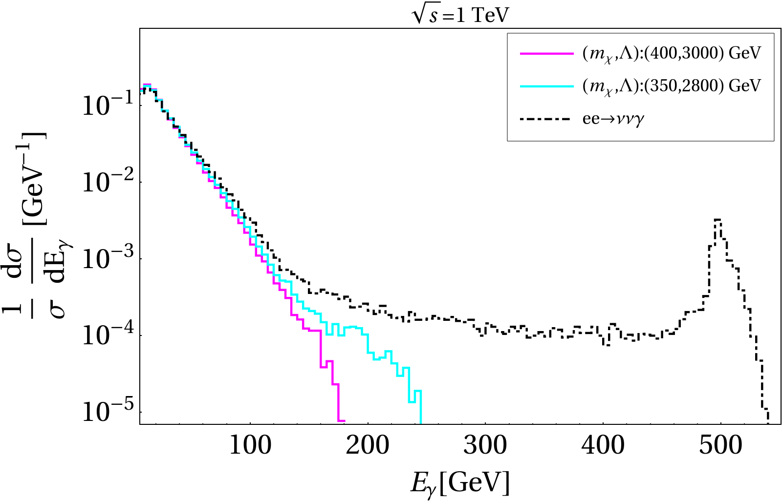
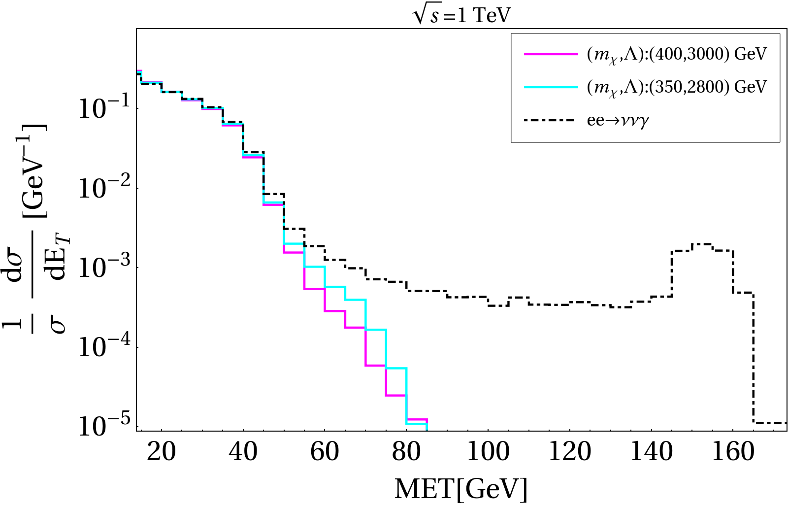
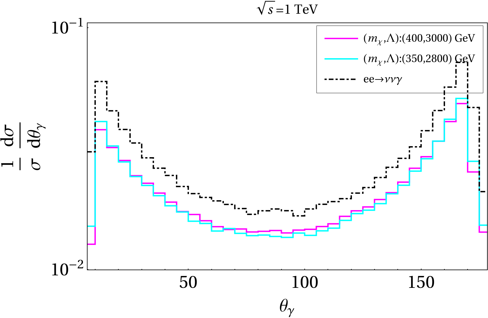
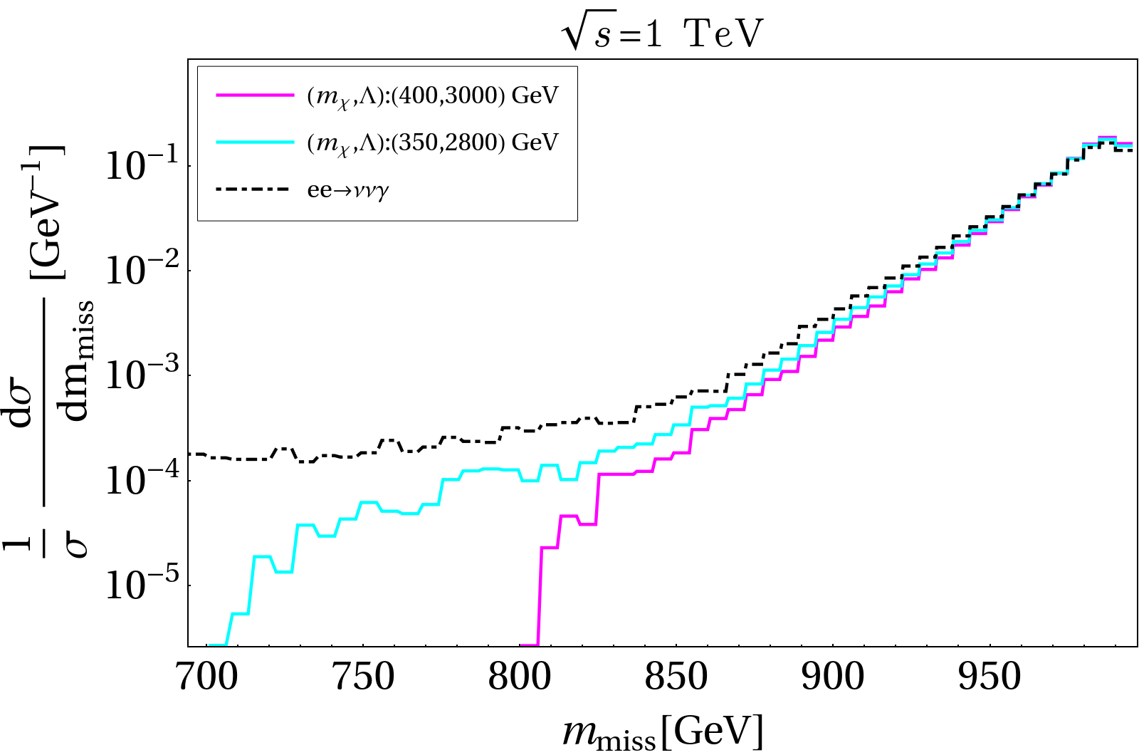
Figure 10: Same as Fig. 9 with BP4 and BP5, but with $\sqrt{s}=1$ TeV.

Due to collinear singularity, the radiative Bhabha scattering process has large cross section when both final state electron and positron go along the beam directions. However, as shown in Liu:2019ogn , such backgrounds can be efficiently removed by adopting $E_{\gamma}>E_{\text{B}}^{m}(\theta_{\gamma})$ on the final state mono photon with

$$E_{\text{B}}^{m}(\theta_{\gamma})=\sqrt{s}\Biggl{[}1+\frac{\sin\theta_{\gamma}}{\sin\theta_{\text{bnd}}}\Biggr{]}^{-1}$$ (39)

where $|\cos\theta_{\text{bnd}}|=0.99$ corresponds to the boundary of the electromagnetic calorimeter (EMC). Thus, here onwards, we will omit SM background due to Bhabha scattering process and only consider the irreducible neutrino background. We would like to further mention that this particular choice of cut on the final state mono-photon energy (Eq. (39)) also efficiently eliminates reducible backgrounds due to processes like $e^{+}\,e^{-}\rightarrow f\,\bar{f}\,\gamma$ and $e^{+}\,e^{-}\rightarrow\gamma\,\gamma\,\gamma$ as shown in Liu:2019ogn .

The distribution of normalized number of inclusive mono-photon events corresponding to the signal for Majorana DM as well as to the backgrounds, as a function of different observables, are illustrated in Fig. 9. As seen from the top left panel, the mono-photon energy $E_{\gamma}$ spectrum does not exhibit any peak structure, whereas $e^{+}e^{-}\rightarrow\nu\bar{\nu}\gamma$ shows a peak around $E_{\gamma}=\frac{s-m_{Z}^{2}}{2\sqrt{s}}$. It is easy to show from the 2-body kinematics, the maximum photon energy due to the signal is given by Liu:2019ogn

$$E_{\gamma}<E_{\chi}^{\text{max}}=\frac{1}{2\sqrt{s}}\left(s-4m_{\chi}^{2}\right)\,,$$ (40)

which exactly determines the end-point of the signal distribution. As a result, we see, for a heavier DM the radiated photons are less energetic. Note that the distribution for $E_{\gamma}$ is identical to ME ($\not{E}$) distribution given the presence of only one photon in the event. The normalized event distribution for MET (top right) are also similar to photon transverse momenta $p_{T}^{\gamma}$ for the same reason. Also a more massive DM results in a less-energetic radiated photon since most of the energy is carried by the DM itself. In the present scenario, since the photons come from the ISR, they tend to be soft and collinear. This makes their $\theta_{\gamma}$ distribution rather flat as shown in the bottom left panel. $m_{\text{miss}}$ distribution in the bottom right panel shows a clear distinction for DM signal from that of $\nu\bar{\nu}$ background, allowing to segregate them with a lower $m_{\text{miss}}$ cut, better for heavier DM mass. A similar set of distributions is shown for Dirac DM in Fig. 10, with a higher CM energy and the inferences broadly remain the same. In passing we note that the distributions as shown in Figs. 9, 10 primarily depend on the kinematics, therefore conclusions for other benchmark points as in Table 3 can be easily gauged.

4.3 Cut-flow and signal significance

Only for a small fraction of neutrino pair production events the radiated photon can be measured in the detector Kalinowski:2020lhp . Therefore, as mentioned earlier, we demand the final event selection to have photons with transverse momentum $p_{T}^{\gamma}>p_{T}^{\text{min}}=5$ GeV. On top of this we apply the following cuts in order to reduce the SM background as efficiently as possible, without harming the signal events.

• Cut1 ($\mathcal{C}_{1}$) : Events with zero lepton and jet-veto with exactly one photon in the final state.

• Cut2 ($\mathcal{C}_{2}$): We choose photons with energy lying within the window $0.1\leq E_{\gamma}<$ 60 (130) GeV or Majorana (Dirac) DM scenario. This helps to avoid the background events around the $Z$-mass window by retaining majority of the signal events.

• Cut3 ($\mathcal{C}_{3}$): We apply a cut on the missing transverse energy $\not{E_{T}}\leq$ 33 (43) GeV for for Majorana (Dirac) DM scenario.

• Cut4 ($\mathcal{C}_{4}$): Finally, we employ the missing mass cut $m_{\text{miss}}\geq$ 140 (220) GeV for BP1 (BP2), Majorana DM scenario and $m_{\text{miss}}\geq$ 700 (800) GeV for BP4 (BP5), Dirac DM scenario.

Cuts	BP1	BP2	$\nu\bar{\nu}\gamma$	$\epsilon^{\tt BP1}$	$\epsilon^{\tt BP2}$	$\sigma^{\tt BP1}=\frac{S}{\sqrt{S+B}}$	$\sigma^{\tt BP2}=\frac{S}{\sqrt{S+B}}$
	(fb)	(fb)	(fb)			$(\mathcal{L}=$ 100 $\text{fb}^{-1})$	$(\mathcal{L}=$ 100 $\text{fb}^{-1})$
$\mathcal{C}_{1}$	72.53	1.32	303.62	0.011	0.004	37.40	0.75
$\mathcal{C}_{2}$	71.99	1.31	208.91	0.011	0.004	42.95	0.90
$\mathcal{C}_{3}$	67.16	1.23	176.64	0.010	0.004	43.01	0.96
$\mathcal{C}_{4}$	67.16	1.23	133.73	0.010	0.004	47.38	1.14

Table 6: Event cross-section (fb), cut-efficiency ($\epsilon$) and signal significance $\sigma=\frac{S}{\sqrt{S+B}}$ for the benchmark points (BP1 and BP2) corresponding to Majorana DM along with the irreducible SM background for CM energy ($\sqrt{s}$) = 250 GeV with $\{P_{e^{-}}:P_{e^{+}}\}=\{+0.8:-0.3\}$ beam polarization.

Cuts	BP4	BP5	$\nu\bar{\nu}\gamma$	$\epsilon^{\tt BP4}$	$\epsilon^{\tt BP5}$	$\sigma^{\tt BP4}=\frac{S}{\sqrt{S+B}}$	$\sigma^{\tt BP5}=\frac{S}{\sqrt{S+B}}$
	(fb)	(fb)	(fb)			$(\mathcal{L}=$ 100 $\text{fb}^{-1})$	$(\mathcal{L}=$ 100 $\text{fb}^{-1})$
$\mathcal{C}_{1}$	28.20	14.17	281.36	0.035	0.030	16.02	8.24
$\mathcal{C}_{2}$	28.10	14.16	275.05	0.035	0.030	16.13	8.32
$\mathcal{C}_{3}$	27.81	14.02	268.15	0.034	0.030	16.16	8.33
$\mathcal{C}_{4}$	27.81	14.02	265.42	0.034	0.030	16.24	8.40

Table 7: Same as in Table 6, but for benchmark points (BP4, BP5) corresponding to Dirac DM scenario for CM energy ($\sqrt{s}$) = 1 TeV with $\{P_{e^{-}}:P_{e^{+}}\}=\{+0.8:-0.3\}$ beam polarization.

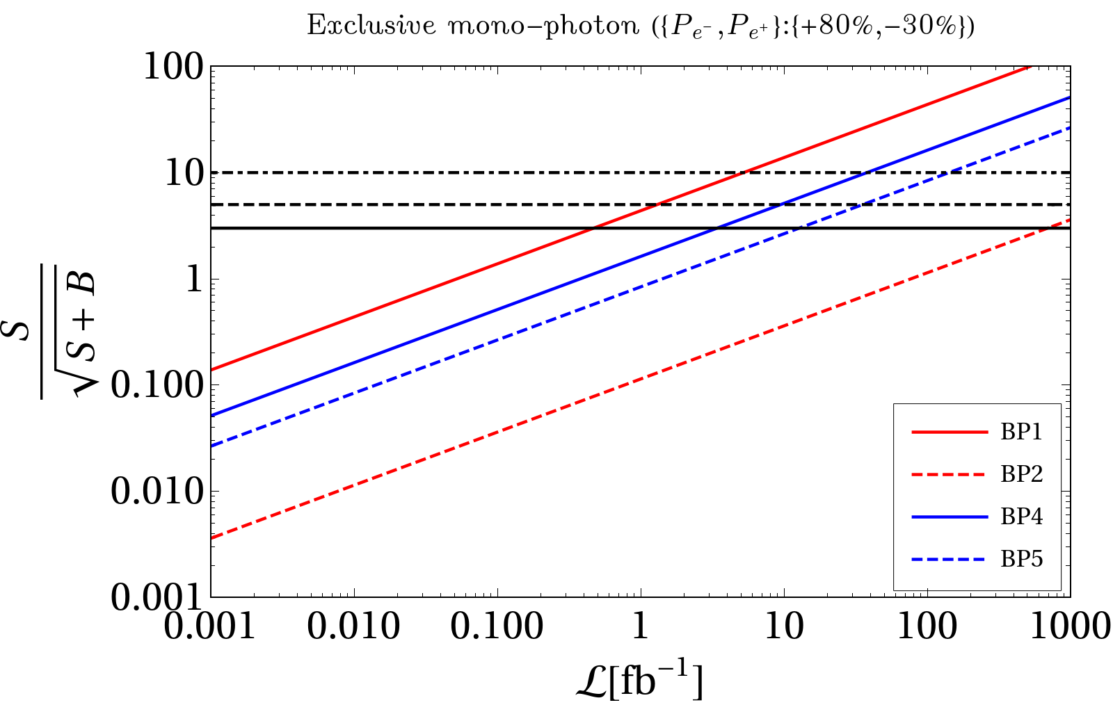
Figure 11: Signal significance for exclusive mono-photon with missing energy final state events, as a function of integrated luminosity for the chosen benchmark points in table 3. The black solid, dashed and dotdashed horizontal straight lines denote respectively 3$\sigma$, 5$\sigma$ and 10$\sigma$ discovery limit. The red (blue) lines correspond to Majorana (Dirac) DM.

In Table 6 we have tabulated the mono-photon signal for Majorana DM and background event cross-sections with the cuts employed following the sequence mentioned above. We also quote the efficiency factor $\epsilon=\frac{\sigma^{\tt sig}}{\sigma^{\tt prod}}$ (where $\sigma^{\tt prod(sig)}$ denotes the production (signal)-level cross-section), which depicts the loss of events in the process of employing selection cuts on the final state events. We also tabulate the significance of signal events with respect to SM backgrounds $\sigma=\frac{S}{\sqrt{S+B}}$ after each cuts. Here $S(=\sigma^{\tt sig}\times\mathcal{L})$ denotes the number of signal (final state) events for a given luminosity, while $B$ corresponds to the number of background events at the same luminosity. The main observations from Table 6 is that with each cut the signal significance enhances, although mildly and for the low DM mass (BP1) the significance is larger than the discovery limit with luminosity $\mathcal{L}=$ 100 $\text{fb}^{-1}$. A similar observation is made for Dirac DM from table 7, although we require higher CM energy ($\sqrt{s}$ = 1 TeV) to produce them as dictated by relic density and direct search constraints, which results both BP4 and BP5 having discovery limit at $\mathcal{L}=$ 100 $\text{fb}^{-1}$. We also see that $\epsilon$ is quite suppressed after a photon tagging (more for Majorana case), and the cut flow do not alter them significantly, which testifies that the cuts employed here retains signal to a good extent. It may also be noted that the dramatic improvement with missing mass cut as reported in Han:2020uak , is not observed in our case, owing to the limited CM energy and moderate DM mass for the chosen analysis.

The signal significance ($\sigma=\frac{S}{\sqrt{S+B}}$) is then plotted in terms of luminosity in Fig. 11. We see that mass of the DM plays a crucial role; while for a luminosity of 1 $\text{fb}^{-1}$, BP1 (red line) with $m_{\chi}=70$ GeV can reach 5$\sigma$ significance, BP2 (red dashed) with $m_{\chi}=112$ GeV requires at least $\mathcal{L}>10^{3}~{}\text{fb}^{-1}$ to be probed with 5$\sigma$ confidence. The signal cross-section for BP4 and BP5 (Dirac case) is smaller than BP1 and larger than BP2 (although with a different CM energy), so are the discovery reaches at those points, as shown by blue thick and dashed lines.

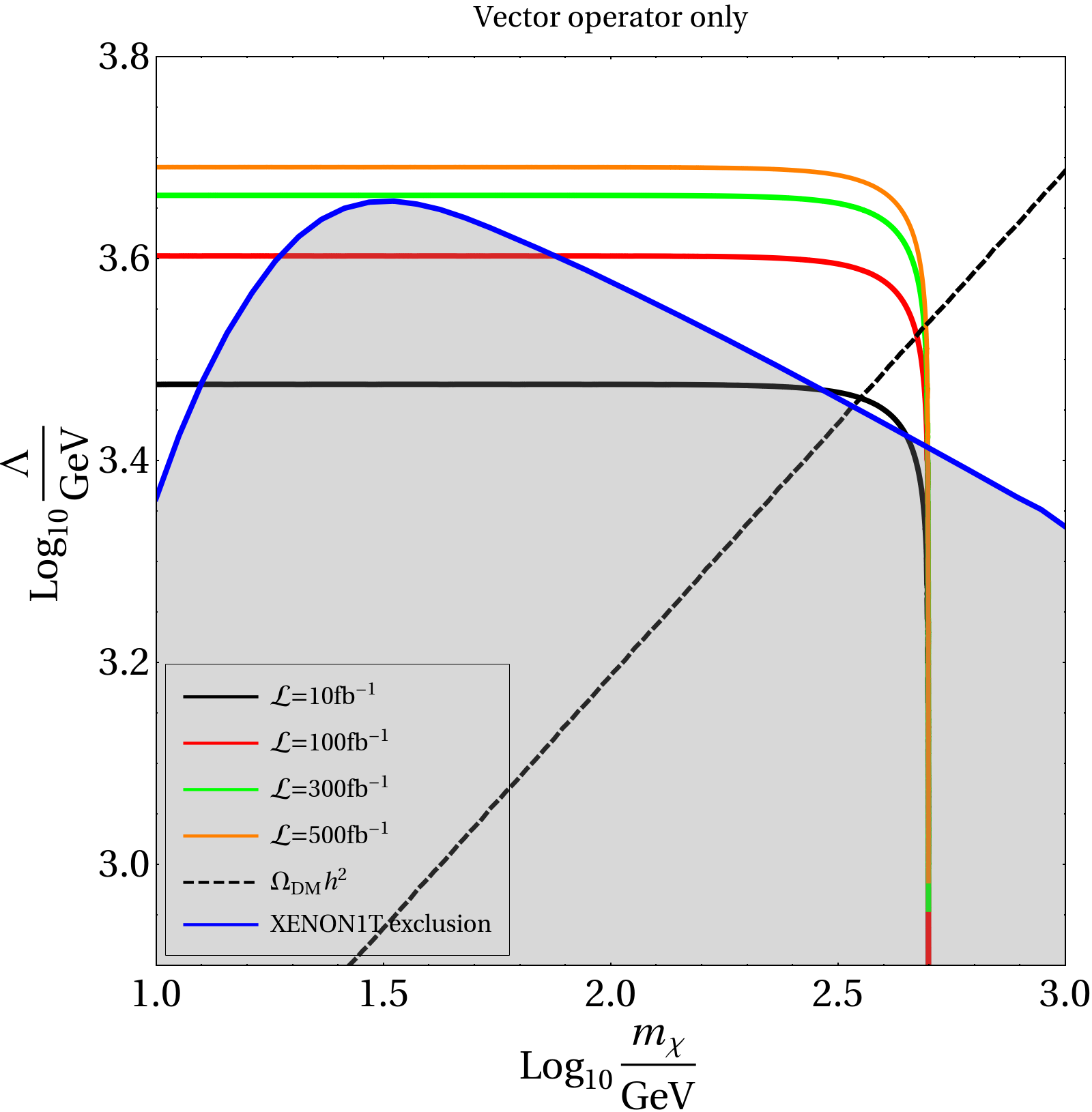
Figure 12: Parameter space in $\Lambda-m_{\chi}$ plane considering the vector operator $(\overline{\chi}\gamma^{\mu}\chi)(\overline{\ell}\gamma_{\mu}\ell)$, where the solid lines represent 3$\sigma$ significance contour for ILC at a CM energy of $\sqrt{s}=1$ TeV with integrated luminosity of $\{10,100,300,500\}\text{fb}^{-1}$ shown in black, red, green, and orange respectively; the dashed diagonal line corresponds to the Planck observed relic density for DM and the solid blue curve shows the exclusion limit from spin-independent XENON1T data.

It is useful to study the interplay of collider vs non-collider bounds in the context of effective operator as this provides information about the reach for different experiments in probing the DM parameter space. For hadrophilic DM such a study has been performed in many instances (for example, in Belyaev:2018pqr ). Here we would like to illustrate such an example by considering a single operator in action in context of leptophlic DM scenario. In Fig. 12 we show the complementarity of direct search sensitivity to that of the collider search in mono-photon final state for the operator $\mathcal{O}^{6}_{DL}$ in DM mass ($m_{\chi}$) versus NP scale ($\Lambda$) plane. The gray shaded region is discarded from the XENON1T exclusion limit, while along the black dashed straight diagonal line the Planck observed relic density is satisfied. The black, red, green and orange solid curves indicate 3$\sigma\equiv\frac{S}{\sqrt{S+B}}$ confidence limit at the ILC for a CM energy of $\sqrt{s}=1$ TeV, corresponding to luminosities $\mathcal{L}=\{10,100,300,500\}\,\text{fb}^{-1}$ respectively. Note that, all the collider confidence contours converge at $m_{\chi}\simeq\sqrt{s}/2\sim 500$ GeV for a CM energy of 1 TeV. It is easy to understand that with larger luminosity the collider sensitivity overpowers the direct detection.

5 Possible UV completion

In this section we sketch a few possible UV complete frameworks that are capable of generating leptophilic DM operators discussed so far in the draft. One of the simplest such possibilities can be found in Fox:2008kb , where the SM gauge sector is extended by a dark abelian gauge symmetry $U(1)_{\text{DS}}$. There is also a Dirac fermion $\chi$, odd under a dark sector parity, that can be a potential DM candidate (all SM fields are even under the same parity). In order to ensure the dark gauge boson $Z^{\prime}$ to be leptophilic, one has to ensure that it couples with equal and opposite charge to two generations of leptons for anomaly cancellation (for example, in a gauged $L_{i}-L_{j}$ model He:1990pn ; Ma:2001md ; Baek:2001kca ; Baek:2008nz ; Heeck:2011wj ; Das:2013jca ; Biswas:2016yan ; Duan:2017qwj ; Foldenauer:2018zrz with $i,j\in e,\mu,\tau$). The qurak interaction is prohibited since they do not carry any $L_{i}-L_{j}$ charge. At a scale $\mu\ll m_{Z^{\prime}}$, the heavy dark gauge boson can be integrated out resulting in an operator of the form $\bar{\chi}\,\Gamma\,\chi\bar{\ell}\,\Gamma^{\prime}\,\ell/m_{Z^{\prime}}^{2}$, where $\Gamma^{(^{\prime})}\equiv\{\gamma^{\mu},\gamma^{\mu}\,\gamma^{5}\}$.

Extra-dimensional model where the fermions have strong localizations at various points in the extra dimensions as2000 ; ms2000 ; Nussinov:Shrock02 furnishes another interesting possibility where the DM can couple to the leptons, while the coupling with the quarks is exponentially suppressed. Coupling fermions with appropriate kink (for one-extra dimension) or vortex (for two-extra dimensions) can localize the (zero-mode) fermions in the extra dimensions Rubakov:1983bb ; Kaplan:1995pe ; Dvali:2000ha . Assuming that the fermions have support in the interval $[0,L]$ in the extra dimensions, constraints from precision electroweak searches, flavor-changing neutral current, and collider searches can be accommodated by choosing $L^{-1}\equiv\Lambda_{L}\gtrsim 100$ TeV Delgado:1999sv ; Dobrescu01 . One appealing feature of this kind of extra-dimensional model is that the large hierarchy in SM fermion masses can be obtained by separating out the chiral parts in the extra dimension(s), without the requirement of large range of dimensionless Yukawa couplings. Furthermore, proton decay can be exponentially suppressed to safety by separating out quark and lepton wavefunctions in the extra dimensions as2000 ; bvd , although this does not hinder $n-\bar{n}$ oscillations nnb02 ; Nussinov:Shrock02 ; Wise13 ; nnblrs . Set of solutions of SM fermion wavefunction centers exists that reproduce neutrino masses and mixing, and is consistent with experimental data nuled ; barenboim01 . Therefore, if the DM candidate $\chi$ is localized near the leptons in the extra dimensions, then the experimental bound from proton decay implies that $\chi$ is separated widely from the quark wavefunctions. Hence, the Wilson coefficients of $(\bar{\chi}\Gamma_{\chi}^{\mu}\chi)(\bar{\ell}\Gamma_{\ell,\mu}\ell)$ will be unsuppressed, while the Wilson coefficients for $(\bar{\chi}\Gamma_{\chi}^{\mu}\chi)(\bar{\mathfrak{q}}\Gamma_{{\mathfrak{q}},\mu}{\mathfrak{q}})$ will be exponentially suppressed by the separation distance between the corresponding fermion wavefunctions, thereby generating an effective leptophilic interaction as we study here dmled .

6 Summary and Conclusions

Dark matter (DM) in effective theory (EFT) formalism has been studied extensively due to the unknown nature of dark sector and economy of free parameters ($m_{\chi},\Lambda$) without loss of predictability of the theory itself. However, DM operators coupling to SM quarks face severe constraints from direct DM searches as well as from LHC, caveat to appropriate validation of EFT limit at hadron collider. Leptophilic DM, on the other hand, is motivated from the fact that it not only provides a model independent way to probe DM physics in EFT formalism, but presents an opportunity to study DM production at $e^{+}e^{-}$ collider abiding the EFT limit after addressing relic density. Dirac DM operators can additionally be probed in the future sensitivities of direct search experiment via one loop interaction with the SM quarks, while Majorana DM operators remain absent in direct detection due to the Lorentz structure of the current.

We study the contribution from all possible DM operators of dimension six simultaneously, assuming the Wilson coefficients to contribute with equal strengths. Direct search for the Dirac DM is performed by taking into account the RG evolution of the Wilson coefficients from a high NP scale $\Lambda$ to low energy non-relativistic scale. We have seen that direct search constraints from latest XENON1T data constrains the Dirac DM model (with all Wilson coefficients chosen as one and having same sign) upto DM mass $\sim$400 GeV, with $\Lambda\simeq$ 3300 TeV.

Mono-photon arising from the initial state radiation (ISR), together with missing energy, turns out to be a potential signal to probe such operators at the ILC. For Dirac DM one requires higher CM energy ($\sqrt{s}=1$ TeV) satisfying the relic density and spin-independent direct search exclusion, while a comparatively lower CM energy ($\sqrt{s}=500$ GeV) is suffice to probe Majorana DM due to the absence of any direct search limit. The SM backgrounds can be tamed down moderately with judicious choice of cuts on observables like missing energy, missing mass, photon transverse momentum etc.; although $\nu\bar{\nu}$ provides a substantial irreducible contribution to such signals. The key is to choose a maximally right polarised electron beam and left polarized positron beam ($P_{e^{\pm}}=^{-30\%}_{+80\%}$), which helps to enhance the signal with positive Wilson coefficients and reduce the SM background significantly. A discovery reach of 5$\sigma$ can be achieved with luminosity $\mathcal{L}\simeq 1\,\text{fb}^{-1}$ for low mass Majorana DM ($m_{\chi}\sim 70$ GeV), while that for Dirac DM with masses above 300 GeV requires larger luminosity $\mathcal{L}\gtrsim 50\,\text{fb}^{-1}$.

Appendix A Annihilation cross-sections for leptophilic operators

In this appendix we list the annihilation cross-section times the relative velocity $v$, expanded in powers of $v$ for different leptophilic operators.

$$\big{(}\sigma v\big{)}_{{\cal O}_{DL}^{6}} =\frac{c_{\ell_{1}}^{2}}{2\pi\Lambda^{4}}m_{\chi}^{2}\sum_{\ell}\sqrt{1-\delta_{\chi\ell}^{2}}\bigg{[}\Big{(}2+\delta_{\chi\ell}^{2}\Big{)}+\frac{v^{2}}{24\Big{(}1-\delta_{\chi\ell}^{2}\Big{)}}\bigg{(}8-4\delta_{\chi\ell}^{2}+5\delta_{\chi\ell}^{4}\bigg{)}\bigg{]}+{\cal O}(v^{4}),$$ (41)

$$\big{(}\sigma v\big{)}_{{\cal O}_{L}^{6}} =\kappa^{2}\frac{c_{\ell_{2}}^{2}}{12\pi\Lambda^{4}}m_{\chi}^{2}\sum_{\ell}\sqrt{1-\delta_{\chi\ell}^{2}}\Big{(}2+\delta_{\chi\ell}^{2}\Big{)}v^{2}+{\cal O}(v^{4}),$$ (42)

$$\big{(}\sigma v\big{)}_{{\cal O}_{L1}^{6}} =\kappa^{2}\frac{c_{\ell_{3}}^{2}}{2\pi\Lambda^{4}}m_{\chi}^{2}\sum_{\ell}\sqrt{1-\delta_{\chi\ell}^{2}}\bigg{[}\delta_{\chi\ell}^{2}+\frac{v^{2}}{24\Big{(}1-\delta_{\chi\ell}^{2}\Big{)}}\bigg{(}8-22\delta_{\chi\ell}^{2}+17\delta_{\chi\ell}^{4}\bigg{)}\bigg{]}+{\cal O}(v^{4}),$$ (43)

$$\big{(}\sigma v\big{)}_{{\cal O}_{DL1}^{6}} =\frac{c_{\ell_{4}}^{2}}{\pi\Lambda^{4}}m_{\chi}^{2}\sum_{\ell}\bigg{[}\Big{(}1-\delta_{\chi\ell}^{2}\Big{)}^{3/2}+\frac{v^{2}}{24}\sqrt{1-\delta_{\chi\ell}^{2}}\Big{(}4+5\delta_{\chi\ell}^{2}\Big{)}\bigg{]}+{\cal O}(v^{4}),$$ (44)

where $\kappa=1(2)$ for a Dirac (Majorana) DM $\chi$, and $\delta_{\chi\ell}\equiv\frac{m_{\ell}}{m_{\chi}}$.

Appendix B Models with negative Wilson coefficients

The cases where Wilson coefficients are assumed negative (particularly for $c_{\ell_{3}}$ and $c_{\ell_{4}}$), offer different phenomenology. In this appendix, we elaborate such cases. First, we show the relic density satisfying parameter space constrained from direct detection bound from XENON1T for ($1,1,1,-1$), ($1,1,-1,1$), and $(1,1,-1,-1)$ choices of the $c_{\ell_{i}}$ for Dirac DM. To compare this with the BPs of the collider analyses in the text, we choose a few benchmark points as shown in Table 8.

$c_{\ell_{i}}$	($m_{\chi},\Lambda$) (GeV)
$(1,1,1,-1)$	($350,3300$)
$(1,1,-1,1)$	($350,2800$)
$(1,1,-1,-1)$	($350,3300$)

Table 8: Benchmark points for Dirac DM for negative choices of the Wilson coefficients $c_{\ell_{3}}$ and/or $c_{\ell_{4}}$.

The DM relic density and direct search allowed parameter space is shown in Fig. 13. The blue, and green points satisfy XENON1T bound on the spin-independent direct detection cross-section, while the red and purple points are ruled out from the same. The cross-over point from red to blue is $(275,2950)$ GeV, and similar cross-over point for purple to green is $(345,2800)$ GeV.

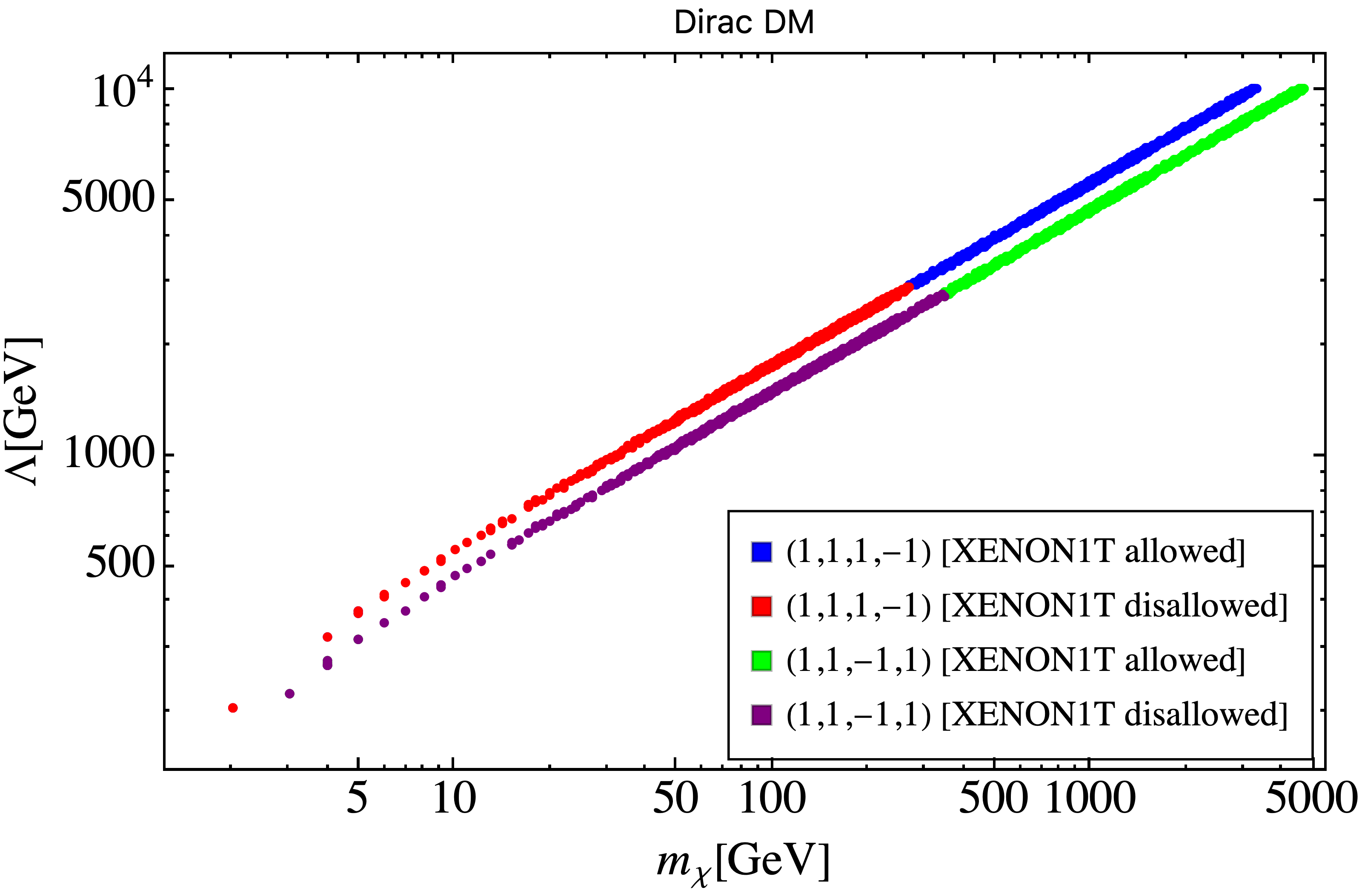
Figure 13: Relic density satisfying parameter space for different choices of the Wilson coefficients. The coupling values $(c_{\ell_{1}},c_{\ell_{2}},c_{\ell_{3}},c_{\ell_{4}})$ is denoted as an ordered set. XENON1T disallowed parameter space is marked in separate colour (see figure inset). The case $(1,1,-1,-1)$ is not shown here as it is approximately degenerate with the $(1,1,1,-1)$ case.

We plot next the variation of DM production cross-section ($\sigma_{e^{+}e^{-}\rightarrow\chi\bar{\chi}}$) for Majorana DM in the left column and Dirac DM in the right column of Fig. 14. In the top, middle and bottom panel we show the variation with respect to $\sqrt{s}$, $\Lambda$ and $m_{\chi}$ respectively for three different choices of the beam polarization: $\{P_{e^{-}}:P_{e^{+}}\}=\{0,0\};\{+0.8,-0.3\};\{-0.8,\\ +0.3\}$ shown by solid, dashed-dot and dashed black (red) curves for Majorana (Dirac) DM cases with operators having negative Wilson coefficients. See Figure caption for details. The features remain almost the same, excepting for the fact that cross-section for this case enhances for other polarization configuration, namely $\{P_{e^{-}}:P_{e^{+}}\}=\{-0.8,+0.3\}$, unlike the cases with positive Wilson coefficients. Recall, that we could reduce the neutrino background significantly using the other polarisation $\{P_{e^{-}}:P_{e^{+}}\}=\{+0.8,-0.3\}$, which reduces the signal with this particular choices of Wilson coefficients. That is why, such a possibility is harder to probe at ILC.

    

    

    

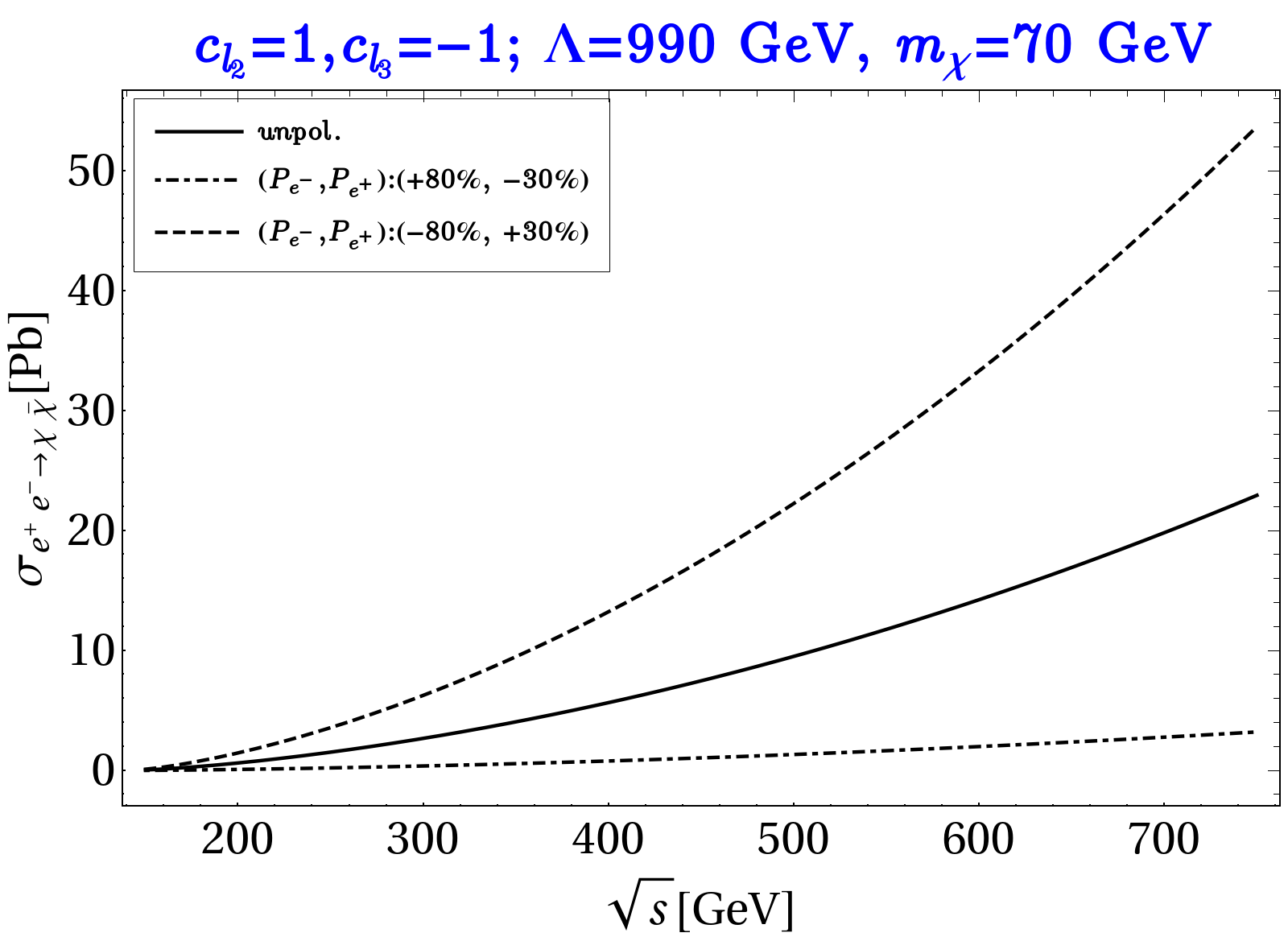
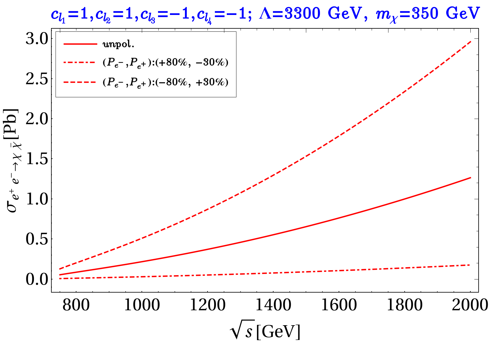
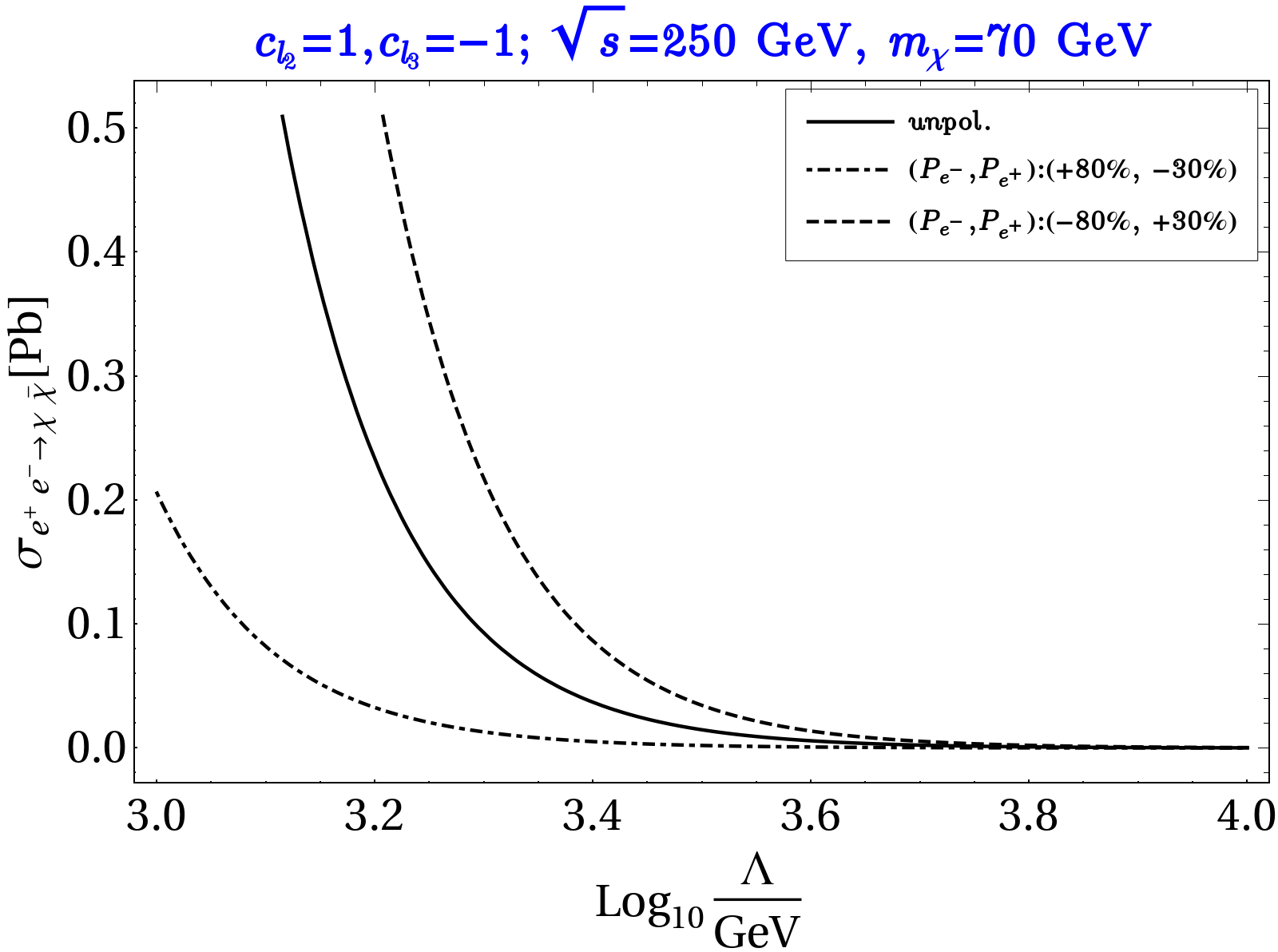
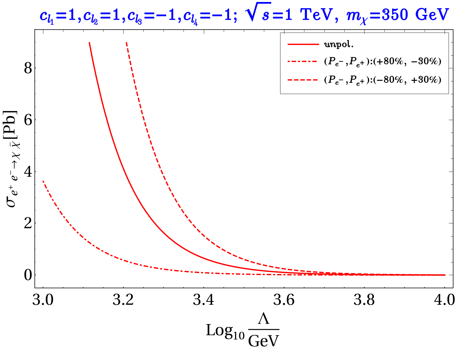
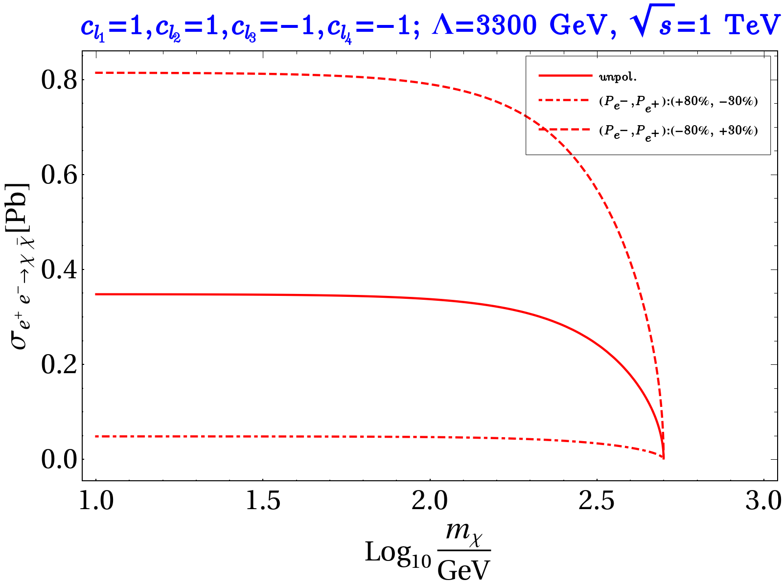
Figure 14: $\sigma_{e^{+}e^{-}\rightarrow\chi\bar{\chi}}$ as function of $\sqrt{s}$ (top panel), $\Lambda$ (middle panel) and $m_{\chi}$ (bottom panel) for Majorana DM (BP3) in the left column and Dirac DM (BP6) in the right column for three choices of polarisation: $\{P_{e^{-}}:P_{e^{+}}\}=\{0,0\};\{+0.8,-0.3\};\{-0.8,+0.3\}$ as mentioned in the figure inset. The other parameters kept fixed are mentioned in Figure heading.

References

- (1) F. Zwicky, Die Rotverschiebung von extragalaktischen Nebeln, Helv. Phys. Acta 6 (1933) 110.
- (2) F. Zwicky, On the Masses of Nebulae and of Clusters of Nebulae, Astrophys. J. 86 (1937) 217.
- (3) V. C. Rubin and W. K. Ford, Jr., Rotation of the Andromeda Nebula from a Spectroscopic Survey of Emission Regions, Astrophys. J. 159 (1970) 379.
- (4) D. Clowe, M. Bradac, A. H. Gonzalez, M. Markevitch, S. W. Randall, C. Jones et al., A direct empirical proof of the existence of dark matter, Astrophys. J. Lett. 648 (2006) L109 [astro-ph/0608407].
- (5) W. Hu and S. Dodelson, Cosmic microwave background anisotropies, Ann. Rev. Astron. Astrophys. 40 (2002) 171 [astro-ph/0110414].
- (6) Planck collaboration, Planck 2018 results. VI. Cosmological parameters, Astron. Astrophys. 641 (2020) A6 [1807.06209].
- (7) G. Jungman, M. Kamionkowski and K. Griest, Supersymmetric dark matter, Phys. Rept. 267 (1996) 195 [hep-ph/9506380].
- (8) G. Bertone, D. Hooper and J. Silk, Particle dark matter: Evidence, candidates and constraints, Phys. Rept. 405 (2005) 279 [hep-ph/0404175].
- (9) J. L. Feng, Dark Matter Candidates from Particle Physics and Methods of Detection, Ann. Rev. Astron. Astrophys. 48 (2010) 495 [1003.0904].
- (10) E. W. Kolb and M. S. Turner, The Early Universe, Front. Phys. 69 (1990) 1.
- (11) G. Arcadi, P. Ghosh, Y. Mambrini, M. Pierre and F. S. Queiroz, portal to Chern-Simons Dark Matter, JCAP 1711 (2017) 020 [1706.04198].
- (12) L. Roszkowski, E. M. Sessolo and S. Trojanowski, WIMP dark matter candidates and searches—current status and future prospects, Rept. Prog. Phys. 81 (2018) 066201 [1707.06277].
- (13) L. J. Hall, K. Jedamzik, J. March-Russell and S. M. West, Freeze-In Production of FIMP Dark Matter, JHEP 03 (2010) 080 [0911.1120].
- (14) N. Bernal, M. Heikinheimo, T. Tenkanen, K. Tuominen and V. Vaskonen, The Dawn of FIMP Dark Matter: A Review of Models and Constraints, Int. J. Mod. Phys. A32 (2017) 1730023 [1706.07442].
- (15) Y. Hochberg, E. Kuflik, T. Volansky and J. G. Wacker, Mechanism for Thermal Relic Dark Matter of Strongly Interacting Massive Particles, Phys. Rev. Lett. 113 (2014) 171301 [1402.5143].
- (16) S. Bhattacharya and J. Wudka, Effective Theories with Dark Matter Applications, 2104.01788.
- (17) A. L. Fitzpatrick, W. Haxton, E. Katz, N. Lubbers and Y. Xu, Model Independent Direct Detection Analyses, 1211.2818.
- (18) A. L. Fitzpatrick, W. Haxton, E. Katz, N. Lubbers and Y. Xu, The Effective Field Theory of Dark Matter Direct Detection, JCAP 02 (2013) 004 [1203.3542].
- (19) M. Cirelli, E. Del Nobile and P. Panci, Tools for model-independent bounds in direct dark matter searches, JCAP 10 (2013) 019 [1307.5955].
- (20) SuperCDMS collaboration, Dark matter effective field theory scattering in direct detection experiments, Phys. Rev. D 91 (2015) 092004 [1503.03379].
- (21) F. Bishara, J. Brod, B. Grinstein and J. Zupan, Chiral Effective Theory of Dark Matter Direct Detection, JCAP 02 (2017) 009 [1611.00368].
- (22) A. De Simone and T. Jacques, Simplified models vs. effective field theory approaches in dark matter searches, Eur. Phys. J. C 76 (2016) 367 [1603.08002].
- (23) F. D’Eramo, B. J. Kavanagh and P. Panci, You can hide but you have to run: direct detection with vector mediators, JHEP 08 (2016) 111 [1605.04917].
- (24) J. Brod, A. Gootjes-Dreesbach, M. Tammaro and J. Zupan, Effective Field Theory for Dark Matter Direct Detection up to Dimension Seven, JHEP 10 (2018) 065 [1710.10218].
- (25) F. Bishara, J. Brod, B. Grinstein and J. Zupan, From quarks to nucleons in dark matter direct detection, JHEP 11 (2017) 059 [1707.06998].
- (26) T. Li and Y. Liao, Constraints on dimension-seven operators with a derivative in effective field theory for Dirac dark matter, Phys. Lett. B 796 (2019) 6 [1811.08200].
- (27) J. C. Criado, A. Djouadi, M. Perez-Victoria and J. Santiago, A complete effective field theory for dark matter, JHEP 07 (2021) 081 [2104.14443].
- (28) M. Beltran, D. Hooper, E. W. Kolb and Z. C. Krusberg, Deducing the nature of dark matter from direct and indirect detection experiments in the absence of collider signatures of new physics, Phys. Rev. D 80 (2009) 043509 [0808.3384].
- (29) Q.-H. Cao, C.-R. Chen, C. S. Li and H. Zhang, Effective Dark Matter Model: Relic density, CDMS II, Fermi LAT and LHC, JHEP 08 (2011) 018 [0912.4511].
- (30) C. Cheung, G. Elor, L. J. Hall and P. Kumar, Origins of Hidden Sector Dark Matter I: Cosmology, JHEP 03 (2011) 042 [1010.0022].
- (31) J. Goodman, M. Ibe, A. Rajaraman, W. Shepherd, T. M. P. Tait and H.-B. Yu, Gamma Ray Line Constraints on Effective Theories of Dark Matter, Nucl. Phys. B 844 (2011) 55 [1009.0008].
- (32) K. Cheung, P.-Y. Tseng and T.-C. Yuan, Cosmic Antiproton Constraints on Effective Interactions of the Dark Matter, JCAP 01 (2011) 004 [1011.2310].
- (33) J. Blumenthal, P. Gretskov, M. Krämer and C. Wiebusch, Effective field theory interpretation of searches for dark matter annihilation in the Sun with the IceCube Neutrino Observatory, Phys. Rev. D 91 (2015) 035002 [1411.5917].
- (34) M. Klasen, M. Pohl and G. Sigl, Indirect and direct search for dark matter, Prog. Part. Nucl. Phys. 85 (2015) 1 [1507.03800].
- (35) N. F. Bell, Y. Cai and R. K. Leane, Impact of mass generation for spin-1 mediator simplified models, JCAP 1701 (2017) 039 [1610.03063].
- (36) N. F. Bell, G. Busoni and S. Robles, Capture of Leptophilic Dark Matter in Neutron Stars, JCAP 06 (2019) 054 [1904.09803].
- (37) J. Abdallah et al., Simplified Models for Dark Matter Searches at the LHC, Phys. Dark Univ. 9-10 (2015) 8 [1506.03116].
- (38) D. Abercrombie et al., Dark Matter Benchmark Models for Early LHC Run-2 Searches: Report of the ATLAS/CMS Dark Matter Forum, Phys. Dark Univ. 27 (2020) 100371 [1507.00966].
- (39) F. Kahlhoefer, Review of LHC Dark Matter Searches, Int. J. Mod. Phys. A 32 (2017) 1730006 [1702.02430].
- (40) B. Penning, The pursuit of dark matter at colliders—an overview, J. Phys. G 45 (2018) 063001 [1712.01391].
- (41) A. Boveia and C. Doglioni, Dark Matter Searches at Colliders, Ann. Rev. Nucl. Part. Sci. 68 (2018) 429 [1810.12238].
- (42) P. D. Group, P. A. Zyla, R. M. Barnett, J. Beringer, O. Dahl, D. A. Dwyer et al., Review of Particle Physics, Progress of Theoretical and Experimental Physics 2020 (2020) [https://academic.oup.com/ptep/article-pdf/2020/8/083C01/34673722/ptaa104.pdf].
- (43) H. Dreiner, M. Huck, M. Krämer, D. Schmeier and J. Tattersall, Illuminating Dark Matter at the ILC, Phys. Rev. D 87 (2013) 075015 [1211.2254].
- (44) Y. J. Chae and M. Perelstein, Dark Matter Search at a Linear Collider: Effective Operator Approach, JHEP 05 (2013) 138 [1211.4008].
- (45) J. de Blas et al., The CLIC Potential for New Physics, 1812.02093.
- (46) M. Habermehl, M. Berggren and J. List, WIMP Dark Matter at the International Linear Collider, Phys. Rev. D 101 (2020) 075053 [2001.03011].
- (47) J. Goodman, M. Ibe, A. Rajaraman, W. Shepherd, T. M. P. Tait and H.-B. Yu, Constraints on Light Majorana dark Matter from Colliders, Phys. Lett. B 695 (2011) 185 [1005.1286].
- (48) J. Goodman, M. Ibe, A. Rajaraman, W. Shepherd, T. M. Tait and H.-B. Yu, Constraints on Dark Matter from Colliders, Phys. Rev. D 82 (2010) 116010 [1008.1783].
- (49) Y. Bai, P. J. Fox and R. Harnik, The Tevatron at the Frontier of Dark Matter Direct Detection, JHEP 12 (2010) 048 [1005.3797].
- (50) A. Rajaraman, W. Shepherd, T. M. P. Tait and A. M. Wijangco, LHC Bounds on Interactions of Dark Matter, Phys. Rev. D 84 (2011) 095013 [1108.1196].
- (51) M. R. Buckley, Asymmetric Dark Matter and Effective Operators, Phys. Rev. D 84 (2011) 043510 [1104.1429].
- (52) P. J. Fox, R. Harnik, J. Kopp and Y. Tsai, Missing Energy Signatures of Dark Matter at the LHC, Phys. Rev. D 85 (2012) 056011 [1109.4398].
- (53) H. Dreiner, D. Schmeier and J. Tattersall, Contact Interactions Probe Effective Dark Matter Models at the LHC, EPL 102 (2013) 51001 [1303.3348].
- (54) O. Buchmueller, M. J. Dolan and C. McCabe, Beyond Effective Field Theory for Dark Matter Searches at the LHC, JHEP 01 (2014) 025 [1308.6799].
- (55) A. A. Petrov and W. Shepherd, Searching for dark matter at LHC with Mono-Higgs production, Phys. Lett. B 730 (2014) 178 [1311.1511].
- (56) S. Chang, R. Edezhath, J. Hutchinson and M. Luty, Effective WIMPs, Phys. Rev. D 89 (2014) 015011 [1307.8120].
- (57) W. Altmannshofer, P. J. Fox, R. Harnik, G. D. Kribs and N. Raj, Dark Matter Signals in Dilepton Production at Hadron Colliders, Phys. Rev. D 91 (2015) 115006 [1411.6743].
- (58) N. F. Bell, Y. Cai, J. B. Dent, R. K. Leane and T. J. Weiler, Dark matter at the LHC: Effective field theories and gauge invariance, Phys. Rev. D 92 (2015) 053008 [1503.07874].
- (59) A. Belyaev, L. Panizzi, A. Pukhov and M. Thomas, Dark Matter characterization at the LHC in the Effective Field Theory approach, JHEP 04 (2017) 110 [1610.07545].
- (60) R. M. Capdevilla, A. Delgado, A. Martin and N. Raj, Characterizing dark matter at the LHC in Drell-Yan events, Phys. Rev. D 97 (2018) 035016 [1709.00439].
- (61) A. Belyaev, E. Bertuzzo, C. Caniu Barros, O. Eboli, G. Grilli Di Cortona, F. Iocco et al., Interplay of the LHC and non-LHC Dark Matter searches in the Effective Field Theory approach, Phys. Rev. D 99 (2019) 015006 [1807.03817].
- (62) P. J. Fox, R. Harnik, J. Kopp and Y. Tsai, LEP Shines Light on Dark Matter, Phys. Rev. D 84 (2011) 014028 [1103.0240].
- (63) Z.-H. Yu, Q.-S. Yan and P.-F. Yin, Detecting interactions between dark matter and photons at high energy colliders, Phys. Rev. D 88 (2013) 075015 [1307.5740].
- (64) R. Essig, J. Mardon, M. Papucci, T. Volansky and Y.-M. Zhong, Constraining Light Dark Matter with Low-Energy Colliders, JHEP 11 (2013) 167 [1309.5084].
- (65) K. Kadota and J. Silk, Constraints on Light Magnetic Dipole Dark Matter from the ILC and SN 1987A, Phys. Rev. D 89 (2014) 103528 [1402.7295].
- (66) Z.-H. Yu, X.-J. Bi, Q.-S. Yan and P.-F. Yin, Dark matter searches in the mono- channel at high energy colliders, Phys. Rev. D 90 (2014) 055010 [1404.6990].
- (67) A. Freitas and S. Westhoff, Leptophilic Dark Matter in Lepton Interactions at LEP and ILC, JHEP 10 (2014) 116 [1408.1959].
- (68) S. Dutta, D. Sachdeva and B. Rawat, Signals of Leptophilic Dark Matter at the ILC, Eur. Phys. J. C 77 (2017) 639 [1704.03994].
- (69) Z. Liu, Y.-H. Xu and Y. Zhang, Probing dark matter particles at CEPC, JHEP 06 (2019) 009 [1903.12114].
- (70) D. Choudhury and D. Sachdeva, Model independent analysis of MeV scale dark matter. II. Implications from colliders and direct detection, Phys. Rev. D 100 (2019) 075007 [1906.06364].
- (71) H. Bharadwaj and A. Goyal, Effective Field Theory approach to lepto-philic self conjugate dark matter, Chin. Phys. C 45 (2021) 023114 [2008.13621].
- (72) S. Kundu, A. Guha, P. K. Das and P. S. B. Dev, A model-independent analysis of leptophilic dark matter at future electron-positron colliders in the mono-photon and mono-Z channels, 2110.06903.
- (73) E. Bertuzzo, C. J. Caniu Barros and G. Grilli di Cortona, MeV Dark Matter: Model Independent Bounds, JHEP 09 (2017) 116 [1707.00725].
- (74) V. Gonzalez Macias and J. Wudka, Effective theories for Dark Matter interactions and the neutrino portal paradigm, JHEP 07 (2015) 161 [1506.03825].
- (75) G. Busoni, A. De Simone, E. Morgante and A. Riotto, On the Validity of the Effective Field Theory for Dark Matter Searches at the LHC, Phys. Lett. B 728 (2014) 412 [1307.2253].
- (76) G. Busoni, A. De Simone, T. Jacques, E. Morgante and A. Riotto, On the Validity of the Effective Field Theory for Dark Matter Searches at the LHC Part III: Analysis for the -channel, JCAP 09 (2014) 022 [1405.3101].
- (77) G. Busoni, A. De Simone, J. Gramling, E. Morgante and A. Riotto, On the Validity of the Effective Field Theory for Dark Matter Searches at the LHC, Part II: Complete Analysis for the -channel, JCAP 06 (2014) 060 [1402.1275].
- (78) J. L. Diaz-Cruz and E. Ma, Neutral SU(2) Gauge Extension of the Standard Model and a Vector-Boson Dark-Matter Candidate, Phys. Lett. B 695 (2011) 264 [1007.2631].
- (79) S. Matsumoto, S. Mukhopadhyay and Y.-L. S. Tsai, Singlet Majorana fermion dark matter: a comprehensive analysis in effective field theory, JHEP 10 (2014) 155 [1407.1859].
- (80) M. Duch, Effective Operators for Dark Matter Interactions, Ph.D. thesis, Warsaw U., 2014. 1410.4427.
- (81) M. Duch, B. Grzadkowski and J. Wudka, Classification of effective operators for interactions between the Standard Model and dark matter, JHEP 05 (2015) 116 [1412.0520].
- (82) V. Gonzalez Macias and J. Wudka, Effective theories for Dark Matter interactions and the neutrino portal paradigm, JHEP 07 (2015) 161 [1506.03825].
- (83) G. D’Ambrosio, G. F. Giudice, G. Isidori and A. Strumia, Minimal flavor violation: An Effective field theory approach, Nucl. Phys. B 645 (2002) 155 [hep-ph/0207036].
- (84) M. A. Fedderke, J.-Y. Chen, E. W. Kolb and L.-T. Wang, The Fermionic Dark Matter Higgs Portal: an effective field theory approach, JHEP 08 (2014) 122 [1404.2283].
- (85) F. Bishara, J. Brod, P. Uttayarat and J. Zupan, Nonstandard Yukawa Couplings and Higgs Portal Dark Matter, JHEP 01 (2016) 010 [1504.04022].
- (86) P. Gondolo and G. Gelmini, Cosmic abundances of stable particles: Improved analysis, Nucl. Phys. B 360 (1991) 145.
- (87) J. Edsjo and P. Gondolo, Neutralino relic density including coannihilations, Phys. Rev. D 56 (1997) 1879 [hep-ph/9704361].
- (88) M. Bauer and T. Plehn, Yet Another Introduction to Dark Matter: The Particle Physics Approach, vol. 959 of Lecture Notes in Physics. Springer, 2019, 10.1007/978-3-030-16234-4, [1705.01987].
- (89) G. Belanger, F. Boudjema, A. Pukhov and A. Semenov, micrOMEGAs: A Tool for dark matter studies, Nuovo Cim. C 033N2 (2010) 111 [1005.4133].
- (90) XENON collaboration, Dark Matter Search Results from a One Ton-Year Exposure of XENON1T, Phys. Rev. Lett. 121 (2018) 111302 [1805.12562].
- (91) J. Kopp, V. Niro, T. Schwetz and J. Zupan, Dama/libra data and leptonically interacting dark matter, Phys. Rev. D 80 (2009) 083502.
- (92) J. Kopp, V. Niro, T. Schwetz and J. Zupan, DAMA/LIBRA and leptonically interacting Dark Matter, Phys. Rev. D 80 (2009) 083502 [0907.3159].
- (93) Fermi-LAT collaboration, Sensitivity Projections for Dark Matter Searches with the Fermi Large Area Telescope, Phys. Rept. 636 (2016) 1 [1605.02016].
- (94) CTA Consortium collaboration, Dark Matter and Fundamental Physics with the Cherenkov Telescope Array, Astropart. Phys. 43 (2013) 189 [1208.5356].
- (95) M. Cirelli, G. Corcella, A. Hektor, G. Hutsi, M. Kadastik, P. Panci et al., PPPC 4 DM ID: A Poor Particle Physicist Cookbook for Dark Matter Indirect Detection, JCAP 03 (2011) 051 [1012.4515].
- (96) T. R. Slatyer, Indirect Detection of Dark Matter, in Theoretical Advanced Study Institute in Elementary Particle Physics: Anticipating the Next Discoveries in Particle Physics, pp. 297–353, 2018, 1710.05137, DOI.
- (97) D. Hooper, TASI Lectures on Indirect Searches For Dark Matter, PoS TASI2018 (2019) 010 [1812.02029].
- (98) MAGIC, Fermi-LAT collaboration, Limits to Dark Matter Annihilation Cross-Section from a Combined Analysis of MAGIC and Fermi-LAT Observations of Dwarf Satellite Galaxies, JCAP 02 (2016) 039 [1601.06590].
- (99) J. L. Feng, M. Kaplinghat and H.-B. Yu, Sommerfeld Enhancements for Thermal Relic Dark Matter, Phys. Rev. D 82 (2010) 083525 [1005.4678].
- (100) I. John and T. Linden, Cosmic-Ray Positrons Strongly Constrain Leptophilic Dark Matter, 2107.10261.
- (101) PandaX-4T collaboration, Dark Matter Search Results from the PandaX-4T Commissioning Run, 2107.13438.
- (102) DELPHI collaboration, Photon events with missing energy in e+ e- collisions at s**(1/2) = 130-GeV to 209-GeV, Eur. Phys. J. C 38 (2005) 395 [hep-ex/0406019].
- (103) DELPHI collaboration, Search for one large extra dimension with the DELPHI detector at LEP, Eur. Phys. J. C 60 (2009) 17 [0901.4486].
- (104) N. F. Bell, Y. Cai, R. K. Leane and A. D. Medina, Leptophilic dark matter with interactions, Phys. Rev. D 90 (2014) 035027 [1407.3001].
- (105) K. Fujii et al., The role of positron polarization for the inital GeV stage of the International Linear Collider, 1801.02840.
- (106) P. Bambade et al., The International Linear Collider: A Global Project, 1903.01629.
- (107) The International Linear Collider Technical Design Report - Volume 1: Executive Summary, 1306.6327.
- (108) A. Belyaev, N. D. Christensen and A. Pukhov, CalcHEP 3.4 for collider physics within and beyond the Standard Model, Comput. Phys. Commun. 184 (2013) 1729 [1207.6082].
- (109) T. Sjostrand, S. Mrenna and P. Z. Skands, PYTHIA 6.4 Physics and Manual, JHEP 05 (2006) 026 [hep-ph/0603175].
- (110) J. Alwall, R. Frederix, S. Frixione, V. Hirschi, F. Maltoni, O. Mattelaer et al., The automated computation of tree-level and next-to-leading order differential cross sections, and their matching to parton shower simulations, JHEP 07 (2014) 079 [1405.0301].
- (111) T. Han, Z. Liu, L.-T. Wang and X. Wang, WIMPs at High Energy Muon Colliders, Phys. Rev. D 103 (2021) 075004 [2009.11287].
- (112) J. Kalinowski, W. Kotlarski, P. Sopicki and A. F. Zarnecki, Simulating hard photon production with WHIZARD, Eur. Phys. J. C 80 (2020) 634 [2004.14486].
- (113) P. J. Fox and E. Poppitz, Leptophilic Dark Matter, Phys. Rev. D 79 (2009) 083528 [0811.0399].
- (114) X. G. He, G. C. Joshi, H. Lew and R. R. Volkas, NEW Z-prime PHENOMENOLOGY, Phys. Rev. D 43 (1991) 22.
- (115) E. Ma, D. P. Roy and S. Roy, Gauged L(mu) - L(tau) with large muon anomalous magnetic moment and the bimaximal mixing of neutrinos, Phys. Lett. B 525 (2002) 101 [hep-ph/0110146].
- (116) S. Baek, N. G. Deshpande, X. G. He and P. Ko, Muon anomalous g-2 and gauged L(muon) - L(tau) models, Phys. Rev. D 64 (2001) 055006 [hep-ph/0104141].
- (117) S. Baek and P. Ko, Phenomenology of U(1)(L(mu)-L(tau)) charged dark matter at PAMELA and colliders, JCAP 10 (2009) 011 [0811.1646].
- (118) J. Heeck and W. Rodejohann, Gauged Symmetry at the Electroweak Scale, Phys. Rev. D 84 (2011) 075007 [1107.5238].
- (119) M. Das and S. Mohanty, Leptophilic dark matter in gauged extension of MSSM, Phys. Rev. D 89 (2014) 025004 [1306.4505].
- (120) A. Biswas, S. Choubey and S. Khan, Neutrino Mass, Dark Matter and Anomalous Magnetic Moment of Muon in a Model, JHEP 09 (2016) 147 [1608.04194].
- (121) G. H. Duan, X.-G. He, L. Wu and J. M. Yang, Leptophilic dark matter in gauged model in light of DAMPE cosmic ray excess, Eur. Phys. J. C 78 (2018) 323 [1711.11563].
- (122) P. Foldenauer, Light dark matter in a gauged model, Phys. Rev. D 99 (2019) 035007 [1808.03647].
- (123) M. Duerr, P. Fileviez Perez and M. B. Wise, Gauge Theory for Baryon and Lepton Numbers with Leptoquarks, Phys. Rev. Lett. 110 (2013) 231801 [1304.0576].
- (124) P. Schwaller, T. M. P. Tait and R. Vega-Morales, Dark Matter and Vectorlike Leptons from Gauged Lepton Number, Phys. Rev. D 88 (2013) 035001 [1305.1108].
- (125) P. Fileviez Pérez, C. Murgui and A. D. Plascencia, Neutrino-Dark Matter Connections in Gauge Theories, Phys. Rev. D100 (2019) 035041 [1905.06344].
- (126) N. Arkani-Hamed and M. Schmaltz, Hierarchies without symmetries from extra dimensions, Phys. Rev. D 61 (2000) 033005.
- (127) E. A. Mirabelli and M. Schmaltz, Yukawa hierarchies from split fermions in extra dimensions, Phys. Rev. D 61 (2000) 113011.
- (128) S. Nussinov and R. Shrock, - oscillations in models with large extra dimensions, Phys. Rev. Lett. 88 (2002) 171601.
- (129) V. A. Rubakov and M. E. Shaposhnikov, Do We Live Inside a Domain Wall?, Phys. Lett. B 125 (1983) 136.
- (130) D. B. Kaplan and M. Schmaltz, Domain wall fermions and the eta invariant, Phys. Lett. B 368 (1996) 44 [hep-th/9510197].
- (131) G. R. Dvali and M. A. Shifman, Families as neighbors in extra dimension, Phys. Lett. B 475 (2000) 295 [hep-ph/0001072].
- (132) A. Delgado, A. Pomarol and M. Quiros, Electroweak and flavor physics in extensions of the standard model with large extra dimensions, JHEP 01 (2000) 030 [hep-ph/9911252].
- (133) T. Appelquist, H.-C. Cheng and B. A. Dobrescu, Bounds on universal extra dimensions, Phys. Rev. D 64 (2001) 035002.
- (134) S. Girmohanta and R. Shrock, Baryon-Number-Violating Nucleon and Dinucleon Decays in a Model with Large Extra Dimensions, Phys. Rev. D 101 (2020) 015017 [1911.05102].
- (135) S. Nussinov and R. Shrock, - oscillations in models with large extra dimensions, Phys. Rev. Lett. 88 (2002) 171601.
- (136) J. M. Arnold, B. Fornal and M. B. Wise, Simplified models with baryon number violation but no proton decay, Phys. Rev. D 87 (2013) 075004.
- (137) S. Girmohanta and R. Shrock, Nucleon decay and - oscillations in a left-right symmetric model with large extra dimensions, Phys. Rev. D 101 (2020) 095012 [2003.14185].
- (138) S. Girmohanta, R. N. Mohapatra and R. Shrock, Neutrino Masses and Mixing in Models with Large Extra Dimensions and Localized Fermions, Phys. Rev. D 103 (2021) 015021 [2011.01237].
- (139) G. Barenboim, G. C. Branco, A. d. Gouvêa and M. N. Rebelo, Neutrino masses and lepton flavor violation in thick brane scenarios, Phys. Rev. D 64 (2001) 073005.
- (140) S. Girmohanta and R. Shrock, Extra-dimensional model of dark matter, Phys. Rev. D 104 (2021) 115021 [2109.02670].