Photon and Leptons induced processes at the LHC

Abstract

We study a few basic photon- and lepton-initiated processes at the LHC which can be computed using the recently developed photon and lepton parton densities. First, we consider the production of a massive scalar particle initiated by lepton-antilepton annihilation and photon-photon fusion as representative examples of searches of exotic particles. Then we study lepton-lepton scattering, since this Standard-Model process may be observable at the LHC. We examine these processes at leading and next-to-leading order and, using the POWHEG method, we match our calculations to parton shower programs that implement the required lepton or photon initial-states. We assess the typical size of cross-sections and their uncertainties and discuss the preferred choices for the factorization scale. These processes can also be computed starting directly from the lepto-production hadronic tensor, leading to a result where some collinear-enhanced QED corrections are missing, but all strong corrections are included. Thus, we are in the unique position to perform a comparison of results obtained via the factorization approach to a calculation that does not have strong corrections. This is particularly relevant in the case of lepton-scattering, that is more abundant at lower energies where it is affected by larger strong corrections. We thus compute this process also with the hadronic-tensor method, and compare the results with those obtained with POWHEG. Finally, for some lepton-lepton scattering processes, we compare the size of the signal to the main quark-induced background, which is double Drell-Yan production, and outline a preliminary search strategy to enhance the signal to background ratio.

1 Introduction

In recent years, precise determinations of the proton Parton-Density Functions (PDFs) of the photon Manohar:2016nzj ; Manohar:2017eqh (from here on the LUX papers) and leptons Buonocore:2020nai (from here on the LUXLep paper) have appeared. These determinations (inspired by Ref. Drees:1988pp ) were based upon the comparison of the computation of a reference photon- or lepton-initiated process (from here on, $\ell/\gamma$-initiated process) in the collinear factorization approach, and in terms of the proton electromagnetic hadronic tensor

$$W_{\mu\nu}(p,q)=\frac{1}{4\pi}\int\mathrm{d}^{4}ze^{i\,q\cdot z}\langle p|[J_{\mu}(z),J_{\nu}(0)]|p\rangle,$$ (1)

where $p$ denotes the proton momentum, the bra and ket states refer to a single proton state, and we imply an average over its spin. The hadronic tensor can be expressed in terms of the electroproduction structure functions and of the proton electromagnetic form factors. We will denote this method for the computation of $\ell/\gamma$-initiated processes in hadronic collisions as the HT (for Hadronic Tensor) method.

The calculation in the factorization approach is analogous to the Weizsäcker-Williams approximation in charged particle scattering. It starts with the simple leading order (LO) approach, where one only needs the Born matrix elements for the $\ell/\gamma$-initiated process, and is easily extended to next-to-leading order (NLO) and even to higher orders, depending upon the accuracy of the available PDF. It can benefit from available packages for the computation of NLO corrections, and also for implementing NLO calculations interfaced to parton showers (NLO+PS from here on).

So far, most calculations of $\ell/\gamma$-initiated processes using the factorization approach have been performed at the LO level, with the noticeable exception of Ref. Greljo:2020tgv , where the full NLO corrections to the resonant $s$-channel leptoquark production was presented. On the other hand, the photon and lepton PDF determinations presently available have NLO accuracy. Thus it would be desirable to fully exploit them using NLO calculations. As a related point, while we have considerable experience regarding the relative size of NLO corrections in processes initiated by quarks and gluons, little is known for $\ell/\gamma$-initiated processes in hadronic collisions. In the present paper we discuss some of these processes, compute them at LO and NLO, interface the calculations to parton shower generators according to the POWHEG method Nason:2004rx ; Frixione:2007vw ; Alioli:2010xd , and study their scale uncertainties.

We remark that NLO corrections in $\ell/\gamma$-initiated processes arise in a rather peculiar way. Rather than adding gluons to the process, as perhaps one would naively expect, corrections that are formally of NLO importance arise when the incoming photons or leptons are resolved as radiation from a parton that has higher abundance in the proton. For example, if we have an incoming photon, we also have a diagram where the photon arises from quark radiation. This diagram leads to a contribution proportional to a quark density times one power of the electromagnetic coupling $\alpha$. Being a subtracted NLO contribution it does not have any logarithmic enhancement. On the other hand, the corresponding Born process multiplies a photon density, that is of the order of a quark density times one power of the electromagnetic coupling, times a collinear logarithm $L=\log(Q/\Lambda)$, where $\Lambda$ is a typical hadronic scale. Such logarithm is parametrically of the same size of the inverse of the strong coupling constant $\alpha_{s}(Q)$, so that indeed the NLO correction is suppressed by a power of $\alpha_{s}(Q)$ with respect to the Born term.

An interesting aspect of $\ell/\gamma$-initiated processes is the possibility to search for exotic signals, typically resonances, that may preferably or exclusively couple to leptons or photons. We thus consider the production of a scalar via the processes $l^{+}l^{-}\to\phi$ and $\gamma\gamma\to\phi$, study their NLO corrections and implement corresponding NLO+PS generators using the POWHEG method. In the case of the $\gamma\gamma\to\phi$ process, we can interface our POWHEG generator to both Pythia8 Sjostrand:2014zea and Herwig7 Bellm:2019zci . Incoming leptons are not handled at the moment by Pythia8, while there is a preliminary implementation in Herwig7, so, in the lepton case, we restrict ourselves to consider the latter. We can thus assess the impact of NLO corrections both in the fixed order calculation, and in the full NLO+PS implementation. It is also interesting to compare the full NLO+PS results to LO+PS ones, since often beyond the Standard Model (BSM) studies are carried out at this level.

In the LUXLep paper, it was pointed out that some Standard Model (SM) lepton-scattering processes leading to rare final states, like leptons pairs of different flavours or same sign, may actually be detectable at the LHC, and some LO cross sections for these processes were given. Here we examine this problem in more depth, by including NLO corrections and implementing an NLO+PS generator interfaced to Herwig7. The same processes can also be computed directly adopting the HT approach. We are thus in a position to compare the full NLO calculation with the HT result, thereby validating the NLO+PS approach and also the Monte Carlo implementation of lepton initiated processes.

The factorization approach is based upon an extraction of the $\ell/\gamma$ parton densities from the result of an HT calculation, neglecting terms that are beyond the required accuracy (i.e. typically beyond NLO). Thus, the HT method could be in principle more precise. However it is more cumbersome to implement and, in the case of incoming leptons, it neglects electromagnetic corrections that are included with the factorization method, namely radiation of collinear photons from the leptons entering the scattering process. Often when considering mixed electromagnetic and strong corrections, two powers of $\alpha_{s}$ are considered to be equivalent to a single power of the electromagnetic coupling constant. According to this counting, initial state electromagnetic radiation from incoming leptons should count as $\alpha L\sim\alpha/\alpha_{s}(Q)$, i.e. as NLO contributions. We are however in a position to assess the size of these effects, by generating a lepton PDF set where initial-state radiation from leptons has been turned off, and thus we can carry out a meaningful comparison of the two methods.

The paper is divided as follows. We start by discussing in Sec. 2 the production of a scalar particle either from two initial state photons, or from a lepton-antilepton pair. We discuss the size of the cross-sections and their scale uncertainties in Sec. 2.1, and present their differential distributions in Sec. 2.2 and 2.3. In Sec. 3 we discuss lepton scattering processes. We restrict ourselves to those final states that do not receive contributions from the overwhelming Drell Yan background at leading order. We discuss the corresponding production cross-sections with their uncertainty bands at LO and NLO in Sec. 3.2. We then discuss in Sec. 3.3 the cuts required to suppress large SM backgrounds and their impact on the signal. We also present a comparison to predictions obtained with the HT method. We give our conclusions in Sec. 4. Appendix A provides details about the calculation in the HT approach, including basic formulae (A.1) and the phase space (A.2). In Appendix B we describe how we include lepton mass effects to cure the final-state collinear divergences arising from photon to lepton splitting contributions in the NLO calculation.

2 $\gamma\gamma\to\phi$ and $l^{+}l^{-}\to\phi$

In order to better understand the impact of the NLO QCD corrections to $\ell/\gamma$-initiated processes we focus on a simple case, namely the production of a neutral scalar resonance which couples only either to photons or to leptons. In particular, the objective of this section is to assess the size of the NLO corrections and their dependence upon the scale choice. Furthermore, we compare selected kinematic distributions at LO and NLO matched with parton shower using the POWHEG method.

We describe the interaction among photons and the scalar resonance through the effective Lagrangian

$$\mathcal{L}_{\rm eff}^{(\gamma)}=-\frac{1}{4}\frac{g_{\gamma}}{M_{\phi}}\phi\mathcal{F}^{\mu\nu}\mathcal{F}_{\mu\nu}\,,$$ (2)

where $\mathcal{F}^{\mu\nu}$ is the electromagnetic field strength tensor, $M_{\phi}$ is the mass of the scalar resonance and $g_{\gamma}$ is a dimensionless effective coupling. For the leptons, we consider a simple effective Yukawa interaction

$$\mathcal{L}_{\rm eff}^{(\ell)}=-iy_{\ell}\phi{\bar{\ell}}\ell.$$ (3)

Our processes proceed at LO via the partonic sub-processes $\gamma\gamma\to\phi$, in one case, and $l^{\pm}l^{\mp}\to\phi$, in the other. According to the discussion given in the introduction, they receive NLO QCD corrections from the partonic processes $q\gamma\to q\phi$ (and the corresponding crossed one $q{\bar{q}}\to\gamma\phi$, which is finite) and $l^{\pm}\gamma\to l^{\pm}\phi$ respectively. In fact, while on one hand the latter processes are down by a power of $\alpha$, they are enhanced by the ratio $f_{q}/f_{\gamma}\sim 1/(\alpha L)$ and $f_{\gamma}/f_{l}\sim\alpha L/(\alpha L)^{2}=1/(\alpha L)$ respectively, resulting in an order $1/L\sim\alpha_{s}$ correction (for a more detailed discussion see the LUXLep paper).

2.1 Total cross sections and scale dependence

In order to understand the relative impact of the NLO corrections and the remaining uncertainties associated to missing higher orders, we show in Figures 1,

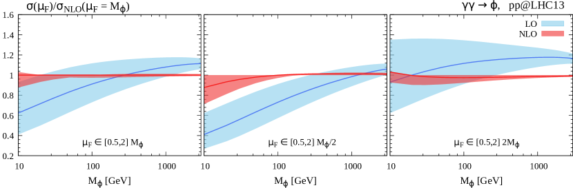
Figure 1: Comparison of LO and NLO cross sections for the photon-induced process in proton-proton collisions at $\sqrt{s}=13\,$TeV, normalised to the reference NLO cross section evaluated at $\mu_{F}=M_{\phi}$, as a function of the mass of the scalar particle. The three panels correspond to the different choices of the central scale $\mu_{0}=(1,1/2,2)M_{\phi}$. The uncertainty bands are associated to the 3-point variation of the factorization scale in the nominal range $1/2<\mu_{F}/\mu_{0}<2$.

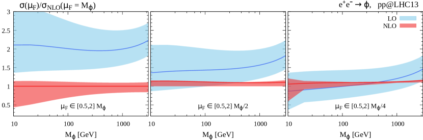
Figure 2: Comparison of LO and NLO cross sections for the lepton-induced process in proton-proton collisions at $\sqrt{s}=13\,$TeV, normalised to the reference NLO cross section evaluated at $\mu_{F}=M_{\phi}$, as a function of the mass of the scalar particle. The three panels correspond to the different choices of the central scale $\mu_{0}=(1,1/2,1/4)M_{\phi}$. The uncertainty bands are associated to the 3-point variation of the factorization scale in the nominal range $1/2<\mu_{F}/\mu_{0}<2$.

the LO and NLO cross sections for the $\gamma$-initiated process in proton-proton collisions at $\sqrt{s}=13\,$TeV, as a function of the scalar mass and for different choices of the central factorization scale, normalised to the NLO one computed at a fixed reference scale $\mu_{F}=M_{\phi}$. The analogous plot for the $\ell$-initiated process is reported in Fig. 2. Here and in the following, to obtain our results we have used the PDF set LUXlep-NNPDF31_nlo_as_0118_luxqed of Ref. Buonocore:2020nai , as implemented in LHAPDF Buckley:2014ana . The bands display the associated scale uncertainty corresponding to the 3-point variation of the factorization scale, $\mu_{\scriptscriptstyle\rm F}=(1/2,1,2)\mu_{0}$, $\mu_{0}$ being the central scale.

First, we observe that the LO result is affected by sizeable scale uncertainties which display a qualitatively similar behavior in all cases: they range from about $50\%$ at $M_{\phi}=10\,$GeV to about 5% (20%) at $M_{\phi}=2\,$TeV for the photon (lepton) induced process. The scale uncertainties shrink considerably going from LO to NLO, being of few percent (10%) for the photon (lepton) induced process, with a mild dependence upon $M_{\phi}$. Furthermore, we observe that the different scale-range choices give rather consistent results at NLO. On the other hand, we see that the LO predictions are only indicative of the cross section within a factor of order one, as is typical for LO predictions for collider processes. We find that the choice of the mass of the scalar particle as central scale is appropriate for the photon induced process, leading to K-factors around unity in the whole mass range. The situation is different for the lepton induced process, where this choice leads to large and negative corrections (K-factors $\sim 1/2$). This behavior has also been observed in the leptoquark production case Greljo:2020tgv . We also observe that in this case for the central scale $\mu_{0}=M_{\phi}$ the LO and NLO bands do not overlap. An optimal choice is provided by a smaller central scale, namely $\mu_{0}=M_{\phi}/4$. In Tab. 1, we report a collection of LO and NLO cross sections at LHC at 13 TeV for different masses of the scalar resonance, adopting the above optimal choice for the scales, and factoring out the corresponding $g_{\gamma}$ and $y_{\ell}$ couplings. We observe that photon induced cross sections at a given mass are about a factor $10^{4}$ larger than the corresponding lepton induced ones. This reflects directly the relative abundance of photons and leptons in the proton, since the two LO matrix elements have a constant ratio of order 1.

$M_{\phi}\,$[GeV]	$\sigma^{(\gamma)}_{\rm LO}/g_{\gamma}^{2}\,$[pb]	$\sigma^{(\gamma)}_{\rm NLO}/g_{\gamma}^{2}\,$[pb]	$\sigma^{(\ell)}_{\rm LO}/y_{\ell}^{2}\,$[pb]	$\sigma^{(\ell)}_{\rm NLO}/y_{\ell}^{2}\,$[pb]
$10$	$5.77^{+2.84}_{-1.97}$ $\cdot 10^{4}$	$9.26^{+0.28}_{-1.13}$ $\cdot 10^{4}$	$3.67^{+2.10}_{-2.13}$	$4.48^{+0.64}_{-1.95}$
$50$	$1.43^{+0.41}_{-0.34}$ $\cdot 10^{3}$	$1.71_{-0.04}$ $\cdot 10^{3}$	$1.07^{+0.52}_{-0.37}$ $\cdot 10^{-1}$	$1.22^{+0.04}_{-0.14}$ $\cdot 10^{-1}$
$100$	$2.26^{+0.51}_{-0.45}$ $\cdot 10^{2}$	$2.48_{-0.06}$ $\cdot 10^{2}$	$1.90^{+0.84}_{-0.62}$ $\cdot 10^{-2}$	$2.09^{+0.03}_{-0.19}$ $\cdot 10^{-2}$
$250$	$1.53^{+0.24}_{-0.23}$ $\cdot 10^{1}$	$1.54^{+0.02}_{-0.03}$ $\cdot 10^{1}$	$1.47^{+0.55}_{-0.43}$ $\cdot 10^{-3}$	$1.53_{-0.09}$ $\cdot 10^{-3}$
$500$	$1.57^{+0.19}_{-0.18}$	$1.50^{+0.02}_{-0.03}$	$1.56^{+0.53}_{-0.42}$ $\cdot 10^{-4}$	$1.55_{-0.07}$ $\cdot 10^{-4}$
$1000$	$1.17^{+0.10}_{-0.10}$ $\cdot 10^{-1}$	$1.09^{+0.01}_{-0.01}$ $\cdot 10^{-1}$	$1.11^{+0.33}_{-0.28}$ $\cdot 10^{-5}$	$1.04_{-0.03}$ $\cdot 10^{-5}$
$1500$	$2.06^{+0.15}_{-0.15}$ $\cdot 10^{-2}$	$1.88^{+0.02}_{-0.02}$ $\cdot 10^{-2}$	$1.79^{+0.50}_{-0.42}$ $\cdot 10^{-6}$	$1.59_{-0.05}$ $\cdot 10^{-6}$
$2000$	$5.14^{+0.31}_{-0.32}$ $\cdot 10^{-3}$	$4.64^{+0.05}_{-0.05}$ $\cdot 10^{-3}$	$4.04^{+1.08}_{-0.92}$ $\cdot 10^{-7}$	$3.45_{-0.13}$ $\cdot 10^{-7}$
$3000$	$5.22^{+0.24}_{-0.25}$ $\cdot 10^{-4}$	$4.69^{+0.05}_{-0.04}$ $\cdot 10^{-4}$	$3.33^{+0.82}_{-0.71}$ $\cdot 10^{-8}$	$2.65^{+0.02}_{-0.13}$ $\cdot 10^{-8}$

Table 1: LO and NLO cross sections for a heavy scalar resonance production in $\ell/\gamma$-initiated processes at the LHC at 13 TeV as a function of the mass $M_{\phi}$. The uncertainties are obtained by performing the 3-point variation around the optimal scale choices $\mu_{\scriptscriptstyle\rm F}=M_{\phi}$ for the $\gamma$-induced and $\mu_{\scriptscriptstyle\rm F}=M_{\phi}/4$ for the $\ell$-induced process, as discussed in the text.

2.2 Differential distributions for $\gamma\gamma\to\phi$

We now examine differential distributions for the photon-induced process at the level of full NLO+PS generation, that we computed using the POWHEG framework interfaced with Pythia 8.245, and Herwig 7.2 (both these generators implement processes initiated by photons Richardson:2010gz ). In our analysis we do not include multi-parton interactions, while we let the events shower and hadronize. We use Pythia8 with default parameters. As for Herwig7, we needed to set it up with customized options in order to obtain a reasonable behavior in the region of small transverse momentum of the scalar particle. In particular, we force the assignment of an intrinsic transverse momentum, whose default value is $2.2\,$GeV, also to colourless particles, which was not the case with the default Herwig7. Another important aspect, especially relevant when performing the matching at NLO, concerns the recoil scheme (see for example Ref. Cabouat:2017rzi ). Most of the NLO events are $q\gamma\to q\phi$. We remind that Pythia8 adopts by default a global recoil scheme for initial state radiation (ISR), that corresponds to an initial-initial (II) dipole setup and affects all final state particles. On the other hand, Herwig7 implements a strict dipole approach, that allows for both II and initial-final (IF) recoils. We observe that most of the time, Herwig7 treats the initial and final quark as an IF dipole, enforcing a local recoil that does not change the transverse momentum of the scalar. This leads to some distortions in the spectrum of the resonance at small $p_{T}$. For these reasons, we force a global recoil scheme also in Herwig7.

In the following, we fix the mass of the scalar to $M_{\phi}=500\,$GeV and adopt the optimal scale choice $\mu_{0}=M_{\phi}$. We show results for the transverse momentum of the resonance and of the leading and second jets. In Figs. 3 and 4 we compare leading order Pythia8 and Herwig7 predictions.

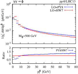
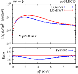
Figure 3: Transverse momentum spectrum of the scalar particle in proton-proton collisions at $\sqrt{s}=13\,$TeV for $M_{\phi}=500\,$GeV computed at leading order. The right panel shows the distributions at low $p_{T}$ values. The blue (red) line shows the prediction obtained with Pythia8 (Herwig7).

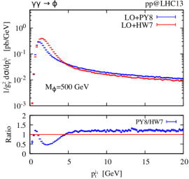
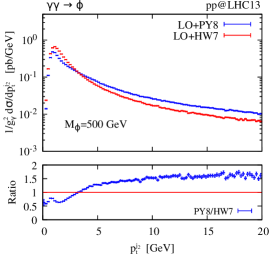
Figure 4: Transverse momentum spectrum of the leading (left panel) and second (right panel) jet in proton-proton collisions at $\sqrt{s}=13\,$TeV for $M_{\phi}=500\,$GeV computed at leading order. The blue (red) line shows the prediction obtained with Pythia8 (Herwig7).

Notice that at this order, the selected observables are entirely generated by the shower. We observe that Pythia8 tends to produce harder spectra with their peak shifted to lower $p_{T}$-values with respect to Herwig7. Overall, the differences reach about $50\%$ in both the low $p_{\rm\scriptscriptstyle T}$ and high $p_{\rm\scriptscriptstyle T}$ regions. In the former, this can be attributed to the differences among the shower and hadronization approaches, and in the latter to the different modeling of hard radiation away from the collinear region in the two generators. The same results including NLO corrections are displayed in Figs. 5 and 6. We observe a better agreement in the tails of the $p_{T}$ distributions of the resonance and of the leading jet. This is expected since these variables are now modeled by the real corrections in the fixed-order computation. Differences persist in the tail of the spectrum of the second jet, although they are milder. The shapes at small $p_{T}$ values are qualitatively similar to the pure shower results of Figs. 3 and 4.

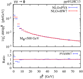
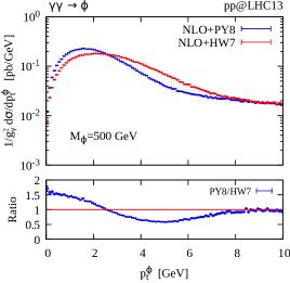
Figure 5: As in Fig. 3 computed at the NLO+PS level, comparing the prediction obtained with POWHEG+Pythia8 (blue) with POWHEG+Herwig7 (red).

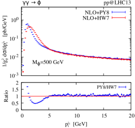
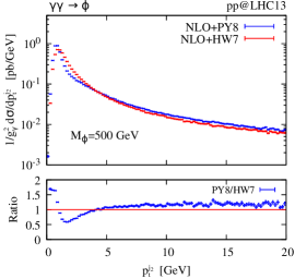
Figure 6: As in Fig. 5, for the leading (left) and second (right) jet.

In Fig. 7 and 8,

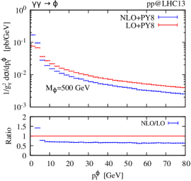
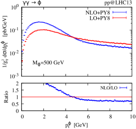
Figure 7: As in Fig. 3 comparing POWHEG+Pythia8 (blue) with Pythia8 (red).

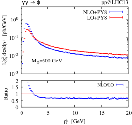
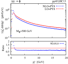
Figure 8: As in Fig. 4, comparing POWHEG+Pythia8 (blue) with Pythia8 (red).

we show a comparison between NLO+PS and LO+PS results using Pythia8. We have obtained similar results also using Herwig7. We see that the shower results provide a good qualitative description of all the considered spectra, with rather flat K-factors for moderate to high $p_{T}$-values. They tend to give harder distributions, overshooting the NLO results by a factor of almost two for transverse momenta larger than about $5\,$GeV.

Summarizing, we find considerable differences in the transverse momentum distribution of the scalar when comparing Pythia8 and Herwig7 at leading order, the Pythia8 spectrum being considerably harder. This feature is mitigated when NLO corrections are introduced, and in fact very good agreement is found both in the large transverse momentum distribution of the scalar and of the two hardest jets. On the other hand, at very low transverse momenta (i.e. $p_{T}\lesssim 10$ GeV) the two shower generators yield a very different modeling of the shape of the distributions. These features are not very relevant when searching for heavy resonances, however they give an indication that a more accurate tuning of the shower generators is needed for the modeling of $\ell/\gamma$-initiated processes. We will return to this point after the discussion of the lepton-scattering processes.

2.3 Differential distributions for $e^{+}e^{-}\to\phi$

For this process we can only use Herwig7 since Pythia8 does not currently support initial-state leptons. In Fig. 9 and 10, we show the transverse momentum of the scalar resonance and of the leading lepton, comparing the pure shower results with the NLO+PS ones using Herwig7. In this case, we find a qualitatively good agreement among them. At variance with the photon initiated process, the NLO corrections lead to a harder spectrum in both distributions. Above $20\,$GeV, we observe a rather flat K-factor of about 1.15.

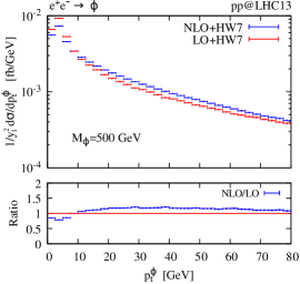
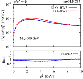
Figure 9: Transverse momentum spectrum of the scalar particle in the $\ell$-initiated production process at the $13\,$TeV LHC for $M_{\phi}=500\,$GeV. The right panel shows the distributions at low $p_{T}$ values. We compare the pure Herwig7 parton shower prediction (red) with the one obtained after the matching with the NLO computation (blue).

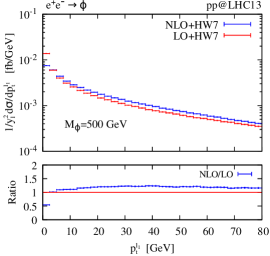
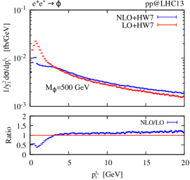
Figure 10: Transverse momentum spectrum of the leading lepton in the $\ell$-initiated scalar production process at the $13\,$TeV LHC for $M_{\phi}=500\,$GeV. The right panel shows the distributions at low $p_{T}$ values. We compare the pure Herwig7 parton shower prediction (red) with the one obtained after the matching with the NLO computation (blue).

In the region of small values of the transverse momentum of the leading lepton, we observe a discontinuity in the NLO+PS prediction related to the minimum $p_{T}$ allowed in the POWHEG generation. Again, this is not a crucial problem in the simulation of the production of high-mass states. Nonetheless, it shows the need for further investigation in the modeling of $\ell/\gamma$-initiated processes by the showers.

The shower allows us to investigate the associated hadronic activity in the event. In Fig. 11, we compare the transverse momentum of the leading leptons (hardest and next-to-hardest) with that of the leading jet. Notice that at LO+PS all the emissions are provided by the shower, while at NLO+PS the hardest emission (leading lepton) is generated according to the exact matrix element. The second lepton and leading jet, being next-to-hardest emissions, display a much softer spectrum with respect to the leading lepton, and are comparable. The shower results present a slightly harder $p_{t}$ jet spectrum, while the differences are much milder in the NLO+PS computation. The overall picture of the next-to-hardest radiation is consistent with backward evolution starting from a photon and a lepton leg. The probability to have a $q\to q\gamma$ splitting for the first and a $\gamma\to l{\bar{l}}$ for the second are in fact parametrically of the same order.

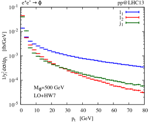
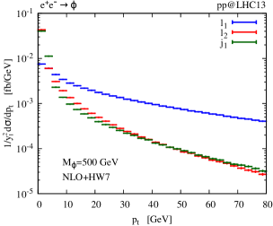
Figure 11: Transverse momentum spectrum of the leading lepton, second lepton and leading jet in the $\ell$-initiated scalar production process at the $13\,$TeV LHC for $M_{\phi}=500\,$GeV as obtained with Herwig7 (left panel) and after matching at NLO (right panel).

3 Lepton scattering

We are interested in lepton scattering processes such that the dilepton signal does not have excessive competition from other more abundant Standard Model (SM) processes. As a minimum requirement, we must focus upon final states not affected by the very large Drell-Yan background. Thus, we consider lepton pairs of different flavours or with the same electric charge. In the following we will refer to these signatures as non-Drell-Yan (NDY) pairs. We have implemented the NDY processes in the POWHEG-BOX framework, in such a way that, besides being able to compute the NLO cross sections we can also generate events to be interfaced with a shower Monte Carlo program.

As we will see in the following, the NDY processes may be observable at the LHC as long as the transverse momenta of the leptons are not too large. Thus both higher-order effects and shower details can significantly affect the result. Moreover, lepton-initiated processes have become available in shower programs only very recently, and their implementation is still in a preliminary stage. For these reasons we have also implemented a direct calculation of four lepton production using the HT (Hadronic Tensor) method, in order to better assess the reliability of our approach, and to provide a guide for the tuning of the Monte Carlos. The HT calculation is carried out by first computing the matrix element for the production of two lepton pairs, initiated by two virtual photons. This matrix element is contracted with the hadronic tensors of each incoming proton, and a full phase space integration is performed. This calculation is described in detail in appendix A.

We stress that in our HT calculation we include all contributions to the photon-induced four-leptons production, at order ${\cal O}(\alpha^{4})$. This is in contrast with the calculation of Ref. Harland-Lang:2021zvr , where diagrams of this order with the two incoming photons attached to the same fermion line are instead neglected. These contributions, not included in Ref. Harland-Lang:2021zvr , enter already in our NLO calculation (see Fig. 13, (c) and (d)) and as discussed later, are not completely negligible. Furthermore, interference terms in the case of identical fermions are never included in Ref. Harland-Lang:2021zvr .

The HT calculation includes all higher-order QCD corrections to the NDY processes. On the other hand it does not include the effect of initial-state collinear radiation of photons from leptons. These effects are of the order of the electromagnetic coupling constant $\alpha$ multiplied by a collinear logarithm $L=\log{p_{\rm\scriptscriptstyle T}}{/\Lambda}$, i.e. of order $\alpha/\alpha_{s}$, that in our counting (that is $\alpha\approx\alpha_{s}^{2}$) should be considered equivalent to an NLO correction. Rather than trying to add these effects to the HT calculation, we have estimated their size by switching them off in the calculation using the lepton PDFs by suitably adapting the Hoppet Salam:2008qg routines used in the LUXLep paper. We have found that at the transverse momenta that we have considered these effects are below the percent level, and thus we can trust the HT result for a validation of our calculations. We stress however that the HT calculation is in general much more demanding than the POWHEG NLO one. Furthermore, it cannot be straightforwardly interfaced to a shower program, and thus we have not attempted to turn it into a full event generator.

3.1 The NLO POWHEG calculation

In the left part of Fig. 12, we display one of the Feynman graph for the process of same-sign, different-flavours scattering at the Born level.

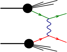
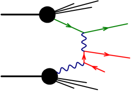
Figure 12: Left: the Born level graph for same-sign, different-flavours lepton scattering; right: an example of a real graph associated with radiative corrections to this Born graph.

We also consider same-sign identical-flavours and opposite-sign different-flavours. In the case of identical flavours an exchange graph must also be included. The NLO corrections to these processes arise from the graphs where one incoming lepton originates from an incoming photon, as shown in the right part of Fig. 12. The real graphs for the NLO corrections have several singular regions, that are shown schematically in Fig. 13,

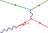
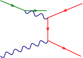
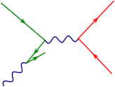
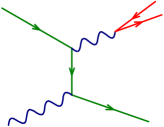
(a)	(b)	(c)	(d)

Figure 13: Singular regions associated with real graphs in the lepton scattering process.

where, for the sake of definiteness, we focus upon the scattering of leptons with different flavour. The singular regions are

1. A final-state fermion with flavour different from the incoming one becomes collinear to the incoming photon. The underlying Born for this singular region corresponds to a process of different-flavours lepton scattering, i.e. the same process that we want to include at the Born level. The corresponding collinear singularities are removed following the usual factorization procedure.

2. A final-state fermion of the same flavour of the initial one becomes collinear to it. This singular region yields a final state that is Drell-Yan like. However, this graph does contribute at the NLO level to our signal when far away from the singular region, so it must be included. Its underlying Born configuration is $\gamma\gamma\rightarrow l^{+}l^{-}$.

3. A final-state fermion with flavour equal to the incoming one becomes collinear to the incoming photon. Also in this case, the underlying Born configuration is Drell-Yan like, but away from the singular region it may contribute at the NLO level to our signal, and must be included.

4. Two opposite-flavour final-state leptons become collinear to each other. This process can generate a different-flavour pair that is not Drell-Yan like. Yet, it cannot be ascribed to a lepton scattering process, since its underlying Born is the Compton process $\gamma l\to\gamma l$. We must however include it since it is relevant at the NLO level. In order to suppress this contribution we will impose an isolation criterion upon our final leptons.

Configuration (a) is dealt with automatically by the POWHEG-BOX framework. In order to deal with the remaining singular regions, we introduce also the Born subprocesses $\gamma\gamma\rightarrow l^{+}l^{-}$, $l^{+}l^{-}\rightarrow\ell^{+}\ell^{-}$ and $l\gamma\rightarrow l\gamma$. In this way, regions (b), (c), and (d) are correctly detected as singular ones. We then use the Bornzerodamp feature of the POWHEG-BOX Melia:2011gk to separate those regions as remnants and treat them as pure unsubtracted real contributions. We notice that the divergent contributions of regions (b) and (c) are eventually excluded by the analysis cuts. On the other hand, a realistic cut to exclude region (d) would require complete isolation of the leptons. Since lepton detection cannot go below transverse momenta of the order of a GeV, a complete isolation cannot be achieved. Thus, some logarithmic sensitivity to the lepton mass remains, and we must modify the matrix elements by including mass effects in diagrams that involve the splitting of a photon into a lepton-antilepton pair. The details of our procedure are given in appendix B.

In order to deal with the remnants corresponding to regions (b), (c) and (d), that have a divergent or a logarithmically enhanced cross section, we implement their production in POWHEG with a reduced sampling rate by applying a suitable suppression factor, that is divided out from the weight of the generated event. With this procedure, if the analysis cuts are applied, we obtain correct, finite results.

3.2 NLO results and scale dependence

We begin by studying the scale dependence of the NLO cross section for all combinations of different-flavours or equal-sign lepton scattering. For completeness, we include also the contribution of $Z$ exchange and $Z\gamma$ interference. We notice that, at NLO, scattering processes of leptons of different flavours and equal or opposite charges have different cross sections even if only the electromagnetic interaction is considered. In fact, the amplitude has contributions of order $q_{l}q_{\ell}^{2}$ and $q_{\ell}q_{l}^{2}$, with $q_{l}$ and $q_{\ell}$ denoting the electric charges of the two fermions. These two contributions change relative signs if one lepton is replaced with its antilepton. On the other hand, fully charge-conjugated processes yield the same cross sections and distributions even if we include $Z$ exchange, provided we do not look at parity-sensitive observables. Thus we can omit charge-conjugate processes.

In our analysis we always consider proton-proton collisions at 13 TeV.

As discussed in the previous section, at the NLO level we must impose an isolation cut on the final-state leptons, in order to avoid the collinear divergence of the region (d). We thus require that no other lepton with transverse momentum larger than a given cut is inside a cone in the pseudorapidity-azimuthal plane with given aperture $\Delta r$. We have considered the values $\Delta r=0.1,\,0.3$ and $0.6$. We have observed a mild dependence on $\Delta r$, thus we present here only the results for $\Delta r=0.3$. Altogether, we require both leptons to satisfy the cuts

$$\begin{split}&p_{\rm\scriptscriptstyle T}>p_{\rm cut},\;p_{\rm cut}=5,10\mbox{ and }20\,{\rm GeV}\,,\qquad|\eta|<2.4\,,\\ &\mbox{isolation:}\quad\Delta r>0.3\quad\mbox{for leptons}\;p_{\rm\scriptscriptstyle T}>0.9\,{\rm GeV}\,.\end{split}$$ (4)

In figures 14, 15 and 16

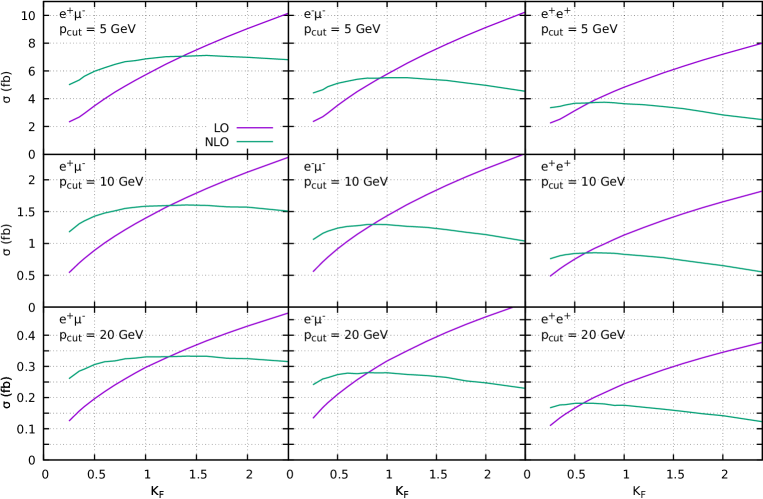
Figure 14: Scale dependence of the total cross section for lepton scattering at LO and NLO for $e^{+}\mu^{-}$, $e^{-}\mu^{-}$ and $e^{+}e^{+}$ production for different $p_{t}$ cuts.

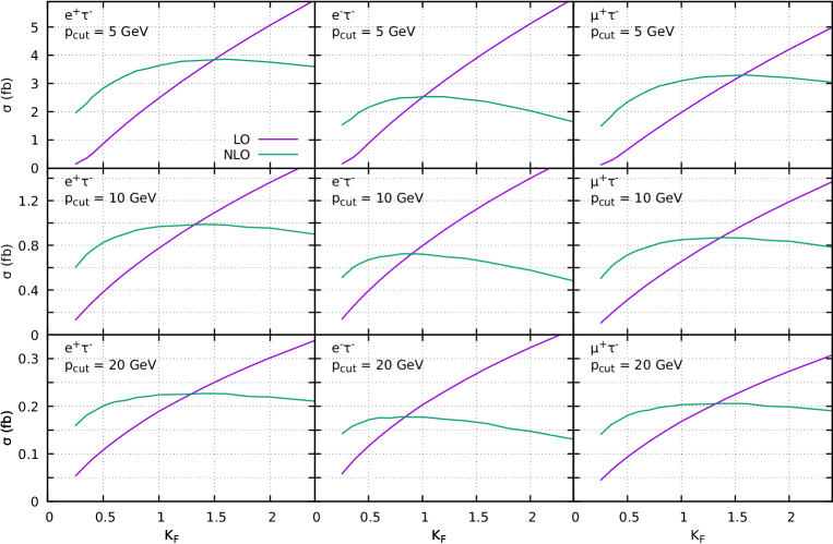
Figure 15: As Fig. 14 for $e^{+}\tau^{-}$, $e^{-}\tau^{-}$ and $\mu^{+}\tau^{-}$.

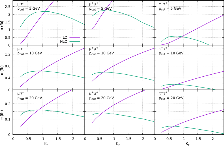
Figure 16: As Fig. 14 for $\mu^{-}\tau^{-}$, $\mu^{+}\mu^{+}$ and $\tau^{+}\tau^{+}$.

we show the cross section as a function of the factorization scale factor $K_{F}=\mu_{F}/\mu_{0}$ for different choices of the transverse momentum cut. We have chosen the reference scale $\mu_{0}$ as the sum of the absolute value of the transverse momentum of all final-state leptons divided by two. This choice is collinear-safe, since for both initial- and final-state collinear singularities it reduces to the transverse momentum of the final-state particles in the underlying Born process. We notice that, in general, there is a considerable reduction in the scale dependence when going from the LO to the NLO result. Furthermore, we observe that generally the intersection of the LO and NLO results is slightly above 1 for opposite-sign, different-flavour leptons, slightly below 1 for same-sign, different-flavour, and near 0.5 for same-sign same-flavour leptons. While the scale behaviour of the results for the electrons and muons seems very reasonable, when the $\tau$ is involved, we see an anomalously large scale dependence even at the NLO level, the worse case being $\tau\tau$ scattering. This behaviour is partly understood as a consequence of the fact that for small scales the $\tau$ parton density becomes negative, and in fact we see that for small scales the LO cross section becomes very small.

Given the differences in the scale behaviour of the different processes, we have chosen the following procedure for selecting a range of scales appropriate to each process. We have scanned the cross sections for $0.5<K_{F}<4$, with a spacing of 0.1 for $0.5<K_{F}<1$, 0.2 for $1<K_{F}<2$, and 0.4 for $K_{F}>2$. We have determined the value of $K_{F}$ where the NLO cross section is maximal, and taken half and twice this $K_{F}$ value as extremes for the scale range. We then quote the maximum and minimum value of the cross section in this range, computed at both the LO and NLO level. The results are shown in table 2, where we also report the predictions obtained with the HT method.

Proc.	$p_{\rm cut}$	$K_{\rm F}$		NLO		LO		HT
		min	max	min	max	min	max
	$5$	$0.80$	$3.20$	$6.203$	$7.113$	$4.907$	$12.091$	$7.41$
$e^{+}\mu^{-}$	$10$	$0.70$	$2.80$	$1.451$	$1.604$	$1.116$	$2.563$	$1.67$
	$20$	$0.70$	$2.80$	$0.305$	$0.333$	$0.241$	$0.510$	$0.346$
	$5$	$0.50$	$2.00$	$4.961$	$5.515$	$3.521$	$9.127$	$6.65$
$e^{-}\mu^{-}$	$10$	$0.40$	$1.80$	$1.176$	$1.299$	$0.784$	$2.046$	$1.53$
	$20$	$0.40$	$1.60$	$0.264$	$0.280$	$0.183$	$0.409$	$0.322$
	$5$	$0.80$	$3.20$	$3.048$	$3.860$	$1.875$	$7.549$	3.48
$e^{+}\tau^{-}$	$10$	$0.70$	$2.80$	$0.846$	$0.988$	$0.553$	$1.737$	0.962
	$20$	$0.70$	$2.80$	$0.200$	$0.227$	$0.143$	$0.371$	0.228
	$5$	$0.60$	$2.40$	$1.639$	$2.531$	$1.237$	$6.011$	3.25
$e^{-}\tau^{-}$	$10$	$0.40$	$1.80$	$0.613$	$0.725$	$0.298$	$1.295$	0.871
	$20$	$0.40$	$1.60$	$0.163$	$0.178$	$0.095$	$0.280$	0.215
	$5$	$0.80$	$3.20$	$2.518$	$3.300$	$1.469$	$6.416$	2.74
$\mu^{+}\tau^{-}$	$10$	$0.70$	$2.80$	$0.732$	$0.870$	$0.459$	$1.534$	0.816
	$20$	$0.70$	$2.80$	$0.180$	$0.206$	$0.126$	$0.339$	0.204
	$5$	$0.50$	$2.00$	$1.706$	$2.184$	$0.674$	$4.249$	2.53
$\mu^{-}\tau^{-}$	$10$	$0.40$	$1.80$	$0.527$	$0.635$	$0.240$	$1.125$	0.742
	$20$	$0.40$	$1.60$	$0.145$	$0.160$	$0.081$	$0.252$	0.187
	$05$	$0.40$	$1.60$	$3.285$	$3.745$	$2.719$	$6.338$	$4.9$
$e^{+}e^{+}$	$10$	$0.35$	$1.40$	$0.777$	$0.853$	$0.602$	$1.363$	$1.05$
	$20$	$0.25$	$1.20$	$0.167$	$0.182$	$0.110$	$0.267$	$0.213$
	$5$	$0.40$	$1.60$	$1.868$	$2.282$	$1.394$	$4.198$	2.82
$\mu^{+}\mu^{+}$	$10$	$0.35$	$1.40$	$0.524$	$0.595$	$0.371$	$1.002$	0.711
	$20$	$0.25$	$1.20$	$0.126$	$0.140$	$0.076$	$0.212$	0.163
	$5$	$0.40$	$1.60$	$0.239$	$0.583$	$0.082$	$1.193$	$0.610$
$\tau^{+}\tau^{+}$	$10$	$0.35$	$1.40$	$0.124$	$0.187$	$0.050$	$0.369$	$0.223$
	$20$	$0.25$	$1.20$	$0.043$	$0.054$	$0.015$	$0.093$	$0.0658$

Table 2: Cross sections in femtobarns for lepton scattering with acceptance cuts $|\eta|<2.4$ and $p_{\rm\scriptscriptstyle T}>p_{\rm cut}$ for both leptons. An isolation cut is also imposed by requiring no leptons in a cone of radius $r<0.3$ with $p_{t}>0.9$ GeV. For each subprocess, a range in the factorization scale factor $K_{F}$ is chosen by determining the value of $K_{F}$ that maximizes the NLO cross section and then taking half and twice this value as extremes, as detailed in the text. The quoted cross sections correspond to the minimum and maximum in this range.

The range of the LO results are quite large, while it becomes more modest in the NLO case. The NLO result is always included in the LO band. We observe that the cross sections for like-sign different fermions are substantially different than the unlike-sign ones. We remark that the range of values given here for the LO results differs slightly from the one given in the LUXLep paper, because of the different choice of scales.

We notice that, in comparison, the HT result is almost always larger than the upper limit of the NLO band (apart for $e^{+}\tau^{-}$ and $\mu^{+}\tau^{-}$), although not by large amounts. We will see in the following, however, that the NLO+PS results are in much better agreement with the HT ones. We remind the reader that fixed-order NLO results in 2$\to$2 parton scattering are typically not well-behaved also in the case of coloured partons, while POWHEG results perform much better Alioli:2010xa . Furthermore, we remark that, in our case, the NLO+PS implementation recovers in an approximate way effects that are included in the HT result, but not included at fixed order NLO.

3.3 Study with realistic cuts

NDY pairs can arise in all SM processes where we produce four leptons. The double Drell-Yan (DDY) process $q{\bar{q}}\to l^{+}l^{-}\ell^{+}\ell^{-}$ represents a particularly serious background to the lepton initiated NDY pair creation. First of all, the process has a double collinear enhancement when the opposite-sign, same-flavour pairs have a small mass. Especially at the low transverse momenta that are required to get a reasonable yield at the LHC, there is a substantial phase space for two of the leptons to be produced below a detection threshold. If, for example, the $l^{-}$ and $\ell^{-}$ leptons have transverse momenta below a GeV, they will escape detection, and the signal will look like a pair of nearly balanced different-flavour leptons, as depicted in Fig. 17.

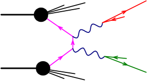
Figure 17: A double Drell-Yan kinematic configuration that can mimic a lepton scattering process.

Thus, when setting up our cuts, we will also consider their effect on the DDY background.

We begin by showing in Figs. 18 and 19 some differential distributions obtained with the basic cuts of eq. (4) for $e^{-}\mu^{-}$ scattering,

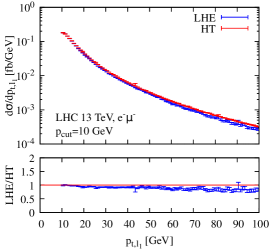
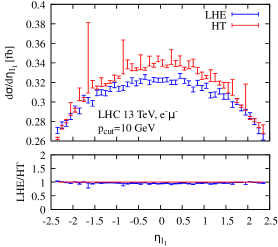
Figure 18: Transverse momentum and rapidity of the electron, for the case of $e^{-}\mu^{-}$ scattering, according to the LHE result (blue) and the HT calculation (red) for $p_{\operatorname{cut}}=10$ GeV.

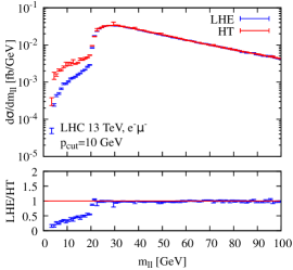
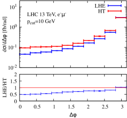
Figure 19: Invariant mass and azimuthal difference of the signal leptons, for the case of $e^{-}\mu^{-}$ scattering, according to the LHE result (blue) and the HT calculation (red) for $p_{\operatorname{cut}}=10$ GeV.

comparing the result of the NLO POWHEG generator at the parton level, i.e. at the level of the Les Houches events file (LHE from now on), with that obtained with the HT method. The most remarkable difference shows up in the distributions of the invariant mass of the pair and their azimuthal distance, in Fig. 19. From the figure, it is apparent that, in the HT calculation, there is a large contribution in the region where the invariant mass of the $e^{-}\mu^{-}$ pair is below twice the transverse momentum cut. The origin of this contribution is easily identified as the production of a back-to-back lepton-antilepton pair with relatively large transverse momentum, with the lepton subsequently radiating a photon, that in turn splits into a second lepton-antilepton pair, as depicted in Fig. 20.

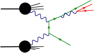
Figure 20: Configurations that contribute to an enhanced production of low mass signal lepton pairs having large transverse momenta in the HT approach.

This mechanism is obviously absent in our NLO+PS calculation, since the $\gamma\gamma$ initial state for our process arises only at the next-to-next to leading order (NNLO) level. The final state has in this case an $l^{-}\ell^{+}\ell^{-}$ low mass system at large transverse momentum, recoiling against a (high transverse momentum) $l^{+}$ lepton, and the $l^{-}\ell^{-}$ system constitutes our signal. This mechanism does not operate at the level of the POWHEG generated Les Houches events, since there no more than three leptons are produced.  It is clear that these events are not the ones we are interested in, especially considering that the DDY process $q\bar{q}\rightarrow l^{+}l^{-}\ell^{+}\ell^{-}$ can generate the same kind of final state, through the mechanism $q\bar{q}\rightarrow\gamma^{\ast}\rightarrow l^{+}\,({l^{-}}^{\ast}\rightarrow l^{-}\,(\gamma^{\ast}\rightarrow\ell^{-}\ell^{+}))$. By requiring $m_{l\ell}>|p_{t}^{(l)}|+|p_{t}^{(\ell)}|$, a condition that we dub “cut A” in the following, we strongly suppress this effect, as shown in Fig. 21.

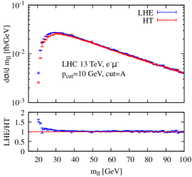
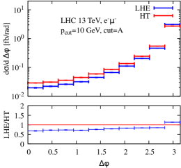
Figure 21: As in figure 19, after imposing cut A.

We see that after cut $A$ is applied, the two calculations are more consistent. We notice, however, that the agreement of the two calculations after cut A is less than perfect, with the POWHEG result overshooting the HT one for small invariant mass and undershooting it for any azimuthal distance away from $\pi$. It is interesting to see that, after shower, the agreement becomes really excellent, as shown in Fig. 22.

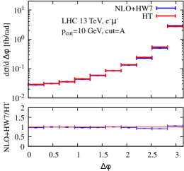
Figure 22: As in figure 19, after imposing cut A and after full shower of the POWHEG result.

This result is not too surprising, since the shower Monte Carlo, by adding also the backward evolution for the incoming quark and photon, captures the most relevant features already present in the HT calculation. In order to reduce the large background from the DDY process $q\bar{q}\rightarrow l^{+}l^{-}\ell^{+}\ell^{-}$ we also impose the following cuts

$$|p_{t}^{l\ell}|/(|p_{t}^{(l)}|+|p_{t}^{(\ell)}|)<0.2\quad\mbox{(cut B) or}\quad 0.1\quad\mbox{(cut C)}\,,$$

that we have found to be particularly effective. Thus the full set of cuts that we have adopted is summarized below:

1. Both signal leptons must have $|\eta|<2.4$, $p_{t}>p_{\rm cut}$.

2. We veto events with extra leptons with $p_{t}>0.9\,$GeV in a cone of radius $r<0.3$.

3. $m_{l\ell}>|p_{t}^{(l)}|+|p_{t}^{(\ell)}|$ (cut A) ,

4. $|p_{t}^{l\ell}|/(|p_{t}^{(l)}|+|p_{t}^{(\ell)}|)<0.2$ (cut B) or  0.1 (cut C) ,

5. If there is another lepton passing cuts i and ii with $p_{t}>3$ GeV the event is vetoed  (cut D).

The cuts (i) and (ii) are always applied. Their combination will be referred to in the tables as “cut T”.

The $e^{-}\mu^{-}$ and $e^{-}\mu^{+}$ cross sections obtained by applying various combinations of cuts are reported in tables 3 and 4. Following our findings on the scale dependence in Section 3.2 we choose as factorization scale the sum of the transverse momentum of all final-state leptons divided by two, ignoring the slight preference for smaller (larger) scale of the $e^{-}\mu^{-}$ ($e^{-}\mu^{+}$) processes.

$e^{-}\mu^{-}$	T	TA	TAB	TABD	TAC	TACD
$\sigma\;\mbox{(fb)},\;p_{\rm cut}=5\,$GeV
LO	$5.789^{+3.343}_{-2.267}$	$5.789^{+3.343}_{-2.267}$	$5.789^{+3.343}_{-2.267}$	$5.789^{+3.343}_{-2.267}$	$5.789^{+3.343}_{-2.267}$	$5.789^{+3.343}_{-2.267}$
NLO	$5.53_{-0.57}$	$4.41_{-1.07}$	$2.21^{+0.59}_{-1.95}$	$1.88^{+0.69}_{-2.08}$	$0.5^{+1.2}_{-2.7}$	$0.4^{+1.2}_{-2.7}$
LHE	$6.300_{-0.762}$	$5.493_{-0.591}$	$3.802_{-0.519}$	$3.580_{-0.544}$	$2.799_{-0.474}$	$2.764_{-0.476}$
NLO+HW7	$6.646$	$5.532$	$3.255$	$2.858$	$1.934$	$1.804$
HT	$6.65$	$5.232$	$3.13$	$2.82$	$2.06$	$1.98$
DDY	$104.$	$28.5$	$4.33$	$1.22$	$1.35$	$0.42$
$\sigma\;\mbox{(fb)},\;p_{\rm cut}=10\,$GeV
LO	$1.432^{+0.734}_{-0.520}$	$1.432^{+0.734}_{-0.520}$	$1.432^{+0.734}_{-0.520}$	$1.432^{+0.734}_{-0.520}$	$1.432^{+0.734}_{-0.520}$	$1.432^{+0.734}_{-0.520}$
NLO	$1.28_{-0.14}$	$1.03^{+0.02}_{-0.24}$	$0.56^{+0.15}_{-0.40}$	$0.31^{+0.23}_{-0.49}$	$0.2^{+0.3}_{-0.5}$	$0.1^{+0.3}_{-0.6}$
LHE	$1.469_{-0.128}$	$1.281_{-0.093}$	$0.920_{-0.129}$	$0.752_{-0.145}$	$0.687_{-0.119}$	$0.652_{-0.121}$
NLO+HW7	$1.488$	$1.262$	$0.847$	$0.664$	$0.563$	$0.496$
HT	$1.53$	$1.234$	$0.80$	$0.63$	$0.55$	$0.50$
DDY	$51.7$	$17.$	$3.02$	$0.47$	$0.95$	$0.2$
$\sigma\;\mbox{(fb)},\;p_{\rm cut}=20\,$GeV
LO	$0.315^{+0.143}_{-0.105}$	$0.315^{+0.143}_{-0.105}$	$0.315^{+0.143}_{-0.105}$	$0.315^{+0.143}_{-0.105}$	$0.315^{+0.143}_{-0.105}$	$0.315^{+0.143}_{-0.105}$
NLO	$0.28_{-0.03}$	$0.22^{+0.01}_{-0.05}$	$0.13^{+0.03}_{-0.08}$	$0.397^{+0.563}_{-1.086}\times 10^{-1}$	$0.570^{+0.502}_{-1.023}\times 10^{-1}$	$0.97^{+6.32}_{-11.81}\times 10^{-2}$
LHE	$0.313_{-0.019}$	$0.270_{-0.016}$	$0.199_{-0.027}$	$0.14^{+0.01}_{-0.03}$	$0.15_{-0.03}$	$0.12_{-0.03}$
NLO+HW7	$0.309$	$0.262$	$0.186$	$0.12$	$0.14$	$0.11$
HT	$0.322$	$0.261$	$0.179$	$0.122$	$0.129$	$0.104$
DDY	$20.$	$8.26$	$2.18$	$0.2$	$0.72$	$0.99\times 10^{-1}$

Table 3: Cross sections in femtobarns for the production of a $e^{-}\mu^{-}$ pair with several combinations of cuts, as detailed in the text, in 13 TeV $pp$ collisions, obtained with: leading order calculation with lepton parton densities; NLO fixed order calculation with lepton parton densities; NLO cross section as generated with POWHEG at the Les Houches event level; full POWHEG result after shower with Herwig7; the HT; and the double Drell-Yan four lepton production $q{\bar{q}}\to\mu\mu^{+}ee^{+}$ computed at leading order. For the LO, NLO and LHE results the quoted uncertainty correspond to the three-point scale variation around the central scale choice.

$e^{-}\mu^{+}$	T	TA	TAB	TABD	TAC	TACD
$\sigma\;\mbox{(fb)},\;p_{\rm cut}=5\,$GeV
LO	$5.737^{+3.316}_{-2.248}$	$5.737^{+3.316}_{-2.248}$	$5.737^{+3.316}_{-2.248}$	$5.737^{+3.316}_{-2.248}$	$5.737^{+3.316}_{-2.248}$	$5.737^{+3.316}_{-2.248}$
NLO	$6.82^{+0.10}_{-0.90}$	$5.70_{-0.54}$	$3.35^{+0.18}_{-1.35}$	$2.95^{+0.31}_{-1.52}$	$1.36^{+0.84}_{-2.24}$	$1.29^{+0.86}_{-2.26}$
LHE	$7.422^{+0.603}_{-1.142}$	$6.595^{+0.424}_{-0.957}$	$4.753^{+0.067}_{-0.572}$	$4.459^{+0.021}_{-0.518}$	$3.483_{-0.395}$	$3.437_{-0.388}$
NLO+HW7	$7.79$	$6.65$	$4.00$	$3.42$	$2.295$	$2.098$
HT	$7.41$	$5.84$	$3.57$	$3.18$	$2.30$	$2.20$
DDY	$105.$	$28.8$	$4.55$	$1.29$	$1.41$	$0.45$
$\sigma\;\mbox{(fb)},\;p_{\rm cut}=10\,$GeV
LO	$1.396^{+0.717}_{-0.507}$	$1.396^{+0.717}_{-0.507}$	$1.396^{+0.717}_{-0.507}$	$1.396^{+0.717}_{-0.507}$	$1.396^{+0.717}_{-0.507}$	$1.396^{+0.717}_{-0.507}$
NLO	$1.56_{-0.15}$	$1.31_{-0.10}$	$0.81^{+0.07}_{-0.27}$	$0.51^{+0.16}_{-0.39}$	$0.37^{+0.20}_{-0.45}$	$0.30^{+0.22}_{-0.47}$
LHE	$1.720^{+0.081}_{-0.216}$	$1.526^{+0.046}_{-0.178}$	$1.130_{-0.105}$	$0.907_{-0.066}$	$0.837_{-0.070}$	$0.790_{-0.063}$
NLO+HW7	$1.76$	$1.53$	$1.05$	$0.78$	$0.67$	$0.57$
HT	$1.67$	$1.365$	$0.895$	$0.680$	$0.600$	$0.537$
DDY	$52.3$	$17.$	$3.21$	$0.51$	$1.01$	$0.2$
$\sigma\;\mbox{(fb)},\;p_{\rm cut}=20\,$GeV
LO	$0.294^{+0.133}_{-0.099}$	$0.294^{+0.133}_{-0.099}$	$0.294^{+0.133}_{-0.099}$	$0.294^{+0.133}_{-0.099}$	$0.294^{+0.133}_{-0.099}$	$0.294^{+0.133}_{-0.099}$
NLO	$0.33_{-0.03}$	$0.27_{-0.03}$	$0.18^{+0.01}_{-0.05}$	$0.674^{+0.437}_{-0.909}\times 10^{-1}$	$0.942^{+0.351}_{-0.813}\times 10^{-1}$	$0.385^{+0.504}_{-1.001}\times 10^{-1}$
LHE	$0.359^{+0.013}_{-0.037}$	$0.315^{+0.006}_{-0.029}$	$0.236_{-0.016}$	$0.16_{-0.01}$	$0.177_{-0.009}$	$0.14_{-0.01}$
NLO+HW7	$0.37$	$0.32$	$0.22$	$0.14$	$0.16$	$0.12$
HT	$0.35$	$0.29$	$0.20$	$0.13$	$0.14$	$0.11$
DDY	$21.$	$8.44$	$2.31$	$0.3$	$0.77$	$0.1$

Table 4: As in table 3 for the $e^{-}\mu^{+}$ process.

First of all, we notice that the NLO+PS and HT results are in good agreement for all combinations of cuts that we considered. We also see that when the simplest cuts are applied, i.e. cut T, all results are in reasonable agreement. On the other hand, as the complexity of the applied cuts increases, the fixed order results departs from the LH-NLO and NLO+PS ones. This is not surprising, and it is a recurring characteristic of fixed order NLO calculations when the events are cut in order to make them more similar to the Born ones. For example, in our case, when we impose the $p_{t}$ balance with cuts B and C, we reduce the size of the real contributions. These are in fact divergent, and are rendered finite by the inclusion of virtual corrections. Asking eventually perfect balance would veto all real events, yielding an infinite negative result. Thus, depending upon the cuts, one can get results that are as small as one pleases, and that can even become negative at fixed order. This effect is quite visible in our table, where, as the cuts become more aggressive, the NLO results decrease and their scale dependence becomes larger, yielding also negative values.

We stress that the LH-NLO result by itself is actually incomplete. For example the transverse momentum of the three hardest leptons is strictly zero at the LH-NLO level. We expect that backward evolution in the shower should lift this constraint, and yield a reasonable transverse momentum distribution for this system, and also reduce further the number of balanced events (i.e. those that pass cut B and C). Therefore we expect that after shower the results should be in better agreement with the HT calculation, that has always the incoming leptons resolved into splitting photons, with the photons in turn being produced in association with a jet (that in the elastic case may consist of a single proton), and in fact this is what we observe in our table. We also show in Fig. 23 the transverse momentum of the signal-leptons pair before and after shower compared with the HT calculation.

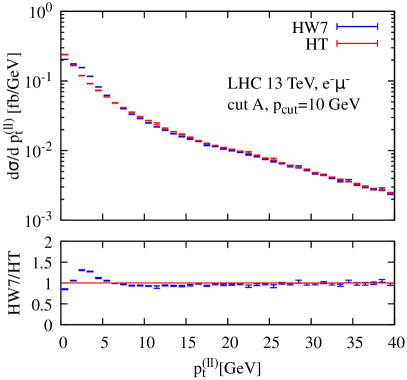
Figure 23: The transverse momentum spectrum of the two-leptons system defined by the two signal leptons, as computed with POWHEG before showering (labeled LHE) (on the left), and after the inclusion of the Herwig7 shower (on the right), both compared to the HT result.

We see the excess in the first bin of the distribution when the shower is absent, that is spread out at larger transverse momenta when the shower is included, yielding a better agreement with the HT result.

As a last comment, we see from the tables 3 and 4 that the combination of cuts $A+B+D$ and $A+C+D$ are most effective in suppressing the DDY background. The effect of the B/C and D cuts is better understood from the following figures. In Fig. 24, on the left panel, we show the electron transverse momentum distribution computed at the NLO+PS level in comparison with the DDY result when only cut A is imposed.

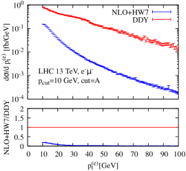
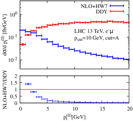
Figure 24: Electron transverse momentum (left) and transverse momentum of the pair (right) for the lepton scattering signal and the double Drell-Yan background (DDY) when cut A is applied.

We see that the lepton spectrum is dominated by the DDY process. On the other hand, we see from the right panel that at low transverse momenta of the lepton pair, the lepton scattering process prevails. The same result when applying the A+B cuts is shown in fig. 25.

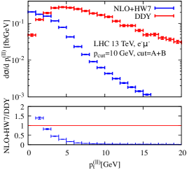
Figure 25: As in fig. 24, for cut A+B.

We see that now the signal in the electron $p_{t}$ emerges from the background at moderate transverse momenta. By adding the further requirement of vetoing other leptons (cut D) we obtain the result displayed in fig. 26.

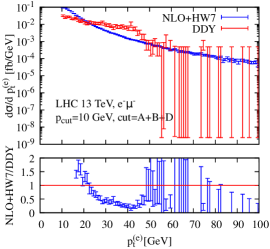
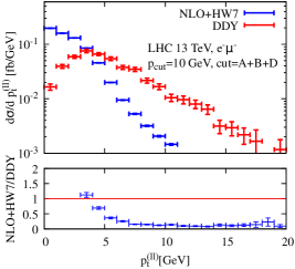
Figure 26: As in fig. 24, for cut A+B+D.

We see that with these cuts the signal prevails over the background as long as the transverse momentum is not too large. This is due to the fact that the DDY process is initiated by one valence quark, while the lepton PDFs are very soft. Some room is left in tightening the cut on the balance, going from B to C, in order to further improve the background rejection, as can be seen in table 3.

Before ending this section, we turn our attention to Fig. 23, where there is a comparison of the transverse momentum distribution of the signal pair obtained at the NLO+PS and HT level. It is quite clear that the modeling of the first few bins is less than satisfactory. We stress that in order to obtain this level of agreement we had to lower the minimum radiation scale of POWHEG from $0.8$ to $0.1$ GeV, and some parameter tuning on the Herwig7 side was also necessary. This, together with similar observations regarding the $\ell/\gamma$-initiated scalar production, reminds us that the current status of the shower generators for $\ell/\gamma$-initiated processes is perhaps not quite mature, and, as the interest in these processes grows, may require further work.

4 Conclusions

In this paper we have used the recently developed photon and lepton PDFs to study the impact of NLO corrections to a number of $\ell/\gamma$-initiated processes and their matching to a parton shower. While at hadron colliders there is considerable experience in matching higher-order calculations to parton showers for pure QCD processes, little is known about this matching in the case of $\ell/\gamma$-induced processes. For this reason, we have first considered two very simple processes, namely the production of a massive scalar particle which couples to incoming photons or leptons. We have found that LO results display a strong scale dependence, which translates into very large uncertainty bands, of the order of ${\cal O}(30\%)$ for $\gamma$- and ${\cal O}(50\%)$ for $\ell$-induced processes. On the other hand, NLO predictions are stable when varying the factorization scale, with missing higher-order uncertainties of the level of 5% for $\gamma$- and 10% for $\ell$-induced production. It is possible to find a choice for the central scale such that the NLO corrections are small, ranging from a few percent to about 20%. For photon induced processes an optimal choice is the mass of the scalar $M_{\Phi}$, while for $\ell$-initiated processes a scale close to $M_{\Phi}/4$ is preferred. We notice in particular that, in the case of $\ell$-initiated processes, the scale choice $M_{\Phi}$ gives rise to large and negative corrections, with the central LO and NLO results differing by a factor 2 and with no overlap between the two uncertainty bands. Thus limits for new physics based upon searches using LO predictions at a scale $M_{\Phi}$ would be overly aggressive, and it would be better to either use a lower scale, or rely on a full NLO calculation.

For photon induced processes we matched the LO and NLO calculations to both Pythia8 and Herwig7 using POWHEG. We find considerable differences between the two predictions at LO, while we obtain a much better agreement after matching to NLO. On the other hand, the two shower Monte Carlo predictions for the very low transverse momentum distribution of the scaler have a very different shape. These features are not relevant for searches of heavy resonances. However, they give an indication that a more accurate tuning of the shower generators is desirable for an accurate modeling of $\gamma$-initiated processes. We note that, while in general Monte Carlos are tuned to data, in the present case the tuning could be performed using predictions obtained with the HT method, since they receive no strong corrections.

The state of the art for $\ell$-initiated processes in shower Monte Carlo programs is even less advanced than for $\gamma$-initiated ones, since they are currently implemented only in a preliminary version of Herwig7. When comparing LO and NLO matched predictions for the transverse momenta of the scalar and of the accompanying jets/leptons, obtained with the optimal scale choices ($M_{\Phi}$ for $\gamma$- and $M_{\Phi}/4$ for $\ell$-initiated processes), we observe a rather flat ratio as long as the transverse momenta are not too small. However, we find considerable differences at small transverse momenta, where NLO corrections have an opposite effect in $\gamma$- and $\ell$-initiated processes. Concerning the $\ell$-initiated processes we find, as expected, that Herwig7 generates small associated hadronic activity, with the transverse momentum spectrum of the leading jet being comparable to the one of the sub-leading lepton. This information is important to enhance the signal to background ratio when looking for these processes. Once available also in Pythia8, it would be certainly interesting to compare Herwig7 and Pythia8 matched predictions also for $\ell$-initiated processes.

We have then considered Standard Model $2\to 2$ lepton-scattering processes, focusing our attention on final states which are not Drell-Yan like, and extending to NLO accuracy the LO results presented in the LUXLep paper. While the NLO calculation is per-se straightforward, care must taken in its implementation in POWHEG, since, starting from NLO, the calculation receives contributions from other electromagnetic sub-processes which involve additional initial- and final-state collinear singularities. In particular, because of the latter, at NLO one needs to impose additional isolation cuts for the final-state signal leptons.

For the lepton-scattering processes we have also performed a calculation in the HT approach, which uses the full hadronic tensor and therefore receives no higher-order QCD corrections. Since the HT calculation misses instead collinear emissions of photons from initial-state leptons, we have estimated these effects by deriving a PDF set where such collinear emissions are switched off. We find that their impact is below one percent for the processes at hand. This implies that one can use the HT calculation as a reference prediction. We note however, that the HT calculation is much more involved than an NLO calculation and that its matching to a parton shower is not straightforward.

As in the case of the production of a scalar particle, we find a considerable reduction in the scale uncertainty when going from LO to NLO. In general, setting the factorization scale to the transverse momentum of the outgoing leptons is a reasonable choice, with slight preferences to lower or higher scales according to the process.

As for the comparison of the HT predictions and the NLO and NLO+PS calculations, we have found the following features. When minimal isolation and acceptance cuts are applied, we find discrepancies between the NLO and the HT result due to a production mechanism that is included in the HT calculation but not in the NLO one, i.e. the production of a back-to-back lepton-antilepton pair with relatively large transverse momentum, followed by the collinear radiation of a photon that in turn splits into a second collinear lepton-antilepton pair. This mechanism enters only at NNLO in the collinear factorization approach. It is clear that these events are not the ones of interest, in particular given that the dominant double Drell-Yan (DDY) background process can generate the same kind of final state. Once one imposes fiducial cuts to suppress this region one finds good agreement between the HT and NLO results.

When considering additional cuts, in order to suppress the large DDY background, the NLO results start departing from the HT one. This is a typical feature of fixed-order NLO calculations in collider physics. As one tightens the cuts in order to make the process look more Born-like, large logarithmically-enhanced negative virtual corrections are exposed that spoil the reliability of fixed-order results. However, once the NLO is matched to a parton shower, after a minimal tuning of the latter, we find very good agreement with the HT result even after stringent cuts. This is also due to the fact that the parton shower generates contributions that are present in the HT calculation and missing in the NLO one. Furthermore, there is certainly room for improvements as the implementation of $\ell$-initiated processes in parton-shower programs is only at its early stage.

As of now, physics with initial photons and leptons have been mostly considered for BSM searches. It would be certainly interesting to experimentally study the lepton-scattering processes, since these are the only SM processes that can probe the lepton content of the proton.

Appendix A The computation of lepton scattering in the hadronic tensor approach

Following the notation of the LUXLep paper, we write the cross section as

$$\sigma = \frac{1}{2S}\int\frac{\mathrm{d}^{4}q_{1}}{(2\pi)^{4}}\frac{1}{q_{1}^{4}}(4\pi)W_{\mu\mu^{\prime}}^{(1)}(P_{1},q_{1})\frac{\mathrm{d}^{4}q_{2}}{(2\pi)^{4}}\frac{1}{q_{2}^{4}}(4\pi)W_{\nu\nu^{\prime}}^{(2)}(P_{2},q_{2})$$ (5)

$$\times T^{\mu\mu^{\prime};\nu\nu^{\prime}}(-q_{1},-q_{2},k_{l})\mathrm{d}\Gamma(2\pi)^{4}\delta\left(-q_{1}-q_{2}-\sum k_{l}\right),$$

where $P_{i}$ ($i=1,2$) are the momenta of the incoming protons, $S=(P_{1}+P_{2})^{2}$, $q_{i}$ are the four momenta of the virtual photons in the DIS convention (i.e. directed towards the protons), $k_{l}$ denote collectively the momenta of the outgoing leptons, $\mathrm{d}\Gamma$ is the corresponding phase space, and  $T^{\mu\mu^{\prime};\nu\nu^{\prime}}$ is the squared matrix element for the production of four leptons initiated by the fusion of two off-shell photons. The process is depicted in Fig. 27,

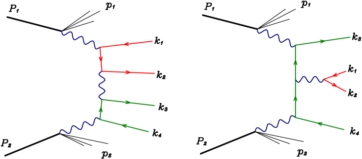
Figure 27: Two sample graphs for the production of two pairs of leptons with different flavours.

where we show two sample Feynman diagrams, involving $t$- and $s$-channel production mechanisms. We computed the phase space by composing nested $2\to 2$ scattering processes, loosely following the approach of Ref. Byckling:1969sx . We thus rewrite eq. (5) in terms of the three-momenta $\vec{p}_{i}$ and masses $\sqrt{s_{i}}$ of the outgoing hadronic systems, as

$$\sigma = \frac{1}{2S}\int\frac{\mathrm{d}s_{1}}{2\pi}\frac{\mathrm{d}s_{2}}{2\pi}\int\frac{\mathrm{d}^{3}p_{1}}{2p_{1}^{0}(2\pi)^{3}}\frac{\mathrm{d}^{3}p_{2}}{2p_{2}^{0}(2\pi)^{3}}\frac{(4\pi)^{2}W_{1}^{\mu\mu^{\prime}}(P_{1},q_{1})W_{2}^{\nu\nu^{\prime}}(P_{2},q_{2})}{Q_{1}^{4}Q_{2}^{4}}$$ (6)

$$\times T_{\mu\mu^{\prime};\nu\nu^{\prime}}(-q_{1},-q_{2},k_{l})\mathrm{d}\Gamma(2\pi)^{4}\delta\left(P_{1}+P_{2}-p_{1}-p_{2}-\sum k_{l}\right),$$

where $p^{0}_{i}=\sqrt{\vec{p}_{i}^{2}+s_{i}}$, and the $s_{i}$ must obey the following constraints

$$s_{i}\geqslant m_{p}^{2},\quad\quad\sqrt{s_{1}}+\sqrt{s_{2}}+\sum m_{l}\leqslant\sqrt{S},$$ (7)

where the $m_{l}$ are the masses of the outgoing leptons. The hadronic tensor $W^{\mu\nu}$ is expressed in terms of the structure functions $F_{1}$ and $F_{2}$ (comprising here also the contribution of the elastic form factors), that in turn are functions of $Q_{i}^{2}=-q_{i}^{2}$ and $x_{\operatorname{bj},i}$. The latter is obtained from the relation

$$s_{i}=Q_{i}^{2}\frac{1-x_{\operatorname{bj},i}}{x_{\operatorname{bj},i}}+m_{p}^{2}.$$ (8)

The elastic component of $F_{1}$ and $F_{2}$ carry a factor of

$$\delta(1-x_{\operatorname{bj},i})=Q_{i}^{2}\,\delta(s_{i}-m_{p}^{2}).$$ (9)

We must compute all four combinations of elastic and inelastic contributions. Thus, when considering the elastic case, we have to replace

$$\int\mathrm{d}s_{i}\rightarrow Q_{i}^{2},$$ (10)

take the $p_{i}$ momentum as having mass $m_{p}$, and write the elastic $F_{i}$ contributions without the $\delta(1-x_{\operatorname{bj},i})$.

We computed $T_{\mu\mu^{\prime};\nu\nu^{\prime}}$ using Madgraph5_aMC@NLO Alwall:2014hca in stand-alone mode. We have generated the process $\gamma\gamma\rightarrow l^{+}l^{-}\ell^{+}\ell^{-}$ for different and identical fermions. Madgraph, by default generates the diagram for given photon polarizations. It does not assume, however, that the incoming momenta are on shell. Thus, we replaced the incoming helicities in the generated formulae with simple Lorentz indices. More specifically, we implemented a routine for the vector-fermion-antifermion vertex that, rather than requiring a helicity in input, requires a Lorentz index. This routine was obtained by modifying the VXXXXX(P,VMASS,NHEL,NSV,VC) Helas Murayama:1992gi routine in such a way that, when called with NHEL = 0, 1, 2, 3, it sets all the VC(3 : 6) components to zero except for the NHEL+3 one, that is set to 1.

The tensor $T$ should vanish when contracted with the momenta corresponding with the two incoming photon, and this served as check for our procedure.

The hadronic tensor is written as

$$W_{\mu\mu^{\prime}}(P,q)=F_{1}\left(-g_{\mu\mu^{\prime}}+\frac{q_{\mu}q_{\mu^{\prime}}}{q^{2}}\right)+\frac{F_{2}}{P\cdot q}\left(P_{\mu}-\frac{P\cdot qq_{\mu}}{q^{2}}\right)\left(P_{\mu^{\prime}}-\frac{P\cdot qq_{\mu^{\prime}}}{q^{2}}\right),$$ (11)

and

$$F_{L}=\left(1+\frac{4x_{\operatorname{bj}}^{2}m_{p}^{2}}{Q^{2}}\right)F_{2}-2x_{\operatorname{bj}}F_{1},$$ (12)

where we have defined $Q^{2}=-q^{2}$. The fitted/calculated values of $F_{2}$ and $F_{L}$ are available in appropriate routines that were developed in the LUX papers. Their value is in part extracted from electro-production data, and in part is calculated in a way that is described there in great detail.

The phase space in eq. (5) requires great care, since it is logarithmically singular in several regions, the logarithmic singularities being regulated by the proton and the lepton masses. Following Ref. Byckling:1969sx , we factorize the phase space as a sequence of nested two-body components. Our main integration variables are thus the $s$-channel and $t$-channel invariants of these two-body components, that are chosen in such a way that the logarithmically enhanced regions are adequately sampled.

A.1 Basic $2\rightarrow 2$ formulae

The basic $p_{1}\,p_{2}\rightarrow p_{3}\,p_{4}$ cross section formula for generic masses is

$$\mathrm{d}\sigma = \frac{|\mathcal{M}|^{2}}{4\sqrt{(p_{1}\cdot p_{2})^{2}-m_{1}^{2}m_{2}^{2}}}\mathrm{d}\Phi_{2}\,,$$

$$\mathrm{d}\Phi_{2} = (2\pi)^{4}\delta^{4}(q-p_{3}-p_{4})\frac{\mathrm{d}^{3}p_{3}}{2p_{3}^{0}(2\pi)^{3}}\frac{\mathrm{d}^{4}p_{4}}{(2\pi)^{4}}2\pi\delta(p_{4}^{2}-m_{4}^{2})$$

$$= \frac{1}{32\pi^{2}}\frac{2\underline{p}_{3}}{q}\mathrm{d}\cos\theta\,,\mathrm{d}\phi,$$

where $q=p_{1}+p_{2}$ and $s=q^{2}$. We denote as $\underline{p}=\sqrt{\vec{p}^{2}}$, that in the above formula is taken in the CM system of $q$. We have

$$p_{3}^{0}=\frac{s+m_{3}^{2}-m_{4}^{2}}{2\sqrt{s}}\,.$$ (13)

We can introduce

$$t=(p_{1}-p_{3})^{2}=m_{1}^{2}+m_{3}^{2}-2p_{1}^{0}p_{3}^{0}+2\underline{p}_{1}\underline{p}_{3}\cos\theta\,,$$ (14)

and

$$u=(p_{2}-p_{3})^{2}=m_{2}^{2}+m_{3}^{2}-2p^{0}_{2}p_{3}^{0}-2\underline{p}_{1}\underline{p}_{3}\cos\theta\,,$$ (15)

so we can also write

$$\mathrm{d}\sigma = \frac{|\mathcal{M}|^{2}}{4\sqrt{(p_{1}\cdot p_{2})^{2}-m_{1}^{2}m_{2}^{2}}}\left[\frac{1}{32\pi^{2}}\frac{2\underline{p}_{3}}{q}\frac{1}{2\underline{p}_{1}\underline{p}_{3}}\mathrm{d}t\mathrm{d}\phi\right]$$

$$= \frac{|\mathcal{M}|^{2}}{4\sqrt{(p_{1}\cdot p_{2})^{2}-m_{1}^{2}m_{2}^{2}}}\left[\frac{1}{16\pi}\frac{1}{\sqrt{s}}\frac{1}{\underline{p}_{1}}\mathrm{d}t\frac{\mathrm{d}\phi}{2\pi}\right]\,.$$

As a further simplification we use the identity

$$(p_{1}\cdot p_{2})^{2}-m_{1}^{2}m_{2}^{2}=s\,\underline{p}_{1}^{2},$$ (16)

so we obtain finally

$$\mathrm{d}\sigma=\frac{|\mathcal{M}|^{2}}{64\pi}\frac{1}{s}\frac{1}{\underline{p}_{1}^{2}}\mathrm{d}t\frac{\mathrm{d}\phi}{2\pi}\,,$$ (17)

where the limits for $t$ are

$$m_{1}^{2}+m_{3}^{2}-2p_{1}^{0}p_{3}^{0}+2\underline{p}_{1}\underline{p}_{3}>t>m_{1}^{2}+m_{3}^{2}-2p_{1}^{0}p_{3}^{0}-2\underline{p}_{1}\underline{p}_{3}\,.$$ (18)

A.2 Composition of the phase space

We describe here for simplicity the production of two pairs of leptons of different flavour, as in Fig. 27. We assume that our signal leptons are those labeled as 2-3. The phase space is decomposed according to the following sequence:

$$P_{1}+P_{2} \rightarrow p_{1}+(k_{1}+k_{2}+k_{3}+k_{4}+p_{2}),$$

$$(P_{1}-p_{1})+P_{2} \rightarrow (k_{1}+k_{2}+k_{3}+k_{4})+p_{2},$$

$$(P_{1}-p_{1})+(P_{2}-p_{2}) \rightarrow k_{1}+(k_{2}+k_{3}+k_{4}),$$

$$(P_{1}-p_{1}-k_{1})+(P_{2}-p_{2}) \rightarrow (k_{2}+k_{3})+k_{4},$$

$$(P_{1}-p_{1}-k_{1})+(P_{2}-p_{2}-k_{4}) \rightarrow k_{2}+k_{3},$$

where the momenta in bracket denote a massive system, with an appropriate bound for its mass. For example, for the first line of the equation, the minimal mass of $p_{1}$ is $m_{p}$, and its maximum is $\sqrt{S}-(m_{1}+m_{2}+m_{3}+m_{4}+m_{p})$; the minimal mass of the $(k_{1}+k_{2}+k_{3}+k_{4}+p_{2})$ system if $m_{1}+m_{2}+m_{3}+m_{4}+m_{p}$, and its maximum is $\sqrt{S}-m_{p}$.

The structure functions have an elastic and inelastic component. In the elastic case, $p_{i}$ has fixed invariant mass equal to $m_{p}$. Thus, all components, elastic-elastic, inelastic-elastic, elastic-inelastic and inelastic-inelastic must be generated independently. As a further point, the procedure outlined above is adequate for the sampling of the $t$-channel singularities if lepton 1 is produced mainly along the $P_{1}$ direction, and lepton 4 along the $P_{2}$ one, a region that we here dub region $a$. In order to perform an adequate sampling, we define an enhancement factor that singles out region $a$

$$f_{a}=\frac{1}{(P_{1}-p_{1}-k_{1})^{2}(P_{2}-p_{2}-k_{4})^{2}},$$ (19)

and one that singles out the complementary region $b$ where 1 is produced along the $P_{2}$ direction and 4 along $P_{1}$

$$f_{b}=\frac{1}{(P_{1}-p_{1}-k_{4})^{2}(P_{2}-p_{2}-k_{1})^{2}}.$$ (20)

We then multiply the cross section by the factor

$$\frac{f_{a}}{f_{a}+f_{b}},$$ (21)

thus suppressing region $b$. The contribution of region $b$ is obtained by generating the phase space with the role of the two flavours exchanged, providing again the similar suppression factor.

Several other regions of singularity are present, that however do not contribute significantly to our signal. In order to speed up convergence for the distributions that we are interested in, we suppress these regions with adequate suppression factors. The generated events have this suppression factor removed, so that one obtains the exact cross section, but with less dense sampling in the uninteresting regions. These regions are

• The region when the $k_{1},k_{2}$ and/or the $k_{3},k_{4}$ systems have small masses. These regions do not generate isolated leptons with the appropriate charge. We thus suppress these regions with a factor proportional to these masses.

• The region where the signal leptons $k_{3}$ and $k_{4}$ are not in a reasonable acceptance range. In particular, they must have a sizeable transverse momentum, and their pseudorapidity should be within acceptance. The suppression factors that we adopt are

  $$\frac{k_{T,2}^{2}}{k_{T,2}^{2}+k^{2}_{T,\operatorname{cut}}}\times\left(\frac{y_{\operatorname{cut}}}{|y_{3}|+y_{\operatorname{cut}}}\right)^{2}\times\left(\frac{m_{12}^{2}}{m_{12}^{2}+m^{2}_{\operatorname{cut}}}\right)^{2}\times(2\rightarrow 3,1\rightarrow 4).$$ (22)

Appendix B Mass corrections in the POWHEG computation

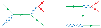
Figure 28: Diagrams that lead to a final-state collinear singularity.

In this appendix we detail how we include mass effects to cure the collinear divergence arising from squaring the photon splitting diagrams depicted in Fig. 28. First, let us remark that this problem does not show up in a complete massive computation. However, such a computation cannot be performed in the collinear factorization approach. Second, these contributions have as underlying Born the Compton process; thus, in our treatment, they contribute only to the remnant cross section, as discussed in Sec. 3.1. This means that we have to deal only with the real matrix elements, with no need to modify subtraction counterterms.

We proceed as follows. We start by computing the square of the two diagrams in Fig. 28 assuming the green fermion line, associated to lepton $l$, as massless and the red one, associated to lepton $\ell$, as massive. Observe that in the limit for a vanishing mass the resulting function, that we dub $f_{c}(p;m_{\ell})$, smoothly approaches the massless squared matrix element that exhibits a collinear final-state singularity. Next, we look for all possible $\ell{\bar{\ell}}$ pairs in the final state; there are two in the case of identical leptons and just one otherwise. For each pair, we let the momenta of these two massless leptons acquire mass by retaining their 3-momentum while correcting their energy. The resulting real event has a slightly increased centre of mass energy. In formulae, writing the original set of momenta $p_{i}$ in the partonic centre of mass defined by

$$p_{1,2}=\frac{\sqrt{s}}{2}(1,0,0,\pm 1),$$ (23)

where $\sqrt{s}$ is the partonic centre of mass energy, the set of massive momenta is given by

$$p^{\prime}_{1,2}=\frac{\sqrt{s^{\prime}}}{2}(1,0,0,\pm 1),\quad p^{\prime}_{3,4}=\left(p_{3,4}^{0}\sqrt{1+\left(\frac{m_{\ell}}{p_{3,4}^{0}}\right)^{2}},\mathbf{p}_{3,4}\right),\quad p^{\prime}_{5}=p_{5}$$ (24)

assuming that the $\ell{\bar{\ell}}$ pair has momenta $p_{3}$ and $p_{4}$ and $\sqrt{s^{\prime}}=p_{3}^{\prime,0}+p_{4}^{\prime,0}+p_{5}^{\prime,0}$. We correct the real matrix element by adding the quantity

$$\Delta_{c}=f_{c}(p^{\prime};m_{\ell})-f_{c}(p;0).$$ (25)

In the case of identical leptons, we add the correction factor $\Delta_{c}$ for each of the two pairs found, and divide by the appropriate symmetry factor.

For the sake of completeness, we report here the explicit expression of the correction function $f_{c}$ assuming that the collinear leptonic pair has momenta $p_{3}$ and $p_{4}$ and that $p_{2}$ is the incoming photon:

$$f_{c}(p;m_{\ell})=-\frac{4}{s_{12}s_{25}(2m_{\ell}^{2}+s_{34})^{2}}(A+2Bm_{\ell}^{2})\,,$$ (26)

in terms of the invariants $s_{ij}=2p_{i}\cdot p_{j}$ and the coefficients

$$\begin{split}A&=s_{12}s_{14}s_{23}+s_{14}s_{15}s_{23}+s_{12}s_{13}s_{24}+s_{13}s_{15}s_{24}+s_{12}s_{14}s_{35}+2s_{14}s_{15}s_{35}-2s_{13}s_{14}s_{25}\\ &+s_{15}s_{24}s_{35}+s_{14}s_{25}s_{35}+s_{24}s_{25}s_{35}+s_{12}s_{13}s_{45}+s_{15}s_{23}s_{45}+2s_{13}s_{15}s_{45}-2s_{12}s_{35}s_{45}\\ &+s_{13}s_{25}s_{45}+s_{23}s_{25}s_{45}\,,\\ B&=(s_{12}+s_{15})^{2}+(s_{15}+s_{25})^{2}\,.\end{split}$$ (27)

References

- (1) A. Manohar, P. Nason, G. P. Salam and G. Zanderighi, How bright is the proton? A precise determination of the photon parton distribution function, Phys. Rev. Lett. 117 (2016) 242002, [1607.04266].
- (2) A. V. Manohar, P. Nason, G. P. Salam and G. Zanderighi, The Photon Content of the Proton, JHEP 12 (2017) 046, [1708.01256].
- (3) L. Buonocore, U. Haisch, P. Nason, F. Tramontano and G. Zanderighi, Lepton-Quark Collisions at the Large Hadron Collider, Phys. Rev. Lett. 125 (2020) 231804, [2005.06475].
- (4) M. Drees and D. Zeppenfeld, Production of Supersymmetric Particles in Elastic Collisions, Phys. Rev. D39 (1989) 2536.
- (5) A. Greljo and N. Selimovic, Lepton-Quark Fusion at Hadron Colliders, precisely, JHEP 03 (2021) 279, [2012.02092].
- (6) P. Nason, A New method for combining NLO QCD with shower Monte Carlo algorithms, JHEP 11 (2004) 040, [hep-ph/0409146].
- (7) S. Frixione, P. Nason and C. Oleari, Matching NLO QCD computations with Parton Shower simulations: the POWHEG method, JHEP 11 (2007) 070, [0709.2092].
- (8) S. Alioli, P. Nason, C. Oleari and E. Re, A general framework for implementing NLO calculations in shower Monte Carlo programs: the POWHEG BOX, JHEP 06 (2010) 043, [1002.2581].
- (9) T. Sjöstrand, S. Ask, J. R. Christiansen, R. Corke, N. Desai, P. Ilten, S. Mrenna, S. Prestel, C. O. Rasmussen and P. Z. Skands, An Introduction to PYTHIA 8.2, Comput. Phys. Commun. 191 (2015) 159–177, [1410.3012].
- (10) J. Bellm et al., Herwig 7.2 release note, Eur. Phys. J. C 80 (2020) 452, [1912.06509].
- (11) L. A. Harland-Lang, Physics with Leptons and Photons at the LHC, 2101.04127.
- (12) L. Buonocore, P. Nason, F. Tramontano and G. Zanderighi, Leptons in the proton, JHEP 08 (2020) 019, [2005.06477].
- (13) A. Buckley, J. Ferrando, S. Lloyd, K. Nordström, B. Page, M. Rüfenacht, M. Schönherr and G. Watt, LHAPDF6: parton density access in the LHC precision era, Eur. Phys. J. C75 (2015) 132, [1412.7420].
- (14) P. Richardson, R. R. Sadykov, A. A. Sapronov, M. H. Seymour and P. Z. Skands, QCD parton showers and NLO EW corrections to Drell-Yan, JHEP 06 (2012) 090, [1011.5444].
- (15) B. Cabouat and T. Sjöstrand, Some Dipole Shower Studies, Eur. Phys. J. C 78 (2018) 226, [1710.00391].
- (16) G. P. Salam and J. Rojo, A Higher Order Perturbative Parton Evolution Toolkit (HOPPET), Comput. Phys. Commun. 180 (2009) 120–156, [0804.3755].
- (17) T. Melia, P. Nason, R. Rontsch and G. Zanderighi, plus dijet production in the POWHEGBOX, Eur. Phys. J. C 71 (2011) 1670, [1102.4846].
- (18) S. Alioli, K. Hamilton, P. Nason, C. Oleari and E. Re, Jet pair production in POWHEG, JHEP 04 (2011) 081, [1012.3380].
- (19) L. A. Harland-Lang, M. Tasevsky, V. A. Khoze and M. G. Ryskin, A new approach to modelling elastic and inelastic photon-initiated production at the LHC: SuperChic 4, Eur. Phys. J. C 80 (2020) 925, [2007.12704].
- (20) E. Byckling and K. Kajantie, N-particle phase space in terms of invariant momentum transfers, Nucl. Phys. B 9 (1969) 568–576.
- (21) J. Alwall, R. Frederix, S. Frixione, V. Hirschi, F. Maltoni, O. Mattelaer, H. S. Shao, T. Stelzer, P. Torrielli and M. Zaro, The automated computation of tree-level and next-to-leading order differential cross sections, and their matching to parton shower simulations, JHEP 07 (2014) 079, [1405.0301].
- (22) H. Murayama, I. Watanabe and K. Hagiwara, HELAS: HELicity amplitude subroutines for Feynman diagram evaluations, .