Roller-Coaster in a Flatland: Magnetoresistivity in Eu-intercalated Graphite
Abstract
Novel phenomena in magnetically-intercalated graphite has been a subject of much research, pioneered and promoted by M. S. and G. Dresselhaus and many others in the 1980s. Among the most enigmatic findings of that era was a dramatic, roller-coaster-like behavior of the magnetoresistivity in EuC6 compound, in which magnetic Eu2+ ions form a triangular lattice that is commensurate to graphite honeycomb planes. In this study, we provide a long-awaited microscopic explanation of this behavior, demonstrating that the resistivity of EuC6 is dominated by spin excitations in Eu-planes and their highly nontrivial evolution with the magnetic field. Together with our theoretical analysis, the present study showcases the power of the synthetic 2D materials as a source of potentially significant insights into the nature of exotic spin excitations.
I Introduction
The two-dimensional (2D) world of Flatland, a mathematical abstraction and a cultural reference [1], has, arguably, received its ultimate physical realization in the form of graphene [2, 3], whose unique properties [4] have ushered in a new era of making artificial heterostructures via a Lego-like [5] assembly of layered materials. Together with the research in the twisted bi- and -layer graphene [6], the fledging field of van der Waals magnets holds a lot of promise in opening new horizons for the fundamental studies and applications along the path of using this technology [7, 8, 9, 10, 11].
Historically, a more traditional, if not ancient [12], way of achieving similar goals of synthesizing materials with novel properties from a stack of carbon layers and various elements and compounds has relied on the process of intercalation, suggesting another cultural metaphor [13]. The research in graphite intercalation compounds (GICs) has attracted significant attention in the past, with the evolution of such studies and understanding of these materials outlined in several books and, specifically, in the reviews by M. S. and G. Dresselhaus, whose efforts contributed to much of the progress in this area, see Refs. [14, 15, 16, 17].
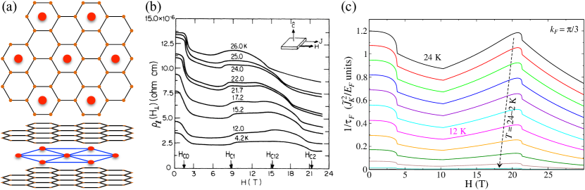
Of the fundamental footprint of this research, it is the magnetically-intercalated compounds that have produced the most intriguing phenomena [16]. The case of EuC6, made of alternating honeycomb layers of carbon and triangular-lattice layers of Eu ions, shown schematically in Fig. 1(a), particularly stands out. A highly dramatic, roller-coaster-like dependence of the in-plane resistivity on a magnetic field, reproduced from Ref. [18] in Fig. 1(b), is clearly indicative of an intricately intertwined magnetic and electronic degrees of freedom of this material. Incidentally, EuC6 is also the first magnet to exhibit the fabled -magnetization plateau [19] and was inspirational for an understanding of this state [20].
The pioneering studies of EuC6 [21, 22, 23, 18] have analyzed and successfully identified key exchange terms of the triangular-lattice spin- model Hamiltonian of the localized orbitals of Eu2+ ions that are necessary to understand the field-induced phases and the concomitant magnetization data [19]. However, while yielding a reasonable estimate of the Kondo coupling, the sole attempt to explain magnetoresistivity itself [24] has provided a largely unsuccessful modeling of it via a crude consideration of the spin-scattering of electrons and suggested a rather relic backflow mechanism to explain the -dependence of the resistivity.
Thus, it is fair to say that, by and large and to the best of our knowledge, there exists no proper explanation of the key resistivity results observed in EuC6, shown in Fig. 1(b). Furthermore, the refocusing of the research of the 1980s and 1990s on correlated systems and high-temperature superconductivity has left these striking results in their enigmatic state.
In this work, we provide a microscopic theory of the magnetoresistivity of EuC6 and demonstrate that its highly nontrivial evolution with the magnetic field can be fully accounted for by the scattering off the spin excitations in Eu-planes. Figure 1(c) demonstrates representative results of our theory, which capture most of the qualitative and quantitative features of the experimental data in Fig. 1(b), with the details of the theory provided below. Our effort brings together research in the magnetically-intercalated graphite compounds with that in the novel graphite-derived artificial magnetic materials [8, 17, 25].
More broadly, we would also like to highlight that there is a number of conducting magnetic materials that exhibit a highly non-monotonic magnetoresistivity [26, 27, 28, 29], showing that such measurements can serve as a very sensitive probe of the field-induced phase transitions. However, most theoretical explanations, if any, are limited to an associative construction of phenomenological spin models to match the number of phase transitions and broad trends in magnetization [29], without any attempt to explicate scattering mechanisms and calculate resistivity. In that respect, our present study is also the one that accomplishes precisely this goal: a fully microscopic calculation of the resistivity throughout all the phases in the phase diagram of the underlying spin model. We anticipate our results not only be inspirational for the broader research in metallic magnets, but also to provide the technical guidance for similar studies.
We outline, in broad strokes, our approach and results. We build on the achievements of the prior work on EuC6 [21, 22, 23, 18] and reanalyze phenomenological constraints on the triangular-lattice spin- model of Eu2+ layers. In this analysis, we also use more recent experimental insights into the magnetic ground state of EuC6 [30] and density-functional theory of its electronic structure [31].
Thus, we establish bounds on the exchange parameters as related to the phenomenology of different magnetic phases of EuC6, examine ranges of parameters that make transitions between the phases first-order, and formulate a minimal model to describe EuC6. We proceed by constructing the spin-wave theory for all the field-induced phases of that model. Although a numerical procedure is generally needed to obtain magnon eigenenergies, the approach leading to it, as well as the results for some of the phases, are fully analytical.
While the Kondo coupling between conducting electronic states and Eu2+ spins is fully local, the matrix elements of electron scattering on magnons have a nontrivial form, owing to the internal structure of quasiparticle eigenstates in different phases. This structure leads, among other things, to the non-spin-flip scattering processes in the non-collinear phases. We articulate that these matrix elements are essential for a consistent calculation of the transport scattering rate. The expression for the latter, given in a concise form, is derived using Boltzmann formalism, which we revisit for both spin-flip and non-spin-flip channels, providing a thorough derivation of the relaxation-time approximation in the process.
The temperature-dependence of the resistivity anticipated from our theory is discussed for all field-induced phases. Significantly, the zero-field results of our theory demonstrate an analogue of the phonon-dominated resistivity behavior, but due to scattering off the acoustic magnons of the 120 state, with a 2D equivalent of the Bloch-Grüneisen low-temperature asymptote of and the high-temperature Ohm’s law, . Given the extent of the magnon bandwidth, the nearly linear trend of observed in Ref. [24] above 8 K is shown to be well within the onset of the Ohm’s regime.
The resistivity calculations are performed at experimentally relevant temperatures for various parameters of the minimal model to demonstrate qualitative trends and for a specific set of parameters that best describes EuC6. We also investigate the dependence of our results on the filling fraction of electronic bands, encoded in the Fermi momentum , and conclude that the relatively smaller values of provide a better correspondence to the EuC6 phenomenology, inviting more research into a verification of its electronic properties. Other intriguing features of the resistivity for the larger values of , potentially controllable by doping, are also discussed.
Altogether, the results of our model for the transport relaxation rate, offered in Fig. 1(c) for a representative , show a striking similarity to the experimental data in Fig. 1(b), with the possible origin of the discrepancies at higher field discussed below. Our theory implicitly contains the field-dependence via that of the magnon spectra and scattering matrix elements, which, in turn, depend on the spin arrangement in each of the field-induced phases. It also properly accounts for the effect of the thermal population of magnetic scatterers on the resistivity. One of the qualitative messages of our study is the importance of the non-spin-flip channel of the scattering, which is present in the phases with the non-collinear spin configurations, but is absent for the collinear ones. This effect explains the weaker scattering and lower resistivity in the -magnetization plateau and fully polarized phases.
The general picture that emerges from our analysis is that of the resistivity as a very informative probe of not only field-induced phase transitions, but also of the elementary spin excitations in these phases. The provided thorough theoretical analysis of the iconic two-dimensional triangular-lattice antiferromagnet coupled to conduction electrons showcases a largely untapped power of the synthetic 2D materials as a source of potentially significant insights into the nature of exotic spin excitations. Our approach and findings can be applied, for example, to the electron scattering by the fractionalized spinons of the Kitaev spin liquid [32, 33] and to the other magnetically-intercalated systems such as chalcogenides [34, 35, 36].
The paper is organized as follows. Section II.1 discusses electronic structure of EuC6 and the approximate values of the Fermi momenta. Section II.2 gives an overview of the phenomenologically-motivated spin model of EuC6, its classical ground states and critical fields, and parameters of the minimal model. Details on the first-order transitions are delegated to Appendix A. Spin excitations of the model for all field-induced phases are discussed in Section III, which provides details of the spin-wave formalism and results for representative magnon eigenenergies and the eigenfunctions. The fully analytical results for the polarized, 120, and plateau phases are given in Appendix B.
The Kondo coupling and its estimate, as well as resistivity and some qualitative insight into it, are discussed in Section IV. This consideration relies, not in a small way, on a detailed derivation of the relaxation rates for the spin-flip and non-spin-flip channels from the Boltzmann formalism, provided in Appendix C, which also discusses possible limitations of this approach and potential new phenomena at large values of . The temperature-dependence of magnetoresistivity, results for various values of the key model parameters and Fermi momentum, and an outlook on the possible future extensions are given in Section V. We provide a summary in Section VI.
II Phenomenology and modeling
II.1 Electronic structure of EuC6
The electronic structure of Eu-intercalated graphite EuC6 has been investigated experimentally and theoretically in the mid-90s of the last century [31], with the summary of these efforts given in Ref. [17].
Structurally, EuC6 is the so-called stage-I intercalated compound, meaning that the Eu layers alternate with that of carbon. Viewed from a graphite layer, the rare-earth atoms are located on top of the centers of the graphite hexagons and form a superstructure as is illustrated in Fig. 1(a). The material is characterized by the so-called stacking (space group ), in which Eu atoms form a hexagonal closed packed structure with alternating positions and between consecutive layers, while carbons follow the stacking [37, 38, 30]. This arrangement of carbon sheets is different from the , or Bernal, stacking of the graphite.
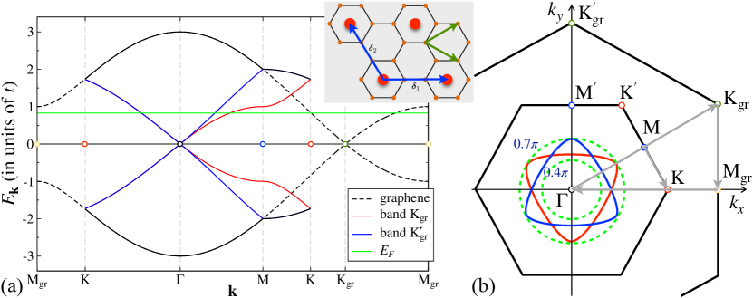
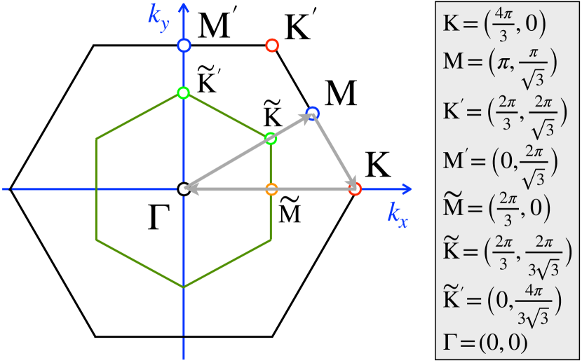
As a result, the principal unit associated with the Eu-based triangular lattice can be seen as containing one Eu and six carbon atoms, while the structural unit cell contains two Eu atoms and twelve carbons. As is shown in Fig. 2(b), the two-dimensional (2D) Brillouin zone (BZ) of the triangular Eu lattice is three times smaller than that of the graphene. The lattice constants of the triangular Eu lattice and that of the honeycomb graphene lattice are related as , see Fig. 2.
The key features of the electronic band structure of EuC6 can be understood within the “rigid-band” approximation, see Ch. 5 of Ref. [17]. One assumes that the band structure of the graphene layer is not changed by the Eu intercalation, with the latter resulting only in a partial filling of the graphene bands up to a Fermi energy , illustrated in Fig. 2(a) by a horizontal line.
Upon folding onto the Eu-based Brillouin zone, the Dirac bands are mapped from the proximities of the Kgr and K points of the graphene Brillouin zone onto the neighborhood of the point, see Fig. 2. These bands are equivalent up to a rotation, with a representative constant-energy cut demonstrating characteristic “flower-petal” Fermi surfaces originating from the trigonal symmetry of the graphene lattice, see Fig. 2(b). These two bands from the two valleys at Kgr and K are the ones being filled away from the charge-neutrality point by the doping provided by the intercalated Eu.
To estimate the size of the Fermi surfaces produced by doping, one can approximate them as circles with a radius , neglecting their trigonal warping. Naturally, the Fermi momentum is determined by the 2D density of electrons donated to a graphene sheet by the Eu layer. Taking into account band (valley) and spin degeneracy factors yields [17]. The nominal valence state of Eu is Eu2+. Assuming that all 2/Eu go into the conduction bands and using the 2D volume of the Eu unit cell , one obtains . The same result can be obtained by matching the area (2D volume) of the fully occupied, doubly-degenerate triangular-lattice Brillouin zone of the Eu lattice, , with the four-fold degenerate (valleyspin) Fermi circle of radius . Altogether, the Fermi surface in EuC6, estimated within this approach, is expected to be large.
The detailed calculations of electronic structure of EuC6 in Ref. [31] feature the band-structure that is not unlike the rigid-band picture in Fig. 2(a), with the bands that are crossing the Fermi level clearly reminiscent of the folded graphene bands. However, two key differences are a significantly lower doping of the carbon -orbitals, which accounts for about per Eu2+, and the rest of electrons filling up the Eu-derived -hybrid band, with the latter absent in the rigid-band description [31, 17]. These findings are also supported by the angle-resolved photoemission studies of stage-I EuC6 and stage-II EuC12 materials, reported in Ref. [31].
The most direct implication of the first result for our analysis of the Fermi surfaces is the four times smaller density of donated electrons, which straightforwardly translates into the two times smaller Fermi momentum in the graphene conduction bands, . We also estimate the Fermi momenta of the “true,” trigonally warped Fermi surfaces from the band structure in Ref. [31] as and , in a qualitative agreement with the estimate of above. Our choice of the representative (in units of eV [4]) in Fig. 2(a) and of the resultant Fermi surfaces in Fig. 2(b) is made to match the Fermi momenta from Ref. [31], which, in turn, should approximately correspond to the filling of the bands.
The other shortcoming of the rigid-band approximation is the omission of the Eu-derived partially filled -hybrid band [31, 17]. It was also argued that the hybridization of the Eu -orbitals and graphene -orbitals is responsible for the mediation of the strong Kondo interaction between the localized -orbital spins of Eu and conduction -orbital electrons of graphite, estimated at eV [24]. This key element of our study is described in Sec. IV.1.
In our analytical treatment of the scattering rate in Sec. IV.2 and Appendix C, we are motivated by the analysis and discussion provided in this Section and approximate the relevant electronic degrees of freedom of EuC6 by the two degenerate bands with the circular Fermi surfaces of radius centered around point. We treat as a parameter and show how the key features of the calculated magnetoresistivity evolve with it, see Sec. V. We expect the renewed interest in the problem to result in a convergence of the band-structure calculations with the experimental data regarding the relevant electronic structure and parameters of EuC6 and other GICs.
II.2 Spin model and parameters
It has been proposed in Refs. [18, 21, 22, 23] that the minimal model that describes phenomenology of the magnetism in EuC6 is the triangular-lattice model
| (1) |
where denote the (next-)nearest-neighbor bonds with the corresponding exchanges and in the Zeeman term. A crucial ingredient of this model is the biquadratic term. While may be small compared to the exchanges, it is important because of the amplification factor.
It was argued in Refs. [18, 21, 22, 23] that this minimal model would not be complete without the ring-exchange term, which is discussed below in some more detail. While the biquadratic and ring-exchange terms play similar role in stabilizing the up-up-down (UUD or plateau) state in a wide range of fields, our analysis of the EuC6 phenomenology provided below points to the values of the ring exchange that are secondary to , differing from the values advocated in Refs. [18, 21]. However, given a close similarity of their effects, this variation is likely inconsequential and amounts to a different parametrization of such effects within an effective model. In the spin-wave consideration that follows, we will ignore the ring-exchange term entirely, citing cumbersomeness of its treatment.
Another difference of our model from the consideration of Refs. [18, 21, 22, 23] is that the exchange terms in (1) are taken as Heisenberg, not . This makes no difference for the classical phase diagram in the in-plane field, which was simulated using classical Monte-Carlo in Ref. [18] in the limit. However, the actual anisotropy in EuC6 is unlikely to exceed 10%, as is evidenced by the very similar saturation fields in the in-plane and out-of-plane magnetization and by the nearly isotropic -factors [18], justifying our choice of the isotropic limit of the model.
II.2.1 Classical ground states
In this work, we focus exclusively on the field orientation that is in the plane of Eu2+ ions, see Fig. 3. While for the isotropic approximation that we choose in model (1) the direction of the field is irrelevant, the phenomenology that follows identifies with that of the in-plane field data for EuC6, which exhibits a weak easy-plane () anisotropy [21]. The out-of-plane field direction in this latter case yields a different, and much simpler, magnetization and ground state evolution [39].
Triangular-lattice antiferromagnets host a rather astonishing variety of the unconventional field-induced phases, see Refs. [40, 41, 42]. As we have noted above, EuC6 was the first material in which the best-known of such unconventional phases, the UUD magnetization plateau state, has been identified [19].
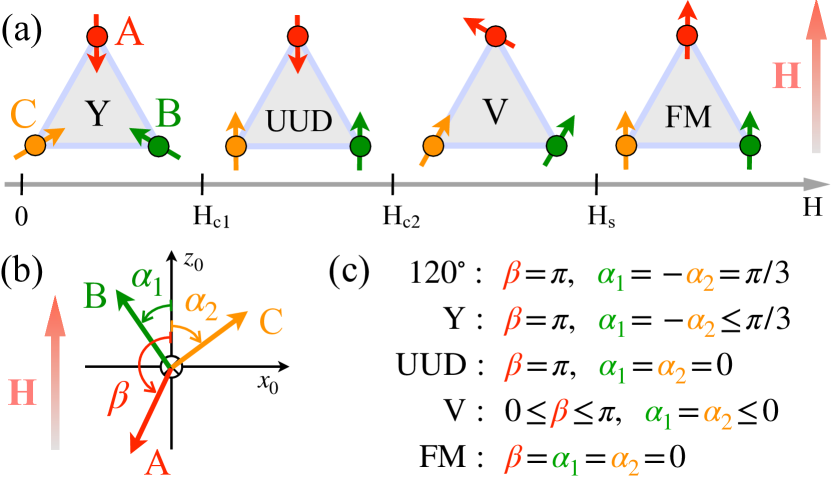
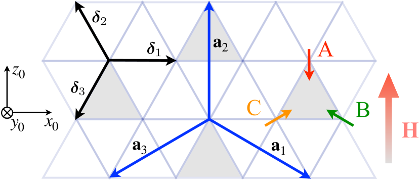
For the model (1), the field-evolution of the classical ground states is known from the earlier works [20, 41, 21] with the schematics of the evolution of magnetic order with the field shown in Fig. 4(a). At , spins assume a 120 configuration that was confirmed for EuC6 by the muon-spin spectroscopy [30]. A finite field continuously deforms it into the so-called Y-structure followed by a transition to the UUD (plateau) state at . The spin angles and the field direction are shown in Fig. 4(b) and (c). The higher field induces a transition from the UUD phase to the V phase at and to the fully polarized FM phase at the saturation field . It is worth noting that in all ordered phases, spin configurations are coplanar and belong to the three-sublattice structure with the same unit cell, see Fig. 3 and Fig. 4.
In the earlier studies of EuC6 [18, 21, 22, 23], the minimal model (1) was also augmented by the ring-exchange term
| (2) |
where and spins belong to the elementary nearest-neighbor four-site plaquettes .
After some deliberation, one can write the classical energy of the model (1) with the ring-exchange term (2) for an arbitrary coplanar three-sublattice structure as
| (3) | ||||
where is the number of sites in the triangular lattice, the dimensionless field and exchange parameters are in units of the nearest-neighbor exchange , , , , and , spin angles with the field direction correspond to the sublattices according to Fig. 4(b) and (c), and mutual angles of spins are , , and .
II.2.2 Tilt angles and critical fields
Energy minimization in (3) at a fixed field with respect to spin angles should produce both the equilibrium spin configurations and critical fields for the transitions between phases. Figure 4 shows that in Y and V phases spin angles depend on the field continuously, while spins are (anti)collinear with the field for the full extent of the UUD and FM phases. In the Y and V phases, the general form of the classical energy in (3) simplifies, with the energy of the Y phase controlled by one independent angle and for the V phase by two angles.
For the Y phase, a straightforward algebra gives an equation for the angle
| (4) |
where and . Since cubic equation allows for analytical solutions [43], the angles of the spin configuration within the Y phase are fully determined by such a solution of (4). In the spin-wave treatment of the model (1) presented below, the equilibrium spin configuration in the Y phase is obtained from a version of (4).
As was first noted in Ref. [21], the evolution of with becomes discontinuous and transition to the UUD phase turns first-order at larger values of and . However, leaving this detail aside for a moment, one can always find a solution for a transition field between the Y and UUD phases by assuming it to be continuous and putting in (4), which yields
| (5) |
in agreement with Ref. [21].
The meaning of this critical field is twofold. It is the true critical field for a phase transition at the smaller values of and where it is continuous. In what follows, we focus on , “-only” model (1), for which continuous transition can be shown to exists up to . For the values of , the Y phase is stable up to the higher critical field
| (6) |
at which the angle changes discontinuously. However, the critical field in (5) continues to define the region of where the plateau phase is (meta)stable, meaning that the spin excitations defined within the UUD phase are stable down to in (5). A detailed consideration of the critical fields associated with the first-order transitions is provided in Appendix A.
Somewhat fortuitously, our choice of parameters for EuC6 discussed below corresponds to only very slightly larger than , so the transitions that we find are very marginally first-order. Experiments in EuC6 [18] have also indicated small hysteresis effects in magnetoresistance [18], suggesting a correspondence between the two.
For the V phase, energy minimization in (3) yields the following equations in the angles, and
| (7) |
where . For the “-only” model (1) that we focus on below, one can simplify (7) to the equation for in the form , with
| (8) |
which can be solved numerically to find and angles of the equilibrium spin configuration in the V phase.
An approach to the transitions from the UUD to V and from V to the FM phases by assuming their continuity and (anti)collinearity of the spins in (7) yields
| (9) |
also in agreement with Ref. [21]. While a transition at remains continuous for a wide range of parameters, transition to the saturated phase for the “-only” model (1) turns first-order at the same as the Y-to-UUD transition at discussed above, showing a similar phenomenology. Given that the range of parameters discussed below is only weakly affected by the associated discontinuities, we will carry on referring to , , and in Eq. (5) and Eq. (9) as to the “true” critical fields, see Appendix A for more detail.
II.2.3 Parameters
It is useful to consider pure Heisenberg limit of the model (1) as a reference. In that case, the dimensionless critical fields and , all in units of . Thus, as one can see from (5) and (9), for the biquadratic and ring-exchange terms necessarily open up a finite range of fields for the plateau phase. However, while both terms drive down from its value, their effects on and are opposite to each other. Most importantly, if the additional terms are dominated by the biquadratic one, the critical fields and split away from their Heisenberg value in the opposite directions, with below and above . If, however, the ring-exchange term is the leading one, both and shift down from .
This observation has a direct impact on the analysis of the phenomenology of EuC6 and parameters of the model that follow from it. A summary of the experimental data that is relevant to such an analysis can be found in Ref. [18]. Eu2+ spins order antiferromagnetically at K, with the 120 structure of their zero-field ground state confirmed more recently [30]. The critical fields of all the transitions discussed above can be inferred directly from the extrapolations of the associated anomalies in the resistivity data in Fig. 1(b), which is reproduced from Ref. [18]. Thus, the experimental value of the saturation field is T, while the Y-to-UUD and UUD-to-V transitions are at T and T, respectively, see also Table 1.
Given Eq. (5) and Eq. (9), the experimental values of the three critical fields are sufficient to uniquely determine three parameters of the model, , , and . In broad strokes, an overall energy scale dictated by sets an extent of the ordered phases that is determined from the saturation field , while the width of the plateau between and and their relation to fixes and . The results are listed in the first line of Table 1 where we have also used the Lande g-factor g=1.94 [18].
In agreement with the prior estimates [18] and general expectations, the biquadratic and ring-exchange terms are much smaller than the leading exchanges, yet they are essential for the existence of the unconventional UUD phase. Importantly, the ring-exchange is subleading to the biquadratic term with the ratio . Provided our discussion above, the dominance of over is clear already from the fact that the UUD-to-V critical field is substantially larger than .
It is, therefore, rather puzzling to find almost exactly opposite hierarchy of and in Refs. [18, 21, 22, 23], based on the same data for EuC6. The reason for the difference is the following. With the rest of the phenomenological constraints being the same, the UUD-to-V critical field in Refs. [18, 21] is chosen as T, which is less than , hence implying the dominance of over . The smaller critical field is inferred from a rather broad magnetization data, which, given the second-order nature of the UUD-to-V transition, is strongly affected by the finite-temperature effects, see also Ref. [44] on a different material highlighting the same effect. It is difficult for us to understand why the lower was insisted upon in the prior works, except for the premeditated importance of the ring-exchange terms.
| Exp. | 0.974 | -0.783 | 0.086 | 0.029 | 1.6 | 9.0 | 21.5 |
| Model | 1.085 | -0.728 | 0.1 | 0 | 3.91 | 10.35 | 21.39 |
The remaining parameter of the model (1) is the second-neighbor exchange , which is necessary to reconcile the value of the ordering temperature, , with that of the saturation field, as the two are not fully compatible for the model that contains only the nearest-neighbor exchanges. Since the leading mechanism that provides spin couplings in EuC6 is believed to be of the RKKY-type [18], the -term with is seen as natural.
Another element of the consideration that is easy to justify is the use of the mean-field approximation for the ordering temperature despite the quasi-2D character of EuC6 and continuous symmetries of the model (1). The large spin value , aforementioned anisotropy, and the presence of small interplane couplings [18] that are ignored in our model, all give strong ground for the use of the mean-field approach [45]
| (10) |
where is the lowest eigenvalue of the Fourier transform of the exchange matrix in (1) at the ordering vector . For the three-sublattice orders, and can also be inferred from the classical energy in (3) as to yield
| (11) |
where contributions of small interplane couplings are ignored and we have also dropped even smaller and nearly canceling contributions from the and terms. Since is already determined from the critical fields, in Eq. (11) gives in the first line of Table 1.
We note that the experimental constraint on the parameters that is alternative to could have been the Curie-Weiss temperature, . However, the value of K reported in Ref. [23] has a ferromagnetic sign, contradicting to all other evidences including SR spectroscopy [30] that the state of EuC6 is a 120 state. This discrepancy is likely due to the uniform susceptibility data taken at a too high value of the field of 1 T [23] that is already close to the ferrimagnetic plateau state. In addition, the mean-field value of is proportional to the sum of and exchanges, which are of opposite sign and have close values, amplifying the errors in the estimates of the individual exchange parameters. Lastly, for the antiferromagnetic state it is much more natural to connect to the susceptibility at the corresponding ordering vector, Eq. (10), not the uniform one.
Having established the secondary role of the ring-exchange term in EuC6 phenomenology, we are going to completely ignore such a term in the model consideration of the scattering of electrons by spin excitations presented next. This step is motivated by both strong similarity of the effects provided by the ring-exchange to that of the biquadratic terms and a considerable cumbersomness of the spin-wave treatment of the ring-exchange in the triangular lattice, see Refs. [46, 47].
With the number of model parameters reduced, there are more phenomenological constraints than there parameters. Fixing one of or to their experimental value either narrows or widens the extent of the plateau by about T compared to the data, with being 0.06K and 0.17K, respectively. Instead, we fix to an intermediate value of 0.1K, which leads to only a slightly narrower plateau and somewhat higher critical fields than in experiment, T and T, see Table 1 for a full set of the model parameters. This is the set of parameters that will be used henceforth in all calculations of the magnetoresistivity. It corresponds to the dimensionless parameters and . For the representative pictures of the spin-wave spectra shown in Sec. III.5 below we choose a close set of and .
III Spin excitations
In this Section, a general spin-wave approach is formulated for all coplanar three-sublattice states in Fig. 4. In Appendix B, we provide a consideration of the FM, 120, and UUD states for which a simplified approach is possible, allowing to obtain fully analytical results.
We would like to note that the biquadratic exchange has been widely employed to emulate quantum effects in a variety of spin models, including Heisenberg and triangular-lattice models to stabilize their plateau state. However, we are not aware of the spin-wave theory consideration of the model (1) in the literature, with an exception of the early work [20], which provided a consideration of the zone-center, , modes. The possibility of a consistent spin-wave expansion for an arbitrary coplanar three-sublattice structure presented next was motivated, in part, by a general formalism in Ref. [48].
III.1 General case of a coplanar state
For a spin-wave expansion, the laboratory reference frame in Fig. 3 and Fig. 4 needs to be rotated to the local reference frame on each site, so that the axis is along the direction dictated by a classical spin configuration obtained in Sec. II.2.1. For the coplanar states in Fig. 4, such a transformation is a simple rotation in the – plane, such that and
| (12) | ||||
where and are, respectively, the sublattices and corresponding spin angles in Fig. 4(b).
III.2 -expansion
Consider the -expansion of each individual term in the model (1) separately. For the nearest-neighbor term, it is convenient to rewrite it first as
| (13) |
where the “even” (e) and “odd” (o) parts
| (14) | ||||
are separated to distinguish their subsequent contribution of the even and odd powers of the bosonic operators to the -expansion; here are the angles between neighboring spins.
In the lowest orders, the even part yields a contribution to the classical energy and to the harmonic, , linear spin-wave theory (LSWT) order of the expansion
| (15) |
while the odd part in (14) gives the linear order, , which must vanish upon a summation in (13) for the classical energy minimum, followed by the higher-order, , anharmonic interactions that can be neglected for the large spin values.
However, for the biquadratic term of the model (1)
| (16) |
both even and odd parts play a role in its LSWT order
| (17) |
with their contributions, obtained from the standard Holstein-Primakoff bozonization of spins in the rotated reference frame, and , are
| (18) | ||||
Of the remaining terms in model (1), the Zeeman term is particularly simple, and so is the next-nearest-neighbor term, as the former involves only local energy of bosons while the latter connects spins that belong to the same sublattices, giving, in the LSWT order,
| (19) | ||||
| (20) |
We point out, as a side remark, that it is relatively straightforward to modify model (1) and the resultant LSWT Hamiltonian to include the effects of the easy-plane anisotropy that is present in EuC6. However, we did not find significant qualitative changes in the results for some of the key phases studied in this work. Given the extra cumbersomeness this anisotropy would introduce in the LSWT matrix below, we leave a detailed study of such an extension to a future work.
III.3 LSWT Hamiltonian
The LSWT order of the model (1), explicated in Eqs. (13)–(20), is obtained for a general coplanar state. To make further progress, one needs to specify spin arrangement for the classical ground state. In our case, all such states of interest can be represented as the three-sublattice states, highlighted in Fig. 4. Thus, a general approach to all of them can be pursued [48].
The first step is to switch from the site notation to the one of the unit cells of the three-sublattice structure and sublattice index : . As a result, the Holstein-Primakoff boson operators are split into three species corresponding to sublattices. The Fourier transformation for them is
| (21) |
where and is the number of unit cells. The sublattice coordinates within the unit cell can be chosen as , , and , see Fig. 3.
After some algebra, using these boson species and their Fourier transforms, the LSWT Hamiltonian for an arbitrary coplanar three-sublattice state reads as
| (22) |
where and is a matrix
| (25) |
with the matrices and
| (32) |
The elements of the matrix are given by
| (33) | ||||
and of the matrix, respectively,
| (34) | ||||
where , , and as before, , , , and
| (35) |
with the first- and second-neighbor translation vectors , , , and , , , respectively, see Fig. 3; is the lattice constant.
III.4 Diagonalization
The eigenvalues of in (25), give magnon eigenenergies (in units of ). Here is a diagonal matrix , see Ref. [49]. While magnon energies are crucial for our consideration of the spin-wave scattering of electrons that follows, an essential role is also played by the matrix elements, which are related to the and parameters of the generalized Bogolyubov transformation from the Holstein-Primakoff bosons to the ones of the quasiparticle eigenmodes
| (36) |
with the quasiparticle operators and
| (37) |
The transformation (36) can be written in a matrix form
| (44) |
where vectors , and , are introduced. It follows that the transformation matrix diagonalizes in Eq. (25), see Refs. [49, 50]. Thus, the and parameters can be extracted as the elements of the properly normalized eigenvectors of from a diagonalization procedure.
With all components of the and matrices (32) given explicitly in (33) and (34), the LSWT Hamiltonian (25) has to be diagonalized numerically. We have implemented such a procedure using MATHEMATICA. In Sec. III.5, we provide plots of magnon energies throughout the Brillouin zone (BZ) in Fig. 5 for the representative field values from all the phases in Fig. 4(a).
We also point out that although the approach to the multi-flavor boson problem discussed here is very general, there are significant simplifications in our case owing to the high symmetry of the model (1) and the lattice. Specifically, and in (25) as their off-diagonal matrix elements (33), (34) are simply proportional to the complex hopping amplitude (35). As a result, all eigenenergies of are reciprocal, , and in Eq. (44).
III.5 Magnon eigenenergies
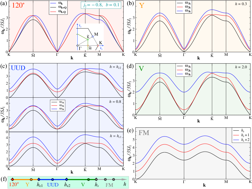
In Fig. 6 we provide plots of magnon eigenenergies for several representative field values from all of the phases sketched in Fig. 4(a) and for the parameters in model (1) and . Energies are in units of and dimensionless field is . All plots are along a representative cut KMK through the full Brillouin zone shown in Fig. 5.
In zero field, , magnetic order is the canonical 120 phase with the symmetry that is spontaneously broken. Since it is broken fully by the choice of the ordering plane and by the spin arrangement within the plane, there are three Goldstone modes that one can observe in Fig. 6(a). As we discuss in some more detail in Appendix B for the 120 case, the three magnon branches that are defined within the magnetic BZ can be related to a single branch defined within the full BZ using “rotated” reference frame for the spin quantization axes. This allows to represent the full spectrum as the “original” branch, labeled by in Fig. 6(a), and two modes that are “shifted” by the ordering vector .
For a finite in-plane field, the symmetry of the model (1) is lowered to by the field. Spontaneous breaking of the symmetry within the Y phase in Fig. 4(a) at results in a single magnon branch with a Goldstone mode and two gapped branches, as is shown in Fig. 6(b) for . A characteristic feature of the gapless branch is an upward curvature of the dispersion in the long-wavelength limit, with .
The UUD phase in Fig. 4(a) is sandwiched between two critical fields, and . Since the symmetry is preserved throughout this phase, the spectrum is, generally, gapped except at the transition points, see Fig. 6(c) that shows magnon spectra at both and and at intermediate . The partially polarized, -preserving UUD state is, in a way, similar to the fully polarized FM phase, with the spectra for the latter for the fields at and above the saturation field shown in Fig. 6(e). Because of the continuous symmetry of the model (1), magnetic field couples to a conserved total magnetization in both UUD and FM cases, which leads to the linear dependence of magnon energies in Fig. 6(c) and (e) on the field. This also makes the transitions at and analogous to the Bose-Einstein condensation (BEC) [51, 52]. We note that the absolute minima of and the corresponding BEC condensation points in the FM case are at the ordering vectors of the three-sublattice order, K, not at the point. To emphasize this feature of the FM phase, the magnon energies in Fig. 6(e) are shown without folding on the magnetic BZ, see also Appendix B.1.
The last phase of the model (1) with a spontaneously broken symmetry that is realized at is the V phase, see Fig. 4(a). Its spectrum is similar to that of the Y phase, having one concave Goldstone and two gapped modes, see Fig. 6(d). It can be seen as interpolating between the spectra of the UUD phase at and that of the FM phase at the saturation field.
IV Kondo coupling and resistivity
In this Section we derive the electron-magnon interaction Hamiltonian, originating from the Kondo coupling, for a general case of a coplanar spin arrangement and present the expression for the electronic transport relaxation rate due to such a scattering mechanism.
IV.1 Kondo coupling
The most reasonable minimal model for the interaction of conduction electrons with the local spins in the magnetic layers of EuC6 is the Kondo coupling
| (45) |
where electron spin operators are with being Pauli matrices. With the external field providing spin quantization axis, it is natural to split (45) into spin-flip and non-spin-flip parts, ,
| (46) | ||||
where are operators of the conduction electrons and indices in the operators of local spins refer to the “laboratory” reference frame associated with the field direction, see Fig. 3 and Fig. 4.
The Kondo coupling is a standard low-energy approximation, which describes interactions of localized spins with electrons at the Fermi surface. In our case, the corresponding electronic states respect the and sublattice symmetries of the graphene layer. In Fig. 2(a), we have demonstrated the folding of the two graphene-like bands, originally affiliated with the vicinities of the and points, onto the proximity of the point in the Brillouin zone of the Eu lattice, see discussion in Sec. II.1. It is only these two bands that cross the Fermi surface and are encoded in our Fermi-operators in (45). Therefore, by construction, our Kondo term accounts for the coupling to a linear combination of orbitals of the surrounding carbons that respects lattice symmetries mentioned above, but are also projected onto the electronic states that belong to these low-energy conduction bands. The couplings to the neighboring carbons also involves other electronic states, but they are unrelated to the states near the Fermi surfaces. Thus, the Kondo coupling in (45) provides the most reasonable minimal description of the interaction of local spins and conduction electrons. In addition, since we treat the two low-energy bands as independent, the coupling to local spins is treated as diagonal in the band index in (45).
For a general coplanar spin configuration in Fig. 4, the local axes are rotated from the laboratory ones (12) to introduce quantized spin excitations for a given spin arrangement. Consider the non-spin-flip part. Here, according to (12), , with being the angle of spin’s -axis on a site with . Upon quantization, converts into two-magnon term, while yields one-magnon emission/absorption. Similarly to the problem of electron-phonon scattering, it is the lowest-order coupling that needs to be considered, unless it is forbidden for a symmetry reason or its scattering kinematics is suppressed. In our case, there are no such constraints and the part is also of the higher order in sense. Therefore, we approximate the local spin operators in (46) by their single-magnon components
| (47) |
where the angle depends on the sublattice.
Using Fourier transform (21) in (46) together with (47), one arrives at
| (48) | ||||
where , is the total number of sites and summation in and is over the full Brillouin zone of the triangular lattice, Fig. 5. We note that the single-magnon non-spin-flip terms are nonzero in the 120, Y, and V phases, in which the angles , because in these states the symmetry of the Hamiltonian (1) is broken completely and a spin-flip does not correspond to a particular spin value.
The last transformation is to the quasiparticle operators given by Eq. (36), which yields
| (49) | ||||
with the matrix elements
| (50) |
One can see that while the structure of the non-spin-flip term in (49) is similar to that of the electron-phonon scattering, the spin-flip part is different as the amplitudes of magnon emission and absorption by the same electron are, generally, different. This is, of course, most obvious in the polarized FM state, in which magnons do have a definite spin, and, therefore, can be emitted only by electrons with the spin and absorbed only by electrons with the spin .
With the electron-magnon couplings explicated in Eqs. (49) and (50), one has a clear path toward a calculation of the electron’s relaxation rate and, therefore, resistivity as a function of the field and temperature.
The derivation of the electron-magnon interaction above and the calculation of the relaxation rate that follows can be repeated for individual particular cases of the 120, FM, and UUD phases with an alternative spin-wave formulation considered in Appendix B. Each of these considerations follows the same structure with a varying degree of simplification compared to the general case described above. While we do not expose these alternative solutions here as they lead to identical outcomes, they do offer an important verification and an analytical insight into the makeup of our solution.
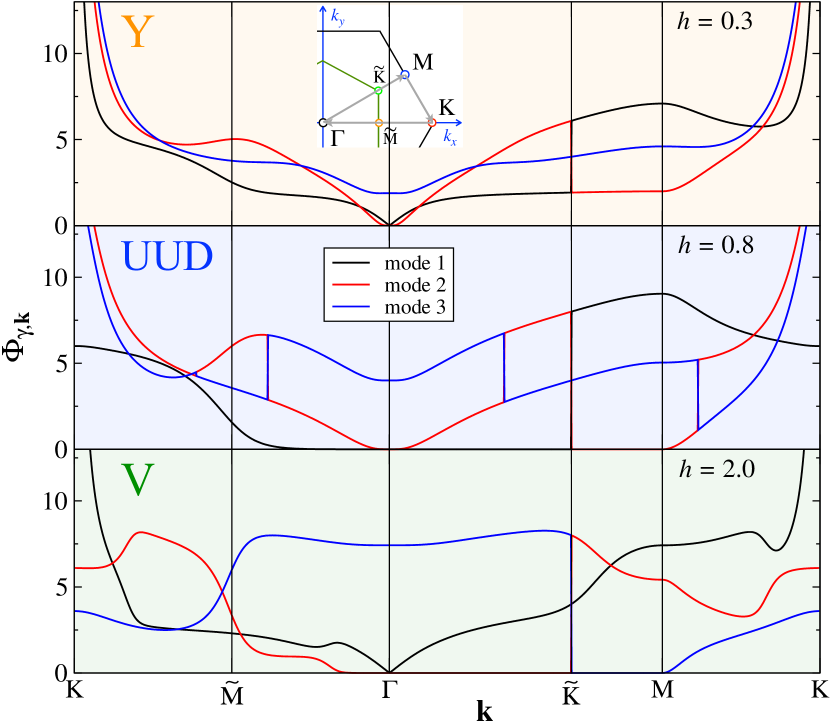
We have repeatedly emphasized the importance of the field-induced changes in magnon energies and in electron-magnon matrix elements for our key results that follow next. With the representative magnon energies shown in Fig. 6, we complement them with the similar representative plots of the combinations of matrix elements given in (53), which enter the integral expression for the resistivity, see Eq. (52) below. In Fig. 7 we show combinations from (53) for the three representative field values from different phases, Y phase at , UUD phase at , and V phase at . The plot is along a representative cut KMK through the full BZ as in Fig. 6 and for the same parameter choices in model (1) as above, and .
Since the numeration of magnon modes in Fig. 6(b)-(d) is from the lowest to highest in energy, the solutions for the matrix elements in Fig. 7 switch between branches whenever branches cross. Some of the crossings are at the high symmetry points and some are not. A general trend that can be observed in Fig. 7 is that some of the matrix elements are strongly suppressed around the point and are either maximal or singular at the point.
An interesting feature of the matrix elements in the UUD phase can be noted. There is no dependence of on the field, only switching between branches according to their numeration. That is, while there is a definite reshuffling of the magnon modes vs field that can be seen in Fig. 6(c), the same combination of matrix elements as depicted in the middle panel of Fig. 7 corresponds to any other point on the magnetization plateau (UUD) phase. This observation provides an interesting connection between the structure of the quasiparticle states, encoded in their wave-functions, and conserved magnetization.
IV.2 Resistivity
Similarly to the theory of electron-phonon scattering in the resistivity of metals, Fermi energy is by far the most dominant energy scale of the problem, perhaps even more so in our case, as the magnon bandwidth, field strengths, and temperature range of interest are all K while –3 eV [31]. Because of that, magnon-induced scattering of electrons is happening within a thin energy shell around the Fermi surface. For the effectively 2D magnetic excitations, transport scattering rate can be shown to reduce to a 1D integral that is limited by that shell.
With the technical details of the Boltzmann equation approach to the electron-magnon scatterings in Eq. (49) delegated to Appendix C and a mild assumption of the circular 2D Fermi surface, we obtain the transport relaxation rate for electrons with both spin projections
| (51) |
where , with being effective electron mass, is a Fermi momentum, and the 1D integral given by
| (52) | ||||
with the 2D momentum parametrization along the 1D contour , Bose distribution function for a magnon with the energy , numerating magnon branches, and abbreviating matrix element contribution
| (53) |
This result in (51)-(53) combines the effort of the entire work in a concise form. It accumulates the solution of the transport theory that proves the validity of the -approximation in our case, implicitly contains the field-dependence of the magnon spectra and matrix elements (50) via the spin angles and parameters of the generalized Bogolyubov transformation (36), incorporates field-induced transitions between different phases, and includes the effect of thermal population of magnetic scatterers on the resistivity. As is discussed in the Section V, contributions of the thermal distribution of magnons and matrix element component (53) are both essential for the resistivity results. While the general expressions (51) and (52) may not be too intuitive, the following consideration will provide essential ingredients for such an intuition.
IV.2.1 Large- insights
The key elements of the physics packed in Eq. (51) can be extracted from the kernel of the integral in (52). We begin by noting that the factor in (52) originates from a suppression of the small-angle scattering processes of electrons in the transport relaxation rate. Thus, the integral is dominated by the large- scattering events that correspond to and . The factor is due to angular integration in 2D and also contributes to an enhancement of the large- contributions.
Further intuition, which also lays out expectations for the results presented in the next Section, is provided by the remainder of the kernel in the second line of (52) taken at a “typical” momentum and in the high-temperature limit, approximating Bose-factors as and omitting an overall prefactor ,
| (54) |
Referred to as “the kernel” below, is a sum over the branch index of the ratios of the matrix elements (53) and magnon energies, taken at . We also note that the high-temperature approximation is closely relevant to EuC6 phenomenology discussed in Sec. V.
The kernel allows one to analyze contributions of different magnon modes to the resistivity and also to compare the relative importance of the spin-flip and non-spin-flip channels in the scattering. While the latter is absent in the collinear UUD and FM phases, it is present in the noncollinear Y and V phases, where , see (50). This partitioning of (54) into the channels is done by separating the non-spin-flip matrix element contribution in from the rest, see (53).
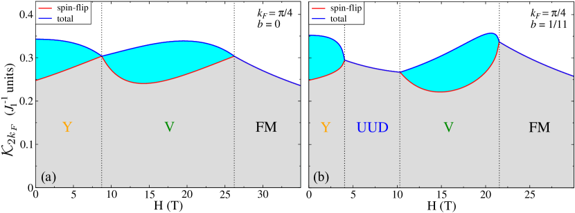
Figure 8 shows (54) vs magnetic field for a representative and for two values of the biquadratic parameter in model (1): (a) Heisenberg, , and (b) . The rest of the parameters are from Table 1, see Sec. II.2.3. In the Heisenberg limit, the UUD phase reduces to a critical point separating Y and V phases. Contributions of the spin-flip and non-spin-flip scattering channels are shaded by different colors.
The key lesson of Figure 8 is that the non-spin-flip scattering channel, although secondary to the spin-flip one, is responsible for an enhancement of in the noncollinear Y and V phases relative to the collinear UUD and FM phases where it is not available. Accordingly, one should expect the higher transport relaxation rates (51) and higher resistivity in these noncollinear phases. Fig. 8 also shows that the biquadratic interaction enhances non-spin-flip scattering and causes stronger variations of the kernel near Y-UUD and V-FM transitions. One can anticipate all these trends to persist in the results for the resistivity discussed in Sec. V.
IV.2.2 estimate and other scatterings
Using considerations of the electronic structure of EuC6 provided in Sec. II.1 and assuming two doubly-degenerate bands with cylindrical Fermi surfaces to describe it, the 3D electronic concentration is related to the value of the Fermi momentum via
| (55) |
where is the interplane distance between Eu layers. With that and some rearranging, the expression for the resistivity can be cast in the following form
| (56) |
in which the von Klitzing constant k and interplane distance set the proper units and the relaxation rate of (51) is made dimensionless by a normalization to the Fermi energy.
One can use the expression for in Eq. (56) with from (51) to estimate the Kondo coupling constant in (45) that is needed to reproduce experimental values of in EuC6. By taking cm from Fig. 1(b) and Å[21], one obtains , which, if matched to the theory results for in Fig. 1(c), yields . By scaling of the value of the Fermi energy in Fig. 2(a) to what it would be for , one has eV and eV. This estimate is of the same order, albeit somewhat larger, than the value 0.15 eV quoted in the early literature [24]. However, it seems that most of the discrepancy could be in the factor of two difference in the definition of electronic spin in the Kondo coupling (45), making the remaining difference rather academic.
Empirically, the resistivity of EuC6 changes from about 2 cm at 4 K, to nearly 50 cm at room temperature, see Fig. 1(b) and Ref. [18]. While the low-temperature value is in the same range as in the other graphite-intercalated compounds, see Ref. [16], the room-temperature resistivity in EuC6 exceeds that of the nearly isostructural non-magnetic GICs such as LiC6 by more than an order of magnitude, clearly suggesting that it is the scattering on magnetic degrees of freedom, such as the ones considered in this work, that must be dominating the usual phonon and impurity scattering [18].
For the phonon scattering effect in the resistivity of EuC6 for the temperature range relevant to our work, the phonon Debye temperatures in various GICs, estimated from the specific heat measurements, range from 300 K to 700 K [16], with the phonon spectrum of graphite [53] suggesting similar value. This implies that the phonon-induced resistivity for K should follow the strongly non-linear Bloch-Grüneisen behavior, inconsistent with experiments. Moreover, as is discussed in Sec. V below, the magnon Debye temperature is about an order of magnitude smaller than that of phonons, making phonon contribution to scattering completely negligible in the relevant low-temperature regime even for an unphysically large electron-phonon coupling. Thus, this consideration suggest a strongly subleading role of phonons in the resistivity of EuC6 at all temperatures.
As is implied by a comparison of our theory results to experiments in Fig. 1 and by the results in the Section V below, one can assume that the “residual” resistivity of about 2 cm at 4 K in Fig. 1(b) is mostly associated with impurity scattering. It is easy to infer from Eq. (56) that this value corresponds to the mean-free path of
| (57) |
which yields cm for and Å[21]. This is about a factor smaller than the mean-free path in pristine graphite, but is of the same order as in the other GICs [16], as the similarity of their residual resistivities has already indicated.
Although many types of defects may play an important role in GICs [54], one can model their effect as that of the screened Coulomb centers of charge- in order to infer an overall nominal impurity concentration. This is in accord with the textbook approach [55] to the impurity-scattering in resistivity. For that, we obtain a modified relation between the mean-free path and impurity concentration for the quasi-2D cylindrical Fermi-surface
| (58) |
with the angular averaging of scattering contained in
| (59) |
where , is a screening length, and is the electronic concentration from Eq. (55). For the doubly-degenerate cylindrical Fermi-surfaces of electrons that we use here as an approximation, one can find the screening parameter as , where is the interplane distance. Using (57) and (58) for corresponding to and lattice constants quoted above, we find that cm corresponds to .
Using the same one can convert impurity concentration per electron to concentration per carbon to obtain , which is about 120 ppm. In graphite, solubility limits of most impurities are very low [56, 57], with the major residual impurities that reach the obtained value often being that of Fe. This observation may provide additional ground for the scenario outlined below in Sec. V.4 in our discussion of the remaining problems, in which we suggest that sizable variations in the residual resistivity versus field may be related to the magnetic nature of the impurities and to the scattering due to spin-textures induced by them.
V Results
With all the elements of our approach and qualitative and quantitative considerations and estimates provided above, we can now offer a detailed overview of the results that follow from our theory. A comparison of the experimental data for the magnetoresistivity in EuC6 vs field with our calculations for the model parameters from Table 1 and for a representative value of is given in Figs. 1(b) and (c). Given the simplicity of our model and potential additional unaccounted effects discussed in more detail in Sec. V.4, the similarity between experiment and theory is rather astounding.
This similarity includes high resistivity in the Y phase and its quick roll-down near the Y-UUD transition, a gentle downward slope of vs in the UUD phase, followed by a smooth rise in the V phase. The temperature evolution of the curves is also consistent with the data, perhaps with an exception of the lowest temperatures. A discrepancy can also be seen in the larger values of in the FM phase and a strong rise toward it near the V-FM transition in the theory results. This is likely due to a proximity to the – phase transition boundary, where interactions between magnetic excitations, neglected in our consideration, become important.
This successful comparison strongly suggests the correctness of the advocated mechanism of the magnetoresistance in magnetically intercalated graphite as dominated by electron scattering on magnetic excitations, which, in turn, allows insights into the nature of such excitations.
In the following, we present further evidence of the success of our theory together with a detailed analysis of the dependence of our results on the key model parameters, such as biquadratic interaction of spins and electron Fermi momentum , summarized in Figures 9–11. This analysis provides implications for the microscopic parameters that should describe EuC6 and also offers a glimpse of the prospective new phenomena that can be induced in intercalated magnetic materials and similar systems by means of the chemical-, pressure-, or gate-doping.
V.1 -dependence of resistivity
We complement our results for the field-dependence of in Fig. 1(c) by the temperature-dependence of at fixed . Our Figure 9(a) shows the results for two field values: , 120 spin state, and for the middle of the UUD phase, . The results are for the same optimal choice of parameters to describe EuC6 from Table 1 as in Fig. 1(c), and for .
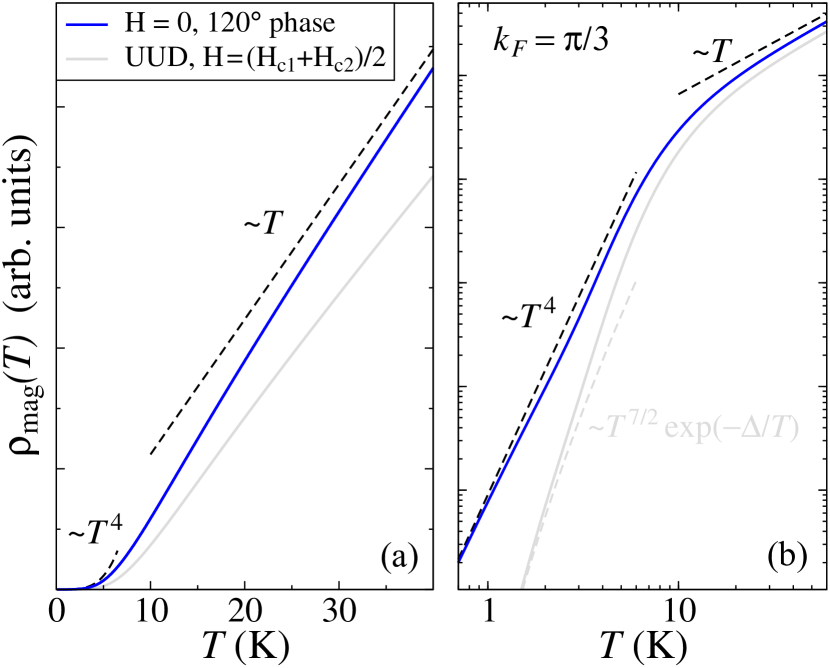
Our Fig. 9(b) shows the same data on the log-log scale in order to emphasize two distinct temperature regimes, the “low-” and the “high-.” The overall energy scale for scattering is set by the magnon bandwidth, which plays the role analogous to that of the Debye energy in the electron-phonon resistivity [55]. Drawing from this analogy, a transition between the low- and high- regimes can be expected at a fraction of the magnetic Debye energy [55, 58, 59], which can be estimated from the magnon spectra in Fig. 6 as with some variation between phases. Using K, see Table 1, and yields K. Indeed, the transition between the two regimes can be observed in Fig. 9 at K.
This consideration implies that the majority of experimental results on EuC6 in Refs. [21, 22, 23], in our Fig. 1(b), which is reproduced from Ref. [18], and in all our theoretical plots are in that “high-” regime, K. The nature of this regime, where resistivity crosses over to a linear- dependence as is indicated by the asymptotes in Fig. 9, is simply an equivalent of the Ohm’s law. Approximating Bose-factors in (52) by their high-temperature limit, , naturally yields . Parenthetically, this also motivates our high- approximation used in the consideration of the kernel in Sec. IV.2.1.
Thus, the nearly-linear -dependence of in EuC6 observed in Ref. [24] above 8 K is simply within the onset of the Ohm’s regime, with no need for an artificial backflow scenario proposed in that work. Needless to say, details of the spectra do not matter at high temperatures and the same dependence should hold for all field-induced phases, as is shown by a comparison of the UUD and 120 states in Fig. 9. Naturally, in very high fields, the field-induced gaps will lead to a freeze-out of the magnon scattering.
The low- regime is a bit more subtle and depends on the magnetic phase. The case of the state and, by proxy, of the Y and V phases with the Goldstone modes that are linear at low energies, , see Fig. 6(a), (b) and (d), is very much similar to the textbook case of acoustic phonons. For the state, one can show from Appendix B.2 that the matrix element contribution (53) associated with the coupling to such a mode is also linear in in that limit, . Then, a simple power-counting in (52) for using , yields a 2D analogue of the Bloch-Grüneisen asymptotic regime shown in Fig. 9.
As opposed to the gapless phases, the UUD and FM phases are gapped away from the transition points, see Fig. 6(c) and (e). Thus, one can expect to see an activated behavior of the resistivity, , at sufficiently low temperatures. While this regime can be visible in Fig. 9(b), in practice its detection requires reaching temperatures . There is also an additional smallness due to a prefactor of the exponent associated with a suppressed coupling to the lowest mode, . An estimate for the gap in the middle of the UUD phase for EuC6 gives K, providing a guidance for the future observations.
The locus of magnon momenta that are involved in the scattering depends on the value of as we discuss below. However, in the field-polarized FM case, it is, generally, away from the energy minimum in Fig. 6(e), leading to a larger gap in the exponent, which is further increased by the Zeeman energy away from the saturation field, accompanied by a more favorable prefactor , so the freezing-out should be readily observable in the FM phase at higher temperatures.
Lastly, one can naively expect a power-law that is different from near the Y-UUD and UUD-V transition points as both are affiliated with the BEC-like transitions, in which magnon energy is quadratic, , see Fig. 6(c). Although we refrain from discussing it in any significant detail, the situation is more complicated as the coupling to these BEC modes is different at and . In the first case the coupling vanishes, maintaining an exponential trend due to higher energy modes, while in the second case it indeed leads to a different power-law due to a suppressed coupling, .
Altogether, the consideration given above presents further evidence of the validity of our theoretical approach, providing a physically transparent description of the temperature-dependence of the resistivity of EuC6 in the previously accessed temperature regime. It also invites further such studies in finite fields and especially at lower temperatures, where resistivity should be a sensitive probe of the spin excitation spectra.
V.2 Magnetoresistivity vs biquadratic-exchange
The discussion provided below serves two goals. First is to investigate how prevalent are the strong anomalies in the magnetoresistivity, vs , in the model of the conduction electrons coupled via a coupling (45) to the spins that are described by the Heisenberg-biquadratic model (1). Second is to demonstrate that the magnetoresistivity of EuC6 is consistent with the substantial biquadratic-exchange parameter in such a model.
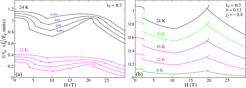
In Figure 10, we present the transport relaxation rate vs field obtained from (51) for several representative temperatures, Fermi momentum , and exchange parameters from Table 1, except that now we vary the key biquadratic-exchange parameter . The corresponding magnetoresistivity is related to these results by a dimensional constant factor, see Eq. (56).
Figure 10(a) shows two sequences of curves, offset for clarity, with the biqudratic exchange increasing in nearly equal steps from the Heisenberg limit, , to the value that we use as an optimal choice for EuC6, see Sec. II.2.3. Figure 10(b) shows results for the biquadratic exchange that substantially exceeds the “critical” value , which corresponds to a change of the Y-UUD and V-FM transitions to the first-order type as discussed in detail in Sec. II.2.2 and Appendix A.
The evolution of with in Fig. 10(a) features already anticipated trends. First, the opening of the -magnetization plateau (UUD) phase away from the Heisenberg limit, see Sec. II.2, is clearly visible. Second, the results in Fig. 10(a) are in a close accord with the behavior of the kernel, discussed in Sec. IV.2.1 and illustrated in Fig. 8, providing an explicit confirmation that the transport relaxation rate and magnetoresistivity are dominated by the scattering processes.
The key observation from the results in Fig. 10(a) is that strong roller-coaster like variations in magnetoresistivity, such as the ones observed in EuC6, must be associated with the nearly critical values of the biquadratic exchange within our model. Although some aspects resembling strong variations and indicating clear differences of vs dependence between different phases can already be observed in the pure Heisenberg model, see, for example, a kink-like feature at the Y-V boundary in the upper curves in Fig. 10(a), others are much less pronounced, see a rather small change of slope at the the V-FM transition at in the same results.
Our Fig. 10(a) demonstrates that the role of the biquadratic term in model (1) goes far beyond just establishing the UUD phase boundaries, which are clearly marked by the kinks in . With increasing , the Y-UUD transition becomes steeper upon shifting to the lower fields, showing a divergent derivative for that is related to a similar behavior of spin angles in Fig. 12. Still, the biggest change takes place at the V-FM transition, which too becomes weakly first-order, as is elaborated on in Appendix A. Here, the field-dependence evolves from a nearly featureless one in the Heisenberg limit to a “shock-wave”-like shape for . In contrast, the UUD-V transition remains continuous throughout these transformations, although the slope of at also changes visibly.
Increasing beyond the critical should lead to a hysteresis in the magnetoresistance. Figure 10(b) illustrates the case of . These results are obtained by using the local stability of the solutions for the magnetic configurations, of their corresponding spin-wave energies, and of electron-magnon matrix elements within the overlap regions of the coexisting phases. For example, from within the Y phase, the Y magnetic configuration persist up to , as is described in Appendix A.1. From within the UUD phase, the same field region can be accessed starting from . Therefore, in the overlap region, , the relaxation rate can be calculated in two different ways, resulting in the sizable discontinuities in Fig. 10(b), indicated by vertical dotted lines marking the overlap intervals of for the Y-UUD and for the V-FM transition.
We note that the transition regions and discontinuities in Fig. 10(b) are only illustrative. As is discussed in Sec. A.1, the transition between the two overlapping phases should take place at , at which the energies of the two phases become equal. At a finite temperature, a proper consideration of the first-order transition should include entropic contribution to the free energy of the competing phases. In addition, one can expect the co-existence region to be affected by secondary anisotropies that are neglected in our minimal model. Nonetheless, we believe that Fig. 10(b) faithfully represents a qualitative effect of a strong biquadratic interaction on the magnetoresistance across the first-order transition.
Altogether, the results presented in this section provide an important overview of the characteristic evolution of the magnetotransport within the model of electrons coupled to the spin subsystem, which is described by the Heisenberg-biquadratic model.
As is discussed in Sec. II.2.3, the microscopic parameters of the spin model (1) describing EuC6 are determined entirely from the thermodynamic quantities, such as critical fields and transition temperature. Therefore, for claiming a success of a theoretical description it is crucial that the resulting set of microscopic parameters yields distinctive features that are in accord with a wider phenomenology of the material, especially the one that involves less trivial quantities such as dynamical response and transport. We can claim such a success here, as the parameters chosen to describe EuC6 in Table 1 are also the ones that produce sharp, nearly singular features in magnetoresistivity results that follow from our theory and also match closely the observed ones.
V.3 Magnetoresistivity, role of
Two more aspects of our study merit further discussion. First, as is mentioned in Sec. II, the electronic band filling fraction in EuC6 and the Fermi momentum parametrizing it are not well-determined. While the nominal Eu2+ valence naively implies a large Fermi surface, the electronic structure and angle-resolved photoemission study [31] suggested a substantially smaller electron fraction in the relevant carbon orbitals and a smaller . We would like to weigh in on this subject, with the magnetoresistivity in our model arguing for a still somewhat smaller Fermi surface, with .
Second, much of the interest in the synthetic materials in general and in the graphite-derived systems in particular is due to a significant flexibility regarding electronic density manipulation. Then, in addition to varying parameters of the spin model, it is also important to explore the outcomes of our theory in a wider range of electronic parameters in order to anticipate potential new effects that can be accessible due to such a flexibility. To that end, we discuss some of the larger- results.
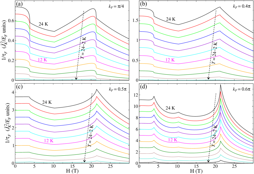
Our Figure 11 shows the constant- curves of the transport relaxation rate vs calculated using (51) as in Fig. 1(c) and Fig. 10 for a set of representative temperatures from K down to K in 2 K steps. Results are for the model parameters from Table 1 which describe EuC6, and for the four different values of the Fermi momentum, , , , and . In this case, the field-independent constant factor that relates to magnetoresistivity , Eq. (56), is different for the four sets as they correspond to different electronic concentrations via (55).
Consider results in Fig. 11(a) first. All of the features in the data are the same as in Fig. 1(c) and as discussed in Sec. V.2 for Fig. 10(a), including the steep Y-UUD transition, a “shock-wave” feature at the V-FM boundary, and a decline in the FM phase due to the Zeeman-induced gap that is depleting magnon population. In agreement with the analysis of vs in Sec. V.1, the temperature-induced offset of the curves is nearly linear in except for the lowest sets.
On a closer and more quantitative side, one can argue that in terms of the overall trends in magnetoresistivity curves, the results in Fig. 1(c) provide a somewhat better fit to the EuC6 data in Fig. 1(b) than the ones. Moreover, to match experimental data, the decrease of requires a nearly proportional increase of the Kondo coupling constant (45) relative to the Fermi energy, , thus restricting from being too small.
A surprising trend starts being revealed by the results for the larger in Fig. 11(b). Although the features in the constant- curves are qualitatively similar to the case, changes at the transitions are less steep and less like the ones in the experimental data in Fig. 1(b). They are nearly gone for the Y-UUD boundary in the results in Fig. 11(c) and the V-FM transition for this is also marked by the spike-like structures, certainly unlike anything observed in EuC6. The results in Fig. 11(d) complete this unexpected trend, with all the transitions, including the formerly rather featureless UUD-V one, showing spikes.
These qualitative transformations signify a change in the dominant scattering that contributes to the resistivity. Regardless of its nature, which we discuss below, an immediate outcome of this analysis is in the phenomenological restriction on the size of the Fermi surface in EuC6. As was described in Sec. II.1, the trigonally warped Fermi surfaces from the band structure in Ref. [31] have the extent from to , in a qualitative agreement with a rigid-band estimate assuming circular Fermi surface and per Eu2+ doping of the carbon bands that gives , see also Fig. 2. However, the magnetoresistivity of EuC6 within our theory suggests a still smaller Fermi surface with an optimal near . These results invite more research into the band structure and direct measurements of the Fermi surface of EuC6.
To understand the transformation of the relaxation rates with in Fig. 11, we need to return to the analysis of in Eq. (51) and in Sec. IV.2.1. Because of the hierarchy , electrons participating in a conduction process scatter between momenta that are in a close vicinity of the Fermi surface. With an assumption of the circular 2D Fermi surface, the magnon momenta that are involved in such a scattering also form a circular locus of points in the space, see Fig. 13(b) and Fig. 16 in Appendix C. These momenta extend from to the maximum of , with the small-momentum contribution to the transport scattering rate in (51) suppressed and large-momentum contribution enhanced, as is discussed in Sec. IV.2.1.
Then it follows for the case that the typical large-momentum “”-magnons, responsible for most of the scattering, are from the set of near . Referring to the Brillouin zones in Fig. 5, this value corresponds to the proximity of the point of the magnetic Brillouin zone and to the high-energy magnons near the maxima of , see Fig. 6.
However, further increase of drives the extent of the -contour outside of the first magnetic BZ and also brings the -magnon energy down. Then, the truly “dangerous” value of the Fermi momentum of the circular Fermi surface is , as it allows magnon momenta to reach the corners of the full Brillouin zone, and , which correspond to the ordering vector of all ordered phases, , with gapless or nearly gapless modes. Thus, it is the approach of , or, rather, , which is responsible for the dramatic changes in Fig. 11 from (a) to (d).
This analysis also shows that at a given , the population of the relevant scatterers for is lower than that for the larger values, which explains an order-of-magnitude enhancement of from in Fig. 1(c) to in Fig. 11(d) that is only partially accounted for by the factors in (51).
Since the arguments above relies only on , they suggests a degree of universality. Specifically, we argue that in all gapless phases should diverge in this limit as , with a field-dependent prefactor, leading to an overall increase of the relaxation rates observed in Fig. 11(d). In addition, the behavior of should apply equally to the pure Heisenberg case, which offers an opportunity for a quantitative analytical insight. Using expressions for the FM and 120 phases from Appendix B and high- limit for the Bose factors in (52), neglecting and , and expanding near , after some algebra, indeed yields for the FM phase at the gapless point. The result is the same for the 120 phase at , but smaller by a factor 3/4.
Since is the transition point that exhibits spike-like features in Fig. 11, while the 120 state is away from the transition, this result confirms our hypothesis that the entire set of is divergent, or nearly divergent in the weakly gapped UUD phase, with the spikes being a quantitative effect that is associated with Goldstone modes at the transitions compared to modes inside the gapless Y and V phases. We can also verify that the factor 3/4 between the and (120 phase) points is indeed in a reasonable accord with the results in Fig. 11(d). The divergence is also consistent with the difference between and results at in Figs. 11(c) and (d).
This study of the divergence brings in one more important aspect of the problem that has been neglected so far. We use a fairly reasonable and certainly simplifying assumption of the cylindrical Fermi surface. However, by itself this assumption does not automatically make independent of the direction of the electron momentum , with the angular-dependence originating from the discrete lattice symmetry that is still encoded in the spin excitations and electron-magnon matrix elements.
As may be clear intuitively, the reason for this issue to be important in the context of the divergence is that the “dangerous” -vectors correspond to the discrete points (BZ corners) in the momentum space, see Fig. 5, leading to the truly divergent only for these directions. This subject is considered in Appendix C.4.2 for a closely related quasiparticle relaxation rate , for which the effect of angular dependence can be taken into account without any additional approximations.
In Appendix C.4.2, we demonstrate that the effect of the angle-dependence in is really negligible up to and even for it is still very modest, confirming the accuracy of our results presented in this work and justifying our initial approximation that omitted this effect.
Given the limitations of the cylindrical Fermi-surface approximation, which should become problematic for larger , and possible effects of the Fermi-surface reconstruction at the magnetic zone boundaries, it is not entirely clear whether the true divergences will survive, but they may still have strong effects even if avoided. This points to an interesting venue of potential studies of the magnetic scattering effects in the large-Fermi-surface EuC6, induced by the chemical-, pressure-, or gate-doping.
Some of the considered phenomenology is reminiscent of the “hot spots” phenomena, much discussed in the theory of cuprates [60], where certain parts of the Fermi surface are suggested to experience strong scattering due to the low-energy magnetic excitations with a particular -vector. It is not unthinkable that the suggested further studies of the large-Fermi-surface EuC6 may also be able to shed a new light on this important problem.
V.4 Outlook
We would like to reiterate that the present study has provided a thorough consideration of one of the iconic models in frustrated magnetism, the triangular-lattice Heisenberg model, enriched by the biquadratic exchange and coupled to conduction electrons, with the goal of understanding magnetoresistivity throughout its phase diagram in an external magnetic field. The use of this model as a microscopic description of EuC6, with additional approximations for electron bands and parameters estimated from experimental critical fields and temperature, is clearly a simplification. Yet, the evidence of the success of such a description is undeniable, with many, if not most, features of the magnetoresistivity reproduced, also leading to constraints on the model parameters for both localized spins and electron densities discussed above.
However, the presented description is not complete. Below, we briefly discuss other possible terms in the model that might be missing, their expected effects, possible sources of the remaining discrepancies of our theory with the experimental data, and desirable future studies.
First additional term in the spin model (1) is the ring-exchange term (2), inspired by the early works [61, 62], see a discussion of it and its secondary role for EuC6 in Sec. II.2. According to our estimates in Table 1, the ring-exchange is about three times smaller than the biquadratic term. Since the symmetry of the model is unaltered by it and the field-induced spin-angle dependencies on the parameters that make transitions first-order are very similar to the biquadratic-only case [21], it was reasonable to neglect it. The only unexplored outcome of the ring-exchange term is a possible stabilization of an additional magnetic state between V and FM phases, with some evidence of such a phase in EuC6 suggested by the data, see Fig. 1(b) and Ref. [18].
Next is the anisotropy in the and terms, which is necessary to explain very different magnetization behavior for the in- and out-of-plane field direction [18]. Given close values of the saturation fields for these directions and nearly isotropic g-factor, it is expected to be relatively weak, at the level of 10% [21], see also Sec. II.2. However, unlike the ring-exchange, it lowers the symmetry of the model. Therefore, for the in-plane field, none of the considered phases will have the true Goldstone modes, and gapless excitations will exist only at the field-induced transitions. This is going to alter the low- behavior of the resistivity discussed in Sec V.1, and also change the dynamical critical exponent at all critical fields from the BEC-like (, ) to the relativistic-like (, ). However, as most of experimentally-relevant theory results is pertinent to the “high-” regime, see Sec V.1, the effect is expected to be secondary on them. We have performed a limited study of anisotropic model for some of the phases, and found no qualitatively significant differences from the Heisenberg limit results in that regime even for strong anisotropy.
Since Eu2+ spins are large, the dipole-dipole interactions are not necessarily negligible. However, using the analysis of Ref. [63] and the size of the unit cell of EuC6, we estimate this term to be at least an order of magnitude smaller than the values of the exchanges. Since the dipolar terms also break spin rotational symmetries, one can expect effects similar to that of the anisotropy.
The spin and electronic degrees of freedom are not purely 2D in EuC6, with the 3D interplane spin couplings estimated to be of order in Ref. [18]. While nominally essential for the finite Néel temperature, the effect on the spin excitations can be expected to be minimal. However, even if they are small, both electron and spin 3D dispersions can be crucial for the softening of the singularities discussed in Sec. V.3.
Perhaps the most significant difference of the outcome of our theory from the magnetoresistance data in EuC6 in Figs. 1(b) and (c) is the larger values of in the FM phase and a strong rise toward it near the V-FM transition. An obvious reason for the discrepancy is the neglect of the temperature dependence of the phase transition boundaries in our approach. While it can be dismissed for the Y-UUD and UUD-V boundaries, for which the results are in a close accord with the data, transition at the V-FM boundary has a substantial downward suppression with . One of the possible approaches, which we leave for future studies, is to include temperature dependence of by accounting for the interactions between magnetic excitations that are ignored in our consideration.
A less straightforward suggestion is related to the form of the Kondo coupling (45). We have two Fermi surfaces, originated from the downfolding of two Dirac graphene bands onto the Brillouin zone of the Eu-lattice. The coupling to local spins is treated as fully diagonal in the band index in (45). This may, or may not be the full story, with an intriguing prospect that the spin arrangement can permit or forbid interband scattering. This is again an interesting subject for a further investigation.
Another notable difference of our results in Fig. 1(c) from the data in Fig. 1(b) is at the lowest temperatures that are accessed experimentally. While scattering on magnetic excitations dies out in our theory, magnetoresistivity data retains sizable differences between magnetic phases. One of the scenarios is due to a feedback of the spin orders on the electronic density of states, producing a different imprint onto the resistivity in different field-induced phases. Further studies, with a help of electronic structure calculations, can be envisioned here.
A different scenario for the same effect involves a compelling picture associated with the impurity-induced spin-textures [64, 65], which generally arise in frustrated spin systems due to magnetic couplings that are modified in the presence of impurities. While the impact of such textures on the dynamical properties has been recently investigated [66, 67], their effect on the resistivity in the field-induced phases is simply unknown. However, one can expect the spin-textures to exist readily in the noncolinear and be suppressed in the collinear phases [64, 66], suggesting a profile that is similar to the one observed in the magnetoresistivity. Needless to say, this is a yet another direction for future investigations.
The hybridization between electrons of Eu2+ ions and conduction electrons also asks for additional insights from the first-principles perspective, as we comment in Sec. II.1 in explaining our choice of the “minimal” model description of the Fermi surfaces in EuC6. This subject, as well as the role of the valence fluctuations, does require separate studies from both experiment and theory, which are well outside the scope of the present work. The success of the proposed effective spin model with the Kondo coupling in explaining the “roller-coaster” resistivity suggests that both of these open issues, while interesting on their own, may only be relevant to the low-energy effective model at the level of phenomenological parameters.
Our results can be of a direct relevance to the graphite-derived and related materials of a significant current interest that discuss realizations of the conducting electrons that are Kondo-coupled to localized spins in frustrated lattices, such as transition metal dichalcogenides [34, 35, 36]. However, a different physical regime dominated by a large Kondo temperature may intervene and prevent the ordering in a frustrated magnetic system, placing the physics of the case in a new regime. The details of how these energy scale compete, whether the present discussion holds, and what new insights are required in this case needs further investigation.
We conclude this Section by suggesting several extensions of experimental work in EuC6. As is discussed in Sec. V.1 and above, precise low-temperature measurements would provide a significant source of information on the field-induced transitions to and from the UUD phase that would allow to study intriguing critical behaviors and help determine the effective model more precisely. As we have expounded on in Sec. V.3, the tunable- experiments can allow to study singular behavior in resistivity that may have significant implications to other systems, and as is briefly mentioned in Appendix C.4.2, a significant violation of the Wiedemann-Franz law can be expected at the field-induced transitions in EuC6.
VI Summary
The main goal of the present study has been to develop a microscopic theoretical description of the highly dramatic evolution of the resistivity in EuC6 with the magnetic field. The results and discussions presented in the prior sections provide a strong affirmation that we have succeeded in that goal, with our results capturing most of the qualitative and quantitative features of the experimental data. This success is based on a physical picture of the scattering of electrons from the graphene-derived bands of the carbon layers by spin excitations from the triangular-lattice Eu-planes.
In the course of this work, we have provided a thorough theoretical investigation of the ground states, field-induced phase transitions, spin excitations, and their couplings to the conduction electrons in the paradigmatic two-dimensional triangular-lattice antiferromagnet with a biquadratic exchange, throughout its phase diagram. Our effort highlights the virtues of the full-scale microscopic approach to the problem, not only to the spin model, but also to the transport formalism for the spin-flip and non-spin-flip channels, allowing rigorously obtained numerical results to receive comprehensive analytical and physical insights and interpretations.
The research advanced in the present study yields predictions of new field-induced and doping-induced phenomena in magnetically-intercalated graphite and related systems, also offering an inspiration for bringing together different approaches in the search of new effects in the graphite-derived artificial magnetic materials. We anticipate our effort to be relevant to a broader research in metallic magnets and to provide significant technical guidance for the similar theoretical studies. Presently, our study invites more research into EuC6 electronic, thermodynamic, transport, and magnetic properties.
Lastly, our work has advocated resistivity measurements, combined with a detailed theoretical analysis, as a very informative probe of not only field-induced phase transitions, but also of the unconventional spin excitations in magnetic materials. We believe that synthetic 2D materials may become a significant source of potentially novel insights into the nature of exotic spin excitations such as, for example, fractionalized spinons in a quantum spin liquid.
Acknowledgements.
We are indebted to Roser Valentí and Vladislav Borisov for a fruitful discussion regarding electronic structure of intercalated graphite and for sharing their unpublished data that provided an important first-principles and moral support to our Fermi-surface consideration. We would like to wholeheartedly thank KITP for the semi-virtual hospitality during the workshop of the pandemic-impacted Fall of 2020 when the bulk of this work was completed. An unexpected and enlightening encounter by one of the authors (A. L. C.) with Urobatis Halleri during the partial in-person attendance have undoubtedly impacted the reported results. O. A. S. thanks Hassan Allami and Dima Pesin for discussions of experiments on EuC6 and initial attempts at the theoretical formulation of the problem. A. L. C. is grateful to Pavel Maksimov for a substantial Mathematica help and to Ilya Krivorotov for an illuminating discussion regarding possible values of the dipole-dipole terms. The work of A. L. C. was supported by the U.S. Department of Energy, Office of Science, Basic Energy Sciences under Award No. DE-SC0021221. The work of O. A. S. was supported by the National Science Foundation CMMT program under Grant No. DMR-1928919. KITP is supported by the National Science Foundation under Grant No. NSF PHY-1748958.Appendix A First order transitions
Here we describe analysis of the first order Y-UUD and V-FM transitions. We focus on the Heisenberg-biquadratic model (1) and provide some technical details on the classical ground states introduced in Sec. II.2.1.
A.1 Y-UUD transition
Without the ring-exchange term, , equation on in the Y phase, Eq. (4), reduces to
| (60) |
A substitution gives
| (61) |
Comparison with the trigonometric identity
| (62) |
leads to the solution for
| (63) |
It is now easy to check that the Y-UUD transition for is continuous and takes place at , see Eq. (5), at which . For , the Y phase remains locally stable up to a critical field , see Eq. (6), which is found from the condition that the argument of in (63) reaches the maximal value of .
Given that the UUD phase remains locally stable for all , we observe that field interval determines the overlap region of the Y and UUD phases.
Within our approach, however, the actual transition between the two phases takes place when the classical energies of the two phases become equal. This defines another field, , which can be found as follows. First, with the help of (60), the per-site energy of the Y phase can be simplified to a quadratic form of
| (64) |
which, upon equating with the energy of the UUD phase , yields
| (65) |
For a given , the right-hand sides of (65) and (63) determine the transition field . The solution is easily obtained numerically using MATHEMATICA.
For our choice of , see Table 1, which is only slightly larger than , the resultant critical fields are nearly indistinguishable from each other: . For the larger values of , the three fields become sufficiently different and allow one to study resistivity hysteresis. For example, for considered in Sec. V.2 we have .
A.2 V-FM transition
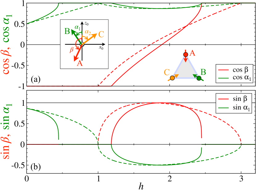
In the V phase, denoting , introducing , and rewriting Eq. (8) as a cubic equation for the variable defined in the interval yields
| (66) |
This equation is solved by mapping to the same identity (62) as above, with the result given by
| (67) |
from which the angles are obtained as
| (68) |
It is easy to check that the V-FM transition is continuous for , with the same as above, and the critical field of the transition is given by , see Eq. (9). For , V phase remains locally stable up to a larger field , which is found from the argument of in (67) being equal to .
Similarly to the case of the discontinuous Y-UUD transition described above, the actual V-FM transition field is found by equating energies of the V and FM phases. Some tedious algebra gives the energy of the V phase
| (69) |
while . Solving numerically, with given by (67), we find that the actual transition field satisfies .
For used in our work, we find , which are, again, essentially identical. For considered in Sec. V.2, these fields become .
Appendix B Particular cases
With the general spin-wave approach for the coplanar three-sublattice states outlined in Sec. III.1, it is still immensely useful to have a fully analytical approach developed for some of the states. This is for the sake of both explicit analytical results and for an independent verification of the partially numerical approach of Sec. III. For the fully polarized FM and 120 states, a single-sublattice formulation of the SWT is possible. For the UUD state, the Hamiltonian matrix in (25) can be reduced to matrix and solved in a compact form.
B.1 Polarized state
In the fully polarized FM state, see Fig. 4(a), all angles are the same, . In the absence of the easy-plane anisotropy, the off-diagonal () terms cancel out and the LSWT Hamiltonians in Eqs. (13)–(20) reduce to a tight-binding form similar to that of (20). Since there is no distinction between the sublattices in this case, a Fourier transform of the Holstein-Primakoff bosons
| (70) |
where is the total number of sites and belongs to the full Brillouin zone of the triangular lattice, is sufficient to diagonalize the LSWT model. The magnon energy is
| (71) |
where , , as before, is given in (35), and
| (72) |
Here, consideration of the Kondo coupling (45) simplifies substantially as the single-magnon spin-conserving terms in the electron-magnon interaction in (46) are not present, laboratory and local spin axes are the same, and all sublattices are equivalent. Using Fourier transform (70) in (46) with (47) and yields
| (73) |
where as before. The spin-flip scattering term is simple, with a matrix element containing no momentum-dependence.
According to Appendix C.3, the spin-flip scattering straightforwardly leads to the relaxation rate in the form of Eq. (51) with the 1D integral in (52) taking the form
| (74) |
with the same momentum parametrization along the 1D contour and Bose distribution function with the magnon energy from Eq. (71).
Given the simplicity of the polarized FM state, it may be instructive to demonstrate a relation of the single-sublattice formalism to the general three-sublattice one described in Secs. III.3 and III.4, as the latter is supposed to give an identical description.
For all spins polarized, , the off-diagonal term in the Hamiltonian matrix (25) and
| (75) | ||||
where is a identity matrix and
| (79) |
with from (35). Since , the three magnon branches have the energies
| (80) |
where are the eigenvalues of . A straightforward algebra with (79) gives and , with from (72) and . Thus, the three magnon branches are the “original” single-sublattice result in (71), , and the other two are “shifted” by the ordering vectors, .
In the single-sublattice treatment shown above, the one-magnon coupling involves () operators from (70) with a constant matrix element, see Eq. (73). In the three-sublattice approach, matrix elements (50) of the general form of electron-magnon coupling in Eq. (49) require the knowledge of the Hamiltonian eigenfunctions. In the polarized FM case, anomalous terms in the transformation to quasiparticles (44) are absent, , and all angles are , immediately simplifying (50) to just
| (81) |
with the matrix elements , where the matrix of vectors should diagonalize in (79). A simple algebra yields
| (82) |
for the “original” and “shifted” , respectively; here .
Because of the local nature of the Kondo interaction, the matrix element of the coupling to an eigenmode in (81) is simply proportional to the sum of the components of a corresponding vector, . Thus, as it trivially follows from (82), the resultant matrix elements of the coupling to the “shifted” modes are identically zero and only the “original” -mode contributes to (81) with .
Needless to say, this renders the coupling Hamiltonians in the single-sublattice and three-sublattice treatment, (73) and (81), equivalent. Their resultant scattering rate is given in (51) and (74).
A closely associated problem is the relation between the single-sublattice operators () to the three-flavor operators (). A simple algebra gives
| (83) | ||||
with the same . These expressions are general and apply to the other cases where both single- and three-sublattice approaches are possible, such as the 120° case discussed next.
B.2 120° state
For the 120° state, see Fig. 4(a) for a sketch, the angles that define spin configuration and transformation to the local reference frame in Eq. (12) can be written as
| (84) |
where, according to the choice in Fig. 4, , with , , and , see Fig. 3, and as before. As a result, all mutual angles are the same up to a sign, , making the LSWT Hamiltonian terms in (18) the same on each bond and rendering the division of the lattice in three sublattices unnecessary. The Fourier transform (70) leads to a standard LSWT Hamiltonian [68, 69, 70, 71, 72]
| (85) |
where
| (86) |
with from (72) and magnon energy with the parameters of the Bogolyubov transformation given by
| (87) |
Similarly to the FM phase considered above, the relation of the single-sublattice branch to the three-sublattice energies is straightforward, with the three branches given by the “original” and the two “shifted” ones, , see Fig. 6(a).
The relationship of the three-flavor operators () to the single-sublattice operators () is the same as in Eq. (83) as it is simply a relation between one- and three-sublattice Fourier transforms in (21) and (70). The eigenvectors of the generalized Bogolyubov transformation in the three-sublattice case (36) are related to the single-sublattice ones in (87) via a combination of shifts by and the phase factors as in (83) in the latter.
The electron-magnon Hamiltonian is obtained from the Kondo coupling (46) using spin-rotation transformation (12) with the angles (84), subsequent spin-operator bosonization, and Fourier (70) and Bogolyubov (87) transforms. Because of the non-collinear structure, it contains both spin-flip and non-spin-flip terms that have the same structure as the general form of electron-magnon coupling in (49), which we will not rewrite here.
B.3 Plateau state
The up-up-down (UUD), or magnetization plateau state is special as it does not break rotational symmetry about the field direction, with the spins parallel (up) or antiparallel (down) to the field. For our choice in Fig. 4, sublattice spins are down, , while and spins are up, . With these angles, six out of twelve independent matrix elements in the matrices and (32) of the Hamiltonian matrix (25) vanish and the remaining six are complementary, suggesting a rearrangement in the vector-operator of the Holstein-Primakoff bosons that allows to reduce the rank of the Hamiltonian matrix to ,
| (90) |
where is the rearranged vector-operator with the Hamiltonian matrix
| (94) |
and matrix elements given by
| (95) | ||||
with all constants as before and and from (35).
This approach, first employed in Ref. [20], has been used in a number of more recent works [40, 41]. Physically, such a rearrangement takes advantage of the conservation of magnetization in the UUD state due to remaining symmetry for the Heisenberg spins, which makes creation (annihilation) of spin flips in the down-sublattice equivalent to the annihilation (creation) of spin flips in the up-sublattices.
The standard diagonalization procedure of (94) now concerns , where is a diagonal matrix . The characteristic equation yields
| (96) |
which is a cubic equation on with real coefficients,
| (97) | ||||
that can be solved in a number of standard ways [43], with the three roots giving magnon eigenenergies in units of . At the point, analytic solution of (96) simplifies considerably, making explicit the linear field-dependence of the magnon energies throughout the UUD phase. Note that the numeration of the magnon branches in Fig. 6(c) is from the lowest to highest in energy, not necessarily according to the numbering of the solutions above.
The transformation from Holstein-Primakoff bosons in (90) to the quasiparticles is similar to the generalized Bogolyubov transformation in (36)
| (98) |
but without the “anomalous” terms and with the “mixed” original and quasiparticle operators and normalization that respects the metric
| (99) |
where .
The transformation (98) from to vectors, written in a matrix form is
| (100) |
where the transformation matrix is given by the normalized eigenvectors of that can be obtained via a somewhat tedious, but straightforward diagonalization procedure using explicit form of in (94), yielding
| (104) |
with
| (105) | ||||
where are the eigenvalues obtained from (96) and (97). While somewhat cumbersome, the outlined formalism allows to perform calculations without relying on numerical matrix diagonalization procedures.
The derivation of electron-magnon coupling and relaxation rate in the UUD phase bears a lot of similarity to the polarized FM case in its three-sublattice formulation, see Sec. B.1. Because of spin collinearity, only spin-flip scattering is present, with either emission or absorption
| (106) |
where as in (98) and matrix elements , with vectors from (104).
As in the polarized FM case, the coupling to a mode in (106) is given by the sum of the components of a corresponding vector, , but without further simplifications that follow in the FM case.
Appendix C Transport formalism, approximation
Transport theory, including its Boltzmann version, is an essential chapter in most of the advanced condensed matter textbooks [55, 58]. Discussion of the electron-phonon scattering, which controls resistivity of metals in a wide range of temperatures, is also a necessary part of the story. Still, the technical aspects of its theory are usually avoided in this context, opting for some physically motivated but not rigorous considerations. While some of the required steps may indeed seem sufficiently cumbersome to justify such an approach, in the following narrative we would like to dispel this accepted aura from the subject and outline a step-by-step derivation of the transport scattering rate under the assumption of the quasi-elastic scattering. In the process of doing so, we also provide a solution of the problem at hand, that is, make available a compact expression for the electron-magnon scattering rate in a 2D setting relevant to EuC6.
C.1 Basics and conventions
For an electric current, the key quantity to find from the Boltzmann formalism is , a deviation of the non-equilibrium distribution function from the equilibrium one, where is a Fermi-distribution function. Then, the current density is
| (108) |
where is the electron velocity.
The linearized Boltzmann equation (LBE)
| (109) |
allows to determine in the linear-response approximation, here is an electric field, is a collision integral, and we ignore electron spin for a moment.
The crucial step is the relaxation-time approximation,
| (110) |
which yields the expected linear relation , with being conductivity tensor. Making further approximation of a continuum renders conductivity tensor diagonal, Fermi surface spherical (circular in 2D), and naturally suggests the same scattering rate for all . Together with a realization that the left-hand side of (109) is singular at as and using the relation of the density of states at to the electronic density , leads to the standard
| (111) |
where is responsible for all temperature- and field-dependence of the resistivity in a metal.
While the achieved progress is not entirely hollow, it is clear that the problem of finding resistivity is now converted to the problem of finding electron transport relaxation rate. The latter depends on the type of scattering and on the details of microscopic interaction that determine the functional form of the collision integral in (109). However, the technical problem at hand is more involved, as one needs to rigorously prove that the collision integral for a given type of scattering indeed yields the relaxation-rate approximation (110) and to derive a microscopic expression for from it at the same time.
C.2 Phonon-like spin-conserving scattering
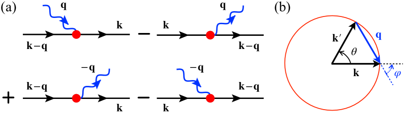
Let us first consider the problem of the non-spin-flip part of electron-magnon scattering in (49). Since scattering channels for different magnon branches are additive and electrons of opposite spin do not mix, interaction Hamiltonian can be written in a more general form that is identical to that of electron-phonon coupling
| (112) |
in which the coupling depends only on the bosonic momentum because of the adiabatic principle, , where is a phonon (magnon) Debye energy.
Collision integral for the scattering (112), schematically represented in Fig. 13(a), has a general form
| (113) | ||||
where and . Since bosons are in equilibrium, , linearization of (113) gives
| (114) | ||||
The physically justified shortcut from (114) to the relaxation-time form (110) capitalizes on the adiabatic approximation. It advocates an impurity-like, quasi-elastic picture of the scattering of the “fast” electrons on the “slow” bosons [55], which should adhere to the relaxation-time form by construction. In this case, bosonic thermal population plays the role of the thermally-excited “impurity” concentration. The resultant transport relaxation rate yields qualitatively correct answers for the resistivity of a metal due to phonon scattering in both low- and high-temperature limits, the Bloch-Grüneisen and Ohm’s laws, respectively.
Technically, this approach amounts to neglecting in the energy conservation in (114), which is indeed well-justified, and neglecting everything but in the innermost brackets of the collision integral in Eq. (114). It is the last step that is substantially harder to defend. While advanced monographs such as Ref. [59] offer a significantly more refined path that we partially follow, there are still additional constructs in it that seem unnecessary.
C.2.1 Ansatz and solution
A more intelligent way of dealing with the collision integral in (114) is to reflect on the ultimate form of that follows from the LBE (109) and from the definition of the current in (108). This suggests an ansatz
| (115) |
which adheres to the linear-response level of consideration, , and respects the reflection anti-symmetry of that follows from (108). It also explicitly separates the part of the LBE solution (109) that is strongly peaked near the Fermi energy, , from the slowly varying . By construction, the last quantity, , has the meaning of the relaxation time and is an even function of . Last but not the least, in (115) we also use continuum-like approximations for electrons, which implies spherical (circular) Fermi surface and allows us to replace with , a move that makes the subsequent steps more straightforward.
We also note that since the dependence of the equilibrium distribution functions on the momentum is only via the energy, and , there is an effective separation of variables in the ansatz (115). This is because the singular component of the ansatz, , depends sensitively on the differences due to scattering near the Fermi energy, but not on the direction of the momentum . At the same time, the factor in (115) is solely responsible for the directional dependence of , but is largely insensitive to the variations in energy due to scattering, as is argued next.
A significant simplification follows from the hierarchy of energy scales, . Since conducting electrons are confined to a proximity of the Fermi energy, the energy conservation with an emission or absorption of a boson imply a quasi-elastic nature of the scattering process, , in a full accord with the qualitative logic outlined above. The implication of this result is , valid with the accuracy . Thus, while one should keep small differences in the singular component of , it is only the direction of the momentum that can be changing significantly. This makes geometry of the scattering in Fig. 13(b) particularly simple and allows to rewrite -functions in (114) as
| (116) |
where is the angle of with , see Fig. 13(b).
The second important implication of this consideration is for the relation of to . Using (115), we write
| (117) |
As is discussed already, and is a slowly varying even function of . Since , it is natural to assume . Consider Fig. 13(b). One can break into components along and perpendicular to
| (118) |
with the latter component being odd with respect to the mirror reflection, . Making a reasonable assumption that and magnon energies are only weakly dependent on the direction of , it is easy to see that the rest of the integrand in (114) is even under the mirror reflection. Physically, the component of the contribution of a scattered state to the collision integral is identically canceled by its mirror-pair.
Thus, up to a factor and a shift of energy in from to , the non-vanishing contribution of to (114) can be written as
| (119) |
where we have converted to using the trigonometry of Fig. 13(b). Combining (115), (116), and (119), transforms collision integral in (114) to
| (120) | ||||
with
| (121) | ||||
where we used shorthand notations and with and and an identity
| (122) |
For the sake of the subsequent discussion of the spin-flip scattering that involves fewer terms in the collision integral, we note that the first (last) two lines in (121) correspond to the first (second) lines in the bracket in (114) and Fig. 13(a).
While Eq. (121) seems cumbersome and not intuitive, we will demonstrate that it is, in fact, equivalent to a compact and substantially more physical expression (127), which, upon an appropriate linearization, will yield both the proof of the approximation for the collision integral and the sought-after transport relaxation rate (130).
We note that the advocated approach of using ansatz of (115) and further manipulations with it are not unfamiliar to the experts, see Refs. [59, 73, 74]. However, they typically resort to an additional integration of both sides of the LBE (109) over electronic energy in order to eliminate the singular component that is strongly peaked near the Fermi energy. Below we demonstrate that such an ad hoc step is unnecessary.
First reorganization in (121) is an “extraction” of the bosonic distribution function that makes explicit the dependence of the scattering on the boson population
| (123) |
which, together with a “trade-off of ,”
| (124) |
reduces (121) to
| (125) |
Last is a “bosonization” of the double-fermionic terms
| (126) |
that leads to the final form
| (127) |
where the naturally-occurring factor differentiates transport scattering rate from the conventional one. The bracket in (127) can now be expanded
| (128) |
to yield the singular part of . Combining (127) and (128), we rewrite collision integral (120)
| (129) | ||||
in the long-pursued relaxation-time form (110), which naturally replicates ansatz (115) highlighted with the square bracket, also yielding transport relaxation rate
| (130) | ||||
where we have used . We also point out that a comparison of the LBE (109) with the collision integral in (129) makes explicit the equivalence of the auxiliary function from the ansatz (115) with the transport relaxation time in (130).
One can easily check by power-counting that for the scattering on acoustic phonons (, ), the relaxation rate (130) yields Ohm’s law, , for and Bloch-Grüneisen’s law, in 3D, for .
We also note that while the provided consideration is for a spherical (circular) Fermi surface, there is no question in our mind that the results concerning validity of the -approximation remain correct in general. The main modification in the relaxation rate (130) should be expected in the constraint on the surface of integration (contour in 2D), dictated by the actual shape of the Fermi surface. Thus, one can expect the results obtained using this approximation to be quantitatively correct.
C.2.2 2D case
In the present study, magnons are 2D and the relaxation rate (130) is given by an integral along a circular 1D contour in Fig. 13(b) of the radius with the magnon momentum varying from 0 to . Assuming that is less than the size of the full BZ, one can make further progress and simplify (130) by an appropriate parametrization. Let us first rewrite the summation over the BZ in (130) as an integral in polar coordinates
| (131) |
where we have abbreviated part of the integrand as
| (132) |
and is the 2D volume of the triangular-lattice BZ in Fig. 5.
Introducing new variables and and using the mirror symmetry of with respect to simplifies (131) to
| (133) |
with the momentum belonging to the 1D contour given by the parametrization . Finally, Eq. (130) transforms to
| (134) |
with from (132), , and we have explicitly separated a factor of two for the sake of combining this relaxation rate result with the one due to the spin-flip scattering processes, discussed next.
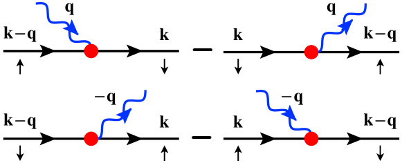
C.3 Spin-flip scattering
The spin-flip component of electron-magnon scattering in (49) generally contains two parts, one with emission by spin-down and one by spin-up electrons, yielding scattering rates that have the same structure and are additive. Therefore, we consider only one of them and write the interaction Hamiltonian in a general form that is identical to that of electron-magnon coupling in a ferromagnet
| (135) |
Here, similarly to Eq. (112), the coupling depends only on because of its local (Kondo) nature.
Owing to its relevance to the electron-magnon scattering mechanism of the resistivity in ferromagnets, the kinetic theory for the model (135) has been the subject of a number of works [73, 74, 75, 76], which, while yielding correct results, have also used unnecessary ad hoc integrations.
The principal difference of the problem from the spin-conserving scattering is in having two Boltzmann equations, one per spin projection, with their collision integrals each containing only half of the terms of (113),
| (136) | ||||
with the energy -functions as in the first and second rows of (113), respectively, see also Fig. 14, as before. Linearization in (136) gives
| (137) | ||||
We follow the narrative of the non-spin-flip consideration, with the ansatzes for as in (115)
| (138) |
and with the same continuum-like approximation for electrons. In the present case, it is also important to recall that the equilibrium distribution functions depend on the momentum and spin only via energy, , so that and .
In the considered case of the field-induced effects in an otherwise spin-compensated system, the only source of the difference in the Fermi momenta for the electrons of different spin is Zeeman energy. Because , using the same consideration of the quasielastic nature of electron-magnon scattering that is given before Eq. (116), leads to and in all scattering processes regardless of the spin, keeping geometry of the scattering the same as in Fig. 13(b) and allowing us to rewrite -functions in (137) in the form of Eq. (116).
In principle, the same consideration implies with the same accuracy of and suggests that , but we will arrive to the same conclusion via a different path.
Using the logic leading to (119), we can rewrite the non-vanishing contributions of to (137) as
| (139) | ||||
Combining (138), (116), and (139), transforms collision integrals in (137) to
| (140) | ||||
with
| (141) | ||||
where and .
The same sequence of manipulations as in (123), (124), and (126) reduce Eq. (141) identically to
| (142) | ||||
which, in a retrospect, shows that the two groups of terms in the non-spin-flip consideration (121) and Fig. 13, associated with two different energy -functions, can be reduced to a compact form (127) individually.
Linearization in the last brackets in (142) yields
| (143) |
where we note the factor of two difference with the result of an equivalent step in (128). Bringing together (142) and (143) transforms collision integrals in (140) to
| (144) |
where and and are auxiliary functions. Given the symmetry of (144) under , one can anticipate the following result. The easiest way to proceed is to realize that the content of the square bracket in the collision integrals in (144) is exactly the left-hand side of their corresponding LBEs. Substitution of (144) into LBEs with a cancellation in both sides reduces them to the two identical equations
| (145) |
which finally gives and provides the relaxation rate for both spin projections in the form
| (146) | ||||
where we note an extra factor compared to (130).
Further adaptation to the 2D case with spins on a triangular lattice considered in the preceding section gives the same result as in (134)
| (147) |
up to a factor of two that can be traced to the expansion in (128) and (143), and, ultimately, to the fact that the spin-flip scattering in (135) involves only half the terms of the non-spin-flip one in (112) for each spin species. Here is given by
| (148) |
C.4 Quasiparticle , angular dependence
Our consideration of the transport relaxation rate due to magnon scattering would not be complete without a brief note on the “regular,” or quasiparticle, relaxation rate and an equally brief remark of the relationship between the two. In turn, this analysis also allows us to discuss the angular dependence of the quasiparticle relaxation rate, originating from the discrete lattice symmetry that is encoded in the energies of spin excitations and matrix elements of the coupling to them, while leaving a substantially more involved study of their effect on its transport counterpart to a future work.
C.4.1 Quasiparticle vs transport
The quasiparticle relaxation rate characterizes a probability of the scattering of an electron from the momentum- state. It is given by
| (149) |
where is the on-shell electron self-energy.
The phonon-like non-spin-flip scattering of the form (112) yields a well-known answer for via a standard second-order diagrammatic treatment [77]
| (150) | ||||
where and as before.
While looking deceitfully different from its transport counterpart in (120), simple manipulations using (124) and (126) bring the combinations of the distribution functions in the first and second terms of (150) to
| (151) |
respectively. Recognizing the denominator in (151) for and expanding the numerators in gives
| (152) |
where we have also neglected in the delta-function. Further simplification of the latter for the spherical (cylindrical) Fermi surface (116) and parametrization of the electron mass the with energy used above, brings the quasiparticle relaxation rate in (152) close to an expression of its transport version (130)
| (153) | ||||
As is expected, the only difference between the two rates is an extra factor in the integrand of the transport relaxation rate that is responsible for the suppression of the small-angle scattering in it; as before, and are the angles between and and and , respectively, see Fig. 13(b).
Using the same approximations as in Appendix C.2 and considering the case of 2D, the quasiparticle relaxation rate (153) at reduces to
| (154) |
with from (132), , and the difference from the transport rate in (134) given by an extra factor in the latter. Needless to say, for the spin-flip scattering (135), an equivalent of the self-energy in (150) contains only half the terms, resulting in an extra factor 1/2 in (153) and (154), identically to the transport case (146) and (147) considered in Appendix C.3.
While the technical tricks of converting standard expression for the quasiparticle relaxation rate (150) into the form that is akin to the transport one (153) may not be well-known, the resultant similarity between them is in a full accord with the textbook expectations. Thus, it is prudent on our side to investigate the resulting difference between the two rates for our problem with the actual electron-magnon couplings and energies using Eqs. (51)-(53) and their quasiparticle analogues.
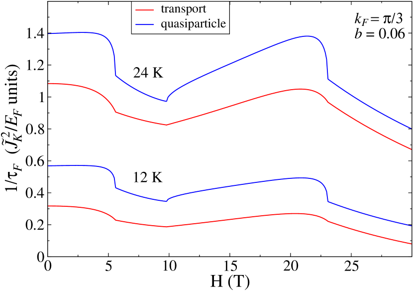
The result of such a comparison is presented in Fig. 15 for a representative value of and . The transport rates reproduce the results shown in Fig. 10(a). Although the overall field-dependence of the rates is quite similar, the quasiparticle exhibits more pronounced variations from phase to phase, with an exception of the polarized FM region, which shows only a modest overall offset from the transport one.
The evolution of with the biquadratic exchange reveals more dramatic differences. Upon approaching the first-order transition, , the Y-UUD and V-FM phase boundaries in become sharper, turning into discontinuities at . Further increase to suggest truly divergent relaxation rates to occur at the (metastable) boundaries discussed in Appendix A. This is in contrast with the evolution of the transport relaxation rate, which remains continuous at these phase boundaries up to and develops finite discontinuities for , as is demonstrated in Figs. 10(a) and (b), respectively.
Since the difference of the rates is in the suppression of the small-angle scattering in the transport case, the small-momentum contribution to the quasiparticle rate is an obvious culprit for such a dichotomy. Detailed analysis reveals the key role of the non-spin-flip scattering, present in the noncollinear Y and V phases, in precipitating singular behavior of .
In the proximity of the transitions, , where the Goldstone mode softens to , see Fig. 6, these processes provide a dangerous term to the small-momentum equivalent of the kernel (54), resulting in the leading contribution to that scales as . From Appendix A, for , still giving a continuous behavior of vs , as is shown in Fig. 15. However, for , the field-dependence of the angle switches to , resulting in a finite contribution to at and culminating in a discontinuity. Further increase to leaves the angle finite at the transition field , see Fig. 12(b), producing a true singularity, .
This discussion opens up an interesting possibility of the studies of the field-tuned singular behavior in the scattering rate due to small-angle scattering processes that can lead to a number of observables including catastrophic violation of the Wiedemann-Franz law.
C.4.2 Angular dependence of
Another aspect of the quasiparticle relaxation rate makes its consideration worthwhile. The diagrammatics-derived expression for it in Eq. (150) is exact to the second order in the coupling. The approximations leading to (152) involves only a highly-justified energy hierarchy, . The next step, resulting in (153), is a fairly reasonable assumption of the spherical (cylindrical) Fermi surface. However, this last assumption does not automatically make independent of the direction of the momentum on the Fermi surface. It is an additional step of assuming an even mirror-symmetry of the entire kernel with respect to a reflection of the momentum about the direction of the momentum which does that, leading to the final expression (154), see the line preceding Eq. (133).
Although this assumption is valid for along the high-symmetry directions, dictated by the symmetry of the triangular lattice in our case, the angular-dependence of the quasiparticle relaxation rate, encoded in the energies of spin excitations and matrix elements of the coupling to them, should remain.
A proper consideration of this problem for the transport relaxation rate has an additional complicating factor because it also requires a consistency in the assumption of the angle-dependence in relating scattered-state distribution function to , thus modifying Eq. (119). However, the simplicity of this problem for the quasiparticle relaxation rate makes it particularly appealing to solve. Thus, we return to the relaxation rate in Eq. (153) and advance it one step further to include such an angular-dependence properly, leaving its study in the transport counterpart to a future work.
Although the direction of the electron momentum is not explicitly present in (153), it is implicitly tied to that of the magnon momentum via the mutual angle , see the scattering diagram in the right inset of Fig. 16. This Figure shows that in the reference frame formed by , where is the axis perpendicular to the unit vector , the magnon momentum is parametrized as . However, this frame itself is rotated by the angle with respect to the laboratory reference frame, represented here by , with the axis tied to one of the bond-directions of the triangular lattice. Then, straightforwardly, momentum parametrization in the reference frame is .
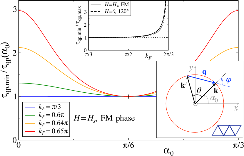
Since the absolute value of the momentum is tied to the angle via , the integral in (153) can still be reduced to a 1D form
| (155) |
where with
| (156) | ||||
We note that Eq. (155) does not have any additional approximations beyond the ones already present at the step (153). Ignoring , using symmetry of to , and introducing brings (155) back to (154). Obviously, the same considerations can be used to obtain the spin-flip equivalent of (155).
With this result (155), we can study the effect of the angular dependence of the quasiparticle relaxation rate. The findings for the polarized FM phase at the saturation field and for the 120 state as representative points of our analysis are summarized in Fig. 16. In Fig. 16 we used the same model parameters as in the rest of the paper when applied to EuC6, see Table 1, and investigated the angle-dependence of as a function of , with very similar results in both cases.
As is discussed in Sec. V for the transport case, the overall rates grow with . Since we are interested in the angular dependence, but not the absolute values, the main panel in Fig. 16 shows the quasiparticle relaxation rate from (155) as a function of normalized to its minimum value, which is in the middle of the two principal (bond) directions of the triangular lattice, denoted as . The results are shown for the FM phase and for several values of . The upper inset shows the ratio of the rates at the maximum () and minimum () vs for both FM and 120 states.
One can see that the effect of the angle-dependence in is really negligible up to about and is still very modest up to , justifying our initial approximation that neglected it and confirming the correctness of our results presented throughout the main body of the paper. In a sense, the effect is reminiscent of the accuracy of the sextupole field as nearly circular away from the close vicinity of the poles.
However, upon approaching the value of , the rates for the principal directions diverge while the rates at stay finite. As is discussed in Sec. V, this effect is due to a singularity associated with the scattering by the gapless Goldstone magnons with and equivalent ordering vectors matching for the momenta in the principal directions. In that sense, the and directions of the electron momentum for become close analogues of the “hot” and “cold” spots for the scattering, familiar from the cuprate superconductors [60]. As is mentioned above, while the same behavior is expected to occur for the transport scattering rates, the derivation of it becomes more complicated as one needs to account for the angular dependence in relating non-equilibrium distribution functions for different directions self-consistently.
References
- Abbott [2015] E. A. Abbott, Flatland (Princeton University Press, 2015).
- Novoselov [2011] K. S. Novoselov, Nobel Lecture: Graphene: Materials in the Flatland, Rev. Mod. Phys. 83, 837 (2011).
- Geim and MacDonald [2007] A. K. Geim and A. H. MacDonald, Graphene: Exploring carbon flatland, Physics Today 60, 35 (2007).
- Castro Neto et al. [2009] A. H. Castro Neto, F. Guinea, N. M. R. Peres, K. S. Novoselov, and A. K. Geim, The electronic properties of graphene, Rev. Mod. Phys. 81, 109 (2009).
- Geim and Grigorieva [2013] A. K. Geim and I. V. Grigorieva, Van der Waals heterostructures, Nature 499, 419 (2013).
- MacDonald [2019] A. H. MacDonald, Trend: Bilayer graphene’s wicked, twisted road, Physics 12, 12 (2019).
- Burch et al. [2018] K. S. Burch, D. Mandrus, and J.-G. Park, Magnetism in two-dimensional van der Waals materials, Nature 563, 47 (2018).
- Park [2016] J.-G. Park, Opportunities and challenges of 2D magnetic van der Waals materials: magnetic graphene?, Journal of Physics: Condensed Matter 28, 301001 (2016).
- Klein et al. [2018] D. R. Klein, D. MacNeill, J. L. Lado, D. Soriano, E. Navarro-Moratalla, K. Watanabe, T. Taniguchi, S. Manni, P. Canfield, J. Fernández-Rossier, and P. Jarillo-Herrero, Probing magnetism in 2d van der waals crystalline insulators via electron tunneling, Science 360, 1218 (2018).
- Gong and Zhang [2019] C. Gong and X. Zhang, Two-dimensional magnetic crystals and emergent heterostructure devices, Science 363, 10.1126/science.aav4450 (2019).
- Zhang et al. [2021] M. Zhang, Q. Hu, C. Hua, M. Cheng, Z. Liu, S. Song, F. Wang, P. He, G.-H. Cao, Z.-A. Xu, Y. Lu, J. Yang, and Y. Zheng, Metamagnetic transitions in few-layer crocl controlled by magnetic anisotropy flipping (2021), arXiv:2108.02825 [cond-mat.str-el] .
- Schafhaeutl [1840] C. Schafhaeutl, Ueber die Verbindungen des Kohlenstoffes mit Silicium, Eisen und anderen Metallen, welche die verschiedenen Gallungen von Roheisen, Stahl und Schmiedeeisen bilden, Journal für Praktische Chemie 21, 129 (1840).
- [13] Sesame Street TV series, Mr. Between, also with a symbolic appearance of Mr. Ontopof.
- Dresselhaus and Dresselhaus [1981] M. S. Dresselhaus and G. Dresselhaus, Intercalation compounds of graphite, Advances in Physics 30, 139 (1981).
- Dresselhaus [1988] M. Dresselhaus, New trends in intercalation compounds, Materials Science and Engineering: B 1, 259 (1988).
- Dresselhaus et al. [1992] G. Dresselhaus, J. T. Nicholls, and M. S. Dresselhaus, in Graphite Intercalation Compounds II: Transport and Electronic Properties, edited by H. Zabel and S. A. Solin (Springer-Verlag, Berlin, Heidelberg, 1992) Chap. Magnetic Intercalation Compounds of Graphite, p. 247.
- Enoki et al. [2003] T. Enoki, M. Suzuki, and M. Endo, Graphite Intercalation Compounds and Applications (Oxford University Press, 2003).
- Chen et al. [1986] S. T. Chen, M. S. Dresselhaus, G. Dresselhaus, H. Suematsu, H. Minemoto, K. Ohmatsu, and Y. Yosida, Magnetoresistivity and Monte Carlo studies of magnetic phase transitions in C6Eu, Phys. Rev. B 34, 423 (1986).
- Suematsu et al. [1981] H. Suematsu, K. Ohmatsu, K. Sugiyama, T. Sakakibara, M. Motokawa, and M. Date, High field magnetization of europium-graphite intercalation compound C6Eu, Solid State Communications 40, 241 (1981).
- Chubukov and Golosov [1991] A. V. Chubukov and D. I. Golosov, Quantum theory of an antiferromagnet on a triangular lattice in a magnetic field, Journal of Physics: Condensed Matter 3, 69 (1991).
- Sakakibara and Date [1984] T. Sakakibara and M. Date, Magnetism of C6Eu. I. Existence of the four-spin exchange interactions, Journal of the Physical Society of Japan 53, 3599 (1984).
- Suematsu et al. [1983] H. Suematsu, K. Ohmatsu, T. Sakakibara, M. Date, and M. Suzuki, Magnetic properties of europium-graphite intercalation compound C6Eu, Synthetic Metals 8, 23 (1983).
- Date et al. [1983] M. Date, T. Sakakibara, K. Sugiyama, and H. Suematsu, in High Field Magnetism, edited by M. Date (North-Holland, 1983) Chap. Four-spin exchange in graphite intercalation compound EuC6, p. 41.
- Sugihara et al. [1985] K. Sugihara, S. T. Chen, and G. Dresselhaus, Theory of electrical resistivity, magnetoresistance and magnon drag effect in graphite intercalation compound C6Eu, Synthetic Metals 12, 383 (1985).
- Mak et al. [2019] K. F. Mak, J. Shan, and D. C. Ralph, Probing and controlling magnetic states in 2d layered magnetic materials, Nature Reviews Physics 1, 646 (2019).
- Bud’ko et al. [2004] S. L. Bud’ko, E. Morosan, and P. C. Canfield, Magnetic field induced non-fermi-liquid behavior in YbAgGe single crystals, Phys. Rev. B 69, 014415 (2004).
- Perry et al. [2004] R. S. Perry, K. Kitagawa, S. A. Grigera, R. A. Borzi, A. P. Mackenzie, K. Ishida, and Y. Maeno, Multiple first-order metamagnetic transitions and quantum oscillations in ultrapure Sr3Ru2O7, Phys. Rev. Lett. 92, 166602 (2004).
- Jaime et al. [2002] M. Jaime, K. H. Kim, G. Jorge, S. McCall, and J. A. Mydosh, High magnetic field studies of the hidden order transition in URu2Si2, Phys. Rev. Lett. 89, 287201 (2002).
- Thomas et al. [2016] S. M. Thomas, P. F. S. Rosa, S. B. Lee, S. A. Parameswaran, Z. Fisk, and J. Xia, Hall effect anomaly and low-temperature metamagnetism in the kondo compound CeAgBi2, Phys. Rev. B 93, 075149 (2016).
- Lamura et al. [2012] G. Lamura, T. Shiroka, S. Cahen, H. Rida, N. Emery, J.-F. Marîché, P. Lagrange, and C. Hérold, The zero-field magnetic ground state of EuC6 investigated by muon spectroscopy, Carbon 50, 3995 (2012).
- Molodtsov et al. [1996] S. L. Molodtsov, C. Laubschat, M. Richter, T. Gantz, and A. M. Shikin, Electronic structure of Eu and Yb graphite intercalation compounds, Phys. Rev. B 53, 16621 (1996).
- Mashhadi et al. [2019] S. Mashhadi, Y. Kim, J. Kim, D. Weber, T. Taniguchi, K. Watanabe, N. Park, B. Lotsch, J. H. Smet, M. Burghard, and K. Kern, Spin-split band hybridization in graphene proximitized with -RuCl3 nanosheets, Nano Letters 19, 4659 (2019).
- Leeb et al. [2021] V. Leeb, K. Polyudov, S. Mashhadi, S. Biswas, R. Valentí, M. Burghard, and J. Knolle, Anomalous Quantum Oscillations in a Heterostructure of Graphene on a Proximate Quantum Spin Liquid, Phys. Rev. Lett. 126, 097201 (2021).
- Wu et al. [2021] S. Wu, Z. Xu, S. C. Haley, S. F. Weber, A. Acharya, E. Maniv, Y. Qiu, A. A. Aczel, J. B. Neaton, J. G. Analytis, and R. J. Birgeneau, Highly tunable magnetic phases in transition metal dichalcogenide Fe1/3+δNbS2 (2021), arXiv:2106.01341 [cond-mat.mtrl-sci] .
- Fan et al. [2017] S. Fan, I. Manuel, A. al Wahish, K. R. O’Neal, K. A. Smith, C. J. Won, J. W. Kim, S.-W. Cheong, J. T. Haraldsen, and J. L. Musfeldt, Electronic chirality in the metallic ferromagnet , Phys. Rev. B 96, 205119 (2017).
- Kumar et al. [2021] A. Kumar, N. C. Hu, A. H. MacDonald, and A. C. Potter, Gate-tunable heavy fermion quantum criticality in a moiré Kondo lattice (2021), arXiv:2110.11962 [cond-mat.str-el] .
- El Makrini et al. [1980] M. El Makrini, D. Guérard, P. Lagrange, and A. Hérold, Intercalation of rare earth metals in graphite, Physica B+C 99, 481 (1980).
- Rida et al. [2010] H. Rida, S. Cahen, C. Hérold, and P. Lagrange, Bulk synthesis and crystal structure of the first stage europium-graphite intercalation compound, Carbon 48, 3190 (2010).
- Yamamoto et al. [2014] D. Yamamoto, G. Marmorini, and I. Danshita, Quantum phase diagram of the triangular-lattice model in a magnetic field, Phys. Rev. Lett. 112, 127203 (2014).
- Alicea et al. [2009] J. Alicea, A. V. Chubukov, and O. A. Starykh, Quantum stabilization of the -magnetization plateau in Cs2CuCl4, Phys. Rev. Lett. 102, 137201 (2009).
- Starykh [2015] O. A. Starykh, Unusual ordered phases of highly frustrated magnets: a review, Reports on Progress in Physics 78, 052502 (2015).
- Ye and Chubukov [2017] M. Ye and A. V. Chubukov, Quantum phase transitions in the Heisenberg triangular antiferromagnet in a magnetic field, Phys. Rev. B 95, 014425 (2017).
- [43] Wolfram MathWorld, Cubic formula, https://mathworld.wolfram.com/CubicFormula.html.
- Susuki et al. [2013] T. Susuki, N. Kurita, T. Tanaka, H. Nojiri, A. Matsuo, K. Kindo, and H. Tanaka, Magnetization process and collective excitations in the triangular-lattice heisenberg antiferromagnet , Phys. Rev. Lett. 110, 267201 (2013).
- Enjalran and Gingras [2004] M. Enjalran and M. J. P. Gingras, Theory of paramagnetic scattering in highly frustrated magnets with long-range dipole-dipole interactions: The case of the pyrochlore antiferromagnet, Phys. Rev. B 70, 174426 (2004).
- Yasuda et al. [2006] C. Yasuda, D. Kinouchi, and K. Kubo, Spin-wave theory of the multiple-spin exchange model on a triangular lattice in a magnetic field: 3-sublattice structures, Journal of the Physical Society of Japan 75, 104705 (2006), https://doi.org/10.1143/JPSJ.75.104705 .
- Seki and Yunoki [2020] K. Seki and S. Yunoki, Thermodynamic properties of an ring-exchange model on the triangular lattice, Phys. Rev. B 101, 235115 (2020).
- Coletta et al. [2013] T. Coletta, M. E. Zhitomirsky, and F. Mila, Quantum stabilization of classically unstable plateau structures, Phys. Rev. B 87, 060407 (2013).
- Colpa [1978] J. H. P. Colpa, Diagonalization of the quadratic boson Hamiltonian, Physica A: Statistical Mechanics and its Applications 93, 327 (1978).
- Maldonado [1993] O. Maldonado, On the Bogoliubov transformation for quadratic boson observables, Journal of Mathematical Physics 34, 5016 (1993).
- Batyev and Braginskii [1984] É. G. Batyev and L. S. Braginskii, Antiferrornagnet in a strong magnetic field: analogy with Bose gas, JETP 60, 781 (1984).
- Zapf et al. [2014] V. Zapf, M. Jaime, and C. D. Batista, Bose-Einstein condensation in quantum magnets, Rev. Mod. Phys. 86, 563 (2014).
- Wirtz and Rubio [2004] L. Wirtz and A. Rubio, The phonon dispersion of graphite revisited, Solid State Communications 131, 141 (2004).
- Araujo et al. [2012] P. T. Araujo, M. Terrones, and M. S. Dresselhaus, Defects and impurities in graphene-like materials, Materials Today 15, 98 (2012).
- Ziman [1972] J. Ziman, Principles of the Theory of Solids (Cambridge University Press, 1972).
- Ambrosi et al. [2012] A. Ambrosi, C. K. Chua, B. Khezri, Z. Sofer, R. D. Webster, and M. Pumera, Chemically reduced graphene contains inherent metallic impurities present in parent natural and synthetic graphite, Proceedings of the National Academy of Sciences 109, 12899 (2012), https://www.pnas.org/content/109/32/12899.full.pdf .
- Esquinazi et al. [2002] P. Esquinazi, A. Setzer, R. Höhne, C. Semmelhack, Y. Kopelevich, D. Spemann, T. Butz, B. Kohlstrunk, and M. Lösche, Ferromagnetism in oriented graphite samples, Phys. Rev. B 66, 024429 (2002).
- Marder [2010] M. P. Marder, Condensed matter physics (John Wiley and Sons, Inc., 2010).
- Ziman [1963] J. M. Ziman, Electrons and Phonons (Clarendon Press, Oxford, 1963).
- Abanov et al. [2003] A. Abanov, A. V. Chubukov, and J. Schmalian, Quantum-critical theory of the spin-fermion model and its application to cuprates: Normal state analysis, Advances in Physics 52, 119 (2003).
- Osheroff et al. [1980] D. D. Osheroff, M. C. Cross, and D. S. Fisher, Nuclear Antiferromagnetic Resonance in Solid , Phys. Rev. Lett. 44, 792 (1980).
- Takahashi [1977] M. Takahashi, Half-filled Hubbard model at low temperature, Journal of Physics C: Solid State Physics 10, 1289 (1977).
- Gardner et al. [2010] J. S. Gardner, M. J. P. Gingras, and J. E. Greedan, Magnetic pyrochlore oxides, Rev. Mod. Phys. 82, 53 (2010).
- Wollny et al. [2011] A. Wollny, L. Fritz, and M. Vojta, Fractional impurity moments in two-dimensional noncollinear magnets, Phys. Rev. Lett. 107, 137204 (2011).
- Wollny et al. [2012] A. Wollny, E. C. Andrade, and M. Vojta, Singular field response and singular screening of vacancies in antiferromagnets, Phys. Rev. Lett. 109, 177203 (2012).
- Brenig and Chernyshev [2013] W. Brenig and A. L. Chernyshev, Highly dispersive scattering from defects in noncollinear magnets, Phys. Rev. Lett. 110, 157203 (2013).
- Park et al. [2021] P. Park, K. Park, J. Oh, K. H. Lee, J. C. Leiner, H. Sim, T. Kim, J. Jeong, K. C. Rule, K. Kamazawa, K. Iida, T. G. Perring, H. Woo, S.-W. Cheong, M. E. Zhitomirsky, A. L. Chernyshev, and J.-G. Park, Spin texture induced by non-magnetic doping and spin dynamics in 2D triangular lattice antiferromagnet h-Y(Mn,Al)O3, Nature Communications 12, 2306 (2021).
- Chubukov and Jolicoeur [1992] A. V. Chubukov and T. Jolicoeur, Order-from-disorder phenomena in heisenberg antiferromagnets on a triangular lattice, Phys. Rev. B 46, 11137 (1992).
- Jolicoeur et al. [1990] T. Jolicoeur, E. Dagotto, E. Gagliano, and S. Bacci, Ground-state properties of the Heisenberg antiferromagnet on a triangular lattice, Phys. Rev. B 42, 4800 (1990).
- Chernyshev and Zhitomirsky [2006] A. L. Chernyshev and M. E. Zhitomirsky, Magnon decay in noncollinear quantum antiferromagnets, Phys. Rev. Lett. 97, 207202 (2006).
- Chernyshev and Zhitomirsky [2009] A. L. Chernyshev and M. E. Zhitomirsky, Spin waves in a triangular lattice antiferromagnet: Decays, spectrum renormalization, and singularities, Phys. Rev. B 79, 144416 (2009).
- Ivanov [1993] N. B. Ivanov, Spin-wave results for the triangular antiferromagnet with next-nearest-neighbor couplings, Phys. Rev. B 47, 9105 (1993).
- Mannari [1959] I. Mannari, Electrical Resistance of Ferromagnetic Metals, Progress of Theoretical Physics 22, 335 (1959).
- Mills and Lederer [1966] D. Mills and P. Lederer, The contribution of s-d exchange scattering to the electrical resistivity of magnetic metals, Journal of Physics and Chemistry of Solids 27, 1805 (1966).
- Turov [1955] E. A. Turov, Electrical conductivity of ferromagnetic metals at low temperatures, Izv. Akad. Nauk USSR, ser. fiz. 19, 474 (1955).
- Vonsovskii and Izyumov [1963] S. V. Vonsovskii and Y. A. Izyumov, Electron theory of transition metals, II, Physics-Uspekhi 5, 723 (1963).
- Mahan [2000] G. D. Mahan, Many-Particle Physics (Springer, Boston, MA, 2000).