Spin precession of binary neutron stars with magnetic dipole moments

Abstract

Spin precession equations including the spin-orbit (SO), spin-spin (SS), quadrupole-monopole (QM) and magnetic dipole-magnetic dipole (DD) leading-order interactions are derived for compact binary systems in order to investigate the DD contribution in the orbit-averaged spin precession equations for binary neutron star systems neglecting the gravitational radiation-reaction effect. It is known that the magnitudes of spins are not conserved quantities due to the DD interaction. We give a simple analytical description for the pure DD interaction making the magnitudes of spins almost constant by neglecting the SO, SS and QM contributions. We also demonstrate the evolutions of the relative angles of spins and magnetic dipoles with the help of numeric simulations including all contributions (SO, SS, QM and DD) and introduce a dimensionless magnetic dipole parameter to characterize the strength of magnetic fields for some realistic neutron star binaries. We find that for realistic configurations the strong magnetic fields of neutron stars can modify the spin dynamics over long periods of time.

I Introduction

Nowadays, spinning astrophysical objects have come to the forefront in particular through the detection of gravitational waves (GWs). The most important targets of GW detectors are binaries of neutron stars (NS) and/or black holes (BH) [1, 2, 3, 4, 5, 6, 7, 8]. Numerous independent astronomical observations have also confirmed that spins of objects are not negligible, e.g., spin magnitude can be as high as $0.9$ in case of the recently discovered supermassive M87 BH [9]. Several studies have shown the spin of a BH to be commonly close to $1$, which is the case of an extremal Kerr BH [10]. The maximum spin value of a NS is $0.7$ for a wide class of realistic equations of state [11]. But the realistic spin of a NS is rather small, for instance, the fastest known pulsar in a binary NS system, J0737-3039A has a value of $0.03$. In the process of GW searches there is a non-trivial loss in signal-to-noise ratio if the maximum spin value is restricted to be less than $0.05$ [12]. Numerical studies have shown that in the case of a minor residual spin of $10^{-4}$ the evolution of spinning NS binaries indicates that their spin precession can be well described by post-Newtonian approximation [13].

Consideration of spins $\mathbf{S_{i}}$ of bodies in physical systems leads to spin precession equations (SPEs) which are important for the investigation of classical and/or quantum systems. The first analytical solution of SPEs averaged over one orbital period (ASPEs) has been given for compact binaries containing the leading-order spin-orbit (SO) interaction and the leading-order radiation-reaction contribution only [14]. They have presented the transitional and the simple precession movements of the orbital plane due to spin dynamics for two equivalent cases, which are the equal mass and the single spin configurations. Further interpretations and applications of this approach were given for spin-flip and spin flip-flop effects [16]. ASPEs with spin-spin (SS) contributions taking into account gravitational radiation were also analytically solved for the case of equal mass and equal spin magnitude [17].

It is important to note that in case of BHs [18] ASPEs can be integrated by adding the quadrupole-monopole (QM) terms, where the dimensionless quadrupole parameters $a_{i}$ are equal to $1$ [19]. In this case there is a new conserved quantity $\xi$ on which many further spin precession analytical solutions are built [20, 21, 22, 23, 24]. It is also important to mention that if the quadrupole parameters are not equal to $1$ ($a_{i}\neq 1$), i.e., in the case of NSs, this $\xi$ scalar is not a conserved quantity.

Solution of the instantaneous SPEs with SO, SS and QM terms for arbitrary quadrupole parameters was given by perturbative methods [25], where the motion of the polar and azimuthal angles can be completely separated. It is interesting to note that the SPEs do not depend on the spin supplementary conditions (SSC), while the radial and angular motion and waveforms are SSC-dependent in case of a compact binary with leading order spin-orbit interaction [26]. Equilibrium solutions of the SPEs can be found in [27]. Secular SPEs for NSs, gravastars and boson stars, where the quadrupole parameters are also not equal to 1, have been studied in [28] and their linear stability was analyzed in [29]. Recently, higher-order SPEs were also examined analyzing numerically generated gravitational waveforms and hybrid models [30].

The observed radio pulsar NSs have strong magnetic fields typically of $10^{12}$ G, while magnetars have fields of $10^{12}-10^{15}$ G. The recently discovered youngest and fastest magnetar Swift J1818.0-1607 has a magnetic field of $7\times 10^{14}$ G and a spin period of $1.36$ s [31]. Therefore it is important to examine whether the strength of this magnetic field or dipole field plays a role in spin dynamics. The Lagrangian formalism of the magnetic dipole-magnetic dipole (DD) interaction, the energy and angular momentum losses under gravitational radiation in case of circular and eccentric orbits are given in [32, 33, 34]. The generalized Kepler equation containing the DD contribution has been calculated in [35], but the DD interaction generates effects of the same magnitude as the second post-Newtonian correction, in pure relativistic terms, in magnetic fields up to $10^{16}$ G. Recently, some authors pointed out that the magnitude of the magnetic dipole moment can also be larger by order of three magnitudes for white dwarfs than for NSs [36]. They also estimated the precession rates of the magnetic moments for azimuthal angles using a model where the magnetic dipoles are aligned with the corresponding spin vectors and showed that the DD effect in GW could be important for future data processing of the Laser Interferometer Space Antenna (LISA) mission. It is worth to note that the full description of spinning binary NSs with considerable magnetospheres is given by magnetohydrodynamic (MHD) equations. Some MHD simulations demonstrated the conversion of a binary system’s kinetic energy into electromagnetic radiation through unipolar induction and accelerating magnetic dipole effects [37].

In this paper, we study the influence of the magnetic field on the conservative part of ASPEs due to DD contribution through the inspiral phase, while we do not take into account the gravitational radiation effect. In this case, the magnitudes of the spin vectors are not constants. Therefore $\xi$ will not be a conserved quantity, which means that an analytical approach similar to [18] will not work in this case. The DD contribution is usually rather small, thus it is important to investigate the long-term evolution of a binary NS system. Initially, we neglect the standard effects arising from the SO, SS and QM contributions and instead focus only on the DD interaction, which model we will call the pure DD case further on. We solve this model for a simple case, when we only consider the linear-order magnetic dipole terms. The validity of this model is examined by numerical developments. Next, we numerically examine the solution of the total ASPEs with all contributing terms (SO, SS, QM, and DD) included. We demonstrate the time evolution of relative spin angles through the inspiral phase for several binary NS systems with realistic spin and magnetic dipole ratios (Table 1). Furthermore, we present some cases for which it is important to take into account the magnetic dipoles of binary NSs.

The paper is organized as follows. In Section 2 we introduce the SPEs containing the SO, SS, QM and DD contributions. In Section 3 we study the pure DD model in SPEs neglecting the SO, SS and QM interactions. We compare the perturbative solutions of the pure DD model with the exact numeric solutions and present the limits of applicability for the perturbative method in this case. In Section 4 the discussion of the SPEs, containing all contributions, based on various numerical examples is presented and Section 5 contains the conclusion.

Throughout the paper we use the geometric unit system in which $G=c=\mu_{0}=1$, where $G$ is the gravitational constant, $c$ is the speed of light and $\mu_{0}$ is the vacuum permeability ($\mu_{0}=4\pi\times 10^{-7}$ Tm/A in SI units), but we kept the SI units in Table 1. We will not use the Einstein convention thus there is no summation for repeated indices. The overhat symbol above a vector represents the unit vector notation, e.g., for any vector $\mathbf{A}$ then $\mathbf{\hat{A}=A/}A$ is the unit vector, where $A=\left|\mathbf{A}\right|$ is the magnitude of $\mathbf{A}$.

II Spin precession equations

We consider a binary NS system where the characteristics of the individual objects are their masses $m_{i}$, mass moments of inertia $\mathcal{I}_{i}$, quadrupole parameters $a_{i}$, spin vectors $\mathbf{S_{i}}$ and magnetic dipole moments $\mathbf{d}_{\mathbf{i}}$ (see Fig. 1). The radial motion and gravitational radiation effects of the DD interaction can be found in [32, 33, 34]. We review the conservative part of the orbit-averaged SPE system without radiation-reaction contributions, which are given by [14, 33, 18]

$$\mathbf{\dot{S}_{1}} = \frac{1}{2r^{3}}\Bigl{\{}\left(4+3\nu_{1}\right)\mathbf{L_{N}\times\mathbf{\mathbf{S_{1}}}+S_{2}\times\mathbf{S_{1}}}$$ (1)

$$-3\left[\mathbf{\hat{L}_{N}\cdot S_{2}}+a_{1}\nu_{1}(\mathbf{\hat{L}_{N}\cdot S_{1}})\right](\mathbf{\hat{L}_{N}\times\mathbf{S_{1})}}$$

$$\ \mathbf{+d}_{2}\times\mathbf{d_{1}+}3(\mathbf{d}_{2}\mathbf{\cdot\hat{L}}_{\mathbf{N}})(\mathbf{\hat{L}}_{\mathbf{N}}\times\mathbf{d_{1})}\Bigr{\}}\ ,$$

$$\mathbf{\dot{S}_{2}} = \frac{1}{2r^{3}}\Bigl{\{}\left(4+3\nu_{2}\right)\mathbf{L_{N}\times\mathbf{S_{2}}+S_{1}\times\mathbf{S_{2}}}$$ (2)

$$\mathbf{\mathbf{-}}3\left[\mathbf{\hat{L}_{N}\cdot S_{1}}+a_{2}\nu_{2}(\mathbf{\hat{L}_{N}\cdot S_{2}})\right](\mathbf{\hat{L}_{N}\times\mathbf{S_{2})}}$$

$$\mathbf{+d}_{1}\times\mathbf{d_{2}+}3(\mathbf{d}_{1}\mathbf{\cdot\hat{L}}_{\mathbf{N}})(\mathbf{\hat{L}}_{\mathbf{N}}\times\mathbf{d_{2})}\Bigr{\}}\ ,$$

$$\mathbf{\dot{L}_{N}} = \frac{1}{2r^{3}}\Bigl{\{}(4\mathbf{S}+3\bm{\sigma})\times\mathbf{L_{N}}$$ (3)

$$\mathbf{-}3\left[(\mathbf{\hat{L}}_{\mathbf{N}}\mathbf{\cdot S}_{\mathbf{2}})\mathbf{S}_{\mathbf{1}}+(\mathbf{\hat{L}}_{\mathbf{N}}\mathbf{\cdot S}_{\mathbf{1}})\mathbf{S}_{\mathbf{2}}\right]\times\mathbf{\hat{L}}_{\mathbf{N}}$$

$$+{3}\sum_{i=1}^{2}a_{i}\nu_{i}(\mathbf{\hat{L}}_{\mathbf{N}}\mathbf{\cdot S_{i}})(\mathbf{\hat{L}}_{\mathbf{N}}\mathbf{\times\mathbf{S_{i})}}$$

$$\mathbf{\mathbf{+}}3\sum_{i\neq j}^{2}\mathbf{(d_{i}\cdot\hat{L}_{N})(d_{j}\times\hat{L}_{N}})\Bigr{\}}\ ,$$

$$\mathbf{\dot{d}_{i}} = \frac{1}{\mathcal{I}_{i}}\mathbf{S}_{\mathbf{i}}\times\mathbf{d_{i}}\ ,$$ (4)

where the overdot represents differentiation with respect to time, $r=a(1-e^{2})^{1/2}$ is the orbit-averaged diameter, $a$ is the semimajor axis and $e$ is the eccentricity (for further details see [38]). In addition, $r$ can also be considered as the radius of the circular orbit (e.g., in [14]). The Newtonian orbital momentum is $\mathbf{L_{N}=}\mu\mathbf{r\times v}$, where $\mu=m_{1}m_{2}/(m_{1}+m_{2})$ is the reduced mass, $\mathbf{r}$ is the relative position vector and $\mathbf{v}$ is the relative velocity. The unit vector of $\mathbf{L_{N}}$ is $\mathbf{\hat{L}_{N}=L_{N}/}L_{N}$, where $L_{N}=\left|\mathbf{L_{N}}\right|$ is the magnitude of $\mathbf{L_{N}}$. Furthermore, the shorthand notations are $\nu_{1}=m_{2}/m_{1}$, $\nu_{2}=m_{1}/m_{2}$, $\mathbf{S=S}_{\mathbf{1}}+\mathbf{S}_{\mathbf{2}}$ and $\bm{\sigma=}\nu_{1}\mathbf{S}_{\mathbf{1}}+\nu_{2}\mathbf{S}_{\mathbf{2}}$. There is no summation for repeated indices $i$ in Eq. (4).

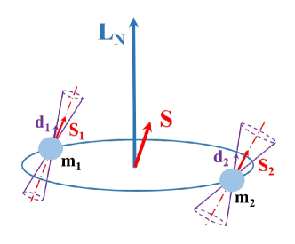
Figure 1: Geometry of a binary NS. The orbital plane is determined by the Newtonian orbital momentum $\mathbf{L_{N}}$. The characteristics of the individual NSs are their masses $m_{i}$, spins $\mathbf{S_{i}}$ and magnetic dipole moments $\mathbf{d_{i}}$.

The linear terms of spins in equation system Eqs. (1-3) are the SO contributions. The QM terms are proportional to the quadrupole parameter $a_{i}$ and are quadratic in spin, while the other quadratic-in-spin terms are the SS interactions. Obviously, the DD terms in SPEs are proportional to the product of dipole moments and the evolution equations of dipole moments are represented by Eq. (4).

The conserved quantities in general case are the total angular momentum vector $\mathbf{J=L_{N}+S}$ (here we neglect the spin-orbit angular momentum term $\mathbf{L}_{\mathbf{SO}}$ and higher order post-Newtonian contributions), the magnitude of the Newtonian angular momentum $L_{N}$ and the magnitudes of the magnetic dipole moments $d_{i}$. The magnitudes of spin vectors $S_{i\text{ }}=\left|\mathbf{S}_{\mathbf{i}}\right|$ are not conserved quantities and from Eqs. (1,2)

$$\dot{S}_{1} = \frac{d_{1}d_{2}}{2r^{3}}(\mathbf{\hat{d}_{1}}\times\mathbf{\hat{S}_{1})\cdot}\left[\mathbf{\hat{d}_{2}+}3(\mathbf{\hat{d}_{2}\cdot\hat{L}}_{\mathbf{N}})\mathbf{\hat{L}}_{\mathbf{N}}\right],$$ (5)

$$\dot{S}_{2} = \frac{d_{1}d_{2}}{2r^{3}}(\mathbf{\hat{d}_{2}}\times\mathbf{\hat{S}_{2})\cdot}\left[\mathbf{\hat{d}_{1}+}3(\mathbf{\hat{d}_{1}\cdot\hat{L}}_{\mathbf{N}})\mathbf{\hat{L}}_{\mathbf{N}}\right],$$ (6)

where we used the unit vector notations of $\mathbf{\hat{S}_{i}=S}_{\mathbf{i}}/S_{i}$ and $\mathbf{\hat{d}_{i}=}$ $\mathbf{d_{i}/}d_{i}$ with magnitude of the dipole moments $d_{i}=\left|\mathbf{d_{i}}\right|$. It can be seen that the time evolutions of magnitudes of individual spins are rather small $\dot{S}_{i}\approx\mathcal{O}(d_{1}d_{2}/r^{3})$, but they can have a significant effect in the long-term evolution of NSs.

The $\xi=\mathbf{L_{N}}\cdot\bm{(S+\sigma)}/|\mathbf{L_{N}}|^{2}$ quantity, which is conserved for the SO, SS and QM contributions, is not a conserved quantity due to the DD contribution, because in this case

$$\dot{\xi} \propto {3}\nu_{1}\left(a_{1}\mathbf{-}1\right)(\mathbf{\hat{L}}_{\mathbf{N}}\mathbf{\cdot S}_{\mathbf{1}})(\mathbf{\mathbf{\mathbf{S_{1}}}}\times\mathbf{S}_{\mathbf{2}})\mathbf{\cdot\mathbf{\hat{L}}_{\mathbf{N}}}$$ (7)

$$\mathbf{+}3\nu_{2}\left(a_{2}\mathbf{-}1\right)(\mathbf{\hat{L}}_{\mathbf{N}}\mathbf{\cdot S}_{\mathbf{2}})(\mathbf{\mathbf{\mathbf{S_{2}}}}\times\mathbf{S}_{\mathbf{1}})\mathbf{\cdot\hat{L}}_{\mathbf{N}}$$

$$\mathbf{\mathbf{-}}6\mathbf{(d_{1}\cdot\hat{L}_{N})(\hat{L}_{N}\times d_{2}})\mathbf{\cdot\mathbf{\bm{(S+\sigma)}}}$$

$$\mathbf{\mathbf{-}}6\mathbf{(d_{2}\cdot\hat{L}_{N})(\hat{L}_{N}\times d_{1}})\mathbf{\cdot\mathbf{\bm{(S+\sigma)}}}$$

$$\mathbf{-}2\nu_{1}\left(\mathbf{d}_{2}\times\mathbf{d_{1}}\right)\mathbf{\cdot L_{N}\mathbf{-}}2\nu_{2}\mathbf{\left(\mathbf{d}_{1}\times\mathbf{d_{2}}\right)\cdot L_{N},}$$

which will only be zero if

$$a_{i} = 1\text{ (for BHs) \& }m_{1}\!=\!m_{2}\text{ \& }\mathcal{O}\mathbf{(}Sd^{2})\mathbf{\approx}0,$$ (8)

$$a_{i} \neq 1\text{ (for NSs) \& }m_{1}\!=\!m_{2}\text{ \& }\mathcal{O}\mathbf{(}S^{3},Sd^{2})\mathbf{\approx}0,$$ (9)

$$a_{i} \neq 1\text{ (for NSs) \& }m_{1}\!\neq\!m_{2}\text{ \& }\mathcal{O}\mathbf{(}S^{3},Sd^{2},d^{2})\mathbf{\approx}0.$$ (10)

It is worth to note that the last condition in (8) can also be satisfied by adding an other quantity $\xi_{S^{2}}=\mathbf{S_{1}\cdot S_{2}}+\mathbf{S_{1}^{2}/}2\mathbf{+S_{2}^{2}/}2$ to $\xi$ and then the modified scalar $\xi+\xi_{S^{2}}$ will be a conserved quantity for equal-mass BHs ($a_{i}=1$ and $m_{1}=m_{2}$). The system of equations in Eqs. (1-3) cannot be solved by the analytical method used in [18] even if we neglect the changes in the $\xi$ quantity ($\dot{\xi}\mathbf{\approx}0$), since magnetic dipole vectors result in complicated coupling with spin vectors. This system of equations in Eqs. (1-3) has 9 degrees of freedom and integration of these equations is rather complicated. Therefore we neglect the SO, SS and QM terms, which we shall discuss in the next subsection.

Physical parameters	J0737-3039A	J0737-3039B	B1913+16	J1930-1852	J1906+0746	J1755-2550
Masses, $m_{1}$, $m_{2}$ [$M_{\odot}$]	1.338,1.249	1.249,1.338	1.438,1.390	<1.25,>1.30	1.291,1.322	-,>0.40
Spin frequency, $\Omega$ (Hz)	44.054	0.361	16.949	5.405	6.944	3.175
Surface magnetic field strength, $B$ [$\times 10^{5}$ T]	6.4	1590	22.8	58.5	1730	886
Mass moment of inertia, $\mathcal{I}$ [$\times 10^{38}$ kgm2]	1.064	0.994	1.144	0.994	1.027	0.318
Magnitude of spin, $S$ [$\times 10^{39}$ kgm2/s]	4.689	0.036	1.939	0.538	0.713	0.101
Magnitude of magn. dip. mom., $d$ [$\times 10^{26}$ Am2]	0.021	5.30	0.076	0.195	5.766	2.953
Spin parameter, $\chi$ [$\times 10^{-4}$]	29.75	0.26	10.65	3.91	4.86	7.17
Magnetic dipole parameter, $\chi^{d}$ [$\times 10^{-4}$]	0.006	0.160	0.002	0.01	10.16	0.862
Ratio, $\Delta=\chi^{d}/\chi$ [$\times 10^{-2}$]	0.02	60.8	0.02	0.1	3.3	12.0

Table 1: Measured and derived parameters for some binary NS systems. The observed masses, spin frequencies and surface magnetic fields are from the literature [39]. When calculating the mass moment of inertia $\mathcal{I}$, we considered the NS to be a regular sphere, so $\mathcal{I}=\frac{2}{5}mR^{2}$ with the typical radii of $R=10$ km. Magnitudes of the spin and magnetic dipole moment are derived from the $S=\mathcal{I}\Omega$ and $d=VB/\mu_{0}$ equations, respectively, where $V$ is the volume of the sphere and $\mu_{0}=4\pi\times 10^{-7}$ Tm/A is the vacuum permeability. The dimensionless spin and magnetic dipole parameters in SI units are $\chi=cS/m^{2}G$ and $\chi^{d}=\mu_{0}^{1/2}c^{2}d/m^{2}G^{3/2}$, respectively.

III Pure DD case

First, we consider the DD interactions only in the SPEs in Eqs. (1-4)  by dropping the SO, SS and QM contributions, which is called the pure DD case, as

$$\mathbf{\dot{S}_{1}} = \frac{1}{2r^{3}}\left[\mathbf{d_{2}+}3(\mathbf{d_{2}\cdot\hat{L}}_{\mathbf{N}})\mathbf{\hat{L}}_{\mathbf{N}}\right]\times\mathbf{d_{1}}\ ,$$ (11)

$$\mathbf{\dot{S}_{2}} = \frac{1}{2r^{3}}\left[\mathbf{d_{1}+}3(\mathbf{d_{1}\cdot\hat{L}}_{\mathbf{N}})\mathbf{\hat{L}}_{\mathbf{N}}\right]\times\mathbf{d_{2}}\ ,$$ (12)

$$\mathbf{\dot{L}_{N}} = \frac{3}{2r^{3}}\sum_{i\neq j}^{2}\mathbf{(d_{i}\cdot\hat{L}_{N})(d_{j}\times\hat{L}_{N}})\ ,$$ (13)

$$\mathbf{\dot{d}_{i}} = \frac{1}{\mathcal{I}_{i}}\mathbf{S}_{\mathbf{i}}\times\mathbf{d_{i}}\ .$$ (14)

It can be seen from Eqs. (11,12,14) that the scalar products of $\mathbf{\mathbf{\mathbf{S_{i}\cdot\mathbf{d}_{i}}}}$ are conserved quantities. Therefore $\frac{d}{dt}(S_{i}d_{i}\cos\alpha_{i})=0,$ where $\cos\alpha_{i}=\mathbf{\mathbf{\mathbf{\hat{S}_{i}\cdot\hat{d}_{i}}}}$ (see Fig. 2), which are not conserved quantities leading to the simple solutions of

$$\cos\alpha_{i}=\frac{C}{S_{i}},$$ (15)

where $C$ is an integration constant. It is worth to note that the polar angles $\alpha_{i}$ are conserved quantities if we drop the evolutions of the magnitudes of the spin vectors ($\dot{S}_{i}\approx 0$) in Eq. (5), in which case the magnetic dipoles would exhibit pure precessions around the individual spins.

Thus, there are 8 conserved quantities ($\mathbf{J}$, $L_{N}\,$, $d_{i}$ and $\mathbf{\mathbf{\mathbf{S_{i}\cdot\mathbf{d}_{i}}}}$) for the 15 ASPEs in Eqs. (11-14). Therefore, the pure DD system has 7 degrees of freedom.

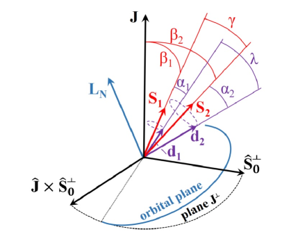
Figure 2: Geometry of a binary NS with spins and magnetic dipole moments in the coordinate system with the basis of $(\mathbf{\hat{S}_{0}^{\perp},\hat{J}}\times\mathbf{\hat{S}_{0}^{\perp},\hat{J}})$, where $\mathbf{S_{0}^{\perp}}$ is the projection of the initial total spin vector ($\mathbf{S=S_{1}}+\mathbf{S_{2}}$) onto the plane perpendicular to $\mathbf{J}$, which plane is $\mathbf{J}^{\perp}$. The nodus is the dotted line which is the intersection of the orbital plane and plane $\mathbf{J}^{\perp}$. The definitions of the introduced relative angles $\beta_{i}$, $\alpha_{i}$, $\gamma$ and $\lambda$ of $\mathbf{J}$, $\mathbf{S_{i}}$ and $\mathbf{d_{i}}$ are $\cos\beta_{i}=\mathbf{\hat{J}\cdot\hat{S}_{i}}$, $\cos\gamma=\mathbf{\hat{S}}_{\mathbf{2}}\mathbf{\cdot\hat{S}}_{\mathbf{2}},\cos\alpha_{i}=\mathbf{\hat{S}_{i}\cdot\hat{d}_{i}}$ and $\cos\lambda=\mathbf{\hat{d}_{1}\cdot\hat{d}_{2}}$. Additional definitions of polar angles, which we use in the paper, not shown in the figure, are $\cos\delta_{i}=\mathbf{\hat{J}\cdot\hat{d}_{i}}$, $\cos\varrho_{i}=\mathbf{\hat{L}}_{\mathbf{N}}\mathbf{\cdot\hat{d}_{i}}$ and $\cos\kappa_{i}=\mathbf{\hat{L}}_{\mathbf{N}}\mathbf{\cdot\hat{S}}_{\mathbf{i}}$.

III.0.1 Perturbative solution of pure DD case

In many cases, the ASPEs written in the system fixed to $\mathbf{J}$ led to an analytical solution [17, 18, 25], since $\mathbf{J}$ is a conserved quantity when the radiation-reaction effect is neglected. Therefore, in Eqs. (11,12,14), we consider the evolution equations for scalar products of $\mathbf{\hat{J}\cdot\hat{S}_{i}}$ and $\mathbf{\hat{J}\cdot\hat{d}_{i}}$ with total angular momentum unit vector $\mathbf{\hat{J}=J/}J$ and the magnitude of the total angular momentum $J=\left|\mathbf{J}\right|$ as

$$\frac{d}{dt}(\mathbf{\hat{J}\cdot\hat{S}_{1})\!} = \!\frac{d_{1}d_{2}}{2r^{3}S_{1}}\Bigl{\{}[\mathbf{\hat{d}}_{\mathbf{2}}\mathbf{+}3(\mathbf{\hat{d}}_{\mathbf{2}}\mathbf{\cdot\hat{L}}_{\mathbf{N}})\mathbf{\hat{L}}_{\mathbf{N}}]\mathbf{\cdot}[(\mathbf{\hat{d}_{1}}\times\mathbf{\hat{J})}$$ (16)

$$\!+(\mathbf{\hat{d}_{1}}\times\mathbf{\hat{S}_{1})}(\mathbf{\hat{J}\cdot\hat{S}_{1})}]\Bigr{\}},$$

$$\frac{d}{dt}(\mathbf{\hat{J}\cdot\hat{S}_{2})\!} = \!\frac{d_{1}d_{2}}{2r^{3}S_{2}}\Bigl{\{}[\mathbf{\hat{d}}_{\mathbf{1}}\mathbf{+}3(\mathbf{\hat{d}}_{\mathbf{1}}\mathbf{\cdot\hat{L}}_{\mathbf{N}})\mathbf{\hat{L}}_{\mathbf{N}}]\mathbf{\cdot[}(\mathbf{\hat{d}_{2}}\times\mathbf{\hat{J})}$$ (17)

$$\!+(\mathbf{\hat{d}_{2}}\times\mathbf{\hat{S}_{2})(\mathbf{\hat{J}\cdot\hat{S}_{2})}]}\Bigr{\}},$$

$$\frac{d}{dt}(\mathbf{\hat{J}\cdot\hat{d}_{i})\!} \mathbf{=} \mathbf{\!}\frac{S_{i}}{\mathcal{I}_{i}}(\mathbf{\hat{S}}_{\mathbf{i}}\times\mathbf{\hat{d}_{i})\cdot\hat{J}.}$$ (18)

We can compute the scalar products of $\mathbf{\hat{S}}_{\mathbf{i}}\mathbf{\cdot\hat{d}_{i}}$ from Eqs. (11) and (14) as

$$\frac{d}{dt}(\mathbf{\hat{S}}_{\mathbf{i}}\mathbf{\cdot\hat{d}_{i})}=\ \frac{d_{1}d_{2}(\mathbf{\hat{S}}_{\mathbf{i}}\mathbf{\cdot\hat{d}_{i})}}{2r^{3}S_{i}}[\mathbf{\hat{d}}_{\mathbf{j}}\mathbf{+}3(\mathbf{\hat{d}}_{\mathbf{j}}\mathbf{\cdot\hat{L}}_{\mathbf{N}})\mathbf{\hat{L}}_{\mathbf{N}}]\mathbf{\cdot}(\mathbf{\hat{d}_{i}}\times\mathbf{\hat{S}_{i})\mid}_{i\neq j},$$ (19)

where $i,j=1..2$. Assuming that the quadratic terms in magnetic dipoles can be dropped ($\mathcal{O}(d_{1}d_{2})\approx 0$) we get simple evolution equations for the pure DD case, where the introduced angles $\cos\beta_{i}=\mathbf{\hat{J}\cdot\hat{S}_{i}}$, $\cos\alpha_{i}=\mathbf{\hat{S}_{i}\cdot\hat{d}_{i}}$ (see Fig. 2) are quasi-constants

$$\frac{d}{dt}(\mathbf{\hat{J}\cdot\hat{S}_{i})} \approx 0\ ,$$ (20)

$$\frac{d}{dt}\mathbf{(\hat{S}_{i}\cdot\hat{d}_{i})} \approx 0\ ,$$ (21)

$$\frac{d}{dt}(\mathbf{\hat{J}\cdot\hat{d}_{i})} \mathbf{=} \frac{S_{i}}{\mathcal{I}_{i}}(\mathbf{\hat{S}}_{\mathbf{i}}\times\mathbf{\hat{d}_{i})\cdot\hat{J}.}$$ (22)

This system of equations can be easily integrated because from Eqs. (5,6) $\dot{S}_{i}=\mathcal{O}(d_{1}d_{2}/r^{3})\approx 0$. We transform Eq. (22) to

$$\left(\frac{d}{dt}(\mathbf{\hat{J}\cdot\hat{d}_{i})}\right)^{2} \mathbf{=} \Omega_{i}^{2}\Bigl{[}1-(\mathbf{\hat{J}\cdot\hat{S}_{i})}^{2}-\mathbf{(\hat{S}_{i}\cdot\hat{d}_{i})}^{2}-(\mathbf{\hat{J}\cdot\hat{d}_{i})}^{2}$$ (23)

$$+2(\mathbf{\hat{J}\cdot\hat{S}_{i})(\hat{S}_{i}\cdot\hat{d}_{i})}(\mathbf{\hat{J}\cdot\hat{d}_{i})}\Bigr{]}^{2},$$

where $\Omega_{i}\mathbf{=}S_{i}/\mathcal{I}_{i}$ are the spin frequencies or rotational angular velocities of NSs (e.g., see Table 1). By introducing the following relative angles of $\cos\delta_{i}=\mathbf{\hat{J}\cdot\hat{d}_{i}}$, $\cos\beta_{i0}=(\mathbf{\hat{J}\cdot\hat{S}}_{\mathbf{i}})_{0}$ and $\cos\alpha_{i0}=(\mathbf{\hat{S}}_{\mathbf{i}}\mathbf{\cdot\hat{d}_{i})}_{0}$, where angles $\alpha_{i0}$ and $\kappa_{i0}$ are quasi-constants, we get a harmonic oscillator equation in Eq. (23)

$$\frac{d^{2}\cos\delta_{i}}{dt^{2}}\mathbf{+}\Omega_{i}^{2}\cos\delta_{i}=C_{i},$$ (24)

with an introduced quasi-constant of $C_{i}=\Omega_{i}^{2}\cos\beta_{i0}\cos\alpha_{i0}$. Thus, the general solution of Eq. (24) is

$$\cos\delta_{i}=C_{i1}\cos\Omega_{i}t+C_{i2}\sin\Omega_{i}t+\frac{C_{i}}{\Omega_{i}^{2}}.$$ (25)

If we choose initial values of $\cos\delta_{i}(0)=\cos\delta_{i0}$ and $\frac{d}{dt}\cos\delta_{i}(0)=0$ then $C_{i1}=\cos\delta_{i0}-\cos\beta_{i0}\cos\alpha_{i0}$ and $C_{i2}=0$. Then we get a particular solution for Eq. (25)

$$\cos\delta_{i} = \left(\cos\delta_{i0}-\cos\beta_{i0}\cos\alpha_{i0}\right)\cos\Omega_{i}t$$ (26)

$$+\cos\beta_{i0}\cos\alpha_{i0},$$

with the initial value notations of $\cos\delta_{i0}=(\mathbf{\hat{J}\cdot\hat{d}_{i})}_{0}$, $\cos\beta_{i0}=(\mathbf{\hat{J}\cdot\hat{S}}_{\mathbf{i}})_{0}$ and $\cos\alpha_{i0}=(\mathbf{\hat{S}}_{\mathbf{i}}\mathbf{\cdot\hat{d}_{i}})_{0}$. We found that the difference between the perturbative and numerical solutions is small with a maximum difference in amplitude of $2\%$ even for large magnetic dipole parameters of $0.005$ with spin parameters of $0.001$ (see, Figs. 3 and 4).

Similar equations can be derived for the orbital angular momentum from Eqs. (13,14)

$$\frac{d}{dt}(\mathbf{\hat{L}}_{\mathbf{N}}\mathbf{\cdot\hat{d}_{i})}\mathbf{=}\frac{S_{i}}{\mathcal{I}_{i}}(\mathbf{\hat{S}}_{\mathbf{i}}\times\mathbf{\hat{d}_{i})\cdot\mathbf{\hat{L}}_{\mathbf{N}},}$$ (27)

which also leads to an oscillator equation because $\frac{d}{dt}(\mathbf{\hat{L}}_{\mathbf{N}}\mathbf{\cdot\hat{S}_{i})}\approx 0\$according to the previous approximation

$$\frac{d^{2}\cos\varrho_{i}}{dt^{2}}\mathbf{+}\Omega_{i}^{2}\cos\varrho_{i}=B_{i},$$ (28)

where $\cos\varrho_{i}=\mathbf{\hat{L}}_{\mathbf{N}}\mathbf{\cdot\hat{d}_{i}}$ and $B_{i}=\Omega_{i}^{2}\cos\kappa_{i0}\cos\alpha_{i0}$ with $\cos\kappa_{i0}=(\mathbf{\hat{L}}_{\mathbf{N}}\mathbf{\cdot\hat{S}}_{\mathbf{i}})_{0}$. Then the solution for the initial values of $\cos\varrho_{i}(0)=(\mathbf{\hat{L}}_{\mathbf{N}}\mathbf{\cdot\hat{d}_{i})}_{0}\equiv\cos\varrho_{i0}$ and $\frac{d}{dt}\cos\varrho_{i}(0)=0$  is

$$\cos\varrho_{i} = \left(\cos\varrho_{i0}-\cos\kappa_{i0}\cos\alpha_{i0}\right)\cos\Omega_{i}t$$ (29)

$$+\cos\kappa_{i0}\cos\alpha_{i0}.$$

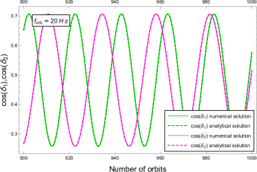
Figure 3: Evolutions of relative angles $\cos\delta_{i}$. Masses of the binary NS are $1.4M_{\odot}$ and $1.2M_{\odot}$, while the orbital frequency is $f_{orb}=20$ Hz. The dimensionless spin parameter is $\chi=0.001$ ($\chi_{1}=$ $\chi_{2}\equiv\chi$) and the ratio parameter is $\Delta$ ($=\chi^{d}/\chi=0.1$). Initial spin and dipole angles in $\mathcal{K}$ are chosen as $\theta_{1}(0)=\pi/4=\theta_{2}(0)$, $\varphi_{1}(0)=0$, $\varphi_{2}(0)=\pi/2$, $\theta_{1}^{d}(0)=\theta_{1}(0)+\pi/12=\theta_{2}^{d}(0)$, $\varphi_{1}^{d}(0)=\varphi_{1}(0)$ and $\varphi_{2}^{d}(0)=\varphi_{2}(0)$. The curves are plotted for the last $100$ orbital periods ($t_{final}=1000T_{orb}$, where $T_{orb}=1/f_{orb}$).

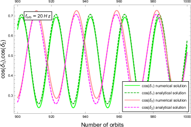
Figure 4: Evolutions of relative angles $\cos\delta_{i}$. The parameters and initial values are the same as in Fig. 3 with the exception of the ratio parameter which is $\Delta=5$. The difference between the perturbative and numerical solutions of the DD case is small with a maximum difference in amplitude of $2\%$.

III.0.2 Equal mass moments of inertia case

It can be noted that using Eq. (4) in Eqs. (5,6) we get

$$\frac{d}{dt}S_{1}^{2} = -\frac{\mathcal{I}_{1}}{r^{3}}\left[\mathbf{\mathbf{d}_{2}+}3(\mathbf{d_{2}\cdot\hat{L}}_{\mathbf{N}})\mathbf{\hat{L}}_{\mathbf{N}}\right]\mathbf{\cdot\dot{d}_{1}},$$ (30)

$$\frac{d}{dt}S_{2}^{2} = -\frac{\mathcal{I}_{2}}{r^{3}}\left[\mathbf{\mathbf{d}_{1}+}3(\mathbf{d_{1}\cdot\hat{L}}_{\mathbf{N}})\mathbf{\hat{L}}_{\mathbf{N}}\right]\mathbf{\cdot\dot{d}_{2}}.$$ (31)

If we assume equal mass moments of inertia $\mathcal{I}_{1}=\mathcal{I}_{2}\equiv\mathcal{I}$ then the summation of Eqs. (30,31) leads to a total time derivative, as

$$\frac{d}{dt}\left(S_{1}^{2}+S_{2}^{2}\right)=-\frac{\mathcal{I}}{r^{3}}\frac{d}{dt}[\mathbf{d_{1}\cdot\mathbf{d}_{2}\ +}3(\mathbf{d_{1}\cdot\hat{L}}_{\mathbf{N}})(\mathbf{\mathbf{d}_{2}\cdot\hat{L}}_{\mathbf{N}})].$$ (32)

Integrating Eq. (32) and using that $d_{i}$ are conserved quantities we get

$$S_{1}^{2}+S_{2}^{2} = -\frac{\mathcal{I}d_{1}d_{2}}{r^{3}}[\mathbf{\hat{d}_{1}\cdot\hat{d}_{2}+}3(\mathbf{\hat{d}_{1}\cdot\hat{L}}_{\mathbf{N}})(\mathbf{\hat{d}_{2}\cdot\hat{L}}_{\mathbf{N}})]+C_{0},$$

$$C_{0} = S_{10}^{2}+S_{20}^{2}$$ (33)

$$-\frac{\mathcal{I}d_{1}d_{2}}{r^{3}}[\mathbf{\hat{d}_{1}\cdot\hat{d}_{2}+}3(\mathbf{\hat{d}_{1}\cdot\hat{L}}_{\mathbf{N}})(\mathbf{\hat{d}_{2}\cdot\hat{L}}_{\mathbf{N}})]_{0},$$

where $S_{i0}$ are the initial magnitudes of spin vectors $S_{i}$ and $\left[\mathbf{...}\right]_{0}$ contains the relative angles between the initial magnetic dipole moments and the Newtonian orbital angular momentum at $t=0$. Thus, we obtain an exact relation between the magnitudes of spins and the geometry of the magnetic dipole moments for the equal mass moments of inertia case.

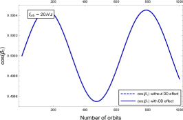
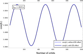
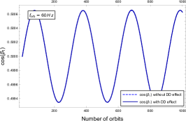
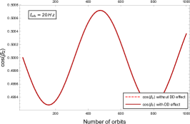
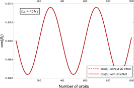
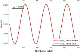
Figure 5: Evolutions of relative angles $\cos\beta_{i}=\mathbf{\hat{J}\cdot\hat{S}}_{\mathbf{i}}$. Masses of the binary NS are $1.4M_{\odot}$ and $1.2M_{\odot}$. Orbital frequencies are chosen from left to right as $20$, $40$ and $60$ Hz, respectively. The dimensionless spin parameter is $\chi=0.001$ and the ratio parameter is $\Delta=0.1$ ($=\chi^{d}/\chi$). Initial spin and dipole angles in $\mathcal{K}$ are chosen as $\theta_{1}(0)=\pi/4=\theta_{2}(0)$, $\varphi_{1}(0)=0$, $\varphi_{2}(0)=\pi/2$, $\theta_{1}^{d}(0)=\theta_{1}(0)+\pi/12=\theta_{2}^{d}(0)$, $\varphi_{1}^{d}(0)=\varphi_{1}(0)$ and $\varphi_{2}^{d}(0)=\varphi_{2}(0)$. It can be seen that the evolutions are harmonics and DD effect can be neglected in all examples.

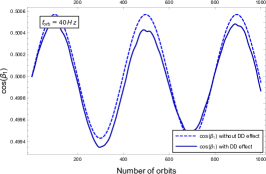
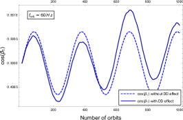
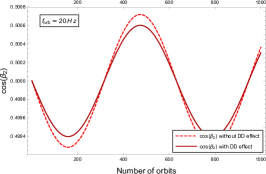
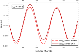
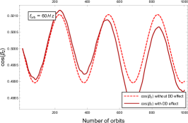
Figure 6: Evolutions of relative angles $\cos\beta_{i}$. The parameters and initial values are the same as in Fig. 5 with the exception of the ratio parameter which is $\Delta=1$ in this case. The DD effect can be seen appearing, but the difference in amplitude is rather small, $\char 126\relax 1\%$.

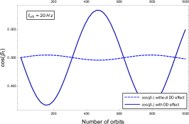
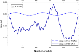
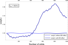
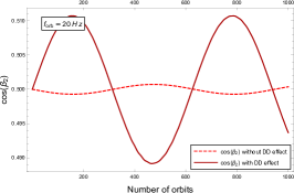
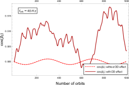
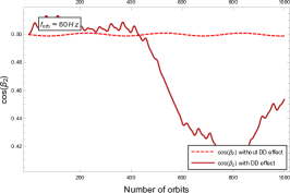
Figure 7: Evolutions of relative angles $\cos\beta_{i}$. The parameters and initial values are the same as in Fig. 5 with the exception of the ratio parameter which is $\Delta=10.$ It can be seen that the DD effect can be significant and the difference in amplitude can reach $20\%$.

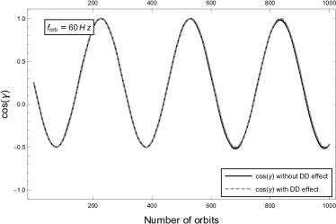
Figure 8: Evolutions of relative angle $\cos\gamma$. The parameters and initial values are the same as in Fig. 7 at orbital frequency of $60$ Hz ($\Delta=10$).

IV Numerical analysis for general case

The coupled system of first order nonlinear differential equations including the SO, SS, QM and DD terms is very complicated in Eqs. (1-4). Therefore to solve this system of equations we analyze it numerically. We will be using the dimensionless spin parameters $\chi_{i}$ and we introduce the dimensionless magnetic dipole parameters $\chi_{i}^{d}$, which are

$$\chi_{i}=\frac{cS_{i}}{Gm_{i}^{2}},\qquad\chi_{i}^{d}=\frac{\mu_{0}^{1/2}c^{2}d_{i}}{G^{3/2}m_{i}^{2}},$$ (34)

where $S_{i}$ are the magnitudes of the spin vectors, $d_{i}$ are the magnitudes of the magnetic dipole moments and $\mu_{0}=4\pi\times 10^{-7}$ Tm/A is the vacuum permeability in SI units. The magnitudes of spin vectors ($S_{i}=\mathcal{I}_{i}\Omega_{i}$, where $\mathcal{I}_{i}$ are the mass moments of inertia and $\Omega_{i}$ are the spin frequencies) and the magnitudes of magnetic dipoles $d_{i}$ appearing in these two dimensionless parameters ($\chi_{i}$ and $\chi_{i}^{d}$) can be easily calculated for each NS (see Table 1). We set $a_{i}=2$ and the radius of the NS to $10$ km in all examples below. The orbital frequencies are chosen as $20$, $40$, $60$ Hz, respectively, while the masses are set to $m_{1}=1.4M_{\odot}$ and $m_{2}=1.2M_{\odot}$, where $M_{\odot}$ is the solar mass.

In our numerical simulation we assume the dimensionless spin parameters ($\chi_{1}=$ $\chi_{2}\equiv\chi$) and the dimensionless magnetic dipole parameters ($\chi_{1}^{d}=\chi_{2}^{d}\equiv\chi^{d}$) to be equal as the companion object in a binary NS cannot always be accurately detected in astrophysics. We set the initial individual spin and magnetic dipole momentum vectors as $\mathbf{S_{i0}=}\chi_{i}\mathbf{(}\sin\theta_{i}\cos\varphi_{i},\sin\theta_{i}\sin\varphi_{i},\cos\theta_{i}$) and $\mathbf{d_{i0}=}\chi_{i}^{d}\mathbf{(}\sin\theta_{i}^{d}\cos\varphi_{i}^{d},\sin\theta_{i}^{d}\sin\varphi_{i}^{d},\cos\theta_{i}^{d}$) in the Cartesian coordinate system $\mathcal{K}=(\hat{x},\hat{y},\hat{z})$. Then, the initial spin vectors can be given in the coordinate system with the basis of $\mathcal{K}_{S}=(\mathbf{\hat{S}_{0}^{\perp},\hat{J}}\times\mathbf{\hat{S}_{0}^{\perp},\hat{J}})$, where $\mathbf{S_{0}^{\perp}}$ is the projection of the initial total spin vector onto the plane perpendicular to $\mathbf{J}$. The initial angles of $\theta_{i}$ ($\theta_{i}^{d}$) and $\varphi_{i}$ ($\varphi_{i}^{d}$) are the spherical polar angles of the spin vector in the Cartesian coordinate system $\mathcal{K}$. The transformation between $\mathcal{K}_{S}$ and the Cartesian coordinate system $\mathcal{K}$ is

$$A\mathcal{K}=\mathcal{K}_{S},$$ (35)

with the transformation matrix $A$

$$A=\left(\begin{array}[]{ccc}\frac{S_{x}}{K}&\frac{S_{y}}{K}&0\\ -\frac{S_{y}}{K}&\frac{S_{x}}{K}&0\\ 0&0&1\end{array}\right),$$ (36)

where $K=\sqrt{S^{2}-(\mathbf{S\cdot\hat{J})}^{2}}\$and $S_{x}$, $S_{y}$ are the first and second components of $\mathbf{S}$. The initial spin angles in $\mathcal{K}$ are chosen as $\theta_{1}(0)=\pi/4=\theta_{2}(0)$, $\varphi_{1}(0)=0$ and $\varphi_{2}(0)=\pi/2$. The initial magnetic dipole angles in $\mathcal{K}$ are chosen as $\theta_{1}^{d}(0)=\theta_{1}(0)+\pi/12=\theta_{2}^{d}(0)$, $\varphi_{1}^{d}(0)=\varphi_{1}(0)$ and $\varphi_{2}^{d}(0)=\varphi_{2}(0)$. The dimensionless spin parameter is $\chi=0.001$. We also introduce the ratio parameter $\Delta=$ $\chi^{d}/\chi$, which is the ratio of the dimensionless spin parameter and dimensionless magnetic dipole parameter. Usually $\Delta\ll 1$ and is rather small for NSs, but in the case of magnetars it can be large as $\Delta\simeq 10$ [31]. Thus, we investigate three cases where $\Delta=0.1,1$ and $10$ with orbital frequencies $f_{orb}=20$, $40$ and $60$ Hz. Radius $r$ in the ASPEs can be calculated from orbital frequency using Kepler’s third law as $r\equiv m^{1/3}(2\pi f_{orb})^{-2/3}$, where the total mass $m=m_{1}+m_{2}$.

We numerically studied the evolutions of $\cos\beta_{i}=\mathbf{\hat{J}\cdot\hat{S}}_{\mathbf{i}}$ for the SO, SS and QM as well as the SO, SS, QM and DD cases. Fig. 5 shows the evolutions of $\cos\beta_{i}$ for $\Delta=0.1$. It can be seen that the trajectories are simple harmonic motions, which are identical for both with and without DD effect cases. As a result, the DD interaction can be neglected for $\Delta=0.1$. The curves in Fig. 5 are plotted up to $1000$ orbits and $t_{final}=1000T_{orb}$, where $T_{orb}=1/f_{orb}$.

Fig. 6 shows the evolutions of $\cos\beta_{i}$ for $\Delta=1$, while all other initial conditions are the same as in the case of Fig. 5. The dashed lines represent the DD effect. It can be seen that the trajectories do not show simple harmonic motions from $40$ Hz upwards. The difference between the two cases (with or without DD effect) is small with a maximum difference in amplitude of $1\%$.

Fig. 7 shows the evolutions of $\cos\beta_{i}$ for $\Delta=10$. In this case the DD effect can be significant showing a $10\%$ difference in amplitude at $20$ Hz and reaching approximately a $20\%$ difference at frequencies over $40$ Hz.

Finally, we plotted the evolutions of angle $\cos\gamma=\mathbf{\hat{S}}_{\mathbf{1}}\mathbf{\cdot\hat{S}}_{\mathbf{2}}$ (Fig. 8). The DD effect does not appear throughout the evolution of this angle $\cos\gamma$, which shows simple harmonic motion for all cases.

V Conclusion

We have reviewed the leading-order orbit-averaged spin precession equations containing the SO, SS, QM and DD interactions. This differential equation system cannot be solved with the help of the scalar quantity $\xi$ introduced in [18] because it is not a conserved quantity. The pure DD case, where the SO, SS and QM contributions are neglected, can be integrated in a simple case when the evolutions of the relative $\mathbf{\hat{J}\cdot\hat{S}_{i}}$ and $\mathbf{\hat{S}_{i}\cdot\hat{d}}_{\mathbf{i}}$ angles can be dropped. This approximation can be well applied in case of short-term periods. In addition, we established a convenient relation between the magnitudes of the spins and the relative angles of the magnetic dipoles for equal mass moments of inertias.

Moreover, we have examined the full orbit-averaged spin precession equations numerically. We demonstrated several spin configurations using numerical investigations for some realistic binary NS systems. We introduced a dimensionless magnetic dipole parameter to characterize the strength of magnetic fields. Finally, we have shown that the DD effect can modify the time evolution of the spin vectors which effect is only significant in case of long periods of time and magnetars exhibiting large magnetic fields.

VI ACKNOWLEDGMENT

The work of B. M. was supported by the János Bolyai Research Scholarship of the Hungarian Academy of Sciences.

References

- [1] B. P. Abbott et al. (LIGO Scientific, Virgo), Observation of Gravitational Waves from a Binary Black Hole Merger, Phys. Rev. Lett. 116, 061102 (2016). [arXiv:1602.03837]
- [2] B. P. Abbott et al. (LIGO Scientific, Virgo), GW151226: Observation of Gravitational Waves from a 22-Solar-Mass Binary Black Hole Coalescence, Phys. Rev. Lett. 116, 241103 (2016). [arXiv:1606.04855]
- [3] B. P. Abbott et al. (LIGO Scientific, Virgo), GW170104: Observation of a 50-Solar-Mass Binary Black Hole Coalescence at Redshift 0.2, Phys. Rev. Lett. 118, 221101 (2017). [arXiv:1706.01812]
- [4] B. P. Abbott et al. (LIGO Scientific, Virgo), GW170814: A Three-Detector Observation of Gravitational Waves from a Binary Black Hole Coalescence, Phys. Rev. Lett. 119, 141101 (2017). [arXiv:1709.09660]
- [5] B. P. Abbott et al. (LIGO Scientific, Virgo), GW170817: Observation of Gravitational Waves from a Binary Neutron Star Inspiral, Phys. Rev. Lett. 119, 161101 (2017). [arXiv:1710.05832]
- [6] B. P. Abbott et al. (LIGO Scientific, Virgo), Gravitational Waves and Gamma-Rays from a Binary Neutron Star Merger: GW170817 and GRB 170817A, Astrophys. J. Lett. 848, L13 (2017). [arXiv:1710.05834]
- [7] B. P. Abbott et al. (LIGO Scientific, Virgo), GW170608: Observation of a 19 Solar-mass Binary Black Hole Coalescence, Astrophys. J. 851, L35 (2017). [arXiv:1711.05578]
- [8] B. P. Abbott et al. (LIGO Scientific, Virgo), GWTC-1: A Gravitational-Wave Transient Catalog of Compact Binary Mergers Observed by LIGO and Virgo during the First and Second Observing Runs, (2018). [arXiv:1811.12907]
- [9] F. Tamburini, B. Thide and M. D. Valle, Measurement of the spin of the M87 black hole from its observed twisted light, Mon. Not. Royal Astron. Soc. 492, L22-L27 (2020).
- [10] L. Gou, et al., The Extreme Spin of the Black Hole in Cygnus X-1, Astrophys. J. 742, 85 (2011).
- [11] K.-W. Lo and L.-M. Lin, The spin parameter of uniformly rotating compact stars, Astrophys.J. 728, 12 (2011).
- [12] D. A. Brown, I. Harry, A. Lundgren, and A. H. Nitz, Detecting binary neutron star systems with spin in advanced gravitational-wave detectors, Phys. Rev. D 86, 084017 (2012).
- [13] N. Tacik, F. Foucart, H. P. Pfeiffer, R. Haas, S. Ossokine, J. Kaplan, C. Muhlberger, M. D. Duez, L. E. Kidder, M. A. Scheel, and B. Szilágyi, Binary Neutron Stars with Arbitrary Spins in Numerical Relativity, Phys. Rev. D 92, 124012 (2015); D 94, 049903 (E) (2016).
- [14] T. A. Apostolatos, C. Cutler, G. J. Sussman, K. S. Thorne, Spin-induced orbital precession and its modulation of the gravitational waveforms from merging binaries, Phys. Rev. D 49, 6274 (1994).
- [15] L. Á. Gergely and P. L. Biermann, The spin-flip phenomenon in supermassive black hole binary mergers, Astrophys. J. 697, 1621 (2009). [arXiv:0704.1968]
- [16] C. O. Lousto, J. Healy, Flip-flopping binary black holes, Phys. Rev. Lett. 114, 141101 (2015). [arXiv:1410.3830]
- [17] T. A. Apostolatos, Influence of spin-spin coupling on inspiraling compact binaries with and , Phys. Rev. D 54, 2438 (1996).
- [18] É. Racine, Analysis of spin precession in binary black hole systems including quadrupole-monopole interaction, Phys. Rev. D 78, 044021 (2008).
- [19] E. Poisson, Gravitational waves from inspiraling compact binaries: The quadrupole-moment term, Phys. Rev. D 57, 5287 (1998).
- [20] M. Kesden, D. Gerosa, R, O’Shaughnessy, E. Berti and U. Sperhake, Effective Potentials and Morphological Transitions for Binary Black Hole Spin Precession, Phys. Rev. Lett. 114, 081103 (2015).
- [21] D. Gerosa, M. Kesden, U. Sperhake, E. Berti, and R. O’Shaughnessy, Multi-timescale analysis of phase transitions in precessing black-hole binaries, Phys. Rev. D 92, 064016 (2015).
- [22] D. Gerosa, A. Lima, E. Berti, U. Sperhake, M. Kesden and R. O’Shaughnessy, Wide precession: binary black-hole spins repeatedly oscillating from full alignment to full anti-alignment, (2018). [arXiv:1811.05979]
- [23] K. Chatziioannou, A. Klein, N. Yunes and N. Cornish Constructing gravitational waves from generic spin-precessing compact binary inspirals, Phys. Rev. D 95, 104004 (2017).
- [24] S. Khan, K. Chatziioannou, M. Hannam and F. Ohme Phenomenological model for the gravitational-wave signal from precessing binary black holes with two-spin effects, Phys. Rev. D 100, 024059 (2019).
- [25] J. Majár and B. Mikóczi, Second order spin effects in the spin precession of compact binaries, Phys. Rev. D 86, 064028 (2012).
- [26] B. Mikóczi, Spin supplementary conditions for spinning compact binaries, Phys. Rev. D 95, 064023 (2017).
- [27] J. D. Schnittman, Spin-Orbit Resonance and the Evolution of Compact Binary Systems, Phys. Rev. D 70, 124020 (2004). [arXiv:astro-ph/0409174]
- [28] Z. Keresztes, M. Tápai and L. Á. Gergely, Spin and quadrupolar effects in the secular evolution of precessing compact binaries with black hole, neutron star, gravastar, or boson star components, Phys. Rev. D 103, 084024 (2021).
- [29] Z. Keresztes and L. Á. Gergely, Stability analysis of the spin evolution fixed points in inspiraling compact binaries with black hole, neutron star, gravastar, or boson star components, Phys. Rev. D 103, 084025 (2021).
- [30] S. Akcay, R. Gamba, and S. Bernuzzi, A hybrid post-Newtonian -effective-one-body scheme for spin-precessing compact-binary waveforms up to merger, Phys. Rev. D 103, 024014 (2021).
- [31] P. Esposito et al., A Very Young Radio-loud Magnetar, Astrophys. J. Let. 896, L30 (2020).
- [32] K. Ioka and T. Taniguchi, Gravitational waves from inspiralling compact binaries with magnetic dipole moments, Astrophys. J. 537, 327 (2000).
- [33] M. Vasúth, Z. Keresztes, A. Mihály, and L. Á. Gergely, Gravitational radiation reaction in compact binary systems: Contribution of the magnetic dipole-magnetic dipole interaction, Phys. Rev. D 68, 124006 (2003).
- [34] B. Mikóczi, M Vasúth and L. Á. Gergely, Self-interaction spin effects in inspiralling compact binaries, Phys. Rev. D 71, 124043 (2005).
- [35] Z. Keresztes, B. Mikóczi and L. Á. Gergely, Kepler equation for inspiralling compact binaries, Phys. Rev. D 71, 124043 (2005).
- [36] A. Bourgoin, C. L. Poncin-Lafitte, S. Mathis, M-C. Angonin, Dipolar magnetic fields in binaries and gravitational waves, (2021), [arXiv:2109.06611].
- [37] F. Carrasco and M. Shibata, Magnetosphere of an orbiting neutron star, Phys. Rev. D101, 063017 (2020).
- [38] B. M. Barker, R. F. O’Connell, Derivation of the Equations of Motion of a Gyroscope from the Quantum Theory of Gravitation, Phys. Rev. D 2, 1428 (1970).
- [39] Modelling Double Neutron Stars: Radio and Gravitational Waves, Mon. Not. R. Astron. Soc 504, 3682 (2021).