Optical resonances in graded index spheres: A resonant-state expansion study and analytic approximations

Abstract

Recent improvements in the resonant-state expansion (RSE), focusing on the static mode contribution, have made it possible to treat transverse-magnetic (TM) modes of a spherically symmetric system with the same efficiency as their transverse-electric (TE) counterparts. We demonstrate here that the efficient inclusion of static modes in the RSE results in its quick convergence to the exact solution regardless of the static mode set used. We then apply the RSE to spherically symmetric systems with continuous radial variations of the permittivity. We show that in TM polarization, the spectral transition from whispering gallery to Fabry-Pérot modes is characterized by a peak in the mode losses and an additional mode as compared to TE polarization. Both features are explained quantitatively by the Brewster angle of the surface reflection which occurs in this frequency range. Eliminating the discontinuity at the sphere surface by using linear or quadratic profiles of the permittivity modifies this peak and increases the Fabry-Pérot mode losses, in qualitative agreement with a reduced surface reflectivity. These profiles also provide a nearly parabolic confinement for the whispering gallery modes, for which an analytical approximation using the Morse potential is presented. Both profiles result in a reduced TE-TM splitting, which is shown to be further suppressed by choosing a profile radially extending the mode fields. Based on the concepts of ray optics, phase analysis of the secular equation, and effective quantum-mechanical potential for a wave equation, we have further developed a number of useful approximations which shed light on the physical phenomena observed in the spectra of graded-index systems.

I Introduction

Modeling inhomogeneous optical resonators is challenging as generally a simple analytic solution is not available. A special case are spherically symmetric systems, having an inhomogeneity, for example in the permittivity, only dependent on the radius. Examples can be found in core-shell systems which allow highly directional scattering [LiuACSN12], when modeling surface contamination on a sphere due to diffusion [WyattPR62] or high pressure [ChowdhuryJOSAA91], or when model biological cells [HuangPRE03]. Graded index profiles can be used to engineer the cancellation of electric and magnetic dipole excitation which reduces the visibility of small particles at certain wavelengths [ShalashovTAP16]. Graded index profiles can also lead to reduced splitting between transverse-electric (TE) and transverse-magnetic (TM) modes which enhances sensitivity to chiral materials.

The scattering properties of systems with graded permittivity have been studied in the literature using various approximate methods. In the multilayer approach (also referred to as stratified medium method), the graded index profile is approximated by a piecewise constant function, describing the system by homogeneous regions comprising a core covered by a sequence of shells [WaitASRB62, KaiAO94]. In the short wavelength limit, a Debye series expansion for the scattered field was used [LockJQSRT17], and in the long wavelength limit a Born approximation [AlbiniJAP62] or a dipole limit [ShalashovTAP16] were applied to dispersive systems with complex permittivity. Furthermore, the dipole moment of dielectric spherical particles with power law radial profiles of the permittivity was calculated in the electrostatic limit [DongPRB03]. A generalized scattered field formulation developed in [WyattPR62] requires solving scalar Schrödinger-like equations, similar to the scalar wave equations solved in this work. To study the electromagnetic (EM) modes, first and second-order perturbation methods were developed [LaiPRA90] and applied to deformations of a homogeneous sphere [Leung_Pang_1996]. Whispering gallery (WG) modes in both TE and TM polarizations were studied in [ChowdhuryJOSAA91] for small inhomogeneous perturbations of the surface layer of a sphere. In that approach, the modes were found in the complex frequency plane based on the expansion coefficients of the generalized scattered field, and the secular equations were solved numerically using a Runge-Kutta method. The effect of a linearly changing permittivity profile was investigated in [IlchenkoJOSAA03] for high-frequency TE modes in large spheres, using Airy functions as an approximate solution to the corresponding scalar problem. Finally, in [LaquerbeAWPL17], a resonant mode of a sphere was treated in the electrostatic limit, for a negative and frequency dependent permittivity, described by an undamped (i.e. non-absorbing) Drude model, with radial dependencies of the permittivity and the electric field approximated by polynomials.

Here we will use the resonant-state expansion (RSE) to study the modes of graded index spherical resonators. The RSE is a rigorous theoretical method in electrodynamics for calculating the resonant states (RSs) of an arbitrary open optical system [MuljarovEPL10]. Using the RSs of a basis system, which can be chosen to be analytically solvable, such as a homogeneous dielectric sphere in vacuum, the RSE determines the RSs of the target system by diagonalizing a matrix equation containing a perturbation. This perturbation is defined as the difference between the basis and target systems and is expressed as a change of the permittivity and permeability distributions with respect to the basis system [MuljarovOL18].

For a general perturbation, one needs to include in the RSE static modes [DoostPRA14, LobanovPRA19] alongside the RSs via a Mittag-Leffler (ML) representation of the dyadic Green’s function. Note that the latter is at the heart of the RSE approach. Recently, the RSE has been reformulated [MuljarovPRA20], in order to eliminate static modes, and the illustrations provided for perturbations of the size and refractive index of a homogeneous sphere show a significantly improved convergence compared to the original version of the RSE [LobanovPRA19]. The approach [MuljarovPRA20] has also proposed, though without providing illustrations, another quickly convergent version of the RSE, the one which keeps static modes in the basis.

In this paper, we consider both versions of the reformulated RSE, with and without static modes, demonstrating a similar efficiency for both. Using the RSE, we then investigate spherically symmetric inhomogeneous systems, with graded permittivity profiles. The RSs in such systems are still split into TE and TM polarizations, and are characterized by the azimuthal ($m$) and angular ($l$) quantum numbers. Importantly, while some graded profiles are approximately solvable analytically, the RSE can treat arbitrary perturbations and finds all the RSs of the system within the spectral coverage of the basis used, thus generating a full spectrum. This allows us to identify some prominent features in spectra, such as the quasi-degeneracy of modes and the Brewster angle phenomenon, and ultimately to engineer the shape of the spectrum via changing the permittivity profile.

The paper is organized as follows. In Sec. II we study the TE and TM RSs of a homogeneous sphere, using a qualitative ray picture of light propagation and a more rigorous phase analysis of the secular equations describing the light eigenmodes, both approaches introducing several useful approximations. In Sec. III we briefly describe the RSE method and its optimizations used here for calculating the RSs of a graded index sphere. We then recap the analogy between wave optics and quantum mechanics, by introducing a radial Schrödinger-like wave equation containing an effective potential. The RSs of a sphere with linear and quadratic radial permittivity profiles eliminating the discontinuity at the sphere surface are then discussed, and an approximate analytical solution using Morse’s potential is presented. In Sec. LABEL:s:tetm_degeneracy we investigate the TE-TM RS splitting and its reduction for graded index profiles. Details of calculations are provided in Appendices, including a comparison of the performance of the two optimized versions of the RSE, with and without elimination of static modes.

II Homogeneous sphere

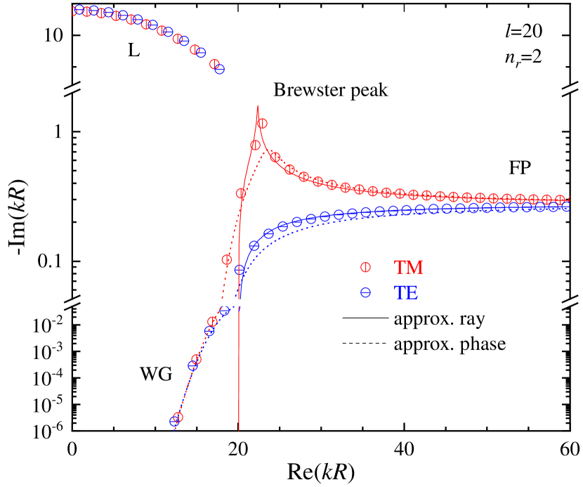
Figure 1: Wavenumbers of the TE and TM RSs of a homogeneous sphere in vacuum, with a refractive index of $n_{r}=2$ and an angular momentum quantum number of $l=20$. Solid and dashed lines are the approximations to the imaginary part of the wavenumbers, given by Eqs. (2) and (9), respectively.

Figure  1 shows the spectrum of the RSs of a homogeneous dielectric sphere in vacuum in the complex wavenumber plane, for a refractive index of the sphere of $n_{r}=2$ and an angular momentum quantum number of $l=20$. The RS wavenumbers are found by solving the secular equation, see Eq. (3) in subsection  II.2. Here, $k=\omega/c$ is the wavenumber in vacuum, $\omega$ is the light angular frequency and $c$ is the speed of light in vacuum. Only Re $k\geq 0$ is shown, noting that RSs come in pairs with both signs of the real part of their wavenumber. The spectrum consist of TE and TM modes which appear in alternating order, with one exception related to the Brewster’s angle phenomenon, as discussed below. The RSs of a sphere can be divided into three groups: leaky (L) modes, WG modes, and Fabry-Pérot (FP) modes.

Physically, all of them are formed as a results of light quantization in the system which is provided by a constructive interference of electromagnetic (EM) waves multiply reflected from the sphere surface, but this effect is more prominent for WG and FP modes.

L modes typically have very low quality factors (Q factors) and their EM fields are located mainly outside the sphere. The number of L modes is exactly $l$ in TE and $l-1$ in TM polarization, although the Brewster mode discussed later can be regarded as a hybrid L-FP mode, so that one could say that the number of L modes is effectively the same in both polarization. L modes arrange around the origin in the complex wavenumber plane, forming a roughly semicircular arc.

WG modes are formed due to the total internal reflection and therefore have wavenumbers with $|{\rm Re}\,k|<l/R$, as discussed below. The number of WG modes is increasing with $n_{r}$ and $l$. The Q factor of the fundamental WG mode is increasing exponentially with $l$, and values of up to $10^{10}$, only limited by material properties, have been demonstrated experimentally [VernooyOL98]. The EM field of the WG modes is concentrated inside the sphere close to the surface.

FP modes of a sphere have moderate Q factors and are named for their similarity to the original FP modes [PerotAJ1899] of a double-mirror planar resonator. In fact, at large frequency, the FP modes of a sphere approach the limit of an equidistant spectrum of a dielectric slab, with all the eigenfrequencies having the same imaginary part [MuljarovEPL10]. The number of FP modes is countable infinite. Their EM fields are distributed within the sphere, avoiding the centre due to the non-zero angular momentum ($l>0$). The FP modes are spectrally separated from the WG modes by the critical angle of the total internal reflection, as discussed in more depth below.

The arrangement of the RSs in Fig. 1 is overall similar in the TE and TM polarizations. The imaginary part of their wavenumbers approaches the same high frequency asymptote, albeit from opposite sides. Additionally, there is a peak in the imaginary part of the TM RS wavenumbers near the transition region from WG to FP modes, which occurs around the Brewster angle in the ray picture of light propagation, and we therefore refer to it as a Brewster peak. At this peak, an additional TM mode is formed, breaking the otherwise alternating order of TE and TM RSs.

Below we discuss and analyze the spectrum of the RSs of a sphere in more detail, using two different approaches: the ray picture and a phase analysis. Both approaches provide some useful approximations for the mode positions and linewidths and offer an intuitive understanding of the origin and properties of the RSs of a sphere.

II.1 Ray picture: Brewster’s phenomenon and total internal reflection

To understand the observation of the Brewster peak in the spectrum of the RSs, we recall that increasing the angle of light incidence $\theta$ at a planar interface between two media, the Fresnel reflection coefficient for TM (aka p) polarized light passes through zero, changing its sign at the Brewster angle [GriffithsBook17]. The same occurs at the surface of a sphere in the ray picture, which is valid in the limit of wavelengths much smaller than the surface curvature. This local geometry is illustrated in the inset of Fig. 2. The magnitude of the incident wave vector is $n_{1}k$, where $n_{1}$ is the refractive index of the corresponding medium, i.e. that the sphere, $n_{1}=n_{r}$. Since the angular momentum $l$ gives the number of wave periods along one circumference $2\pi R$, the wave vector component $p$ parallel to the surface is determined by $2\pi l=2\pi Rp$, so that $p=l/R$. With simple trigonometry we can see that $\sin\theta=p/(n_{1}k)$. The Brewster angle $\theta_{b}$ is determined by $\tan\theta_{b}=n_{2}/n_{1}$, so that for a sphere in vacuum ($n_{2}=1$) the wavenumber corresponding to the Brewster angle is given by

$$k_{b}=\frac{l}{R}\sqrt{\frac{1}{n_{1}^{2}}+1}\,.$$ (1)

At this angle, the reflectivity vanishes. This would correspond to a divergence of the imaginary part of the RS wavenumber for an ideal planar geometry. Here instead it is kept finite due to the finite curvature of the surface and the RS discretization, resulting in the Brewster peak.

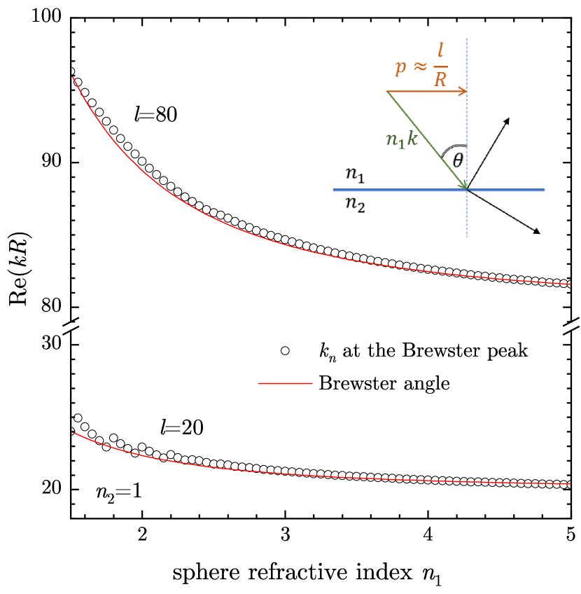
Figure 2: Real part of the wavenumber of the TM RS at the Brewster peak (circles) and function of the sphere refractive index $n_{1}=n_{r}$, for $l=20$ and $l=80$, compared with the ray optics approximation Eq. (1) (lines). Inset: sketch of the ray geometry at the boundary.

In Fig. 2 we compare Eq. (1) with the real part of the Brewster mode (the TM mode at the Brewster peak in the spectrum), for $l=20$ and $l=80$, both showing good agreement. With increasing $n_{1}$ the RSs are packed more densely in the complex $k$ plane, so that the discretization does not result in significant deviations. At the same time, the light wavelength within the sphere $2\pi/(n_{1}k)$ decreases with $n_{1}$, thus improving the validity of the ray picture.

The Brewster mode can also be associated with the leaky branch. In fact, as $n_{1}$ increases, the Brewster peak in the spectrum is getting sharper, so that the Brewster mode is taking a significantly larger imaginary part of the wavenumber compared to the neighboring FP modes and is thus getting more isolated from them, at the same time approaching the edge of the leaky branch. Indications of this can be seen in Figs. LABEL:f:sphere_app and LABEL:f:strength_perturbation in the Appendix. We also note that for high $l$, the Brewster peak can be shifted further into the FP spectral region. This happens because the Brewster angle $\theta_{b}$ is always smaller than the critical angle $\theta_{c}$ of the total internal reflection. The latter determines the point in the spectrum separating WG from FP modes and can be evaluated in a similar way, leading to $k_{c}={l}/{R}$. Comparing it with Eq. (1), we see that as $l$ increases or $n_{1}$ decreases, the difference $k_{b}-k_{c}$ is getting larger, so that the corresponding region in the spectrum, between the critical and the Brewster angles, can accommodate more RSs.

The ray picture is also useful for understanding the imaginary part of the FP mode wavenumbers. Assuming the reflectivity amplitude $r_{P}$ at the sphere surface in polarization $P$ is given by the corresponding Fresnel coefficient, we equate it to the ratio of the field amplitude before and after each reflection. This ratio is in turn given by the temporal decay of the field, $|r_{P}|=\exp(-t/\tau)$, where $t$ is the time between consecutive reflections and $\tau$ is the mode decay time which is given by the imaginary part of its eigenfrequency, $1/\tau=-\imaginary(kc)$. At the same time, the optical path length across the sphere between two reflections is given by $L=2Rn_{r}\cos\theta$. Finally, using the fact that $t=L/c$ and taking the logarithm of the reflectivity results in

$$\imaginary k=\frac{\ln|r_{P}|}{2Rn_{r}\cos\theta},$$ (2)

where the Fresnel coefficient $r_{P}$ depends on the angle of incidence $\theta$ and the refractive index of the sphere $n_{r}$. The expression is valid up to the critical angle $\theta_{c}$ of total internal reflection, at which $\ln|r_{P}|=0$. The values obtained according to Eq. (2) are shown in Fig. 1 as solid lines. We can see a good agreement for both polarizations, including the Brewster peak and the asymptotic value for FP modes, evaluated to $-0.27465/R$ for $n=2$ and $\theta=0$, which again validates the ray optics interpretation of the RS properties. The WG modes are located in the total internal reflection region of the spectrum where Eq. (2) is not applicable – their non-vanishing imaginary parts are the result of the finite curvature of the sphere making the reflection imperfect. We therefore consider in the following subsection a refined approximation (shown in Fig. 1 by dashed lines) which is based on the phase analysis of the secular equation determining the RSs.

II.2 Phase analysis: Mode positions and linewidths

The secular equation determining the RS eigen wavenumber $k_{n}$ of a non-magnetic homogeneous sphere of radius $R$ with vacuum outside is given by [MuljarovPRA20]

$$\frac{J^{\prime}(n_{r}k_{n}R)}{J(n_{r}k_{n}R)}=\frac{1}{\beta}\frac{H^{\prime}(k_{n}R)}{H(k_{n}R)},$$ (3)

where $\beta=n_{r}$ ($\beta=n_{r}^{-1}$) for TE (TM) polarization. Here $J(x)=xj_{l}(x)$ and $H(x)=xh^{(1)}_{l}(x)$, with $j_{l}$ and $h^{(1)}_{l}$ being, respectively, the spherical Bessel function and Hankel function of first kind, and primes mean the first derivatives of functions with respect to their arguments. For $|z|\gg l$, we can approximate the left hand side of Eq. (3) as [SehmiPRB20]

$$\frac{J^{\prime}(z)}{J(z)}\approx-\tan(z-\frac{l+1}{2}\pi)\,.$$ (4)

It is therefore useful to introduce the following two phase functions:

$$\Psi(k)=\atan(-\frac{J^{\prime}(n_{r}kR)}{J(n_{r}kR)})$$ (5)

and

$$\Phi(k)=\atan\left(-\frac{1}{\beta}\frac{H^{\prime}(kR)}{H(kR)}\right)\,.$$ (6)

Substituting them into Eq. (3) yields

$$\Psi(k_{n})=\Phi(k_{n})+n\pi\,,$$ (7)

where $n$ is an arbitrary integer. For real $k$, it can be seen that $\Psi(k)$ is a real monotonous function (on a selected Riemann sheet), and according to Eq. (4) becomes linear at large $k$. At the same time, $\Phi(k)$ is complex even for real $k$, and its real part varies between $\pi/2$ and 0 monotonously (non-monotonously) with $k$ for TE (TM) polarization. All three functions, $\Psi(k)-n\pi$, and Re $\Phi(k)$ for TE and TM polarizations, are plotted in Fig. LABEL:f:phase in Appendix LABEL:a:phase_analysis, which allows a graphical solution of Eq. (7). Namely, the intersections of the curves for $\Psi(k)-n\pi$ and Re $\Phi(k)$ determine the approximate positions of the modes in spectra. More rigorously, separating the real and the imaginary parts of the wavenumber, $k_{n}=k^{\prime}_{n}+ik_{n}^{\prime\prime}$, the mode positions in spectra, $k_{n}^{\prime}$, are given by

$$\Psi(k_{n}^{\prime})-n\pi\approx{\rm Re}\,\Phi(k_{n}^{\prime})\,,$$ (8)

whereas $k_{n}^{\prime\prime}$, determining the mode linewidths, by

$$k_{n}^{\prime\prime}\approx\frac{1}{n_{r}R}\,{\rm Im}\,\Phi(k_{n}^{\prime})\,,$$ (9)

in accordance with the asymptotic behaviour Eq. (4).

The approximation Eq. (9) for the mode linewidth is illustrated in Fig. 1 by dashed lines, demonstrating a good agreement for WG and FP modes. While it is less accurate than Eq. (2) for most FP modes, it provides a suited approximation for the WG modes, where the latter fails. The accuracy provided by this approximation improves as the refractive index $n_{r}$ of the sphere increases, as seen in Fig. LABEL:f:sphere_app in Appendix LABEL:a:phase_analysis. Compared to Eq. (1.1) of [LamJOSAB92], here Eq. (8) is not an explicit expression for mode position, and the approximation Eq. (9) is less accurate than Eq. (1.3) of [LamJOSAB92], but the graphical solution (Fig. LABEL:f:phase) provides intuition into the emergence of the modes and the difference between the TE and TM polarizations.

Using the above phase analysis, one can also obtain an analytic approximation for the RSs wavenumbers in the large frequency limit, $n_{r}kR\gg l$. Using the fact that $\tan\Phi(k)\to-i/\beta$ at $k\to\infty$ and the asymptotic behaviour of $\Psi(k)$ given by Eq. (4), one can evaluate

$$\begin{split}k^{\rm TE}_{n}&\approx\frac{1}{2n_{r}R}\left[(2n+l+1)\pi-i\ln{\frac{n_{r}+1}{n_{r}-1}}\right]\,,\\ k^{\rm TM}_{n}&\approx\frac{1}{2n_{r}R}\left[(2n+l+2)\pi-i\ln{\frac{n_{r}+1}{n_{r}-1}}\right]\,,\end{split}$$ (10)

where the integer $n$ can be used to number the RSs. For a full derivation of Eq. (10), see Appendix LABEL:a:phase_analysis.

The RS wavenumbers given by the approximation Eq. (10) are identical to those of a homogeneous slab at normal incidence [MuljarovEPL10]. The latter are in turn consistent with Eq. (2) used for the normal incidence reflection, which gives $\imaginary(kR)=\ln[(n_{r}-1)/(n_{r}+1)]/(2n_{r})$, as in Eq. (10). At non-normal incidence, the TE and TM FP modes of a slab asymptotically converge to each other in pairs, as shown in Fig. LABEL:f:homogeneous_slab in Appendix LABEL:a:homogeneous_slab. The planar system gives rise to both even and odd modes (using the parity of the electric or magnetic field), with odd TE modes converging to even TM modes at large frequencies, and vise versa. In the sphere, however, there are no even modes, as required by the finiteness of the EM field at the origin (as in any other point in space). Then, by removing the even modes from the slab spectra we obtain the alternating nature of the FP modes, which is exactly what we see in the analytic approximation Eq. (10) and in the spectrum of the sphere presented in Fig. 1.

III Graded index spheres

In this section we study, using the RSE, the RSs in spherically symmetric non-magnetic systems with graded permittivity profiles. A particularly interesting situation is reached by removing discontinuities of the permittivity. Here we study cases where the discontinuity is removed either only in the permittivity (linear case) or both in the permittivity and its derivative (quadratic case), and compare both cases with each other and with the constant permittivity profile studied in Sec. II. We note that removing discontinuities of the refractive index yields broadband anti-reflecting coatings in planar dielectric layers [HedayatiM16]. For the WG modes, we introduce a radial Schrödinger-like wave equation containing an effective potential, compare potentials and mode properties in all three cases, and provide an analytical approximation based on the Morse potential.

III.1 Calculating the RSs via the RSE

It is straightforward to use the RSE for calculating the RSs of a graded index sphere. The difference in the permittivity between the target system (a graded index sphere) and the basis system (a constant index sphere) is treated as a perturbation, and the RSs of the constant index sphere serve as a basis for the RSE. The EM fields of the RSs of the target system are expanded into the basis RSs, and the expansion coefficients and the RS wavenumbers of the target system are found by solving a linear eigenvalue problem, see Eq. (LABEL:RSE-gen) in Appendix LABEL:a:RSE. This eigenvalue problem of the RSE contains as input the RS wavenumbers of the basis system and the matrix elements of the perturbation. For spherically symmetric systems, TE and TM polarizations do not mix and can be treated separately in RSE as well as the RSs with different $l$ and magnetic quantum number $m$. However, the matrix elements used in the RSE for the TE and TM RSs are different, see [MuljarovPRA20] and Appendix LABEL:a:RSE for details. In particular, for TM polarization, one needs to include in the basis additional functions which are required for completeness and physically describe the part of the EM field in a graded index sphere which is not divergence free. More rigorously, these functions are required to properly describe a longitudinal part of the dyadic GF related to its static pole in the ML explansion.

Previously, this problem has been treated within the RSE by introducing a complete set of static modes [LobanovPRA19]. However, even though the treatment of static modes is numerically less complex, a slow convergence versus the basis size observed in [LobanovPRA19] remained an issue. To develop quickly converging versions of the RSE, the full ML representation of the dyadic GF of a spherically symmetric system has been studied in [MuljarovPRA20], focusing in particular on the static pole of the GF containing a $\delta$-like singularity. A quick convergence of the RSE has been achieved and demonstrated in [MuljarovPRA20] by an explicit isolation of the singularity that has allowed to avoid its direct expansion into static modes. Two ML forms of the GF have been introduced in [MuljarovPRA20], called there ML3 and ML4, which led to slightly different versions of the RSE, both quickly convergent to the exact solution.

The quick convergence of the RSE based on ML4, with static mode elimination and suited only for a basis system in a form of a homogeneous sphere, was demonstrated in [MuljarovPRA20] on examples of both size and material (strength) perturbations of a sphere. However, the version of the RSE based on ML3, which is using explicitly a static mode set and an arbitrary spherically symmetric basis system, has not been studied so far numerically. Such a study is given in Appendix LABEL:a:RSE, including a comparison with ML4, demonstrating a similar level of convergence. We show there in particular that the RSE based on ML3 and ML4 have both a quick $1/N^{3}$ convergence to the exact solution, where $N$ is the basis size of the RSE. Furthermore, taking three different static mode sets introduced earlier in [LobanovPRA19, MuljarovPRA20], we show in Appendix LABEL:a:RSE that the results of the RSE based on ML3 are similar for the different static mode sets previously suggested.

Let us finally note that for perturbations without discontinuities, the above mentioned optimization of the RSE might be not needed, as demonstrated in a similar approach based on eigen-permittivity modes [ChenJCP20]. However, as we are going to consider a transformation of an optical system from a homogeneous sphere, having a discontinuity, to a sphere with a continuous permittivity profile, the perturbation describing this transformation and used in RSE contains a discontinuity, both in linear and quadratic cases, and therefore the above optimization is in fact needed.

In all calculations of the RSs of the graded index spheres done in this paper, we use the RSE based on ML4, as it has a fixed number of additional basis functions in TM polarization, which is three times the number of the TM RSs included in the basis. We use the basis size (i.e. the total number of modes in the basis) of $N=800$ in both cases of linear and quadratic profiles.

III.2 Effective potential

To intuitively understand the properties of the RSs in graded-index optical systems, it is useful to consider the analogy between Maxwell’s and Schrödinger’s wave equations and to introduce an effective optical potential [JohnsonJOSAA93]. In spherically symmetric systems, all the components of the electric and magnetic fields can be expressed in terms of a radially dependent scalar field [MuljarovPRA20]. For TE (TM) polarization, this is the magnitude of the electric (magnetic) field, which has only a tangential component $E(r)=\mathcal{E}(r)/r$ ($H(r)=-i\mathcal{H}(r)/r$). For non-magnetic systems, with the radial permittivity profile $\varepsilon(r)$ and permeability $\mu(r)=1$, the scalar field $\mathcal{E}(r)$ satisfies the following Schrödinger-like equation [MuljarovPRA20]

$$\left(\derivative[2]{r}-\frac{\alpha^{2}}{r^{2}}+k^{2}\varepsilon(r)\right)\mathcal{E}(r)=0\,,$$ (11)

where $\alpha=\sqrt{l(l+1)}$. In fact, assuming the particle mass $M=\hbar^{2}/2$, Eq. (11) can be interpreted as a quantum-mechanical analogue (QMA). An obvious limitation of this QMA is that $k^{2}$, playing the role of the complex eigenvalue for the RSs, contributes to Eq. (11) not the same way as the energy in Schrödinger’s equation. Associating $k^{2}$ with the particle energy, and using the fact that $\varepsilon(r)=1$ (or a constant) outside the system, Johnson [JohnsonJOSAA93] introduced an energy-dependent effective potential, which makes the analogy with quantum mechanics no so straightforward. Here instead, we interpret Eq. (11) as an equation for the zero-energy state of a particle in a one-dimensional potential

$$V^{\rm TE}(r)=-k^{2}\varepsilon(r)+\frac{\alpha^{2}}{r^{2}}\,,$$ (12)

in which $k$ plays the role of a complex parameter of the potential. In this QMA, every RS of the optical system, described by the wave function $\mathcal{E}(r)$, has zero quantum-mechanical energy and potential Eq. (12) used for this single state only, characterized by an individual value of $k$.

Likewise, for TM polarization, the scalar field $\mathcal{H}(r)$ satisfies an equation [MuljarovPRA20]

$$(-\frac{1}{\epsilon (r)}$$ (13)