CC-Cert: A Probabilistic Approach to Certify General Robustness of Neural Networks

Abstract

In safety-critical machine learning applications, it is crucial to defend models against adversarial attacks — small modifications of the input that change the predictions. Besides rigorously studied $\ell_{p}$-bounded additive perturbations, semantic perturbations (e.g. rotation, translation) raise a serious concern on deploying ML systems in real-world. Therefore, it is important to provide provable guarantees for deep learning models against semantically meaningful input transformations. In this paper, we propose a new universal probabilistic certification approach based on Chernoff-Cramer bounds that can be used in general attack settings. We estimate the probability of a model to fail if the attack is sampled from a certain distribution. Our theoretical findings are supported by experimental results on different datasets.

Introduction

Deep neural network (DNN) models have achieved tremendous success in many tasks. On the other hand, it is well known that they are intriguingly susceptible to adversarial attacks of different kinds (?), thus there is a pressing lack of models that are robust to such attacks. Several mechanisms are proposed as empirical defenses to various known adversarial perturbations. However, these defenses have been later were circumvented by new more aggressive attacks (?; ?; ?; ?).

Therefore, a natural question arises: given a DNN model $f$, can we provide any provable guarantee on its prediction under a certain threat model, i.e. $f(x)=f(x_{T})$, where $x_{T}$ is a transformed input? This is precisely the topic of a growing field of certified robustness. A part of the existing research relies on the analysis of the Lipschitz properties of a classifier: its output’s Lipschitz-continuity leads to a robustness certificate for additive attacks (?; ?; ?). Another excellent tool for such a task is smoothing: the inference of the model is replaced by averaging of predictions over the set of transformed inputs. First, this approach was developed for small-norm attacks (?; ?), but then it was successfully generalized to a much more general class of transforms such as translations or rotations (?; ?). A recent work (?) and its follow-up (?) study a general smoothing framework that is able to provide useful certificates for the most common synthetic image modifications and their compositions.

However, a drawback of smoothing methods is that they can only certify a smoothed model which is significantly slower than the original one due to a large number of samples to approximate the expectation. Thus, we need a method that a) can certify any given black-box model, and b) is general and not tailored to a specific threat model (such as small-norm perturbations). Providing an exact rigorous certification in this setting is a very challenging task.

Instead, in this paper, we propose and investigate a probabilistic approach that produces robustness guarantees of a black-box model against different threat models. In this approach, we estimate the probability of misclassification, if the attack is sampled randomly from the admissible set of attacks. We bound this quantity by the probability of the large deviation of a certain random variable $Z$, which is derived from the distance between the probability vectors (see Lemma 1). To estimate the probability of the large deviation, we propose to use the empirical version of the Chernoff-Cramer bound and show that under the additional assumption on $Z$ this bound holds with high probability (see Theorem 1).

Our contributions are summarized as follows:

• We propose a new framework called Chernoff-Cramer Certification (CC-Cert) for probabilistic robustness bounds and theoretically justify them based on the empirical version of Chernoff-Cramer inequality;

• We test those bounds and demonstrate their efficacy for several models trained in different ways for single semantic parametric transformations and some of their compositions.

Preliminaries

Figure 1: Illustration of Algorithm (1) for a single sample. Classifier $f$ is used to compute vector $\mathbf{p}$ of class probabilities and the difference $d$ between its two largest components for initial sample $x$. Then, initial sample is perturbed by transformation $\mathcal{T}_{\theta}$ to obtain its $n$ perturbed versions $\{x_{T_{i}}\}_{i=1}^{n}$. Classifier $f$ is then applied to these perturbed samples to obtain corresponding probability vectors $\{\mathbf{p}_{T_{i}}\}_{i=1}^{n}$ and discrepancies $\{Z_{i}\}_{i=1}^{n}$. Next, given the discrepancies $\{Z_{i}\}_{i=1}^{n}$ and set $\mathbf{t}$ of temperatures, an empirical Chernoff bound is compute. The procedure of computation of bound is repeated $k$ times and resulting maximum bound is divided by $\delta$ in order to minimize the probability of bound obtained to be less than the actual one in Chernoff-Cramer method. Finally, the obtained quantity $\hat{b}$ is treated as an upper bound for the probability of change of classifier’s prediction under transform $\mathcal{T}_{\theta}$ of its input $x$ which is certified with probability $1-\varepsilon$ if $\hat{b}<\varepsilon$.

We consider the classification task with fixed set of data samples ${\mathcal{S}=\{(x_{1},y_{1}),\dots,(x_{m},y_{m})\}}$ where $x_{i}\in\mathbb{R}^{D}$ is a $D-$dimensional input drawn from unknown data distribution $p_{\text{data}}$ and $y_{i}\in\{1,\dots,K\}$ are corresponding labels. Let ${f:\mathbb{R}^{D}\to[0,1]^{K}}$ be the deterministic function such that ${\displaystyle h(x)=\operatorname*{\arg{}\,\max}_{k\in\{1,\dots,K\}}f_{k}(x)}$ maps any input $x$ to the corresponding data label.

Under a transformation ${T:\mathbb{R}^{D}\to\mathbb{R}^{D}}$, an input image $x$ is transformed into $x_{T}=T(x)$. It is known that $f(x)$ and $f(x_{T})$ may differ significantly under certain transformations, namely, some perturbations which do not change semantic of an image may mislead the classifier $h(\cdot)$ that correctly classifies its unperturbed version. In our work, we focus on certifying the stability of $h(\cdot)$ under transformation $T$ with certain assumptions on its parameter space $\Theta$, or, in other words, providing guarantees that $h(\cdot)$ is probabilistically robust at $x$ under perturbation of general type. A more formal description of such perturbations is given in

Definition 1.

Perturbation of general type is a parametric mapping $T:\Theta\times\mathcal{X}\to\mathcal{X}.$ Throughout the paper, we denote $\Theta$ as a parameter space of a given transform, $T_{\theta}(x)=x_{T}$ as the transformed version of $x$ given $\theta\in\Theta$ and $\mathbb{S}_{T}(x)$ as the space of all transformed versions of $x$ under perturbation $T.$

Definition 2 (Probabilistic robustness, (?)).

Let $T$ be the transformation of general type and $x$ be the input sample with ground truth class $c$. Suppose that $\mathbb{S}_{T}(x)$ is the space of all images $x_{T}$ of $x$ under perturbations induced by $T$ and $\mathbb{P}$ be the probability measure on space $\mathbb{S}_{T}(x)$. The $K$-class model $f$ is said to be robust at point $x$ with probability at least $1-\epsilon$ if

$$\mathbb{P}_{x_{T}\sim\mathbb{S}_{T}(x)}\left(\operatorname*{\arg{}\,\max}_{k\in\{1,\dots,K\}}f_{k}(x_{T})=c\right)\geq 1-\epsilon.$$ (1)

Probabilistic Certification of Robustness

Robustness and Large Deviations

Our proposal is to certify the robustness of the classifier $f$ by estimating the probability of large deviations of its output probability vectors. The following lemma shows how the discrepancy $f(x)-f(x_{T})$ between the output vectors $f(x)$ and $f(x_{T})$ assigned by $f$ to the original sample $x$ and its transformed version $x_{T}$ is connected to their predicted class labels.

Lemma 1.

Let $f:\mathbb{R}^{D}\to[0,1]^{C}$ be the classifier with a known inference procedure and $x$ be an input sample. Let $x_{T}$ be a transformation of $x$ after transform $T\in\mathcal{T}$ where $\mathcal{T}$ is a given class of transforms. Assume that ${\mathbf{p}=f(x)}$ and ${\mathbf{p}_{T}=f(x_{T})}$ are the probability vectors of the original sample $x$ and its transformed version $x_{T}$, respectively. Let ${c=\arg\max\mathbf{p}}$ and ${\tilde{c}=\arg\max\mathbf{p}_{T}}$ be the classes assigned by $f$ to $x$ and $x_{T}$, respectively and let $d=\frac{p_{1}-p_{2}}{2}$ be the half of the difference between two largest components of $\mathbf{p}.$

Then, if $\|\mathbf{p}-\mathbf{p}_{T}\|_{\infty}<d$ holds, $\tilde{c}=c$.

Proof.

Suppose that ${c\neq\tilde{c}}$, then, ${{\mathbf{p}_{T}}_{\tilde{c}}>{\mathbf{p}_{T}}_{c}}$ and ${\mathbf{p}_{c}>\mathbf{p}_{\tilde{c}}.}$ On the other hand, since the difference norm ${\|\mathbf{p}-\mathbf{p}_{T}\|_{\infty}=\max(|\mathbf{p}_{1}-\mathbf{p}_{T_{1}}|,\dots,|\mathbf{p}_{C}-{\mathbf{p}_{T}}_{C}|)<d,}$ we have

$$\mathbf{p}_{c}-d<{\mathbf{p}_{T}}_{c}\ \text{and}\ {\mathbf{p}_{T}}_{\tilde{c}}-d<\mathbf{p}_{\tilde{c}},$$

which leads to

$${\mathbf{p}_{T}}_{c}-{\mathbf{p}_{T}}_{\tilde{c}}>(\mathbf{p}_{c}-d)-(\mathbf{p}_{\tilde{c}}+d)=\mathbf{p}_{c}-\mathbf{p}_{\tilde{c}}-2d.$$

Since $2d=p_{1}-p_{2}=\mathbf{p}_{c}-p_{2},$

$$\mathbf{p}_{c}-\mathbf{p}_{\tilde{c}}-2d=p_{2}-\mathbf{p}_{\tilde{c}}\geq 0,$$

yielding a contradiction. Thus, $c=\tilde{c}.$ ∎

Intuitively, the lemma states that whenever the maximum change in the output $\mathbf{p}_{T}$ does not exceed half the distance $d$ between the two largest components in $\mathbf{p}$, the argument of the maximum in $\mathbf{p}_{T}$ does not change in comparison to the one in $\mathbf{p}$.

We suggest to estimate the right tail of the probability distribution of $Z=Z_{x,\mathcal{T}}=\|\mathbf{p}-\mathbf{p}_{T}\|_{\infty}$. Namely, we want to bound from above the probability $\mathbb{P}\left(Z\geq d\right)$ to provide guarantees that transformations from class $\mathcal{T}$ applied to $x$ do not lead to a change of class label assigned by $f.$

Deriving the Bound: Estimates of the Tail of the Distribution

In this section, we describe our method to estimate the tail of probability distribution. Namely, we refer to the Chernoff-Cramer approach and propose a technique that allows us to use a sample mean instead of the population mean in the right-hand side of the bound.

Lemma 2 (Markov’s inequality).

Let $Z$ be a non-negative scalar random variable with finite expectation and $t\in\mathbb{R},t>0$, then

$$\mathbb{P}(Z\geq t)\leq\frac{\mathbb{E}(Z)}{t}.$$

Lemma 3 (Chernoff-Cramer method, (?)).

Let $Z$ be a scalar random variable, $t\in\mathbb{R},t>0$ and $d\in\mathbb{R}$. Then

$$\mathbb{P}(Z\geq d)=\mathbb{P}(e^{Zt}\geq e^{dt})\leq\frac{\mathbb{E}(e^{Zt})}{e^{dt}}$$ (2)

by a Markov’s inequality.

The right-hand side of Eq. 2 is the upper-bound for $\epsilon$ in Eq. 1. Note that depending on the value of $t$, Eq. 2 produces a lot of bounds, so it is natural to choose $t$ that minimizes its right-hand side.

Sample Mean Instead of True Expectation.

Overall, we want to use Eq. (2) to bound the probability that the deviation between $\mathbf{p}$ and $\mathbf{p}_{T}$ is greater than half the difference between the two largest components of $\mathbf{p}$, i.e. $d$. Unfortunately, it is impractical to compute its right hand side directly, because the population mean of $e^{Zt}$ is unknown in general. Instead, the task is to estimate the density of

$$Y=\exp(-dt)\frac{1}{n}\sum_{i=1}^{n}\exp(Z_{i}t),$$ (3)

where $\forall i\in\{1,\dots n\}$ $Z_{i}=\|\mathbf{p}-\mathbf{p}_{T_{i}}\|_{\infty}$ is the norm of the difference in the probability vectors of original and transformed samples. There is a certain challenge in such an approach: when the population mean is replaced by the sample mean, it is possible to underestimate the true expectation, and thus, provide an incorrect bound which is less than the right-hand side of Eq. (2). It implies that the inequality

$$\mathbb{P}(Z\geq d)\leq Y,$$ (4)

which is the modification of (2) by the replacement of the true expectation by a sample mean, holds with some probability: it is guaranteed to hold only in case ${Y\geq e^{-dt}\mathbb{E}(e^{Zt})}.$

Thus, the probability of the sample mean to underestimate the population mean,

$$\mathbb{P}\left(Y\leq\frac{\mathbb{E}(e^{Zt})}{e^{dt}}\right),$$ (5)

needs to be small as it regulates the correctness of computation of the bound in the form of Eq. (3). Our proposal is to bound from above the probability in Eq. (5) by sampling $k$ i.i.d. sample means $\{Y_{1},\dots,Y_{k}\}$ in the form of (3) and exploit the statistics of the random variable $\max(\{Y_{1},\dots,Y_{k}\}).$

The pseudo-code in Algorithm 1 summarizes the bound computation for a single input $\mathbf{x}$.

function bound($f,\mathbf{x},y,\mathbf{t},\texttt{transform},n,k,\delta$)

     $\mathbf{p}\leftarrow f(\mathbf{x})$ $\triangleright$ compute model output on original $x$

     $d=\frac{\mathbf{p}[0]-\mathbf{p}[1]}{2}$ $\triangleright$ Compute the difference between top 2 classes

     $\hat{y}=\texttt{max}(\mathbf{p})$ $\triangleright$ compute predicted class

     $\texttt{hit}\leftarrow\hat{y}==y$ $\triangleright$ boolean variable indicating correctness of prediction for initial input

     $\mathbf{x}_{n}=\texttt{repeat}(\mathbf{x},n)$ $\triangleright$ repeat original input $n$ times

     $\mathbf{p}_{n}=\texttt{repeat}(\mathbf{p},n)$ $\triangleright$ repeat $\mathbf{p}$ $n$ times

     $\texttt{bounds}\leftarrow\{0,\dots,0\}$ $\triangleright$ initialize placeholder for bounds with $k$ zeros

     for i=0, i<k, i++ do

         $\mathbf{x}_{T}=\texttt{transform}(\mathbf{x}_{n})$ $\triangleright$ apply random transforms to input $\mathbf{x}_{n}$

         $\mathbf{p}_{T}\leftarrow f(\mathbf{x}_{T})$ $\triangleright$ compute model output on transformed $\mathbf{x}_{T}$

         $\textbf{Z}=\|\mathbf{p}_{n}-\mathbf{p}_{T}\|_{\infty}$ $\triangleright$ compute the change in output vector in terms of max norm

         $\textbf{Z}\mathbf{t}^{\top}=\texttt{outer}(\textbf{Z},\mathbf{t})$ $\triangleright$ multiply every diff by vector of temperatures $\mathbf{t}$

         $\mathbb{E}(e^{\textbf{Z}\mathbf{t}})=\texttt{mean}_{0}(\texttt{exp}(\textbf{Z}\mathbf{t}^{\top}))$ $\triangleright$ compute sample mean over $n$ random transforms

         $e^{d\textbf{t}}=\texttt{exp}(d\mathbf{t})$

         $\mathbf{b}=\mathbb{E}(e^{\textbf{Z}\mathbf{t}})/e^{d\mathbf{t}}$ $\triangleright$ get the bounds vector over temperatures

         $b_{\text{min}}=\texttt{min}(\mathbf{b})$ $\triangleright$ compute the smallest bound over temperatures

         $\texttt{bounds}[i]\leftarrow b_{\text{min}}$      

     $\texttt{bound}=\frac{1}{\delta}\texttt{max}(\texttt{bounds})$ $\triangleright$ compute the largest of obtained bounds and normalize by $\delta$

     return $\texttt{min}(1.0,\texttt{bound})$, hit

Algorithm 1 Chernoff-Cramer bound calculation algorithm.

Several Sample Means Instead of One.

In this section, we show that, under certain assumptions, bound provided by the Algorithm (1) may be used instead of the right-hand side of Eq. (2).

Lemma 4 (Paley-Zygmund, (?)).

Suppose a random variable $X$ is positive and have finite variance, $\sigma^{2}_{X}<\infty$. Then, $\forall\delta\in(0,1)$,

$$\mathbb{P}\left(X<\delta\mathbb{E}(X)\right)\leq\frac{\sigma^{2}_{X}}{\sigma^{2}_{X}+(1-\delta)^{2}(\mathbb{E}(X))^{2}}.$$ (6)

Theorem 1 (Worst-out-of-k-bounds).

Suppose that random variable $X$ takes values from $[0,1]$, probability density function of random variable $\xi=e^{Xt}$ is positively skewed and has coefficient of variation $C_{v}=\frac{\sigma_{\xi}}{\mathbb{E}(\xi)}\sim 1$. Then, given $\hat{b}$ as the bound produced by the Algorithm 1,

$$\mathbb{P}\left(\hat{b}<\frac{\mathbb{E}(\xi)}{e^{dt}}\right)<\left(\frac{1}{1+\frac{{n}(1-\delta)^{2}}{C^{2}_{v}}}\right)^{k}.$$ (7)

Proof.

As one of the steps of the Algorithm  1, sample means $Y_{j}=\overline{\xi}_{j}e^{-dt}=\left\{\frac{\sum_{i=1}^{{n}}e^{tX_{i}}}{{n}e^{dt}}\right\}_{j}$ are computed. Note that the expectation and variance of $\xi$ and $\overline{\xi}$ are related as ${\mathbb{E}(\overline{\xi})=\mathbb{E}(\xi)=\mu_{\xi}}$ and $\sigma^{2}_{\overline{\xi}}=\frac{\sigma^{2}_{\xi}}{{n}}$, respectively.

Then, according to (6),

$$\begin{split}\mathbb{P}\left(\overline{\xi}<\delta\mathbb{E}(\overline{\xi})\right)&=\mathbb{P}\left(\overline{\xi}<\delta\mu_{\xi}\right)\leq\frac{\sigma^{2}_{\overline{\xi}}}{\sigma^{2}_{\overline{\xi}}+(1-\delta)^{2}(\mu_{\xi})^{2}}\\ &=\frac{\sigma^{2}_{\xi}}{\sigma^{2}_{\xi}+{n}(1-\delta)^{2}\mu^{2}_{\xi}}=\frac{1}{1+\frac{{n}(1-\delta)^{2}}{C^{2}_{v}}}\\ &=p({n},C_{v}).\end{split}$$

Since sample means $\overline{\xi}_{j}=Y_{j}e^{dt},j\in[1,\dots,k],$ in Algorithm (1) are i.i.d.,

$$\mathbb{P}\left(\max(\overline{\xi_{1}},\dots,\overline{\xi_{k}}\right)<\delta\mu_{\xi}) =\prod_{j=1}^{k}\mathbb{P}\left(\xi_{j}<\delta\mu_{\xi}\right)$$

$$\leq\prod_{j=1}^{k}p({n},C_{v})=p({n},C_{v})^{k}.$$

Thus, since the left-hand side of the above inequality is the one from (7), namely

$$\mathbb{P}\left(\max(\overline{\xi_{1}},\dots,\overline{\xi_{k}})<\delta\mu_{\xi}\right) =\mathbb{P}\left(\frac{1}{\delta}\max(\overline{\xi_{1}},\dots,\overline{\xi_{k}})<\mu_{\xi}\right)$$

$$=\mathbb{P}\left(\hat{b}<\frac{\mathbb{E}(\xi)}{e^{dt}}\right),$$

inequality (7) holds. ∎

Remark.

When the number of samples in the Algorithm  1 is enough, namely, $n>n_{0}=(1-\delta)^{-2}C^{2}_{v},$ the right hand side of inequality (7) is less than $\left(\frac{1}{2}\right)^{k}$. In other words, there exists a number $n_{0}$ such that for all $n>n_{0}$ the probability can be made small for not very large $k$. In Figure 2, we present an example of positively skewed probability density.

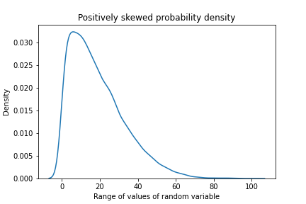
Figure 2: Example of positively skewed probability density function.

Types of Model Training and Computation Cost of Inference

It should be mentioned that our method can be applied for certification of any model $f(x)$, i.e. it does not require changing the inference procedure as it is done in smoothing methods. However, if the model training is done in the standard way, the overall robust accuracy is expected to be significantly lower than the plain accuracy of the model. A straightforward way to improve the robustness of the model is to modify the training procedure. We can adapt the training procedure used in smoothing methods such as (?). Such procedure can be implemented through data augmentation: the model is trained on transformed samples, thus we expect it will have higher robust accuracy. During the inference stage, the smoothed model has to be evaluated many times (?), thus increasing the complexity. In our approach, we can apply the certification directly to the original model trained in an augmented way. Our numerical experiments confirm that such models typically have better accuracy, however, there are notable exceptions. This means that more research is needed in training more robust plain models and/or mixed approaches such as smoothing with a small number of samples.

Experiments

In order to evaluate our method, we assess the proposed bounds on the public datasets, namely, MNIST and CIFAR-10.

All the models, training and testing procedures are implemented in PyTorch (?), and the transformations considered are implemented with use of Kornia framework (?). We use architectures, training parameters and procedures from (?) and evaluate our approach on $500$ random test samples for each experiment, following (?).

As a result of the experiments, we provide probabilistically certified accuracy, PCA, in dependence on probability threshold $\varepsilon$ and show how it is connected to empirical robust accuracy, ERA, under corresponding adaptive attack. Namely, given the classifier $h(\cdot)$, set of images ${\mathcal{S}=\{(x_{1},y_{1}),\dots,(x_{m},y_{m})\}}$ and threshold $\varepsilon$, probabilistically certified accuracy is computed as

$$\text{PCA}(\mathcal{S},\varepsilon)=\frac{\left|(x,y)\in\mathcal{S}:\texttt{BOUND}(x)<\varepsilon\ \&\ h(x)=y\right|}{m}.$$

At the same time, given the discretization ${\Theta=\{\theta_{1},\dots,\theta_{r}\}}$ of space of parameters of the transform $T$, empirical robust accuracy is computed as a fraction of objects from $\mathcal{S}$ that are correctly classified under all the transformations $T_{\theta_{i}},i\in[1,\dots,r]:$

$$\text{ERA}(\mathcal{S})=\frac{\left|(x,y)\in\mathcal{S}:h(T_{\theta_{i}}(x))=y\ \forall i\in[1,\dots r]\right|}{m}.$$

Bound Computation Parameters and Cost

In all our experiments, we use the following parameters for the Algorithm 1: number of samples ${n=200}$, number of bounds ${k=30}$, parameter ${\delta=0.9}$ for Lemma (4), temperature vector $\mathbf{t}$ consists of $500$ evenly spaced numbers from interval $[10^{-4},10^{4}]$. We use $r=20$ as discretization parameter for space of parameters for each transform. Execution of the Algorithm 1 on single GPU Tesla V100-SXM2-16GB takes ${30-1000}$ seconds on MNIST and ${60-2000}$ seconds on CIFAR-10 depending on the transform complexity.

Considered Transformations

Here we present the set of transformations studied in this work and provide the set of corresponding parameters used in the experiments with single transformations.

Image Rotation.

The transformation of rotation is parameterized by the rotation angle $\phi$ and is assumed to be followed by the bilinear interpolation with zero-padding of rotated images. In case of CIFAR-10 dataset, we use ${\Theta=\{\phi\in[-10^{\circ},10^{\circ}]\}}$, and ${\Theta=\{\phi\in[-50^{\circ},50^{\circ}]\}}$ for MNIST.

Image Translation.

The transformation of image translation is parameterized by a translation vector and is also assumed to be followed by bilinear interpolation. We use zero-padding and are not restricted to discrete translations. In case of CIFAR-10, we use $\Theta=\{v\in\mathbb{R}^{2}:|v|\leq 0.2*w\}$, and for MNIST $\Theta=\{v\in\mathbb{R}^{2}:|v|\leq 0.3*w\}$, with $w$ equal to the width/height of the image, i.e. translation by no more than $20\%$ of image for CIFAR-10 and no more than $30\%$ of image for MNIST, respectively.

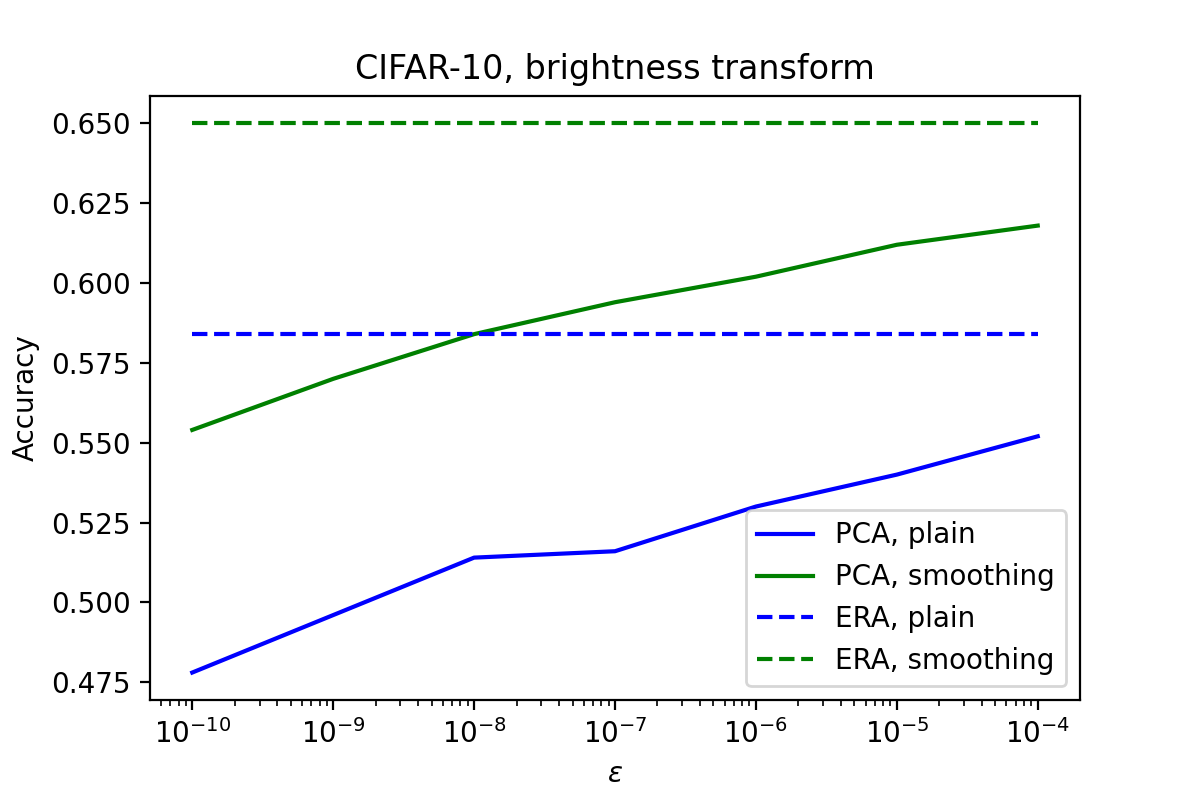
Figure 3: An illustration of the evaluation protocol on CIFAR-10 dataset, brightness adjustment transform. Number of samples ${n=20000}$, number of computed bounds ${k=30}$, ${\delta=0.9}$, brightness adjustment parameter ${\theta_{b}\in[-40\%,+40\%].}$

Brightness Adjustment.

The transformation of brightness adjustment is just an element-wise addition of a brightness factor to an image. We change the brightness by no more than $40\%$ for CIFAR-10 and by no more than $50\%$ for MNIST.

Contrast Adjustment.

The transformation of contrast adjustment is just an element-wise multiplication of image by a contrast factor. We change contrast by no more than $40\%$ for CIFAR-10 and by no more than $50\%$ for MNIST.

Image Scaling.

The transform of image scaling is resize of one by two factors corresponding to spatial dimensions. In our work, we zero-pad downscaled images and use ${\Theta=\{s\in\mathbb{R}^{2}:\|s\|_{2}^{2}\in[0.7,1.3]\}}$ for CIFAR-10 and ${\Theta=\{s\in\mathbb{R}^{2}:\|s\|_{2}^{2}\in[0.5,1.5]\}}$ for MNIST. In other words, we adjust no more than $30\%$ of image size on CIFAR-10 and no more than $50\%$ of image size on MNIST.

Gaussian Blurring.

The transformation of Gaussian blurring (?) convolves an image with the Gaussian function

$$G_{\sigma}(k)=\frac{1}{\sqrt{2\pi\sigma}}e^{-k^{2}/2\sigma},$$

where a squared kernel radius $\sigma$ is a parameter. In our experiments, ${\Theta=\{\sigma\in(0,9]\}}$ for both CIFAR-10 and MNIST.

Composition of Transformations.

Aside from single transformations, we consider more complicated image perturbations, namely compositions of transformations. For example, the composition of translation and rotation of an image is a consecutive application of (a) rotation and (b) translation, with two steps of interpolation en route.

Quantitative Results of Experiments.

We present considered transformations, corresponding parameters, and quantitative results in Table 1 and visualize our results in the Technical Appendix. In almost all cases, PCA bounds are smaller than ERA, and the difference is small. This confirms that our bounds are sufficiently tight for a wide class of transformations.

Table 1: Comparison of probabilistically certified accuracy and empirical robust accuracy. We report probabilistically certified accuracy for three levels of threshold parameter $\varepsilon$: high confidence in certification ($\varepsilon<10^{-10}$), middle level of confidence ($\varepsilon<10^{-7}$) and low level of confidence ($\varepsilon<10^{-4}$). In the column PA, we report initial accuracy on the whole datasets.

Dataset	Transform	Parameters	Training type	ERA	PCA($\varepsilon$)			PA
					$\varepsilon=10^{-10}$	$\varepsilon=10^{-7}$	$\varepsilon=10^{-4}$
CIFAR-10	Brightness	$\theta_{b}\in[-40\%,40\%]$	plain	$58.4\%$	$47.8\%$	$51.6\%$	$55.2\%$	$91.18\%$
			smoothing	$65.0\%$	$55.4\%$	$59.4\%$	$61.8\%$	$88.67\%$
	Contrast	$\theta_{c}\in[-40\%,40\%]$	plain	$91.6\%$	$62.4\%$	$67.0\%$	$69.6\%$	$91.18\%$
			smoothing	$88.0\%$	$67.0\%$	$72.8\%$	$74.2\%$	$88.67\%$
	Rotation	$\theta_{r}\in[-10^{\circ},10^{\circ}]$	plain	$73.4\%$	$64.6\%$	$69.0\%$	$71.0\%$	$91.18\%$
			smoothing	$72.4\%$	$57.4\%$	$63.6\%$	$67.4\%$	$87.77\%$
	Gaussian blur	$\theta_{g}\in[0,3]$ – kernel radius	plain	$12.2\%$	$11.0\%$	$11.0\%$	$11.0\%$	$91.18\%$
			smoothing	$60.4\%$	$57.2\%$	$57.2\%$	$57.8\%$	$81.11\%$
	Translation	$|\theta_{t}|\leq 20\%$	plain	$40.4\%$	$28.0\%$	$31.2\%$	$35.2\%$	$91.18\%$
			smoothing	$35.0\%$	$17.8\%$	$22.4\%$	$25.6\%$	$85.98\%$
	Scale	$\theta_{s}\in[70\%,130\%]$	plain	$57.0\%$	$54.4\%$	$54.4\%$	$54.4\%$	$91.18\%$
			smoothing	$55.0\%$	$53.4\%$	$53.4\%$	$53.6\%$	$86.76\%$
	Contrast + Brightness	see Contrast & Brightness	plain	$0.0\%$	$0.0\%$	$0.0\%$	$0.0\%$	$91.18\%$
			smoothing	$0.4\%$	$0.0\%$	$0.0\%$	$0.0\%$	$88.67\%$
	Rotation + Brightness	see Rotation & Brightness	plain	$22.6\%$	$16.2\%$	$20.6\%$	$21.8\%$	$91.18\%$
			smoothing	$30.4\%$	$21.2\%$	$24.6\%$	$27.6\%$	$84.50\%$
	Scale + Brightness	see Scale & Brightness	plain	$10.2\%$	$10.4\%$	$10.4\%$	$10.4\%$	$91.18\%$
			smoothing	$41.8\%$	$40.6\%$	$40.6\%$	$40.6\%$	$86.53\%$
MNIST	Brightness	$\theta_{b}\in[-50\%,50\%]$	plain	$97.8\%$	$94.8\%$	$96.4\%$	$97.0\%$	$99.26\%$
			smoothing	$98.6\%$	$97.0\%$	$98.2\%$	$98.2\%$	$99.04\%$
	Contrast	$\theta_{c}\in[-50\%,50\%]$	plain	$98.8\%$	$96.0\%$	$97.0\%$	$97.2\%$	$99.26\%$
			smoothing	$98.6\%$	$98.2\%$	$98.2\%$	$98.2\%$	$99.04\%$
	Rotation	$\theta_{r}\in[-50^{\circ},50^{\circ}]$	plain	$18.8\%$	$11.6\%$	$14.8\%$	$16.4\%$	$99.26\%$
			smoothing	$98.0\%$	$97.0\%$	$97.4\%$	$97.6\%$	$99.01\%$
	Gaussian blur	$\theta_{g}\in[0,3]$ – kernel radius	plain	$78.0\%$	$68.8\%$	$68.8\%$	$68.8\%$	$99.26\%$
			smoothing	$97.8\%$	$97.8\%$	$97.8\%$	$97.8\%$	$98.35\%$
	Translation	$|\theta_{t}|\leq 30\%$	plain	$0.0\%$	$0.0\%$	$0.0\%$	$0.0\%$	$99.26\%$
			smoothing	$39.6\%$	$31.4\%$	$34.4\%$	$38.2\%$	$99.09\%$
	Scale	$\theta_{s}\in[70\%,130\%]$	plain	$21.6\%$	$21.0\%$	$21.0\%$	$21.0\%$	$99.26\%$
			smoothing	$34.4\%$	$34.4\%$	$34.4\%$	$34.4\%$	$99.25\%$
	Contrast + Brightness	see Contrast & Brightness	plain	$8.4\%$	$0.0\%$	$0.0\%$	$0.0\%$	$99.26\%$
			smoothing	$7.6\%$	$2.4\%$	$2.4\%$	$2.4\%$	$99.04\%$
	Rotation + Brightness	see Rotation & Brightness	plain	$14.0\%$	$9.2\%$	$11.2\%$	$13.0\%$	$99.26\%$
			smoothing	$95.2\%$	$93.0\%$	$93.4\%$	$94.6\%$	$99.08\%$
	Scale + Brightness	see Scale & Brightness	plain	$13.0\%$	$13.4\%$	$13.4\%$	$13.4\%$	$99.26\%$
			smoothing	$93.4\%$	$93.0\%$	$93.0\%$	$93.4\%$	$99.37\%$

Evaluation Protocol Illustration

Figure 3 illustrates the certification of the model to brightness adjustment on CIFAR-10. Following Theorem 1, it is at least $1-\left(\frac{1}{2}\right)^{30}$ chance that almost $60\%$ of considered samples will be correctly classified by a considered model trained with smoothing after no more than $40\%$ brightness adjustment with probability $1-\varepsilon\geq 1-10^{-7}.$

Comparison with the Clopper-Pearson Confidence Intervals

It is natural to compare upper bound for probability of a model to fail obtained via proposed method with the upper limit of corresponding Clopper-Pearson confidence interval (?) for an unknown binomial probability $p$. Namely, we randomly sample $n$ transforms and count the number $k$ of the ones that mislead a classifier. If it is zero, we can upper bound the probability ${p\leq\frac{C(\alpha)}{n}}$ given confidence level $\alpha$. Thus, in order to get bound of $10^{-4}$ we need at least $10000$ transformed version of a sample. Analogously to probabilistically certified accuracy, Clopper-Pearson certified accuracy (CPCA) is computed as

$$\text{CPCA}(\mathcal{S},\varepsilon)=\frac{\left|(x,y)\in\mathcal{S}:\texttt{CP}(x)<\varepsilon\ \&\ h(x)=y\right|}{m},$$

where $\texttt{CP}(x)=\texttt{CP}(x,n,k,\alpha)$ is the upper limit of the classical Clopper-Pearson bound for sample $x$ given $n,k,\alpha$ from above.

In Figures 5, 5, we compare Clopper-Pearson certified accuracy for different number of trials $n$ and probabilistically certified accuracy for the same experiment, respectively.

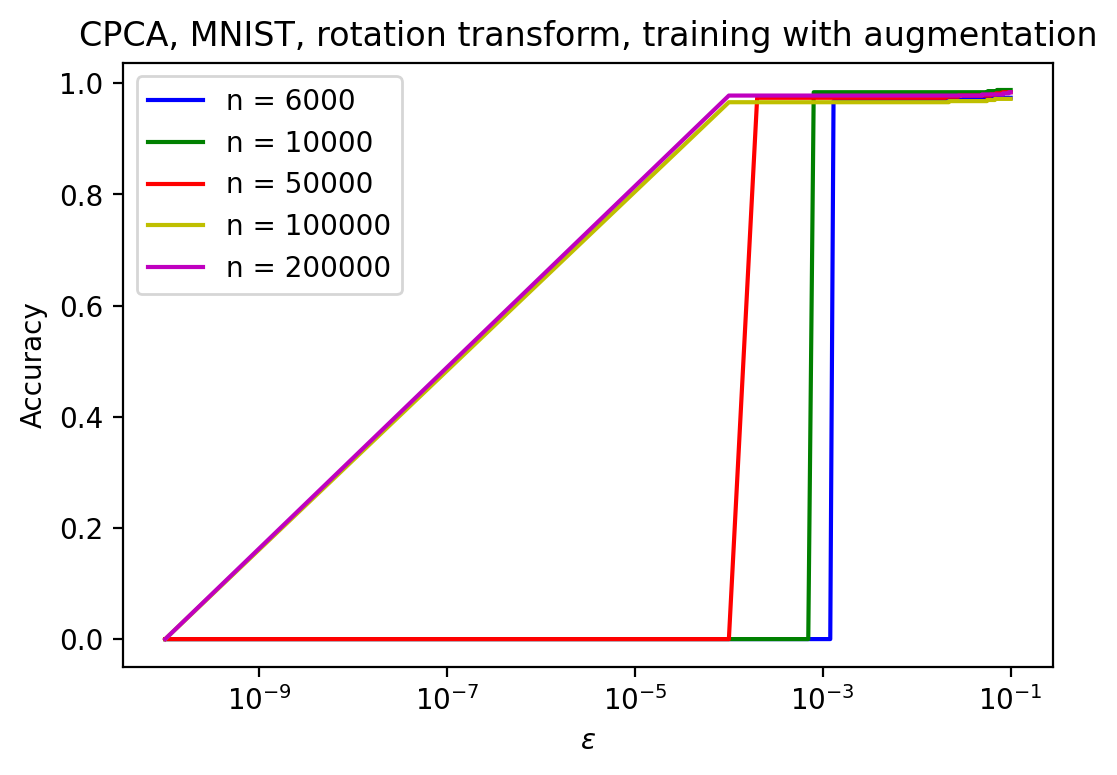
Figure 4: Clopper-Pearson certified accuracy depending on number of trials $n$ for experiment with rotation transform on MNIST.

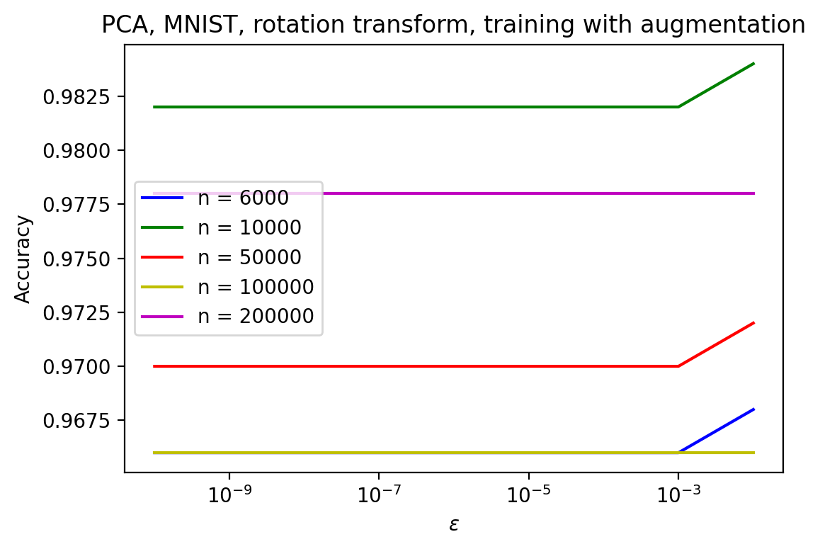
Figure 5: Probabilistically certified accuracy depending on number of samples $n$ for experiment with rotation transform on MNIST.

It can be seen that the method proposed in this paper allows to get a better bound with smaller number of samples. The reason is that we use additional information – the distribution of the random variable $Z$, unlike the CP approach which relies solely on the fact of misclassification.

Related Work

Adversarial Vulnerability. Adversarial examples (?; ?) have attracted significant attention due to vulnerability of neural networks in safety-critical scenarios. Although initially found as $\ell_{p}$-bounded attacks (?; ?), several beyond $\ell_{p}$ adversaries have been proposed that degrade performance of deep models. They include semantic perturbations, such as rotation and translation (?; ?; ?), color manipulation (?), renderer-based lightness and geometry transformation (?), parametric attribute manipulation (?), 3d scene parameters such as camera pose, sun position, global translation, rotation (?). These threats present a serious obstacle for model deployment in safety-critical real-world applications.

Certified Defenses Against Additive Perturbations. To overcome the adversarial vulnerability of deep models, several empirical defenses have been presented, however, they were found to fail against new adaptive attacks (?). This forced researchers to provide certified defenses that guarantee stable performance. A number of works have been tackling this problem for small additive perturbations from different perspectives. This includes semi-definite programming (?), interval bound propagation (?), convex relaxation (?), duality perspective (?), Satisfiability Modulo Theory (?; ?; ?). Although these methods consider small networks, randomized smoothing (?; ?; ?) and its improvements (?; ?) have been proposed as a certified defense for any network that can be applied to large-scale datasets.

Certified Defenses Against Image Transformations. Following certificates for $\ell_{p}$-bounded perturbations, several methods proposed certified robustness against semantic perturbations. Generating linear relaxation and propagating through a neural network was used in (?; ?; ?). Extensions of MCMC-based randomized smoothing (?) to the space of semantic transformations were presented in (?; ?; ?). Our work presents a probabilistic approach for certifying neural networks against different semantic perturbations. Perhaps, the closest to our approach are PROVEN (?), where authors present a framework to probabilistically certify neural networks against $\ell_{p}$ perturbations and work of (?), where authors certify a neural network in a probabilistic way by overapproximation of input regions that violate model’s robustness. However, these works do not consider probabilistic certifications under semantic transformations.

Conclusion and Future Work

We proposed a new framework CC-Cert for probabilistic certification of the robustness of DNN models to synthetic transformations and provide theoretical bounds on its robustness guarantees. Our experiments show the applicability of our approach for certification of model’s robustness to a random transformation of input. An important question that is not considered in our work is the worst-case analysis of robustness to synthetic transformations. Future work includes analysis of the discrepancy between worst-case transformations of general type and corresponding random transformations. A possible gap between certification with probability and certification in worst-case should be carefully analyzed and narrowed.

References

- [Alfarra et al. 2021] Alfarra, M.; Bibi, A.; Khan, N.; Torr, P. H.; and Ghanem, B. 2021. Deformrs: Certifying input deformations with randomized smoothing. arXiv preprint arXiv:2107.00996.
- [Anil, Lucas, and Grosse 2019] Anil, C.; Lucas, J.; and Grosse, R. 2019. Sorting out Lipschitz function approximation. In International Conference on Machine Learning, 291–301. PMLR.
- [Athalye, Carlini, and Wagner 2018] Athalye, A.; Carlini, N.; and Wagner, D. 2018. Obfuscated gradients give a false sense of security: Circumventing defenses to adversarial examples. In International conference on machine learning, 274–283. PMLR.
- [Balunović et al. 2019] Balunović, M.; Baader, M.; Singh, G.; Gehr, T.; and Vechev, M. 2019. Certifying geometric robustness of neural networks. Advances in Neural Information Processing Systems 32.
- [Boucheron, Lugosi, and Bousquet 2003] Boucheron, S.; Lugosi, G.; and Bousquet, O. 2003. Concentration inequalities. In Summer School on Machine Learning, 208–240. Springer.
- [Bunel et al. 2017] Bunel, R.; Turkaslan, I.; Torr, P. H.; Kohli, P.; and Kumar, M. P. 2017. A unified view of piecewise linear neural network verification. arXiv preprint arXiv:1711.00455.
- [Carlini and Wagner 2017a] Carlini, N., and Wagner, D. 2017a. Adversarial examples are not easily detected: Bypassing ten detection methods. In Proceedings of the 10th ACM workshop on artificial intelligence and security, 3–14.
- [Carlini and Wagner 2017b] Carlini, N., and Wagner, D. 2017b. Towards evaluating the robustness of neural networks. In 2017 ieee symposium on security and privacy (sp), 39–57. IEEE.
- [Clopper and Pearson 1934] Clopper, C. J., and Pearson, E. S. 1934. The use of confidence or fiducial limits illustrated in the case of the binomial. Biometrika 404–413.
- [Cohen, Rosenfeld, and Kolter 2019] Cohen, J.; Rosenfeld, E.; and Kolter, Z. 2019. Certified adversarial robustness via randomized smoothing. In International Conference on Machine Learning, 1310–1320. PMLR.
- [Dvijotham et al. 2018] Dvijotham, K.; Stanforth, R.; Gowal, S.; Mann, T. A.; and Kohli, P. 2018. A dual approach to scalable verification of deep networks. In UAI, volume 1, 3.
- [Ehlers 2017] Ehlers, R. 2017. Formal verification of piece-wise linear feed-forward neural networks. In International Symposium on Automated Technology for Verification and Analysis, 269–286. Springer.
- [Engstrom et al. 2018] Engstrom, L.; Tran, B.; Tsipras, D.; Schmidt, L.; and Madry, A. 2018. A rotation and a translation suffice: Fooling cnns with simple transformations.
- [Fischer, Baader, and Vechev 2020] Fischer, M.; Baader, M.; and Vechev, M. 2020. Certified defense to image transformations via randomized smoothing.
- [Goodfellow, Shlens, and Szegedy 2014] Goodfellow, I. J.; Shlens, J.; and Szegedy, C. 2014. Explaining and harnessing adversarial examples. arXiv preprint arXiv:1412.6572.
- [Gowal et al. 2018] Gowal, S.; Dvijotham, K.; Stanforth, R.; Bunel, R.; Qin, C.; Uesato, J.; Arandjelovic, R.; Mann, T.; and Kohli, P. 2018. On the effectiveness of interval bound propagation for training verifiably robust models. arXiv preprint arXiv:1810.12715.
- [Horváth et al. 2021] Horváth, M. Z.; Müller, M. N.; Fischer, M.; and Vechev, M. 2021. Boosting randomized smoothing with variance reduced classifiers.
- [Hosseini and Poovendran 2018] Hosseini, H., and Poovendran, R. 2018. Semantic adversarial examples. In Proceedings of the IEEE Conference on Computer Vision and Pattern Recognition Workshops, 1614–1619.
- [Joshi et al. 2019] Joshi, A.; Mukherjee, A.; Sarkar, S.; and Hegde, C. 2019. Semantic adversarial attacks: Parametric transformations that fool deep classifiers. In Proceedings of the IEEE/CVF International Conference on Computer Vision, 4773–4783.
- [Kanbak, Moosavi-Dezfooli, and Frossard 2018] Kanbak, C.; Moosavi-Dezfooli, S.-M.; and Frossard, P. 2018. Geometric robustness of deep networks: analysis and improvement. In Proceedings of the IEEE Conference on Computer Vision and Pattern Recognition, 4441–4449.
- [Katz et al. 2017] Katz, G.; Barrett, C.; Dill, D. L.; Julian, K.; and Kochenderfer, M. J. 2017. Reluplex: An efficient smt solver for verifying deep neural networks. In International Conference on Computer Aided Verification, 97–117. Springer.
- [Lecuyer et al. 2019] Lecuyer, M.; Atlidakis, V.; Geambasu, R.; Hsu, D.; and Jana, S. 2019. Certified robustness to adversarial examples with differential privacy. In 2019 IEEE Symposium on Security and Privacy (SP), 656–672. IEEE.
- [Levine and Feizi 2020] Levine, A., and Feizi, S. 2020. Robustness certificates for sparse adversarial attacks by randomized ablation. In Proceedings of the AAAI Conference on Artificial Intelligence, volume 34, 4585–4593.
- [Li et al. 2018a] Li, B.; Chen, C.; Wang, W.; and Carin, L. 2018a. Certified adversarial robustness with additive noise. arXiv preprint arXiv:1809.03113.
- [Li et al. 2018b] Li, T.-M.; Aittala, M.; Durand, F.; and Lehtinen, J. 2018b. Differentiable monte carlo ray tracing through edge sampling. ACM Transactions on Graphics (TOG) 37(6):1–11.
- [Li et al. 2019] Li, Q.; Haque, S.; Anil, C.; Lucas, J.; Grosse, R. B.; and Jacobsen, J.-H. 2019. Preventing gradient attenuation in Lipschitz constrained convolutional networks. Advances in Neural Information Processing Systems 32:15390–15402.
- [Li et al. 2021] Li, L.; Weber, M.; Xu, X.; Rimanic, L.; Kailkhura, B.; Xie, T.; Zhang, C.; and Li, B. 2021. TSS: Transformation-specific smoothing for robustness certification.
- [Liu et al. 2018] Liu, H.-T. D.; Tao, M.; Li, C.-L.; Nowrouzezahrai, D.; and Jacobson, A. 2018. Beyond pixel norm-balls: Parametric adversaries using an analytically differentiable renderer. arXiv preprint arXiv:1808.02651.
- [Mangal, Nori, and Orso 2019] Mangal, R.; Nori, A. V.; and Orso, A. 2019. Robustness of neural networks: A probabilistic and practical approach. In 2019 IEEE/ACM 41st International Conference on Software Engineering: New Ideas and Emerging Results (ICSE-NIER), 93–96. IEEE.
- [Mohapatra et al. 2020a] Mohapatra, J.; Ko, C.-Y.; Weng, T.-W.; Chen, P.-Y.; Liu, S.; and Daniel, L. 2020a. Higher-order certification for randomized smoothing. arXiv preprint arXiv:2010.06651.
- [Mohapatra et al. 2020b] Mohapatra, J.; Weng, T.-W.; Chen, P.-Y.; Liu, S.; and Daniel, L. 2020b. Towards verifying robustness of neural networks against a family of semantic perturbations. In Proceedings of the IEEE/CVF Conference on Computer Vision and Pattern Recognition, 244–252.
- [Moosavi-Dezfooli, Fawzi, and Frossard 2016] Moosavi-Dezfooli, S.-M.; Fawzi, A.; and Frossard, P. 2016. Deepfool: a simple and accurate method to fool deep neural networks. In Proceedings of the IEEE Conference on Computer Vision and Pattern Recognition, 2574–2582.
- [Paley and Zygmund 1930] Paley, R., and Zygmund, A. 1930. On some series of functions,(1). In Mathematical Proceedings of the Cambridge Philosophical Society, volume 26, 337–357. Cambridge University Press.
- [Paszke et al. 2019] Paszke, A.; Gross, S.; Massa, F.; Lerer, A.; Bradbury, J.; Chanan, G.; Killeen, T.; Lin, Z.; Gimelshein, N.; Antiga, L.; et al. 2019. Pytorch: An imperative style, high-performance deep learning library. Advances in Neural Information Processing Systems 32:8026–8037.
- [Raghunathan, Steinhardt, and Liang 2018] Raghunathan, A.; Steinhardt, J.; and Liang, P. 2018. Semidefinite relaxations for certifying robustness to adversarial examples. arXiv preprint arXiv:1811.01057.
- [Riba et al. 2020] Riba, E.; Mishkin, D.; Ponsa, D.; Rublee, E.; and Bradski, G. 2020. Kornia: an open source differentiable computer vision library for pytorch. In Proceedings of the IEEE/CVF Winter Conference on Applications of Computer Vision, 3674–3683.
- [Salman et al. 2019] Salman, H.; Yang, G.; Li, J.; Zhang, P.; Zhang, H.; Razenshteyn, I.; and Bubeck, S. 2019. Provably robust deep learning via adversarially trained smoothed classifiers. arXiv preprint arXiv:1906.04584.
- [Serrurier et al. 2021] Serrurier, M.; Mamalet, F.; González-Sanz, A.; Boissin, T.; Loubes, J.-M.; and del Barrio, E. 2021. Achieving robustness in classification using optimal transport with hinge regularization. In Proceedings of the IEEE/CVF Conference on Computer Vision and Pattern Recognition, 505–514.
- [Singh et al. 2019] Singh, G.; Gehr, T.; Püschel, M.; and Vechev, M. 2019. An abstract domain for certifying neural networks. Proceedings of the ACM on Programming Languages 3(POPL):1–30.
- [Szegedy et al. 2013] Szegedy, C.; Zaremba, W.; Sutskever, I.; Bruna, J.; Erhan, D.; Goodfellow, I.; and Fergus, R. 2013. Intriguing properties of neural networks. arXiv preprint arXiv:1312.6199.
- [Tramer et al. 2020] Tramer, F.; Carlini, N.; Brendel, W.; and Madry, A. 2020. On adaptive attacks to adversarial example defenses. arXiv preprint arXiv:2002.08347.
- [Weng et al. 2019] Weng, L.; Chen, P.-Y.; Nguyen, L.; Squillante, M.; Boopathy, A.; Oseledets, I.; and Daniel, L. 2019. PROVEN: Verifying robustness of neural networks with a probabilistic approach. In International Conference on Machine Learning, 6727–6736. PMLR.
- [Wong and Kolter 2018] Wong, E., and Kolter, Z. 2018. Provable defenses against adversarial examples via the convex outer adversarial polytope. In International Conference on Machine Learning, 5286–5295. PMLR.
- [Xiao et al. 2018] Xiao, C.; Zhu, J.-Y.; Li, B.; He, W.; Liu, M.; and Song, D. 2018. Spatially transformed adversarial examples. arXiv preprint arXiv:1801.02612.
- [Zhai et al. 2020] Zhai, R.; Dan, C.; He, D.; Zhang, H.; Gong, B.; Ravikumar, P.; Hsieh, C.-J.; and Wang, L. 2020. Macer: Attack-free and scalable robust training via maximizing certified radius. arXiv preprint arXiv:2001.02378.