Efficient Computation of Periodic Orbits of Forced Rayleigh Equation in the Framework of Novel Asymptotic Structures

Abstract

Higher precision efficient computation of period 1 relaxation oscillations of strongly nonlinear and singularly perturbed Rayleigh equations with external periodic forcing is presented. The computations are performed in the context of conventional renormalization group method (RGM). We demonstrate that although a slight homotopically modified RGM could generate approximate periodic orbits that agree qualitatively with the exact orbits, the method, nevertheless, fails miserably to reduce the large quantitative disagreement between the theoretically computed results with that of exact numerical orbits. In the second part of the work we present a novel asymptotic analysis incorporating SL(2,R) invariant nonlinear deformation of slower time scales, $t_{n}=\varepsilon^{n}t,\ n\rightarrow\infty,\ \varepsilon<1$, for asymptotic late time $t$, to a nonlinear time $T_{n}=t_{n}\sigma(t_{n})$, where the deformation factor $\sigma(t_{n})>0$ respects some well defined SL(2,R) constraints. Motivations and detailed applications of such nonlinear asymptotic structures are explained in performing very high accuracy ($>98\%$) computations of relaxation orbits. Existence of an interesting condensation and rarefaction phenomenon in connection with dynamically adjustable scales in the context of a slow-fast dynamical system is explained and verified numerically.

Keywords: Asymptotic Analysis, Nonlinear Ordinary Differential Equations, Renormalization Group

Mathematics Subject Classification: 34E10, 34A34, 34E15

1 Introduction

The aim of the present paper is to formulate an efficient computation scheme of periodic orbits of a strongly nonlinear oscillator [1, 2, 3, 4]. The importance of high precision computation in applied mathematics and science need not be overemphasized [5]. The higher precision quantitatively accurate computation of periodic orbits is facilitated in the framework of a novel asymptotic analysis [6, 7, 8, 9], so as to allow significant numerical improvements in the computations of periodic orbits by the conventional asymptotic techniques such as renormalization group method(RGM) [10], multiple scale method (MSM) [1], homotopy analysis method [11, 12] etc. As a prototype of strongly nonlinear oscillator, we consider here singularly perturbed Rayleigh Equation (SRLE) [1, 4] equation with an external periodic excitation

$$\varepsilon\ddot{x}+\left(\frac{1}{3}\dot{x}^{3}-\dot{x}\right)+x=\varepsilon\ F\cos\left(\Omega\ t\right),$$ (1.1)

where dots are used to designate the derivatives with respect to time. Rayleigh Equation, either regular or singularly perturbed, and a close cousin of Van der Pol equation [7], is one of the extensively studied nonlinear oscillatory systems because of its wide applications in acoustics, physiology and cardiac cycles, solid mechanics, electronics and nonlinear electrical circuits, musical instruments and many other different fields [1, 2, 13, 14]. Singularly perturbed Rayleigh equation is equivalently related closely to the regularly perturbed Rayleigh equation (RLE)

$$\ddot{x}+\varepsilon\left(\frac{1}{3}\dot{x}^{3}-\dot{x}\right)+x=\varepsilon\ F\cos\left(\Omega\ t\right),$$ (1.2)

for a large nonlinearity parameter $\varepsilon>1$. It is well known that both the Rayleigh equations $\left(\text{\ref{SFRL Eqn}}\right)$ and $\left(\text{\ref{RFRL Eqn}}\right)$ with $F=0$ have unique, stable periodic solutions (orbits), known as the limit cycle in the appropriate phase plane for all $\varepsilon>0$. However, the periodic orbit for singularly perturbed equation and hence, for larger values of $\varepsilon\gtrapprox 1$ in the regular Rayleigh equation, the periodic cycle is a relaxation oscillation, consisting of slow and fast developing components. Existence of slow and fast motions makes traditional analytical techniques ineffective in an efficient estimation of such relaxation oscillations [15, 16]. Dynamical systems experiencing the fast-slow motions appear widely in engineering and other applied sciences [12]. The slow-fast periodic motions in such dynamical systems cannot be easily tackled, because such slow-fast periodic motions need many more harmonic terms to get appropriate approximate solutions. Usually, the fast movement behaves like an impulsive motion and so grows very quickly, where as the slow movement is like almost zero velocity movement and hence the system relaxes very slowly. As will become evident, the present approach equipped with novel asymptotic quantities, however, would yield such high precision orbits with much smaller number of harmonic terms only.

To recall, the general study, particularly in the context of high precision computations, of orbits of the nonlinear ordinary differential equations (NODE) has always been a challenging task. Exact computation/determination of analytic solutions of such differential equations is not always possible because most of them are not generally reducible into exactly integrable form involving standard functions [3, 2]. Moreover, a wide class of NODEs are known to have sensitive dependence on initial conditions, leading to late time asymptotic unpredictability and chaotic behaviour. The transition from small time continuity on initial conditions to the final late time loss of continuity in a nonlinear system generally proceeds via a universal route, called the period doubling bifurcation route to chaos. As one or more control (nonlinearity) parameter(s) $\varepsilon$ (say) in the nonlinear system is slowly changed from smaller values to larger values progressively, the system experiences a sequence of bifurcations in which a period $n$ orbit is changed suddenly to a period $2n$ orbit at the bifurcation point $\varepsilon_{n}$ leading finally to chaos [3, 2, 17] . In the absence of exact computability (except for very special cases, for instance, the Duffing oscillator) of amplitudes, phases and solutions of isolated periodic orbits (Limit Cycles), along with precise enumeration of period doubling routes of nonlinear systems, higher precision asymptotic determinations of the periodic $2n$ cycles are interesting, not only on theoretical ground but also have significant applications[12].

Over past few decades, various non-perturbative modifications of naive perturbation method such as Method of Multiple Scales, Method of Boundary Layer [2], WKB Method [4], Homotopy Averaging Method [18], Homotopy Analysis Method [11], Variational Iteration Method [19], homotopy RG method[20] etc., have been investigated and advocated widely for faster and efficient computation of periodic oscillations of strongly nonlinear systems as well as to singularly perturbed problems, that should yield reasonable fits with experimental values for any value of the control parameter $\varepsilon>0$. But over time it has become evident that none of the these asymptotic methods could yield uniformly valid approximate solutions to the system variables concerned, both for a large control parameter space as well as for sufficiently large time [16], unless special care and methods are invented and considered. Recently, Xu and Luo [15] presented semi-analytic implicit mapping scheme for relaxation oscillations of forced Van der Pol oscillator. The semi-analytic method is also applied in various other nonlinear systems such as double pendulum, and many others, see for instance, [21]. In [22], Luo presented higher precision computations of periodic orbits in the context of so called generalized averaging method. An efficient computation of periodic orbits of forced Van der Pol-Duffing equation was also presented recently [12] in the context of homotopy analysis method. In all these cited works a large number of harmonic terms, however, are necessary for the said higher precision computations of periodic orbits. Need for invoking extensive numerical analysis in attaining highly accurate periodic orbits, as evidenced in [22, 15, 12], based on different asymptotic modeling and methods, make rooms for further research in this interesting area of NODE looking for new and novel theoretical insights that would not only reduce the burden of numerical analysis and computational time, but might also offer new insights into asymptotic properties of nonlinear dynamics.

In the present work, we investigate a modified and improved renormalization group (RG) method (IRGM) incorporating a novel asymptotic structure, called $SL(2,\mathbb{R})$ duality structure, that is introduced and is being investigated previously by Datta et. al. [6, 7, 8, 9, 23] in various nonlinear applications. An application of IRGM and duality structure was presented in [7] in the context of Rayleigh equation $\left(\text{\ref{RFRL Eqn}}\right)$ and Van der Pol equation (without forcing)

$$\ddot{x}+\varepsilon\ \dot{x}\left(x^{2}-1\right)+x=0,$$ (1.3)

where relative advantage of IRGM over Homotopy analysis method was established along with high precession analysis of limit cycle orbits (see also [20]). By efficiency of an asymptotic method we mean that one could yield $95\%$ or above fits with the experimental values, only with a lower order approximate computation (1st or 2nd order, in the perturbative sense), while the other theory would require very high order of computations to attain that amount of precision (see for instance, [22, 12]). We now apply IRGM equipped with novel renormalized asymptotic duality structures in obtaining high precision fits with the theoretical results and that of the experimental results for periodic orbits of periodically forced Rayleigh oscillators. To emphasize once more, continual improvements in asymptotic techniques is indeed a very important research area in applied mathematics, not only for a better theoretical understanding of periodic or nonperiodic orbits of nonlinear oscillator problems, but must also have significant engineering and other applications [12, 15, 21]. A substantial extension of the $SL(2,\mathbb{R})$ asymptotic analysis is also formulated recently [24].

To recall, the improvement of RG Method was made possible in [7] by introduction of $SL(2,\mathbb{R})$ invariant, renormalized (control) variables, which can be used to ensure an improved convergence of approximate solutions through continuous deformations to the exact solution of the nonlinear oscillation problem concerned, with any desired accuracy level. The introduction of continuous deformation is based on the novel idea of nonlinear time [6, 8, 9, 24], incorporating ideas of asymptotic duality structure and dynamically adjustable time scales [8, 9, 24]. It is well known that $\left(\text{\ref{RFRL Eqn}}\right)$ has unique limit cycle solution for $\varepsilon>0$ under the action of near resonant small external periodic force, i.e. when $F\neq 0$ and the frequency $\Omega$ of the external applied force is close to the frequency of the system or $\Omega\approx 1$. In this article we shall find, for a given $\varepsilon>1$, the values of $F$ and $\Omega$ for which a significant quantitative difference can be observed between the exactly computed numerical limit cycle solution and that computed from RGM. Next we shall improve the initial RG approximation of the exact solution, using the improved RGM and dynamical time scales along independent phase space variables, achieving better and faster convergence to the exact solution. In fact, this article is an extension of the work in [7] for the forced Rayleigh equations with strong nonlinearity, and hence singularly perturbed, equations $\left(\text{\ref{SFRL Eqn}}\right)$ and $\left(\text{\ref{RFRL Eqn}}\right)$. Further, the numerical results presented here demonstrate an interesting condensation and rarefaction phenomenon in the numerically computed data points based on the improved RGM calculations and involving the dynamically adjustable time scales (c.f. Section 4) thus verifying explicitly the dynamics of slow fast behaviours. Judicious choices of dynamical time scales would also help reducing the computational complexity in achieving high precision results.

The paper is organized as follows. In Section 2, we review RG method in the context of singular Rayleigh equation. The failure of usual RG method is next presented in subsection 2.1 when the singularly perturbed problem is presented as slow-fast system in the phase plane. In subsection 2.2, we demonstrate that the RG method could be made effective when the singular problem is translated into a regular problem with a large nonlinearity parameter but, nevertheless, interpreted in the sense of homotopy deformation [20] involving a small homotopy parameter $\mu$. The desired result, viz., the limit cycle solution, is then obtained by continuity by fixing finally $\mu$ to the limiting value $\mu=1$. In the next two subsections 2.3 and 2.4, we present analogous computations of homotopy aided RG amplitude and phase equations of regular Rayleigh equation with strong nonlinearity, and singular Rayleigh equation with various alternate choices of homotopy deformations respectively. Interestingly, we point out that final frequency-amplitude equations for all these various homotopy choices are identical at the order $O(1)$ and hence independent of how the homotopy perturbation schemes are invoked and implemented. In Section 3, we present the analysis based on the novel asymptotic structures and show in Section 4, how the said structures could successfully yield highly efficient fits with the phase plane orbits of relaxation oscillations that could have been attained in the traditional schemes only with very high order of asymptotic computations involving many more harmonic terms. In the discussion subsection 4.1, we compare our results with those available in current literature. Finally, we summarize our main conclusions, and remark on future scope of research in the concluding Section 5.

2 Renormalization Group Method and Singular Rayleigh Equation

The Renormalization Group Method (RGM) has a very hallowed history, being originally formulated in the context of quantum field theory and critical phenomena [10] and later had seen a wide range of applications in various nonlinear problems, such as solid state physics, fluid mechanics, cosmology, fractal geometry and many others. The theory of renormalization group is known to be closely related to the concept of intermediate asymptotics [25]. The applications of RGM to the NODE was first considered by Chen, Goldenfeld and Oono (CGO) in [26]. Different authors [27, 7, 28] used the RGM in the computations of analytic approximations of solutions of various nonlinear differential systems.

Studies by different authors [26, 28] reveal that the RGM has various practical advantages over other conventional methods such as Boundary Layer theory, method of Multiple Scales, WKB method etc. In traditional methods, various guage functions, such as fractional power laws or exponential or logarithmic functions of nonlinearity parameters such as $\varepsilon$ are usually introduced in an ad hoc manner. However, such gauge functions arise quite naturally from the algorithm of RGM. One does not require to fix such a gauge function from asymptotic matching, or power counting. However, RGM does have its own limitations. It is shown in [7] that RGM fails to give uniformly valid approximate solutions for larger values of $\varepsilon\gtrapprox O(1)$. Liu [20] presented a detailed analysis of failures of RGM and formulated an improvement of RGM by the so-called Homotopy Renormalization method (see also [29]). In Section 2.1, we show that the perturbative RGM also fails to yield physically relevant results in the singular Rayleigh system.

The limit cycle solution of the system $\left(\text{\ref{RFRL Eqn}}\right)$ with $F=0$ is studied by Palit and Datta in [7] for different values of $\varepsilon>0$. The authors observed that the higher order computations of this system using RGM fail to improve the classical results. Further, there does not seem to exist any handle in RGM to ensure convergence of the approximate solutions to the exact (numerical) solution to within any specified error bound. Moreover, vary laborious computations needed generally in the classical RGM for higher order calculations make it quite improbable for higher order computations. Thus, an improvement of this method is necessary so that one can ensure convergence of the approximate solutions to the exact one through a minimal level of computation. With this aim, the theory of RGM is improved by introduction of some homotopy like deformation parameters, in association with the framework of an asymptotically nonlinear time, which we shall discuss in the next section. These control (deformation) parameters essentially ensured the convergence, using the idea of continuous deformation of the topological homotopy deformation theory. The introduction of these control parameters induces the convergence to the approximate solutions with only a minimal order computation, reducing the computational complexity of RGM and at the same time improves its efficacy.

The formalism of RGM for the differential equation was introduced by CGO [26]. This method starts with the naive perturbative solution of an initial value problem having initial time $t_{0}$. For periodic oscillations, it involves terms like

$$\left(t-t_{0}\right)\sin t\text{, }\left(t-t_{0}\right)\cos t\text{ etc.}$$

which are secular or unbounded as $t$ increases asymptotically. Consequently the resultant perturbative solution fails to remain periodic and breaks down for sufficiently large $t$. In order to eliminate this kind of secular terms CGO introduced an arbitrary time $\tau$ and split the time difference $t-t_{0}$ as $t-\tau+\tau-t_{0}$ and used RGM to generate a periodic solution out of this naive perturbative series. One important step, which will be referred to again later in this section, is the fact that the solution $x$ should not depend on the arbitrary time $\tau$. Therefore, $x$ must be independent of $\tau$ so that one obtains the renormalization condition

$$\left.\frac{dx}{d\tau}\right|_{\tau=t}=0\text{.}$$ (2.1)

DeVille [27] introduced an equivalent simplified version of the RGM which was adopted by Palit and Datta [7]. We shall investigate the solution of the of the systems $\left(\text{\ref{SFRL Eqn}}\right)$ and $\left(\text{\ref{RFRL Eqn}}\right)$ using the approach given by DeVille. In this method the naive perturbative solution of an initial value nonlinear differential system is derived in terms of complex numbers involving a complex constant of motion $A$ $($see for detail section 5 in [27]$)$. The initial time $t_{0}$ is taken as arbitrary with the initial condition $w\left(t_{0}\right)$. In the second step they renormalize the initial condition into $w\left(t_{0}\right)$ by absorbing the time independent and bounded terms in the naive expansion. This step renormalizes the constant of motion $A$ and generates its counterpart $\mathcal{A=A}\left(t_{0}\right)$ by absorbing the homogeneous parts of the solution into it. This leaves the solution $x$ having few secular terms involving

$$\left(t-t_{0}\right)e^{i\left(t-t_{0}\right)},\ \left(t-t_{0}\right)^{2}e^{i\left(t-t_{0}\right)}\text{ etc.}$$

along with their complex conjugates. In the third step the renormalization condition $\left(\text{\ref{CGO-RG Eq}}\right)$ becomes

$$\left.\frac{dx}{dt_{0}}\right|_{t_{0}=t}=0$$ (2.2)

which under the transformation

$$\mathcal{A=}\frac{R}{2}e^{i\theta}$$ (2.3)

generates RG flow equations in the amplitude $R$ and the phase $\theta$. To derive frequency response curve of a forced oscillator, one would generally require to replace $\theta$ by $\theta(t)=\Omega t+\phi(t)$, that eliminates the zeroth order constant term, in favour of a term involving the detuning parameter $\sigma$, in the right hand side of the phase flow equation. Here, $\Omega=\omega+\sigma\varepsilon$, is the response frequency determined by the natural frequency $\omega$ and $O(\varepsilon)$ detuning $\sigma$ (c.f. Section 2.2-4 and Appendix). A brief review of RGM in the context of forced Rayleigh equation near primary resonance, along with the associated frequency-amplitude response equation and the associated stability analysis [1] is given in Appendix.

2.1 Failure of RGM in Slow-fast system

To present the case of failure of the classical RGM in the Rayleigh slow-fast system, we consider, for simplicity, the singular Rayleigh equation $\left(\text{\ref{SFRL Eqn}}\right)$ with $F=0$ and $0<\varepsilon<1\$ which on differentiating with respect to time has the form

$$\varepsilon\dddot{x}+\left(\dot{x}^{2}-1\right)\ddot{x}+\dot{x}=0.$$

Assuming

$$\dot{x}=y$$

one gets

$$\varepsilon\ddot{y}+\left(y^{2}-1\right)\dot{y}+y=0,\ 0<\varepsilon<1.$$ (2.4)

This is nothing but the singular Van der Pol equation. Since the limit cycle solution of $\left(\text{\ref{Singular VdP Eq}}\right)$ does not depend upon the initial condition, so without loss of generality, we take the initial condition as

$$y\left(t_{0}\right)=A_{0}\text{ and }\dot{y}\left(t_{0}\right)=B_{0}\text{.}$$ (2.5)

We write equation (2.4) as an autonomous system

$$\dot{y} =z$$ (2.6a)

$$\varepsilon\dot{z} =-\left(y^{2}-1\right)z-y$$ (2.6b)

and the initial condition $$\left(\text{\ref{SVdP IC}}\right)$$ can be written as

$$y\left(t_{0}\right)=A_{0}\text{ and }z\left(t_{0}\right)=B_{0}\text{.}$$ (2.7)

We introduce the standard boundary layer scaling time $\tau$ using the transformation

$$t=\varepsilon\ \tau$$ (2.8)

and hence rewrite the autonomous system $\left(\text{\ref{SVdP Eq}}\right)$ as

$$y^{\prime} =\varepsilon z$$ (2.9a)

$$z^{\prime} =-\left(y^{2}-1\right)z-y$$ (2.9b)

with the initial conditions $$y\left(\tau_{0}\right)=A_{0}\text{\ and \ }z\left(\tau_{0}\right)=B_{0}\text{,} \tau \tau_{0}=\frac{t_{0}}{\varepsilon}\text{.}$$ where ^′ represents the derivative with respect to the variable and

Taking

$$y\left(\tau\right) =y_{0}\left(\tau\right)+\varepsilon\ y_{1}\left(\tau\right)+\varepsilon^{2}y_{2}\left(\tau\right)+\cdots$$ (2.10a)

$$\text{and }z\left(\tau\right) =z_{0}\left(\tau\right)+\varepsilon\ z_{1}\left(\tau\right)+\varepsilon^{2}z_{2}\left(\tau\right)+\cdots$$ (2.10b)

from $$\left(\text{\ref{SVdP New}}\right)$$ we get different order relations as

zero-th order $$:y_{0}^{\prime}\left(\tau\right)=0\qquad\text{with }y_{0}\left(\tau_{0}\right)=A_{0},$$ (2.11a)

$$\varepsilon\text{ order} :y_{1}^{\prime}\left(\tau\right)=z_{0}\left(\tau\right)\qquad\text{with }y_{1}\left(\tau_{0}\right)=0,$$ (2.11b)

$$\varepsilon^{2}\text{ order} :y_{2}^{\prime}\left(\tau\right)=z_{1}\left(\tau\right)\qquad\text{with }y_{2}\left(\tau_{0}\right)=0,$$ (2.11c)

$$\cdots\quad\cdots\quad\cdots\quad\cdots\quad\cdots\quad\cdots$$

and

zero-th order $$:z_{0}^{\prime}+z_{0}\left(y_{0}^{2}-1\right)=-y_{0}\qquad\text{with }z_{0}\left(\tau_{0}\right)=B_{0},$$ (2.12a)

$$\varepsilon\text{ order} :z_{1}^{\prime}+z_{1}\left(y_{0}^{2}-1\right)=-y_{1}-2y_{0}y_{1}z_{0}\qquad\text{with }z_{1}\left(\tau_{0}\right)=0,$$ (2.12b)

$$\varepsilon^{2}\text{ order} :z_{2}^{\prime}+z_{2}\left(y_{0}^{2}-1\right)=-y_{2}-z_{0}\left(y_{1}^{2}+2y_{0}y_{2}\right)-2y_{0}y_{1}z_{1}\qquad\text{with }z_{2}\left(\tau_{0}\right)=0.$$ (2.12c)

$$\cdots\quad\cdots\quad\cdots\quad\cdots\quad\cdots\quad\cdots$$

The naive perturbative solutions of $$\left(\text{\ref{SVdP Pert Eqy}}\right) \left(\text{\ref{SVdP Pert Eqz}}\right) \varepsilon$$ and upto order are

$$y_{0}\left(\tau\right) =A_{0},$$

$$y_{1}\left(\tau\right) =-\frac{1}{\left(A_{0}^{2}-1\right)}\left(B_{0}+\frac{A_{0}}{A_{0}^{2}-1}\right)e^{-\left(A_{0}^{2}-1\right)\left(\tau-\tau_{0}\right)}-\frac{A_{0}}{A_{0}^{2}-1}\left(\tau-\tau_{0}\right)+\frac{1}{\left(A_{0}^{2}-1\right)}\left(B_{0}+\frac{A_{0}}{A_{0}^{2}-1}\right)$$

and

$$z_{0}\left(\tau\right)=\left(B_{0}+\frac{A_{0}}{A_{0}^{2}-1}\right)e^{-\left(A_{0}^{2}-1\right)\left(\tau-\tau_{0}\right)}-\frac{A_{0}}{A_{0}^{2}-1},$$

$$z_{1}\left(\tau\right) =\dfrac{2A_{0}}{\left(A_{0}^{2}-1\right)^{2}}\left(B_{0}+\dfrac{A_{0}}{A_{0}^{2}-1}\right)^{2}e^{-\left(A_{0}^{2}-1\right)\left(\tau-\tau_{0}\right)}+\frac{A_{0}}{\left(A_{0}^{2}-1\right)^{3}}\left(1+\frac{2A_{0}^{2}}{\left(A_{0}^{2}-1\right)}\right)e^{-\left(A_{0}^{2}-1\right)\left(\tau-\tau_{0}\right)}$$

$$+\left(1+\frac{2A_{0}^{2}}{\left(A_{0}^{2}-1\right)}\right)\frac{1}{\left(A_{0}^{2}-1\right)^{2}}\left(B_{0}+\frac{A_{0}}{A_{0}^{2}-1}\right)e^{-\left(A_{0}^{2}-1\right)\left(\tau-\tau_{0}\right)}-\dfrac{2A_{0}}{\left(A_{0}^{2}-1\right)^{2}}\left(B_{0}+\dfrac{A_{0}}{A_{0}^{2}-1}\right)^{2}e^{-2\left(A_{0}^{2}-1\right)\left(\tau-\tau_{0}\right)}$$

$$+\left(1-2A_{0}B_{0}\right)\frac{1}{\left(A_{0}^{2}-1\right)}\left(B_{0}+\frac{A_{0}}{A_{0}^{2}-1}\right)e^{-\left(A_{0}^{2}-1\right)\left(\tau-\tau_{0}\right)}\left(\tau-\tau_{0}\right)+\frac{A_{0}}{\left(A_{0}^{2}-1\right)^{2}}\left(1+\frac{2A_{0}^{2}}{\left(A_{0}^{2}-1\right)}\right)\left(\tau-\tau_{0}\right)$$

$$+\dfrac{A_{0}^{2}}{A_{0}^{2}-1}\left(B_{0}+\dfrac{A_{0}}{A_{0}^{2}-1}\right)e^{-\left(A_{0}^{2}-1\right)\left(\tau-\tau_{0}\right)}\left(\tau-\tau_{0}\right)^{2}$$

$$-\frac{1}{\left(A_{0}^{2}-1\right)^{2}}\left(1+\frac{2A_{0}^{2}}{\left(A_{0}^{2}-1\right)}\right)\left(B_{0}+\frac{2A_{0}}{A_{0}^{2}-1}\right)\text{.}$$

We apply classical RGM (See Appendix) by introducing an arbitrary intermediate time $\lambda$ to split the time interval $\left(\tau-\tau_{0}\right)$ as $\left(\tau-\lambda\right)+\left(\lambda-\tau_{0}\right)$ and take

$$A_{0} =Z_{1}\mathcal{A}\left(\lambda\right)$$

$$\text{and }B_{0} =Z_{2}\mathcal{B}\left(\lambda\right)$$

where

$$Z_{1} =\sum_{n=0}^{\infty}a_{n}\left(\tau_{0},\lambda\right)\varepsilon^{n}=a_{0}+a_{1}\varepsilon+a_{2}\varepsilon^{2}+...$$

$$\text{and }Z_{2} =\sum_{n=0}^{\infty}b_{n}\left(\tau_{0},\lambda\right)\varepsilon^{n}=b_{0}+b_{1}\varepsilon+b_{2}\varepsilon^{2}+...$$

with

$$a_{0}=1,\ b_{0}=1$$

so that

$$A_{0} =\mathcal{A}\left(1+a_{1}\varepsilon+...\right),$$

$$B_{0} =\mathcal{B}\left(1+b_{1}\varepsilon+...\right).$$

The divergent secular terms involving $\left(\lambda-\tau_{0}\right)$ are absorbed in different orders giving the values of $a_{1}$ and $b_{1}$ etc. We finally obtain the flow equations

$$\frac{d\mathcal{A}}{d\tau}=\varepsilon\left[-\frac{\mathcal{A}}{\left(\mathcal{A}^{2}-1\right)}-\frac{d\mathcal{B}}{d\tau}\frac{1}{\left(\mathcal{A}^{2}-1\right)}+\frac{2\mathcal{AB}}{\left(\mathcal{A}^{2}-1\right)^{2}}\frac{d\mathcal{A}}{d\tau}-\frac{d}{d\tau}\left(\frac{\mathcal{A}}{\left(\mathcal{A}^{2}-1\right)^{2}}\right)\right]+O\left(\varepsilon^{2}\right)$$

and

$$\frac{d\mathcal{B}}{d\tau}=\frac{d}{d\tau}\left(\frac{\mathcal{A}}{\left(\mathcal{A}^{2}-1\right)}\right)+\varepsilon\frac{\mathcal{A}}{\left(\mathcal{A}^{2}-1\right)^{2}}\left(1+2\frac{\mathcal{A}^{2}}{\mathcal{A}^{2}-1}\right)+\varepsilon\frac{d}{d\tau}\left(\frac{1}{\left(\mathcal{A}^{2}-1\right)^{2}}\left(1+2\frac{\mathcal{A}^{2}}{\mathcal{A}^{2}-1}\right)\left(\mathcal{B}+2\frac{\mathcal{A}}{\mathcal{A}^{2}-1}\right)\right)+O\left(\varepsilon^{2}\right)$$

which in terms of the variable $t$ become

$$\frac{d\mathcal{A}}{dt}=-\frac{\mathcal{A}}{\left(\mathcal{A}^{2}-1\right)}+O\left(\varepsilon\right)$$

and

$$\frac{d\mathcal{B}}{dt}=\frac{d}{dt}\left(\frac{\mathcal{A}}{\left(\mathcal{A}^{2}-1\right)}\right)+\frac{\mathcal{A}}{\left(\mathcal{A}^{2}-1\right)^{2}}\left(1+2\frac{\mathcal{A}^{2}}{\mathcal{A}^{2}-1}\right)+O\left(\varepsilon\right)$$

respectively. For steady state (c.f. Appendix) we must have $\frac{d\mathcal{A}}{dt}=0$ and $\frac{d\mathcal{B}}{dt}=0$ which give $\mathcal{A}=0$ and $\mathcal{B}=0$. So, the classical RGM fails to give any limit cycle solution for the singular Van der Pol equation $\left(\text{\ref{Singular VdP Eq}}\right)$ [20]. The failure could also be verified for the forced singular problem with some extra computations. However, we note, in retrospect, that RGM, extended in the context of a homotopy deformation, is strong enough to restore the desired periodic cycles when the singular problem is transformed into a regular perturbation problem with a large value of the nonlinearity parameter $\bar{\varepsilon}>1$. We demonstrate this fact in following three subsections for various choices of homotopy deformations for the original singular problem.

2.2 Homotopy and RGM: Case 1: SRLE

In Appendix, we detail out briefly the formal RGM computations of amplitude and phase flow equations for a general periodically forced Rayleigh equation for any $\varepsilon>0$. Here we consider the singular Rayleigh equation $\left(\text{\ref{SFRL Eqn}}\right)$ with $\varepsilon<1$. It can be written as

$$\ddot{x}+\omega^{2}\left(\frac{1}{3}\dot{x}^{3}-\dot{x}\right)+\omega^{2}x=F\cos\left(\Omega t\right)$$ (2.13)

where,

$$\omega=\sqrt{\frac{1}{\varepsilon}}>1\text{.}$$

As noted already, RGM is a powerful asymptotic method that aims to improve upon the limitations of naive perturbation expansions of periodic responses in a nonlinear system. It is therefore imperative that the nonlinearity in the system is weak and the associated non-linearity parameter $\varepsilon$ is small. In order to study its limit cycle solution we consider homotopically deformed equation

$$\ddot{x}+\omega^{2}\mu\left(\frac{1}{3}\dot{x}^{3}-\dot{x}\right)+\omega^{2}x=F\mu\cos\left(\Omega t\right)\text{ for }\mu\leq 1,$$ (2.14)

which becomes the Rayleigh equation $\left(\text{\ref{SRLE New}}\right)$ for $\mu=1$. Taking

$$\Omega=\omega+\mu\sigma$$ (2.15)

and

$$x\left(t\right)=x_{0}\left(t\right)+\mu\ x_{1}\left(t\right)+\mu^{2}x_{2}\left(t\right)+\cdots$$ (2.16)

and following the steps of Appendix, we get the RG flow equations as

$$\dfrac{dR}{dt}=\mu\left(\dfrac{R}{2}-\dfrac{R^{3}}{8}\omega^{2}\right)\omega^{2}-\dfrac{F}{2\omega}\ \mu\sin\theta+O\left(\mu^{2}\right)$$ (2.17)

and

$$\dfrac{d\theta}{dt}=\omega-\dfrac{F}{2R\omega}\mu\cos\theta+O\left(\mu^{2}\right)\text{.}$$ (2.18)

The renormalized solution after taking the limit $t\rightarrow\infty$ and eliminating the secular terms is

$$x\left(t\right)=R\left(t\right)\cos\left(\theta\left(t\right)\right)+\frac{1}{96}\mu\omega^{3}R^{3}\left(t\right)\sin\left(3\theta\left(t\right)\right)$$ (2.19)

where, $R\left(t\right)$ and $\theta\left(t\right)$ are obtained from the solution of the RG flow equations. Invoking continuity of deformed system and letting $\mu\rightarrow 1^{-}$ in $\left(\text{\ref{SRLE RG Eq1}}\right)$, $\left(\text{\ref{SRLE RG Eq2}}\right)$ and $\left(\text{\ref{SRLE RG Sol}}\right)$ we get,

$$\dfrac{dR}{dt} =\left(\dfrac{R}{2}-\dfrac{R^{3}}{8}\omega^{2}\right)\omega^{2}-\dfrac{F}{2\omega}\sin\theta$$ (2.20)

$$\dfrac{d\theta}{dt} =\omega-\dfrac{F}{2R\omega}\cos\theta$$ (2.21)

and

$$x\left(t\right)=R\left(t\right)\cos\left(\theta\left(t\right)\right)+\frac{1}{96}\omega^{3}R^{3}\left(t\right)\sin\left(3\theta\left(t\right)\right).$$ (2.22)

As, by continuity, $\mu$ attains the limiting value $\mu=1$, one gets by writing

$$\theta=\phi+\Omega\ t=\phi+\left(\omega+\sigma\right)t$$ (2.23)

the flow equations as,

$$\dfrac{dR}{dt}=\left(\dfrac{R}{2}-\dfrac{R^{3}}{8}\omega^{2}\right)\omega^{2}-\dfrac{F}{2\omega}\sin\left(\phi+\Omega\ t\right)$$ (2.24)

and

$$\dfrac{d\phi}{dt}+\sigma=-\dfrac{F}{2R\omega}\cos\left(\phi+\Omega\ t\right)\text{.}$$ (2.25)

For steady state motion $\frac{dR}{dt}=0$ and $\frac{d\phi}{dt}=0$ so that $\left(\text{\ref{SRLE RG Revised Eq1}}\right)$ and $\left(\text{\ref{SRLE RG Revised Eq2}}\right)$ give

$$\left(\dfrac{R}{2}-\dfrac{R^{3}}{8}\omega^{2}\right)\omega=\dfrac{F}{2\omega^{2}}\sin\left(\phi+\Omega\ t\right)$$

and

$$\frac{R\sigma}{\omega}=-\dfrac{F}{2\omega^{2}}\cos\left(\phi+\Omega\ t\right).$$

Squaring and then adding we get,

$$\dfrac{R^{2}\omega^{2}}{4}\left(1-\dfrac{R^{2}}{4}\omega^{2}\right)^{2}+\frac{R^{2}\sigma^{2}}{\omega^{2}}=\dfrac{F^{2}}{4\omega^{4}}.$$

Taking

$$\rho=\frac{R^{2}\omega^{2}}{4},\ \sigma_{1}=\frac{\sigma}{\omega^{2}}=\varepsilon\sigma\text{ and }k=\frac{F}{\omega^{2}}$$

we get the frequency-amplitude response equation

$$\rho\left(1-\rho\right)^{2}+4\rho\sigma_{1}^{2}=\dfrac{k^{2}}{4},$$ (2.26)

which is identical to the equation $\left(\text{\ref{Freq-Response Eq}}\right)$ as described in the Appendix and so the region giving stable limit cycle must satisfy both the inequalities

$$\rho>\frac{1}{2}\text{ and }\Delta>0$$

in $\rho\sigma_{1}$ plane, where

$$\Delta=\frac{1}{4}\left(1-4\rho+3\rho^{2}\right)+\sigma_{1}^{2}\text{.}$$

Taking

$$k=0.5,\ \omega=1.15,\ \sigma_{1}=0.07$$ (2.27)

so that

$$F=0.5\omega^{2}$$

$\left(\text{\ref{SRLE Freq-response Eq}}\right)$ gives three values of $\rho$ as

$$\rho=7.0777\times 10^{-2},\ 0.74685\text{ and }1.1824\text{.}$$

We take the largest value $\rho=1.1824$ so that

$$\Delta=0.12105>0$$

i.e., our choice of parameters in $\left(\text{\ref{SRLE Parameter Val}}\right)$ satisfy both the convergence criteria. The limit cycle from RG solution $\left(\text{\ref{SRLE RG New Sol}}\right)$ is represented by dotted line along with the numerically computed (exact) limit cycle represented by solid line in the Figure 1 with the values of the parameters given by $\left(\text{\ref{SRLE Parameter Val}}\right)$.

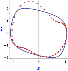
Figure 1: Comparison of limit cycles given by the approximate solution $\left(\text{\ref{SRLE RG New Sol}}\right)$ using RGM (in dotted line) with the exact numerical limit cycle (in solid line) for $\left(a\right)$ $k=0.5\ \left(\text{or }F=0.5\omega^{2}\right),\ \omega=1.15\ \left(\text{or }\varepsilon=0.75614\right),\ \sigma_{1}=0.07$ and $\left(b\right)$ $k=0.4\ \left(\text{or }F=0.4\omega^{2}\right),\ \omega=2\ \left(\text{or }\varepsilon=0.25\right),\ \sigma_{1}=0.01.$

Similarly, for

$$k=0.4,\ \omega=2,\ \sigma_{1}=0.01$$ (2.28)

so that

$$F=0.4\omega^{2}$$

we have $\varepsilon=0.25$ and $\left(\text{\ref{SRLE Freq-response Eq}}\right)$ gives three values of $\rho$ as

$$\rho=4.3722\times 10^{-2},\ 0.77347\text{ and }1.1828$$

We take the largest value $\rho=1.1824$ so that

$$\Delta=0.12105>0$$

i.e., our choice of parameters in $\left(\text{\ref{SRLE Parameter Val2}}\right)$ satisfy both the convergence criteria. The limit cycle from RG solution $\left(\text{\ref{SRLE RG New Sol}}\right)$ is represented by dotted line along with the numerically computed (exact) limit cycle represented by solid line in the Figure 1 with the values of the parameters given by $\left(\text{\ref{SRLE Parameter Val2}}\right)$.

To summarize, homotopically extended RGM is successful in reproducing qualitatively reasonable relaxation oscillation solutions when the singular problem is transformed into a regular problem but with a large value of nonlinearity parameter. In the next subsection, we show that almost analogous results are also recovered, with only minor differences in the explicit forms of the approximate solutions, by implementing an alternative homotopy variation. In subsection 2.4, we consider the forced Rayleigh problem with strong nonlinearity in the context of homotopy RGM. It is heartening to note that the limiting homotopy RGM solutions matches exactly with the formal RGM solution of Appendix, establishing, in retrospect, the strength of classical RGM even yielding qualitatively reasonable periodic solutions in a strongly nonlinear oscillation.

2.3 Homotopy and RGM: Case 2: SRLE, Alternate homotopy deformation

Let us consider the singular Rayleigh equation $\left(\text{\ref{SFRL Eqn}}\right)$ with $\varepsilon<1$, but present in the alternative form

$$\varepsilon\ddot{x}(t)+\varepsilon x\left(t\right)+\left\{\left(\frac{1}{3}\dot{x}(t)^{3}-\dot{x}(t)\right)+\left(1-\varepsilon\right)x(t)\right\}=F\varepsilon\cos(\Omega t),\ \varepsilon<1\text{.}$$ (2.29)

Motivation of this choice comes from the salient fact that the success of RGM in recovering the qualitative features of periodic oscillations basically rests on the availability of a zeroth order harmonic term in the perturbative expansion of the desired solution. Since the non-linearity term in the above equation is still large, we consider, instead the following homotopically extended system to study the limit cycle solution

$$\varepsilon\ddot{x}(t)+\varepsilon x\left(t\right)+\mu\left\{\left(\frac{1}{3}\dot{x}(t)^{3}-\dot{x}(t)\right)+\left(1-\varepsilon\right)x(t)\right\}=F\varepsilon\mu\cos(\Omega t),\ \varepsilon<1,$$ (2.30)

which becomes the forced singular problem $\left(\text{\ref{SRLE Alt Eq}}\right)$ for $\mu=1$. Next, choosing, as above,

$$\Omega=1+\mu\sigma\text{.}$$ (2.31)

one expands limit cycle solution as

$$x\left(t\right)=x_{0}\left(t\right)+\mu\ x_{1}\left(t\right)+\mu^{2}x_{2}\left(t\right)+...$$ (2.32)

so that the RG flow equations are (Appendix)

$$\frac{dR}{dt} =\frac{1}{\varepsilon}\mu\left(\frac{R}{2}-\frac{R^{3}}{8}\right)-\frac{F}{2}\mu\sin\theta+O\left(\mu^{2}\right)$$ (2.33)

$$\frac{d\theta}{dt} =1-\frac{\mu}{2R\varepsilon}\left(F\varepsilon\cos\theta+R\left(\varepsilon-1\right)\right)+O\left(\mu^{2}\right)\text{.}$$ (2.34)

The renormalized solution after taking the limit $t\rightarrow\infty$ and eliminating the secular terms is

$$x\left(t\right)=R\left(t\right)\cos\left(\theta\left(t\right)\right)+\frac{1}{96\varepsilon}\mu R^{3}\left(t\right)\sin\left(3\theta\left(t\right)\right)\text{.}$$ (2.35)

Finally, putting $\mu=1$, by continuity, in $\left(\text{\ref{SRLE Alt RG Eq1}}\right)$, $\left(\text{\ref{SRLE Alt RG Eq2}}\right)$ and $\left(\text{\ref{SRLE Alt RG Sol}}\right)$ we get,

$$\frac{dR}{dt} =\frac{1}{\varepsilon}\left(\frac{R}{2}-\frac{R^{3}}{8}\right)-\frac{F}{2}\sin\theta$$ (2.36)

$$\frac{d\theta}{dt} =\frac{1}{2}+\frac{1}{2\varepsilon}-\frac{1}{2R}F\cos\theta$$ (2.37)

and

$$x\left(t\right)=R\left(t\right)\cos\left(\theta\left(t\right)\right)+\frac{1}{96\varepsilon}R^{3}\left(t\right)\sin\left(3\theta\left(t\right)\right)\text{.}$$ (2.38)

Taking

$$\theta=\phi+\left(\frac{1}{2}+\frac{1}{2\varepsilon}+\sigma\right)\ t$$

from $\left(\text{\ref{SRLE Alt RG New Eq1}}\right)$ and $\left(\text{\ref{SRLE Alt RG New Eq2}}\right)$ we get,

$$\frac{dR}{dt} =\frac{1}{\varepsilon}\left(\frac{R}{2}-\frac{R^{3}}{8}\right)-\frac{F}{2}\sin\left(\phi+\left(\frac{1}{2}+\frac{1}{2\varepsilon}+\sigma\right)\ t\right)$$ (2.39)

$$\frac{d\phi}{dt}+\sigma =-\frac{1}{2R}F\cos\left(\phi+\left(\frac{1}{2}+\frac{1}{2\varepsilon}+\sigma\right)\ t\right)\text{.}$$ (2.40)

For steady state motion $\frac{dR}{dt}=0$ and $\frac{d\phi}{dt}=0$ so that the above equations give

$$\left(\frac{R}{2}-\frac{R^{3}}{8}\right) =\frac{F\varepsilon}{2}\sin\left(\phi+\left(\frac{1}{2}+\frac{1}{2\varepsilon}+\sigma\right)\ t\right)$$

$$R\varepsilon\sigma =-\frac{1}{2}F\varepsilon\cos\left(\phi+\left(\frac{1}{2}+\frac{1}{2\varepsilon}+\sigma\right)\ t\right)\text{.}$$

Squaring and then adding we get,

$$\frac{R^{2}}{4}\left(1-\frac{R^{2}}{4}\right)^{2}+R^{2}\varepsilon^{2}\sigma^{2}=\frac{F^{2}\varepsilon^{2}}{4}.$$

Taking

$$\rho=\frac{R^{2}}{4},\ \sigma_{1}=\varepsilon\sigma\text{ and }k=F\varepsilon$$

we get the frequency-amplitude response equation

$$\rho\left(1-\rho\right)^{2}+4\rho\sigma_{1}^{2}=\frac{k^{2}}{4},$$ (2.41)

which is identical to the equation $\left(\text{\ref{Freq-Response Eq}}\right)$ as described in the Appendix and so the region giving stable limit cycle must satisfy both the inequalities

$$\rho>\frac{1}{2}\text{ and }\Delta>0$$

in $\rho\sigma_{1}$ plane, where

$$\Delta=\frac{1}{4}\left(1-4\rho+3\rho^{2}\right)+\sigma_{1}^{2}\text{.}$$

Taking

$$k=0.5,\ \varepsilon=0.75,\ \sigma_{1}=0.07$$ (2.42)

so that

$$F=\frac{0.5}{\varepsilon}$$

$\left(\text{\ref{SRLE Alt Freq-response Eq}}\right)$ gives three values of $\rho$ as

$$\rho=7.0777\times 10^{-2},\ 0.74685\text{ and }1.1824\text{.}$$

If we take the largest value $\rho=1.1824$ then

$$\Delta=0.12105>0\text{.}$$

Therefore, this choice of the parameter values given by $\left(\text{\ref{SRLE Alt Parameter Val}}\right)$ satisfy the convergence criteria. The limit cycle from RG solution $\left(\text{\ref{SRLE Alt RG New Sol}}\right)$ is represented by dotted line along with the numerically computed (exact) limit cycle represented by solid line in the Figure 2 with the values of the parameters given by $\left(\text{\ref{SRLE Alt Parameter Val}}\right)$.

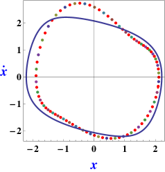
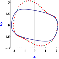
Figure 2: Comparison of limit cycles given by the approximate solution $\left(\text{\ref{SRLE Alt RG New Sol}}\right)$ using RGM (in dotted line) with the exact numerical limit cycle (in solid line) for $\left(a\right)$ $k=0.5,\ \varepsilon=0.75,\ \sigma_{1}=0.07$ and $\left(b\right)$ $k=0.4,\ \varepsilon=0.6,\ \sigma_{1}=0.07.$

Similarly, taking

$$k=0.4,\ \varepsilon=0.6,\ \sigma_{1}=0.07$$ (2.43)

so that

$$F=\frac{0.4}{\varepsilon}$$

$\left(\text{\ref{SRLE Alt Freq-response Eq}}\right)$ gives three values of $\rho$ as

$$4.2737\times 10^{-2},\ 0.83109\text{ and }1.1262.$$

Taking the largest value $\rho=1.1262$ we get

$$\Delta=7.9945\times 10^{-2}>0$$

i.e., this choice of the parameter values given by $\left(\text{\ref{SRLE Alt Parameter Val2}}\right)$ satisfy the convergence criteria. The limit cycle from RG solution $\left(\text{\ref{SRLE Alt RG New Sol}}\right)$ is represented by dotted line along with the numerically computed (exact) limit cycle represented by solid line in the Figure 2 with the values of the parameters given by $\left(\text{\ref{SRLE Alt Parameter Val2}}\right)$.

To conclude this section, we note that two alternative choices of homotopy deformations qualitatively almost identical periodic solutions c.f (2.22) and (2.38). Two solutions have almost identical forms except for minor differences in coefficients of the second terms.

2.4 Homotopy and RGM: Case 3: Regular RLE for all $\varepsilon$

In this section we consider $\left(\text{\ref{RFRL Eqn}}\right)$ for all $\varepsilon>0$. In order to study its limit cycle solution we consider the associated homotopy equation

$$\ddot{x}(t)+\varepsilon\mu\left(\frac{1}{3}\dot{x}(t)^{3}-\dot{x}(t)\right)+x(t)=F\epsilon\mu\cos(\Omega t),$$ (2.44)

which becomes the forced Rayleigh equation $\left(\text{\ref{RFRL Eqn}}\right)$ for $\mu=1$. Taking

$$\Omega=1+\mu\varepsilon\sigma$$ (2.45)

and

$$x\left(t\right)=x_{0}\left(t\right)+\mu\ x_{1}\left(t\right)+\mu^{2}x_{2}\left(t\right)+...$$ (2.46)

we get the RG flow equations

$$\frac{dR}{dt} =\mu\varepsilon\left(\frac{R}{2}-\frac{R^{3}}{8}\right)-\frac{F}{2}\mu\varepsilon\sin\theta+O\left(\mu^{2}\right)$$ (2.47)

$$\frac{d\theta}{dt} =1-\mu\frac{F}{2R}\varepsilon\cos\theta+O\left(\mu^{2}\right)$$ (2.48)

and the renormalized solution after taking the limit $t\rightarrow\infty$ and eliminating the secular terms is

$$x\left(t\right)=R\left(t\right)\cos\left(\theta\left(t\right)\right)+\frac{1}{96}\varepsilon\mu R^{3}\left(t\right)\sin\left(3\theta\left(t\right)\right)$$ (2.49)

where, $R\left(t\right)$ and $\theta\left(t\right)$ are the solutions of $\left(\text{\ref{RFRL RG Eq1}}\right)$ and $\left(\text{\ref{RFRL RG Eq2}}\right)$. Putting $\mu=1$, by continuity, in $\left(\text{\ref{RFRL RG Eq1}}\right)$, $\left(\text{\ref{RFRL RG Eq2}}\right)$ and $\left(\text{\ref{RFRL RG Sol}}\right)$ we get,

$$\frac{dR}{dt} =\varepsilon\left(\frac{R}{2}-\frac{R^{3}}{8}\right)-\frac{F}{2}\varepsilon\sin\theta$$ (2.50)

$$\frac{d\theta}{dt} =1-\frac{F}{2R}\varepsilon\cos\theta$$ (2.51)

and

$$x\left(t\right)=R\left(t\right)\cos\left(\theta\left(t\right)\right)+\frac{1}{96}\varepsilon R^{3}\left(t\right)\sin\left(3\theta\left(t\right)\right)\text{.}$$ (2.52)

As $\mu=1$ taking

$$\theta=\phi+\Omega\ t=\phi+\left(1+\varepsilon\sigma\right)t$$

in $\left(\text{\ref{RFRL RG New Eq1}}\right)$ and $\left(\text{\ref{RFRL RG New Eq2}}\right)$ we get,

$$\frac{dR}{dt} =\varepsilon\left(\frac{R}{2}-\frac{R^{3}}{8}\right)-\frac{F}{2}\varepsilon\sin\left(\phi+\Omega\ t\right)$$ (2.53)

$$\frac{d\phi}{dt}+\varepsilon\sigma =-\frac{F}{2R}\varepsilon\cos\left(\phi+\Omega\ t\right)\text{.}$$ (2.54)

For steady state motion $\frac{dR}{dt}=0$ and $\frac{d\phi}{dt}=0$, so that the above equations give

$$\left(\frac{R}{2}-\frac{R^{3}}{8}\right) =\frac{F}{2}\sin\theta$$

$$R\sigma =-\frac{F}{2}\cos\theta\text{.}$$

Squaring and then adding we get,

$$\frac{R^{2}}{4}\left(1-\frac{R^{2}}{4}\right)^{2}+R^{2}\sigma^{2}=\frac{F^{2}}{4}\text{.}$$

Taking

$$\rho=\frac{R^{2}}{4}\text{ and }k=F$$

we get the frequency-amplitude response equation as,

$$\rho\left(1-\rho\right)^{2}+4\rho\sigma^{2}=\frac{k^{2}}{4},$$ (2.55)

which is again identical to the equation $\left(\text{\ref{Freq-Response Eq}}\right)$ as described in the Appendix and so the region giving stable limit cycle must satisfy both the inequalities

$$\rho>\frac{1}{2}\text{ and }\Delta>0$$

in $\rho\sigma$ plane, where

$$\Delta=\frac{1}{4}\left(1-4\rho+3\rho^{2}\right)+\sigma^{2}\text{.}$$

Taking

$$k=F=0.5,\ \varepsilon=1.3,\ \sigma=0.07$$ (2.56)

$\left(\text{\ref{RFRL Freq-response Eq}}\right)$ gives three values of $\rho$ as

$$\rho=7.0777\times 10^{-2},\ 0.74685,\ 1.1824\text{.}$$

If we take the largest value $\rho=1.1824$ then

$$\Delta=0.12105>0\text{.}$$

Therefore, this choice of the values of the parameters given by $\left(\text{\ref{RFRL2 Parameter Val}}\right)$ satisfy both the convergence criteria. The limit cycle from RG solution $\left(\text{\ref{RFRL RG New Sol}}\right)$ is represented by dotted line along with the numerically computed (exact) limit cycle represented by solid line in the Figure 3 with the values of the parameters given by $\left(\text{\ref{RFRL2 Parameter Val}}\right)$.

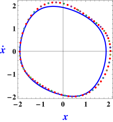
Figure 3: Comparison of limit cycles given by the approximate solution $\left(\text{\ref{RFRL RG New Sol}}\right)$ using RGM (in dotted line) with the exact numerical limit cycle (in solid line) for $\left(a\right)$ $k=F=0.5,\ \varepsilon=1.3,\ \sigma=0.07$ and $\left(b\right)\ k=F=0.4,\ \varepsilon=0.8,\ \sigma=0.06.$

Similarly, taking

$$k=F=0.4,\ \varepsilon=0.8,\ \sigma=0.06$$ (2.57)

$\left(\text{\ref{RFRL Freq-response Eq}}\right)$ gives three values of $\rho$ as

$$4.2999\times 10^{-2},\ 0.81354\text{ and }1.1435.$$

Taking the largest value $\rho=1.1435$ we get

$$\Delta=9.0794\times 10^{-2}>0$$

i.e., this choice of the parameter values given by $\left(\text{\ref{RFRL2 Parameter Val2}}\right)$ satisfy the convergence criteria. The limit cycle from RG solution $\left(\text{\ref{RFRL RG New Sol}}\right)$ is represented by dotted line along with the numerically computed (exact) limit cycle represented by solid line in the Figure 3 with the values of the parameters given by $\left(\text{\ref{RFRL2 Parameter Val2}}\right)$.

It follows that homotopy limit $\mu\rightarrow 1^{-}$ reproduces exactly the formal RGM solution as detailed in Appendix. As commented already, this demonstrates the strength of classical RGM in generating approximate periodic responses of a nonlinear system when zeroth order term happens to be harmonic, that agree qualitatively with the actual system response. However, it should be clear that there indeed is a substantial mismatch (of the order of $\sim 25\%$ or more) between the exact and the theoretically computed orbits. In the next section, we present new asymptotic results leading to quantitatively efficient approximations, thus improving the conventional setting of RGM to a more efficient theory in estimating nonlinear periodic solutions.

3 Asymptotic Duality: IRGM and Efficient Computation

By asymptotic duality [6, 8, 9], we mean an extended real analytic framework which would support identical asymptotic (limiting) $SL(2,\mathbb{R})$ invariant (viz., translation and inversion invariant) variables, that are allowed to vanish much more slowly compared to the original asymptotic variable $t$ or $t^{-1}$, as the case may be, in either of the limiting neighbourhoods $t\rightarrow 0^{+}$ or $t\rightarrow\infty$ in a nonlinear system.

To be precise, a nonlinear system is generally known to enjoy a cascade of slow scales $\tau_{n}=\varepsilon^{n}t$, so that $t$ goes to $\infty$ through scales $\varepsilon^{-n},\ \varepsilon<1$ thus activating subdominant slower scales $\tau_{n}\sim O(1)$ successively and hence leading to more and more complex evolutionary structures in the system. For a strongly nonlinear situation the relevant scales would naturally be of the form $\tau_{n}=t/\varepsilon^{n},\ \varepsilon\geq 1$ instead. Conventional asymptotic analysis such as multiple scale method, RGM etc. are known to exploit or invoke naturally such scales to convert the naive perturbation series into more effective schemes capturing non-perturbative features of the nonlinear dynamics.

However, as it becomes evident from the analysis presented in Section 2, although RGM is generally successful in capturing qualitative features of period orbits, fails indeed to yield quantitatively efficient results in strongly nonlinear problems, because of significant difference between asymptotically approximate solutions with the exact numerical orbits. Analogous limitations of multiple scale analysis can also be inferred. We note that higher order calculations based on conventional treatments can not improve the situation in a significant way, not to mention the complexity, in under taking such computations. To eliminate this limitations in conventional approaches, particularly in RGM, we propose the following [8, 9]:

In the context of a nonlinear system the conventional linear flow of time as designated above by the scales of the form $\varepsilon^{-n}$ has the potential to carry slowly varying nonlinear structures given by a renormalized, deformed scale of the form $t\sim\varepsilon^{-n}\cdot\varepsilon^{-nv(\eta)}$, where $v(\eta)\sim O(1)$ is a $SL(2,\mathbb{R})$ invariant object and $\eta\sim O(1)$ is a slow variable. To explain it more precisely and to see what is happening let us proceed in steps:

Step 1.

To introduce new asymptotic structure, let us begin by considering the set of real null and divergent (either to $\infty$ or $-\infty$) sequences, denoted $\mathcal{N}$, while $t$ being a representative divergent ( $t^{-1}$ null) sequence.

Step 2. Definitions [8, 9]

(a) The dominant characteristic scale of the nonlinear system concerned, denoted $\varepsilon$ and assumed $\varepsilon<1$, for instance, defines a null sequence $\varepsilon^{n}$, called the (primary) scale, for subsequent analysis. Relative to this scale, the asymptotic variable $t\rightarrow\infty$ gets deformed images of the form

$$t_{\pm}=\lambda_{\pm}\varepsilon^{-n}\varepsilon^{\pm nv_{\pm}(\eta)}$$ (3.1)

satisfying the inversion rule

$$t_{+}\cdot t_{-}=\lambda(\varepsilon^{-n})^{2}.$$ (3.2)

The scaling exponents $v_{\pm}(\eta)$ are, as yet unspecified real valued function of the slow variables $\tau_{n}=\varepsilon^{n}t$, that we denote, for brevity, by a general small scale $O(1)$ variable $\eta$ varying in $0<<\eta<1$ or $1<\eta<<2$. It should also become clear, from above definitions, the exponents $v_{\pm}(\eta)$ depend on the choice of the chosen scale, this will be clarified further later. Further, out of the two variables $t_{\pm}$, the smaller variable $t_{-}$ being an asymptotic one, $v(\eta)$ must respect the constraint $0<v_{-}(\eta)<1$. The proportionality parameters $\lambda_{\pm}$ and $\lambda$ are generally slowly varying functions of $\varepsilon$. Further characterization is given below.

(b) By definition,

$$v_{\pm}(\eta)=\left|\frac{\log t_{\pm}/\varepsilon^{-n}}{\log\varepsilon^{n}}\right|+o((\log\varepsilon^{-n})^{-1})$$ (3.3)

in the limit $n\rightarrow\infty$, when $\lambda_{\pm}=\mathrm{real\ const.}+o(1)$ or $o(1)$. Under this constraint, $\lambda$ itself may be slowly varying constant or vanishing. Consequently, it follows from inversion rule (3.2) that

$$v_{+}(\eta)=\ v_{-}(\eta)$$ (3.4)

hence, $v_{+}(\eta)$ must also respect the constraint $0<v_{+}(\eta)<1$. Consequently, the scaling exponents are said to be self-dual exponents and denoted by the symbol $v(\eta)\in(0,1)$. The reason for this nomenclature is explained by the following Proposition.

Proposition 1 (Duality or $SL(2,\mathbb{R})$ Invariance Properties)

[8, 9] The scaling exponents $v_{\pm}(\eta)$, denoted for brevity by $v(\eta)$, satisfy the following invariance properties.
(1) $v(k\eta)=v(\eta)$, for any constant $k$,
(2) $v(\eta^{-1})=v(\eta)$,
(3) $v(\eta-\eta_{0})=v(\eta)$, for any $\eta_{0}$ satisfying, for instance, the inequality $0<|\eta_{0}|\leq|\eta|\leq 1$, which are all valid up to an additive null sequence $o(1)$.

Proof. The proof of these invariance properties, viz., (1) Scaling, (2) Inversion and (3) Translation, follow directly from Definitions (a) and (b). However, for completeness, we sketch here the proofs of inversion and translation invariance, (2) and (3) respectively.

Proof of (2): For definiteness, we work with $t_{+}:=\tau^{-1}$ (say). Then $\tau<<1$, and the corresponding scale is $\varepsilon^{n}$. By definition (3.3),

$$v(\eta^{-1})=\left|\frac{\log\tau/\varepsilon^{n}}{\log\varepsilon^{n}}\right|+o(1)=\left|\frac{\log t_{+}/\varepsilon^{-n}}{\log\varepsilon^{n}}\right|+o(1)=v(\eta),$$ (3.5)

where $\eta^{-1}\lessapprox 1$ when $\eta\gtrapprox 1$, proving the inversion invariance. (Q.E.D.)

Proof of (3): Again, by definition (3.3)

$$v_{\pm}(\eta-\eta_{0})=\left|\frac{\log\varepsilon^{n}(t_{+}-t_{+0})}{\log\varepsilon^{n}}\right|+o(1)=\left|\frac{\log\varepsilon^{n}t_{+}}{\log\varepsilon^{n}}\right|+\left|\frac{\log(1-t_{+0}/t_{+})}{\log\varepsilon^{n}}\right|+o(1)=v(\eta)$$ (3.6)

since the second logarithmic term in second equality vanishes faster ( here $0<<t_{+0}<t_{+}$), proving the translation invariance. (Q.E.D.)   

The translation invariance also reveals the ultrametric property of the scaling exponent $v(\eta)$. Indeed $v(\eta)$ defines an ultrametric norm on the set of the asymptotic variables $\mathcal{N}$ satisfying the strong triangular property: $v(\eta+\eta_{0})\leq\max\{v(\eta),v(\eta_{0})\}$, $\eta$, $\eta_{0}$ satisfying above inequalities. For a detail proof see [8, 9].

Let us remark that the mapping $t\mapsto v(\eta)$ can be interpreted as a renormalization group action, assigning a finite slowly varying value $v(\eta)$ to a diverging or null sequence (i.e. $t$ or $t^{-1}$). The scaling exponent $v(\eta)$ could therefore be referred either as the renormalized scaling exponent or the deformation scaling factor.

Step 3. Self-dual vis-$\acute{a}$-vis Trivial Ultrametric

The stronger triangular inequality satisfied by the self dual exponent $v(\eta)$ tells that $v(\eta)$ acts on $\mathcal{N}$ as an ultrametric norm. Under such ultrametric norm the asymptotic set $\mathcal{N}$ naturally has the structure of a totally disconnected set, while the value set of the norm $v(\eta)$ can at most be countable [30]. The particular norm that specifies a constant $O(1)$ value to each element of $\mathcal{N}$ is the trivial ultrametric. It also follows in the present context that this trivial norm, by its very definition, is self dual. This ultrametric norm is constant over the set $\mathcal{N}$, but could indeed be a function on slow variables characteristic of the given nonlinear system. Consequently, the self dual norm $v(\eta)$ is a trivial ultrametric norm over $\mathcal{N}$ when the proportionality parameter $\lambda$ in the inversion rule (3.2) is a slowly varying constant.

Incidentally, we remark that depending on the choice of a scale $\delta$ (say), the self dual exponent $v(\eta)$ could be extended to more general duality relations, viz., (1) weakly self dual (or simply dual) exponents $v_{+}(\eta)=\alpha(\delta)v_{-}(\eta),\ \alpha(\delta)>0$, when $\lambda$ in (3.2) is slowly varying as $O((\log\delta)^{k})$, $k$ a constant, and strictly dual when $v_{+}(\eta)v_{-}(\eta)=\mu(\delta),\mu>0$ and $\lambda$ in (3.2) is slowly varying as $O(\delta^{\kappa})$, $\kappa$ a constant [9]. Parameters such $\alpha$, $\mu$ etc. appearing in above definitions can also be slowly varying following various possible patterns that could be discerned in a specific nonlinear problem. Possible applications of weakly dual and strictly dual cases would be considered in the context of period doubling bifurcations in nonlinear oscillations in subsequent works.

Step 4. Analytic Function Space

The space of periodic solutions of nonlinear oscillations consists, in general, of analytic functions. One needs to specify the action of the ultrametric scaling exponents on the space of analytic functions. This would later facilitate one to improve upon the RGM approximate solutions of limit cycle solutions to an efficient computation.

Let $(x(t),y(t)),\ y(t)=\dot{x}(t)$ be the exact phase space solution of the nonlinear periodic orbit and $(x_{0}(t),y_{0}(t))$ be the corresponding RGM approximation. Recalling from Section 2 the fact that an approximate periodic solution is retrieved from naive perturbation series following RG algorithms in the limit $t\rightarrow\infty$ through linear scales of $\varepsilon^{-n}$, when amplitude and phase flow equations attain stationary condition. Let $t_{0}=k\varepsilon^{-n}$ be a sufficiently large time instant. In a numerical computation one usually replaces $\infty$ by $t_{0}$ for $n$ sufficiently large.

In the context of the so-called IRGM, we introduce nonlinear deformation in the above linear flow of time through self dual scaling exponent $v(\eta)$ and replace the large time instance $t_{0}$ instead by $T_{0}=t_{0}\cdot t_{0}^{-v(\eta)}$. For a sufficiently small, but nevertheless $O(1)$, $v(\eta)$, the linearized deformed time has the form $T_{0}=t_{0}-v(\eta)t_{0}\log t_{0}:=t_{0}+\chi(\eta)$.

Now, there is a caveat here. We make an important comment on the nature of time scale deformations in the context of a dynamical system.

Step 4.1. Dynamical time scale

A nonlinear system generally involves multiple characteristic scales. A periodic oscillation in a slow-fast system such as singularly perturbed Rayleigh equation is characterized by the presence of vary fast and slow rates of motion along two independent phase space directions [2, 15]. Consequently, the deformation factor, considered for the time scale $t_{0}$, viz., $t_{0}^{-v(\eta)}$ involving only one deformation exponent $v(\eta)$ is too restrictive, and frozen, so to speak, in character. To allow for a more flexible and dynamic character accommodating different rates of evolution, one may introduce, in the following, more general dynamical deformation scales given by $\sigma(t_{0}):=t_{0}^{-1/\psi(t_{0})}$, so that the scale dependent $SL(2,\mathbb{R})$ deformation exponent is now given by

$$v_{\psi}(\eta)=\left|\frac{\log T_{0}/t_{0}}{\log\sigma}\right|+O(1)$$ (3.7)

where $\psi(t_{0})\geq 0$ is, in general, an analytic function, depending only on the phase space variables $x,\ y,\ldots$. The deformation scale is dynamic, as the factor $\sigma$ accommodates naturally any critical behaviour that a system may experience, by dynamically adjusting or expanding the original scale $t_{0}$ to a more larger scale, specific to the system behaviour, close to a critical point (set) satisfying $\dot{x}=0$, or $\dot{y}=0$ etc. In the present nonlinear oscillation problem (slow-fast system), as detailed in the following, we choose to work with $\psi_{x}:=k_{x}^{-1}|\dot{x}_{0}|t_{0}\log t_{0}$ and $\psi_{y}:=k_{y}^{-1}|\dot{y}_{0}|t_{0}\log t_{0}$, for some positive constants $k_{i},\ i=x,y$, where $x_{0}$ and $y_{0}$ are the RGM approximated solutions of $x$ and $y$.

The above choice is guided by the above mentioned property of slow fast systems involving different rates of oscillatory motion. As it turns out, such choices along $x$ and $y$ directions could successfully yield very high level of precision computations, exceeding $98\%$ or above accuracy level. More interestingly, one expects a sort of visual (graphical) verification of slow fast action of the the dynamic scales in the form of a condensation and rarefaction phenomenon in the distribution of data points along the fast and slow phase paths respectively, in a numerical application of the method in a relaxation oscillation. In the next section, we indeed get explicit verifications of this sort of condensation and rarefaction phenomenon in the phase diagrams of periodic orbits. One notes also that the corresponding nonlinear, dynamically deformed time, denoted as $T_{0}^{\psi}$, has the form

$$T_{0}^{\psi}=t_{0}-v_{\psi}(\eta)t_{0}\log\sigma(t_{0}):=t_{0}+\frac{v_{\psi}(\eta)}{\psi(t_{0})}t_{0}\log t_{0}:=t_{0}+\chi_{\psi}(t_{0},\eta).$$ (3.8)

Next, turning back to our discussion of analytic functions, we replace approximate solution $(x_{0}(t),y_{0}(t))$ by corresponding dynamically deformed solution $\tilde{x}_{0}=x_{0}(t_{0}+\chi_{x}(t_{0},\eta))$ and $\tilde{y}_{0}=y_{0}(t_{0}+\chi_{y}(t_{0},\eta))$, where $\chi_{i}(t_{0},\eta)=\frac{v_{\psi}(\eta)}{\psi_{i}(t_{0})}t_{0}\log t_{0},\ i=x,y$. Assuming analyticity of the solutions one then gets the linearized solutions as

$$\tilde{x}_{0}=x_{0}(t_{0})+\dot{x}_{0}(t_{0})\chi_{x}(t_{0},\eta),\ \tilde{y}_{0}=y_{0}(t_{0})+\dot{y}_{0}(t_{0})\chi_{y}(t_{0},\eta).$$

The precise mismatch between the exact and approximated solutions in IRGM is now estimated as

$$x(t_{0})-x_{0}(t_{0}) =\dot{x}_{0}(t_{0})\chi_{x}(\eta)=k_{x}v_{x}(\eta),$$ (3.9)

$$y(t_{0})-y_{0}(t_{0}) =\dot{y}_{0}(t_{0})\chi_{y}(\eta)=k_{y}v_{y}(\eta)$$ (3.10)

when we fix the dynamical scales along $x$ and $y$ directions as $\psi_{x}:=k_{x}^{-1}|\dot{x}_{0}|t_{0}\log t_{0}$ and $\psi_{y}:=k_{y}^{-1}|\dot{y}_{0}|t_{0}\log t_{0}$ respectively, for some positive adjustable constants $k_{x}$ and $k_{y}$.

We next invoke analyticity of the scaling exponents $v_{x}$ and $v_{y}$ and then may approximate $v_{i}(\eta),\ i=x,y$ by polynomials $v_{i}(\eta)=\sum_{1}^{m}a_{ij}\eta^{j},\ i=x,y$. One then specifies the constants $a_{ij}$ and free parameters $k_{i}$ so as to obtain best fit approximations of $v_{i}(\eta)$, leading to high precision periodic solution by IRGM. However, as it will become evident, single piece polynomial approximation may not be sufficient to yield efficient matching of orbits. One indeed requires multi-component polynomial functions for $v_{i}$s over a complete period of oscillation, to yield an efficient computation. Since we are presenting our computational results using the state of art computational platform of Mathematica, the question of assuring smoothness at the boundary (branch) points where two best fitted polynomials are supposed to match smoothly, so as to yield a smooth function on the entire period of the periodic oscillation concerned, could not be tackled in the present paper. To address this problem fully, one perhaps needs to invoke independent code, that we leave for future work, though, theoretically, determining smoothly matched best fit polynomial curves across boundary points should not be difficult with so many available adjustable parameters. We close this section with the following observation.

The multi-component polynomial best fit estimations of correction terms $V_{i}(\eta)$ in (3.9) and (3.10) correspond to best possible piece-wise analytic approximations of the residual periodic functions $x(t_{0})-x_{0}(t_{0})$ and $y(t_{0})-y_{0}(t_{0})$ respectively, that arise from inaccurate approximations of exact solutions in the conventional asymptotic techniques. The identification and efficient estimations of these residual inaccuracies may be considered as significant advances in the context of the present formalism.

4 Examples: Efficient estimation of relaxation cycles

To establish and demonstrate the significance of IRGM accommodating novel asymptotic structures, we now present the main steps of numerical calculations, with corresponding graphical representations, for Example (A) singularly perturbed Rayleigh equation $\left(\text{\ref{SFRL Eqn}}\right)$ and Example (B) ( regular) Rayleigh equation $\left(\text{\ref{RFRL Eqn}}\right)$ with a large nonlinearity parameter $\varepsilon>1$. We refer to Section 2.2 and 2.4 for the homotopy aided RGM computed solutions of these two cases.

Example A

The RG solution after putting $\mu=1$ for the singular equation $\left(\text{\ref{SFRL Eqn}}\right)$ is given by $\left(\text{\ref{SRLE RG Sol}}\right)$. In Figure 1 we see that the exact limit cycle and its approximation by RGM are significantly different (i.e. accuracy not exceeding $75\%$) for $F=0.4,$ $\omega=2\ \left(\text{or }\varepsilon=0.25\right)$, $\sigma=0.01\omega^{2}$.

To improve upon the above limitations, we first fix slower $O(1)$ variable $\eta$ that is supposed to appear in the scaling exponents of (3.9). For $\varepsilon=0.25$, by observation, one finds a complete oscillation of the relaxation cycle concerned in the time interval $190<t<200$, and the minimum value of $n$ so that $\eta=\varepsilon^{n}t$ falls in $(0,1)$ is $n=4$. Indeed, one verifies that for complete period $190<t<200$, the slow variable $\eta$ satisfies $0.7421875<\eta<0.78125$ for $n=4$.

Next, one notes a phase difference between the numerically computed solution $x(t)$ and the RGM solution $x_{0}(t)$ in the said interval (Figure 4).

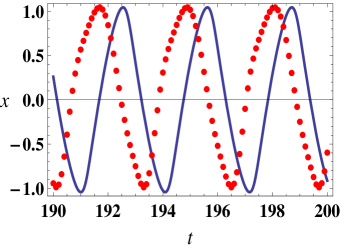
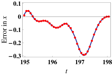
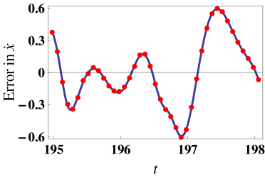
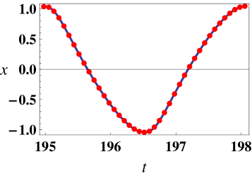
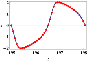
Figure 4: Improving the approximation shown in Figure 1 discussed in Section 2.2. Here Solid lines represent exact solutions and Dotted lines represent approximate solutions.
$\left(a\right)$ Comparison of the exact solution $x\left(t\right)$ of $\left(\text{\ref{SFRL Eqn}}\right)$ and the RGM approximation given by $\left(\text{\ref{SRLE RG Sol}}\right)$ for $190<t<200.$ $\left(b\right)$ Comparison of $x\left(t+0.65\right)$ and the RGM approximation given by $\left(\text{\ref{SRLE RG Sol}}\right)$ showing better agreement for $190<t<200$. $\left(c\right)$ Comparison of exact error $x\left(t+0.65\right)-x_{0}\left(t\right)$ and its estimate of $\psi_{x}\left(t\right)$ given by $\left(\text{\ref{Error1 Estimate in x}}\right)$ in $\left[r_{1},r_{3}\right]$. $\left(d\right)$ Comparison of exact error $\dot{x}\left(t+0.65\right)-\dot{x}_{0}\left(t\right)$ and its estimate of $\psi_{y}\left(t\right)$ given by $\left(\text{\ref{Error1 Estimate in y}}\right)$ in $\left[r_{1},r_{3}\right]$. $\left(e\right)$ Comparison of $x\left(t+0.65\right)$ and its estimate $x_{0}\left(t\right)+\psi_{x}\left(t\right)$. $\left(f\right)$ Comparison of $\dot{x}\left(t+0.65\right)$ and its estimate $\dot{x}_{0}\left(t\right)+\psi_{y}\left(t\right)$.

To compensate the phase difference, that is essential for determination of numerical accuracy of the technique, we verify that a suitable time translated $x(t)\rightarrow x(t+0.65)$ have approximately identical phase with $x_{0}(t)$, viz., (Figure 4)

$$x\left(t+0.65\right)\approx x_{0}\left(t\right),$$

in phase. It turns out that this time translation along $x$ direction is inherited by $y$ curves, viz., $y(t+0.65)$ and $y_{0}(t)$, both having almost identical phases. This suffices us to replace $\left(\text{\ref{error}}\right)$ and $\left(\text{\ref{error in y}}\right)$ by new phase shifted error equations

$$x(t+0.65)-x_{0}(t) =\dot{x}_{0}(t)\chi_{x}(\eta)=k_{x}v_{x}(\eta)\equiv\psi_{x}(t),$$ (4.1)

$$y(t+0.65)-y_{0}(t) =\dot{y}_{0}(t)\chi_{y}(\eta)=k_{y}v_{y}(\eta)\equiv\psi_{y}(t),$$ (4.2)

where $\eta=\varepsilon^{n}t$ for $190<t<200,\ \varepsilon=0.25,\ n=4$ using best fit polynomial curves as follows.

In order to identify the period of the oscillation, we find that $x\left(t+0.65\right)$ $\left(\text{not }x_{0}\left(t\right)\right)$ has successive maximum at the points $r_{1}=194.975,\ r_{3}=198.055$ and it has a minimum in between them at $r_{2}=196.515$ in the interval $190<t<200$. Thus, the period of the function $x\left(t+0.65\right)$ is $T=r_{3}-r_{1}=198.055-194.975=3.08\text{. }$The graph of $x\left(t+0.65\right)-x_{0}\left(t\right)$ is shown in Figure 4 on $\left[r_{1},r_{3}\right]$ through solid line. It is difficult to estimate the above function using a single polynomial. So, by careful observation we divide the interval $\left[r_{1},r_{3}\right]$ into subintervals

$$\left[r_{1},195.7\right],\ \left[195.7,196.6\right],\ \left[196.6,197.6\right],\ \left[197.6,r_{3}\right]$$

and then estimate them using $100$ equidistant data points from each subintervals through Mathematica by the piecewise function (expected to be continuous and smooth, but yet to be verified (c.f. Section 3, item 4.1, remarks on error estimation))

$$\psi_{x}\left(t\right)=\left\{\begin{array}[c]{ll}-6.08565\times 10^{9}+1.2456\times 10^{8}t-956058.t^{2}+3261.41t^{3}-4.17212t^{4},&r_{1}\leq t\leq 195.7\\ -3.44505\times 10^{9}+7.02609\times 10^{7}t-537357.t^{2}+1826.54t^{3}-2.32822t^{4},&195.7<t\leq 196.6\\ -4.11615\times 10^{9}+8.35121\times 10^{7}t-635386.t^{2}+2148.53t^{3}-2.72444t^{4},&196.6<t\leq 197.6\\ -563206+5648.14t+0.153819t^{2}-0.143543t^{3}+0.000359855t^{4},&197.6<t\leq r_{3}\end{array}\right.$$ (4.3)

the graph of which is shown in the Figure 4 through dotted line. Similarly,

$$\psi_{y}\left(t\right)=\left\{\begin{array}[c]{ll}-8.09646\times 10^{10}+1.24433\times 10^{9}t-4.25298\times 10^{6}t^{2}-21721.8t^{3}+167.046t^{4}-0.285255t^{5},&r_{1}\leq t\leq 195.5\\ -9.50313\times 10^{9}+1.45469\times 10^{8}t-494748.t^{2}-2526.17t^{3}+19.3312t^{4}-0.0328788t^{5},&195.5<t\leq 196.3\\ -4.16274\times 10^{10}+6.35172\times 10^{8}t-2.15314\times 10^{6}t^{2}-10963.2t^{3}+83.6184t^{4}-0.141766t^{5},&196.3<t\leq 196.85\\ 1.5638\times 10^{10}-2.37679\times 10^{8}t+802502.t^{2}+4071.01t^{3}-30.9271t^{4}+0.0522281t^{5},&196.85<t\leq 197.7\\ 3.24289\times 10^{7}-327797.t+0.102438t^{2}+8.37216t^{3}-0.0211569t^{4},&197.7<t\leq r_{3}\end{array}\right.$$ (4.4)

the graph of which is compared with the exact error $\dot{x}\left(t+0.65\right)-\dot{x}_{0}\left(t\right)$ in the Figure 4. The graphs of $x\left(t+0.65\right)$, $\dot{x}\left(t+0.65\right)$ and their respective estimates $x_{0}\left(t\right)+\psi_{x}\left(t\right)$, $\dot{x}_{0}\left(t\right)+\psi_{y}\left(t\right)$ are shown in Figure 4 and Figure 4 respectively.

To estimate the percentage error in above numerical calculations we cannot use the standard error formula, for instance, in $x$ direction

$$\max\frac{x\left(t+0.65\right)-\left(x_{0}\left(t\right)+\psi_{x}\left(t\right)\right)}{x\left(t+0.65\right)}\times 100\text{ for }r_{1}\leq t\leq r_{3}$$

for the fact that $x\left(t+0.65\right)$ may vanish in $\left[r_{1},r_{3}\right]$. So we estimate the error with respect to the amplitude $\tilde{a}$ of $x$ using the formula

$$E_{x}=\max\frac{x\left(t+0.65\right)-\left(x_{0}\left(t\right)+\psi_{x}\left(t\right)\right)}{\tilde{a}}\times 100\text{ for }r_{1}\leq t\leq r_{3}.$$ (4.5)

We find that

$$\tilde{a}=\max_{r_{1}\leq t\leq r_{3}}\left|x\left(t+0.65\right)\right|=1.04367\text{ and }\max_{r_{1}\leq t\leq r_{3}}\left\{x\left(t+0.65\right)-\left(x_{0}\left(t\right)+\psi_{x}\left(t\right)\right)\right\}=0.0127652$$

so that

$$E_{x}=\frac{0.0127652}{1.04367}\times 100=1.22\%$$

and hence we achieve an accuracy of $\left(100-E_{x}=\right)\ 98.78\%$ in this estimation.

Similarly, for estimation of $y\left(t+0.65\right)=\dot{x}\left(t+0.65\right)$ by $\dot{x}_{0}\left(t\right)+\psi_{y}\left(t\right)$ we use the formula for percentage error as

$$E_{y}=\max\frac{\dot{x}\left(t+0.65\right)-\left(\dot{x}_{0}\left(t\right)+\psi_{y}\left(t\right)\right)}{\tilde{b}}\times 100\text{ for }r_{1}\leq t\leq r_{3},$$ (4.6)

where $\tilde{b}$ is the amplitude of $\dot{x}\left(t+0.65\right)$ in $\left[r_{1},r_{3}\right]$ i.e.,

$$\tilde{b}=\max_{r_{1}\leq t\leq r_{3}}\left|\dot{x}\left(t+0.65\right)\right|\text{.}$$

Here,

$$\tilde{b}=2.02533\text{ and }\max_{r_{1}\leq t\leq r_{3}}\left\{\dot{x}\left(t+0.65\right)-\left(\dot{x}_{0}\left(t\right)+\psi_{y}\left(t\right)\right)\right\}=0.0311104$$

so that

$$E_{y}=\frac{0.0311104}{2.02533}\times 100=1.54\%$$

and hence we achieve an accuracy of $\left(100-E_{y}=\right)\ 98.46\%$ in this estimation. The estimated limit cycle with $x_{0}\left(t\right)+\psi_{x}\left(t\right)$ and $\dot{x}_{0}\left(t\right)+\psi_{y}\left(t\right)$ is compared with exact limit cycle in Figure 5.

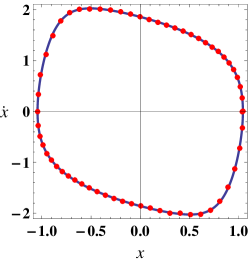
Figure 5: The solid line represents numerically computed exact limit cycle as discussed in Section 2.2 and the dotted line represents the estimated limit cycle by $x_{0}\left(t\right)+\psi_{x}\left(t\right)$ and $\dot{x}_{0}\left(t\right)+\psi_{y}\left(t\right)$.

Example B

Next, we present efficient computations in the context of the Rayleigh Equation with large nonlinearity $\varepsilon>1$. The homotopy RG solution of Section 2.4, after putting $\mu=1$, is given by $\left(\text{\ref{RFRL RG New Sol}}\right)$. As usual, the exact limit cycle and its approximation by homotopy RGM (Figure 3) are significantly different (accuracy level being less than $75\%$) for $F=0.5,$ $\varepsilon=1.3$, $\sigma=0.07$.

Now, following the steps of (A), for a complete cycle we choose $185<t<200$, so that the minimum value of $n$ is now fixed at $n=21$ and the slow variable $\eta=\varepsilon^{-21}t\in\left(0,1\right)$, for $\varepsilon=1.3$. In order to remove relative phase difference between exact and approximated solution, one time translates the exact solution $x(t)\rightarrow x(t+2.7)$, and consider the phase corrected error equations in the form

$$x(t+2.7)-x_{0}(t) =\dot{x}_{0}(t)\chi_{x}(\eta)=k_{x}v_{x}(\eta)\equiv\tilde{v}_{x}(\eta)=\psi_{x}(t),$$ (4.7)

$$y(t+2.7)-y_{0}(t) =\dot{y}_{0}(t)\chi_{y}(\eta)=k_{y}v_{y}(\eta)\equiv\tilde{v}_{y}(\eta)=\psi_{y}(t),$$ (4.8)

where $\eta=\varepsilon^{-21}t$ for $185<t<200,\ \varepsilon=1.3,$ using multi-component polynomial curve fitting. As before, we estimate the period of $x\left(t+2.7\right)$ as $T=r_{3}-r_{1}=5.759$, where the maxima of the oscillation are attained at $r_{1}=190.507,\ r_{3}=196.266$, when the minimum value is at $r_{2}=193.387$ for $185<t<200$.

Thereafter, we use here three piece polynomial fitting to annul the error difference in (4.7) as

$$\psi_{x}\left(t\right)=\left\{\begin{array}[c]{ll}-7.29799\times 10^{7}+1.51571\times 10^{6}t-11804.4t^{2}+40.8578t^{3}-0.0530298t^{4},&r_{1}\leq t\leq 191.9\\ -1.42254\times 10^{8}+2.9514\times 10^{6}t-22962.5t^{2}+79.4005t^{3}-0.102957t^{4},&191.9<t\leq 194\\ -2.38474\times 10^{8}+4.893\times 10^{6}t-37647.7t^{2}+128.74t^{3}-0.165089t^{4},&194<t\leq r_{3}.\end{array}\right.$$ (4.9)

Similarly, one estimates $\dot{x}\left(t+2.7\right)$ using $\dot{x}_{0}\left(t\right)+\psi_{y}\left(t\right)$ by dividing the interval $\left[r_{1},r_{3}\right]$ instead in four subintervals and then estimated $\dot{x}\left(t+2.7\right)-\dot{x}_{0}\left(t\right)$ by the piecewise function

$$\psi_{y}\left(t\right)=\left\{\begin{array}[c]{cl}-3.48561\times 10^{9}+7.29408\times 10^{7}t-572390.t^{2}+1996.32t^{3}-2.61094t^{4},&r_{1}\leq t\leq 191.6\\ -6.14729\times 10^{8}+1.27786\times 10^{7}t-99611.6t^{2}+345.106t^{3}-0.448357t^{4},&191.6<t\leq 193.4\\ 2.1483\times 10^{9}-4.43429\times 10^{7}t+343228.t^{2}-1180.75t^{3}+1.52322t^{4},&193.4<t\leq 194.6\\ 7.30449\times 10^{8}-1.4952\times 10^{7}t+114771.t^{2}-391.545t^{3}+0.500907t^{4},&194.6<t\leq r_{3}.\end{array}\right.$$ (4.10)

The graph of $x\left(t+2.7\right)$, $\dot{x}\left(t+2.7\right)$ and their respective estimates $x_{0}\left(t\right)+\psi_{x}\left(t\right)$, $\dot{x}_{0}\left(t\right)+\psi_{y}\left(t\right)$ are shown in Figure 6.

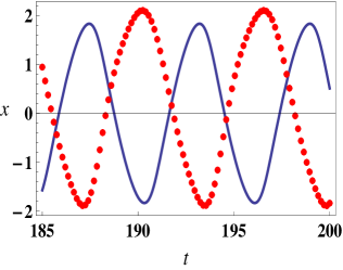
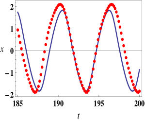
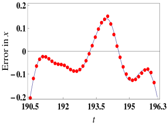
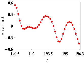
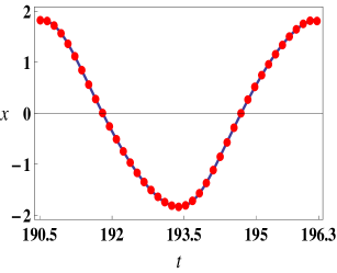
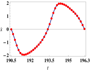
Figure 6: Improving the approximation shown in Figure 3 discussed in Section 2.4. Here Solid lines represent exact solutions and Dotted lines represent approximate solutions.
$\left(a\right)$ Comparison of the exact solution $x\left(t\right)$ of $\left(\text{\ref{RFRL Eqn}}\right)$ and the RGM approximation given by $\left(\text{\ref{RFRL RG New Sol}}\right)$ for $185<t<200.$ $\left(b\right)$ Comparison of $x\left(t+2.7\right)$ and the RGM approximation given by $\left(\text{\ref{RFRL RG New Sol}}\right)$ showing better agreement for $185<t<200$. $\left(c\right)$ Comparison of exact error $x\left(t+2.7\right)-x_{0}\left(t\right)$ and its estimate of $\psi_{x}\left(t\right)$ given by $\left(\text{\ref{Error2 Estimate in x}}\right)$ in $\left[r_{1},r_{3}\right]$. $\left(d\right)$ Comparison of exact error $\dot{x}\left(t+2.7\right)-\dot{x}_{0}\left(t\right)$ and its estimate of $\psi_{y}\left(t\right)$ given by $\left(\text{\ref{Error2 Estimate in y}}\right)$ in $\left[r_{1},r_{3}\right]$. $\left(e\right)$ Comparison of $x\left(t+2.7\right)$ and its estimate $x_{0}\left(t\right)+\psi_{x}\left(t\right)$. $\left(f\right)$ Comparison of $\dot{x}\left(t+2.7\right)$ and its estimate $\dot{x}_{0}\left(t\right)+\psi_{y}\left(t\right)$.

As in Example A, we next estimate percentage errors along $x$ and $y$ directions as $E_{x}=1.26\%$ and $E_{y}=1.08\%$ where $\tilde{a}=\max_{r_{1}\leq t\leq r_{3}}\left|x\left(t+2.7\right)\right|=1.83249,\text{ and }\ \max_{r_{1}\leq t\leq r_{3}}\left\{x\left(t+2.7\right)-\left(x_{0}\left(t\right)+\psi_{x}\left(t\right)\right)\right\}=0.0230739$, and similarly for $E_{y}$, and hence accuracy of $O(98.74\%)$ and $O(98.92\%)$ is achieved along $x$ and $y$ directions respectively. The estimated limit cycle with $x_{0}\left(t\right)+\psi_{x}\left(t\right)$ and $\dot{x}_{0}\left(t\right)+\psi_{y}\left(t\right)$ is compared with exact limit cycle in Figure 7.

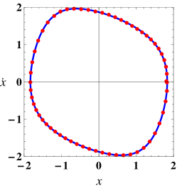
Figure 7: The solid line represents numerically computed exact limit cycle as discussed in Section 2.4 and the dotted line represents the estimated limit cycle by $x_{0}\left(t\right)+\psi_{x}\left(t\right)$ and $\dot{x}_{0}\left(t\right)+\psi_{y}\left(t\right)$.

4.1 Discussion and Comparison

The above two examples clearly demonstrate the role and significance of dynamical time scales (3.7) introduced along $x$ and $y$ in the phase plane. In Figure 4 - Figure 7, one clearly notices the distributions of estimated data points undergoing a process of condensations and rarefactions over specific intervals along the time axis that correspond to slow and fast motions in the relaxation oscillation concerned. In Figure 5, in particular, the branch of relaxation oscillation undergoing slow building up accommodates more data points, when a sparser set of data points is presented along the branch as the system relaxes very fast. This fact is demonstrated explicitly in Figures 4-4 presenting different error estimates relevant for the relaxation oscillation of Figure 5. One notices clearly denser set of data points in the neighbourhood of $t=196$ and a sparser set near $t=197$ in all these four figures. Similar condensations and rarefactions are also observed near $t=198$ and $t=195$ respectively, reflecting periodicity of the original orbit. Similar behaviours are also observed in Figure 6 and Figure 7. Such oscillations in the density of estimated data points involving dynamical time scales along independent phase space variables may be considered as an interesting novel aspect of the present asymptotic formalism. The very high level of efficiency, defined by $\left(\text{\ref{effx}}\right)$ and $\left(\text{\ref{effy}}\right)$, is obtained by a very simple computational scheme, developed in the present formalism based, however, on some novel dynamical insights, has the added advantage of visual demonstrations of the existence of slow fast motions in the nonlinear oscillations. The present study is a specific application of the nonlinear $SL\left(2,\mathbb{R}\right)$ asymptotic analysis which, in fact, have a wider range of applications [6, 7, 8, 9] and philosophical implications [24]. The computations presented involve only a few $($actually one or two only$)$ harmonic terms when conventional approaches based on either homotopy analysis method [12] or generalized averaging method etc. [22, 15] require $10$ or more harmonic terms to attain equivalent level of efficiency (accuracy).

5 Conclusion

The novel framework of $SL(2,\mathbb{R})$ invariant asymptotic structures is presented in the context of a nonlinear oscillatory system. The significance and nontrivial applications of these asymptotic structures are explained for evaluating highly efficient phase portraits (accuracy level exceeding $98\%$) of period 1 relaxation cycles of strongly nonlinear and singularly perturbed Rayleigh equations with periodic external forcing. We argue that $SL(2,\mathbb{R})$ asymptotic structures is powerful enough to upgrade standard RG computations on nonlinear orbits into highly efficient computations. New asymptotic structures are introduced by implementing continuous deformation of conventional linear slow scales such as $t_{n}=\varepsilon^{n}t,\ 0<\varepsilon<1$ into nonlinear dynamic scales of the form $T_{n}=t_{n}\sigma(t_{n})$, for a nonlinear deformation factor $\sigma(t_{n})$ respecting some well defined $SL(2,\mathbb{R})$ constraints. The concept and role of $(i)$ self dual deformation exponents as well as $(ii)$ its extension to dynamic time scale deformations in a slow -fast system involving very slow and very fast evolutionary directions, are explained in detail in the context of efficient computations of period 1 relaxation oscillations. The formalism presented here is robust and has a wider field of mathematical and other applications [24]. Application of the formalism to more general dually related deformation exponents will be considered separately in addressing period doubling bifurcations to chaos systematically for nonlinear oscillatory problems.

Appendix

It is known that the forced Rayleigh equation $\left(\text{\ref{RFRL Eqn}}\right)$ has a unique limit cycle around the critical point $\left(0,0\right)$ in the $x,\dot{x}$ phase plane. So, the shape of the limit cycle does not depend on the initial condition for the system $\left(\text{\ref{RFRL Eqn}}\right)$. Thus, for the sake of completeness we choose the initial condition

$$x\left(t_{0}\right)=\alpha,\ \dot{x}\left(t_{0}\right)=\beta$$ (5.1)

where, $\left(\alpha,\beta\right)\neq\left(0,0\right)$. We are trying to find limit cycle solution when the frequency $\Omega$ of the external periodic force is close to the frequency of the system. Therefore, we assume

$$\Omega=1+\varepsilon\sigma,\ \varepsilon>0$$ (5.2)

and the limit cycle solution can be written as the perturbative series

$$x\left(t\right)=x_{0}\left(t\right)+\varepsilon\ x_{1}\left(t\right)+\varepsilon^{2}x_{2}\left(t\right)+\cdots\text{.}$$ (5.3)

Using $\left(\text{\ref{Resonant Frequency}}\right)$ and $\left(\text{\ref{Pert}}\right)$ in $\left(\text{\ref{RFRL Eqn}}\right)$ and comparing coefficients of different orders of $\varepsilon$ we obtain the following equations.

Zero-th Order $$:\ddot{x}_{0}(t)+\omega^{2}x_{0}(t)=0\text{ with }x\left(t_{0}\right)=\alpha,\ \dot{x}\left(t_{0}\right)=\beta,$$ (5.4a)

$$\varepsilon\text{ Order} :\ddot{x}_{1}(t)+\omega^{2}x_{1}(t)+\frac{1}{3}\left(\dot{x}_{0}(t)\right){}^{3}-\dot{x}_{0}(t)-F\cos\omega t=0,\quad x_{1}\left(t_{0}\right)=0,\ \dot{x}_{1}\left(t_{0}\right)=0,$$ (5.4b)

$$\varepsilon^{2}\text{ Order} :\ddot{x}_{2}(t)+\omega^{2}x_{2}(t)+\dot{x}_{1}(t)\left(\dot{x}_{0}(t)\right){}^{2}-\dot{x}_{1}(t)+F\ t\ \sigma\sin\omega t=0,\text{\quad}x_{2}\left(t_{0}\right)=0,\ \dot{x}_{2}\left(t_{0}\right)=0,$$ (5.4c)

$$\cdots\ \cdots\ \cdots\ \cdots\qquad\cdots\ \cdots\ \cdots\ \cdots\qquad\cdots\ \cdots\ \cdots\ \cdots\qquad\cdots\ \cdots\ \cdots\ \cdots$$

The general solution of the zero-th order equation $$\left(\text{\ref{Order Zero DE}}\right)$$ can be written as

$$x_{0}\left(t\right)=Ae^{i\left(t-t_{0}\right)}+A^{\ast}e^{-i\left(t-t_{0}\right)},$$ (5.5)

where $A$ is a complex constant. Although $A$ can be determined from the initial conditions, we keep $A$ undetermined because the computational steps in the RGM will ultimately replace $A$ by its counterpart $\mathcal{A}$, which will not remain a constant of motion. The solution of the $\varepsilon$ order equation $\left(\text{\ref{Order One DE}}\right)$ is

$$x_{1}\left(t\right)=\left(\frac{1}{24}iA^{3}+\frac{1}{2}\left(A-A^{2}A^{\ast}\right)\left(t-t_{0}\right)-\frac{F\ i}{4}\left(t-t_{0}\right)\right)e^{i\left(t-t_{0}\right)}-\frac{1}{24}iA^{3}e^{3i\left(t-t_{0}\right)}+c.c.$$ (5.6)

where $c.c.$ designates the complex conjugate of the preceding expression. Similarly, we can continue to higher order solution to generate the naive perturbative solution of the system $\left(\text{\ref{RFRL Eqn}}\right)$.

In the second step of the RGM, we renormalize the integration constant $A$ and create a counterpart $\mathcal{A}$ as

$$A=\mathcal{A+}a_{1}\mathcal{\varepsilon}+a_{2}\varepsilon^{2}+\cdots$$

where, the coefficients $a_{1}$, $a_{2}$, … are chosen to absorb the homogeneous parts of the solution in different orders of $\varepsilon$. Choosing

$$a_{1}=-\dfrac{1}{24}i\mathcal{A}^{3}$$ (5.7)

we get,

$$x\left(t\right)=\mathcal{A}e^{i\left(t-t_{0}\right)}+\varepsilon\left\{\dfrac{1}{2}\left(\mathcal{A}-\mathcal{A}^{2}\mathcal{A}^{\ast}\right)\left(t-t_{0}\right)e^{i\left(t-t_{0}\right)}-\dfrac{F\ i}{4}\left(t-t_{0}\right)e^{i\left(t-t_{0}\right)}-\dfrac{1}{24}i\mathcal{A}^{3}e^{3i\left(t-t_{0}\right)}\right\}+c.c.+O\left(\varepsilon^{2}\right).$$ (5.8)

In the third step, we need to differentiate the expression containing $e^{i\left(t-t_{0}\right)},\ e^{-i\left(t-t_{0}\right)},\ \left(t-t_{0}\right)e^{i\left(t-t_{0}\right)}$ and $\left(t-t_{0}\right)e^{-i\left(t-t_{0}\right)}$ in $\left(\text{\ref{SolHalfRG1}}\right)$ with respect to $t_{0}$ and thereafter substituting $t_{0}=t$ the resultant expression is equated to zero to get the RG condition $\left(\text{\ref{RG Eq}}\right)$. The terms related to higher harmonic are not involved in RG condition. Thus, $\left(\text{\ref{RG Eq}}\right)$ gives

$$\left.\frac{\partial\mathcal{A}}{\partial t_{0}}\right|_{t_{0}=t}=\mathcal{A\ }i+\varepsilon\ \dfrac{1}{2}\left(\mathcal{A}-\mathcal{A}^{2}\mathcal{A}^{\ast}\right)-\dfrac{F\ i}{4}\varepsilon+O\left(\varepsilon^{2}\right)$$ (5.9)

where, $\mathcal{A}$ is not a constant of motion, rather it is a function of time $t$. Using $\left(\text{{\ref{Complex to Polar}}}\right)$ in $\left(\text{\ref{RG Condition}}\right)$ where $\Omega=1+\varepsilon\sigma$ and comparing the real and imaginary components we get after simplification

$$\dfrac{dR}{dt} =\varepsilon\dfrac{R}{2}\left(1-\dfrac{R^{2}}{4}\right)-\dfrac{F}{2}\varepsilon\sin\theta+O\left(\varepsilon^{2}\right)$$ (5.10a)

$$\dfrac{d\theta}{dt} =1-\dfrac{F}{2R}\varepsilon\cos\theta+O\left(\varepsilon^{2}\right)\text{.}$$ (5.10b)

The corresponding limit cycle solution is finally obtained from $\left(\text{\ref{SolHalfRG1}}\right)$ by putting $t_{0}=t$ and using the polar decomposition of $\mathcal{A}$ given by (2.3), in the form

$$x\left(t\right)=R\left(t\right)\cos\theta(t)+\varepsilon\frac{R^{3}\left(t\right)}{96}\sin 3\theta(t)\text{.}$$ (5.11)

Taking

$$\theta=\phi+\Omega\ t=\phi+\left(1+\varepsilon\sigma\right)t$$

we write the RG flow equations $\left(\text{\ref{RG Eq RFRL}}\right)$ as

$$\dfrac{dR}{dt} =\varepsilon\dfrac{R}{2}\left(1-\dfrac{R^{2}}{4}\right)-\dfrac{F}{2}\varepsilon\sin\left(\phi+\Omega\ t\right)+O\left(\varepsilon^{2}\right)$$ (5.12a)

$$\dfrac{d\phi}{dt}+\varepsilon\sigma =-\dfrac{F}{2R}\varepsilon\cos\left(\phi+\Omega\ t\right)+O\left(\varepsilon^{2}\right)\text{.}$$ (5.12b)

For steady state motion $\frac{dR}{dt}=0$ and $\frac{d\phi}{dt}=0$ so that $\left(\text{\ref{RG Eq RFRL}}\right)$ give

$$\frac{R}{2}\left(1-\frac{R^{2}}{4}\right) =\frac{F}{2}\sin\left(\phi+\Omega\ t\right)$$

$$R\sigma =-\frac{F}{2}\cos\left(\phi+\Omega\ t\right)\text{.}$$

Squaring and then adding we get,

$$\left.\frac{R^{2}}{4}\left(1-\frac{R^{2}}{4}\right)^{2}+R^{2}\sigma^{2}=\frac{F^{2}}{4}\right.\text{.}$$

Taking

$$\rho=\frac{R^{2}}{4}\text{ and }k=F$$

we get,

$$\rho\left(1-\rho\right)^{2}+4\sigma^{2}\rho=\frac{k^{2}}{4},$$ (5.13)

which is exactly same as equation $\left(4.3.15\right)$ in the book of Nayfeh and Mook [1], Page 205. The region giving the stable limit cycle is the common region of $\Delta>0$ and $\rho>\frac{1}{2}$ in $\rho\sigma$ plane. If we take

$$\varepsilon=0.5,\ k=F=0.5,\ \sigma=0.1$$ (5.14)

then $\left(4.3.15\right)$ gives three values of $\rho$ as

$$\rho=6.8915\times 10^{-2},\ 0.80632\text{ and}\ 1.1248\text{.}$$

It is discussed in [1] that for $k>0$ the largest value of $\rho$ always gives stable limit cycle. Therefore, we take the largest value $\rho=1.1248$ so that

$$\Delta=8.408\,1\times 10^{-2}>0.$$

Therefore, this choice of parameters given by $\left(\text{\ref{RFRL Parameter Val}}\right)$ satisfy both the convergence criteria

$$\Delta>0\text{ and }\rho>\frac{1}{2}\text{.}$$

Thus, for this values of the parameters the limit cycle given by $\left(\text{\ref{RG Sol}}\right)$ is shown in Figure 8 by dotted line along with the numerical (exact) limit cycle in solid line for the Rayleigh equation $\left(\text{\ref{RFRL Eqn}}\right)$.

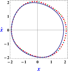
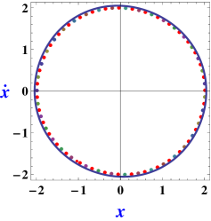
Figure 8: Comparison of limit cycles given by the approximate solution $\left(\text{\ref{RG Sol}}\right)$ using RGM (in dotted line) with the exact numerical limit cycle (in solid line) for $\left(a\right)$ $\varepsilon=0.5,\ k=F=0.5,$ $\sigma=0.1$ and $\left(b\right)\ \varepsilon=0.1,\ k=F=0.25,$ $\sigma=0.05$.

Next, for

$$\varepsilon=0.1,\ k=F=0.25,\ \sigma=0.05$$ (5.15)

we have

$$\rho=1.5971\times 10^{-2},\ 0.91599\text{ and }1.068\text{.}$$

As discussed in [1] for $k>0$ the largest value of $\rho$ always gives stable limit cycle. Therefore, we take the largest value $\rho=1.068$ so that

$$\Delta=3.99\times 10^{-2}>0\text{.}$$

Therefore, this choice of parameters given by $\left(\text{\ref{RFRL Parameter Val2}}\right)$ satisfy both the convergence criteria

$$\Delta>0\text{ and }\rho>\frac{1}{2}\text{.}$$

Thus, for this values of the parameters the limit cycle given by $\left(\text{\ref{RG Sol}}\right)$ is shown in Figure 8 by dotted line along with the numerical (exact) limit cycle in solid line for the Rayleigh equation $\left(\text{\ref{RFRL Eqn}}\right)$.

References

- [1] A. H. Nayfeh and D. T. Mook, Nonlinear Oscillations. John Wiley & Sons, 2008.
- [2] D. W. Jordan and P. Smith, Nonlinear Ordinary Differential Equations. Oxford University Press, 1999.
- [3] M. Lakshmanan and K. Murali, Chaos in Nonlinear Oscillators: Controlling and Synchronization. World scientific, 1996.
- [4] C. M. Bender and S. A. Orszag, Advanced Mathematical Methods for Scientists and Engineers I: Asymptotic Methods and Perturbation Theory. Springer Science & Business Media, 2013.
- [5] D. H. Bailey, R. Barrio, and J. M. Borwein, “High-precision computation: Mathematical physics and dynamics,” Applied Mathematics and Computation, vol. 218, no. 20, pp. 10 106–10 121, 2012.
- [6] D. P. Datta and S. Sen, “Excitation of flow instabilities due to nonlinear scale invariance,” Physics of Plasmas, vol. 21, no. 5, p. 052311, May 2014.
- [7] A. Palit and D. P. Datta, “Comparative study of homotopy analysis and renormalization group methods on rayleigh and van der pol equations,” Differential Equations and Dynamical Systems, vol. 24, no. 4, pp. 417–443, 2016.
- [8] D. P. Datta and S. Sarkar, “Duality structure, asymptotic analysis and emergent fractal sets,” Nonlinear Studies, vol. 25, no. 3, pp. 609–640, 2018.
- [9] D. P. Datta, S. Sarkar, and S. Raut, “Novel excitation of local fractional dynamics,” Nonlinear Studies, vol. 27, no. 4, pp. 935–956, 2020.
- [10] N. Goldenfeld, Lectures On Phase Transitions And The Renormalization Group. CRC Press, 2018.
- [11] S. Liao, Beyond Perturbation: Introduction to the Homotopy Analysis Method. CRC Press, 2003.
- [12] J. Cui, W. Zhang, Z. Liu, and J. Sun, “On the limit cycles, period-doubling, and quasi-periodic solutions of the forced van der pol-duffing oscillator,” Numerical Algorithms, vol. 78, no. 4, pp. 1217–1231, 2018.
- [13] Y. Li and L. Huang, “New results of periodic solutions for forced rayleigh-type equations,” Journal of Computational and Applied Mathematics, vol. 221, no. 1, pp. 98–105, 2008.
- [14] J. W. S. B. Rayleigh, The Theory of Sound. London, Macmillan and co, 1877.
- [15] Y. Xu and A. C. Luo, “Frequency-amplitude characteristics of periodic motions in a periodically forced van der pol oscillator,” The European Physical Journal Special Topics, vol. 228, no. 9, pp. 1839–1854, 2019.
- [16] A. K. Shukla, T. R. Ramamohan, and S. Srinivas, “A new analytical approach for limit cycles and quasi-periodic solutions of nonlinear oscillators: The example of the forced van der pol duffing oscillator,” Physica Scripta, vol. 89, no. 7, p. 075202, 2014.
- [17] L. Perko, Differential Equations and Dynamical Systems. Springer Science & Business Media, 2013.
- [18] L. Cveticanin, G. A. El-Latif, A. El-Naggar, and G. Ismail, “Periodic solution of the generalized rayleigh equation,” Journal of Sound and Vibration, vol. 318, no. 3, pp. 580–591, 2008.
- [19] J. H. He, “Some asymptotic methods for strongly nonlinear equations,” International Journal of Modern Physics B, vol. 20, no. 10, pp. 1141–1199, 2006.
- [20] C. S. Liu, “The renormalization method based on the taylor expansion and applications for asymptotic analysis,” Nonlinear Dynamics, vol. 88, no. 2, pp. 1099–1124, 2017.
- [21] A. C. Luo and S. Guo, “Analytical solutions of period-1 to period-2 motions in a periodically diffused brusselator,” Journal of Computational and Nonlinear Dynamics, vol. 13, no. 9, p. 090912, 2018.
- [22] A. C. Luo, Analytical Routes to Chaos in Nonlinear Engineering. John Wiley & Sons, 2014.
- [23] S. Raut and D. P. Datta, “Non-archimedean scale invariance and cantor sets,” Fractals, vol. 18, no. 01, pp. 111–118, 2010.
- [24] D. P. Datta, “Asymptotic linear-nonlinear duality, indeterminism and mathematical intelligence,” Chaos, Solitons & Fractals, 2021, Under Revision.
- [25] G. I. Barenblatt, Scaling, Self-similarity, and Intermediate asymptotics: Dimensional Analysis and Intermediate Asymptotics. Cambridge University Press, 1996.
- [26] L. Y. Chen, N. Goldenfeld, and Y. Oono, “Renormalization group and singular perturbations: Multiple scales, boundary layers, and reductive perturbation theory,” Physical Review E, vol. 54, no. 1, pp. 376–394, 1996.
- [27] R. L. DeVille, A. Harkin, M. Holzer, K. Josić, and T. J. Kaper, “Analysis of a renormalization group method and normal form theory for perturbed ordinary differential equations,” Physica D: Nonlinear Phenomena, vol. 237, no. 8, pp. 1029–1052, 2008.
- [28] A. Sarkar and J. Bhattacharjee, “Renormalization group as a probe for dynamical systems,” Journal of Physics: Conference Series, vol. 319, no. 1, p. 012017, 2011.
- [29] W. Szemplińska-Stupnicka and J. Rudowski, “Steady states in the twin-well potential oscillator: Computer simulations and approximate analytical studies,” Chaos: An Interdisciplinary Journal of Nonlinear Science, vol. 3, no. 3, pp. 375–385, 1993.
- [30] S. Katok, -adic Analysis Compared with Real. American Mathematical Society, 2007.