rSVDdpd: A Robust Scalable Video Surveillance Background Modelling Algorithm

Abstract

A basic algorithmic task in automated video surveillance is to separate background and foreground objects. Camera tampering, noisy videos, low frame rate, etc., pose difficulties in solving the problem. A general approach that classifies the tampered frames, and performs subsequent analysis on the remaining frames after discarding the tampered ones, results in loss of information. Several robust methods based on robust principal component analysis (PCA) have been introduced to solve this problem. To date, considerable effort has been expended to develop robust PCA via Principal Component Pursuit (PCP) methods with reduced computational cost and visually appealing foreground detection. However, the convex optimizations used in these algorithms do not scale well to real-world large datasets due to large matrix inversion steps. Also, an integral component of these foreground detection algorithms is singular value decomposition which is nonrobust. In this paper, we present a new video surveillance background modelling algorithm based on a new robust singular value decomposition technique rSVDdpd which takes care of both these issues. We also demonstrate the superiority of our proposed algorithm on a benchmark dataset and a new real-life video surveillance dataset in the presence of camera tampering. Software codes and additional illustrations are made available at the accompanying website rSVDdpd Homepage (https://subroy13.github.io/rsvddpd-home/)

Keywords Video Surveillance  $\cdot$ Background Modelling  $\cdot$ Object Tracking  $\cdot$ Robust SVD

1 Introduction

Automated surveillance from noisy videos is an extremely important problem with applications in different areas such as defence, security, research and monitoring, etc. In such video surveillance, the basic algorithmic task is to separate the background of a video from the foreground or moving objects, based on the input image frames from a surveillance video. The modelled background and foreground are then widely used in different image processing and computer vision applications. The most well-known and oldest applications were monitoring human activities in traffic surveillance systems. However, recently many other applications have been developed based on the same principle of background modelling such as detection of movements of animals and insects to study their behaviours, vision-based hand gesture recognition, autonomous vehicle pilot systems, content-based video coding, etc. Even though much work has been done towards solving this problem (see Garcia et al. (1) for details), various challenges such as the presence of noisy frames, low frame rate of the camera, change in illumination, multimodal backgrounds, presence of small moving objects, camera tampering, etc., still present major hindrances. Mantini and Shah (2) define tampering as a change in the view of a surveillance camera, which may occur naturally or manually through unexpected or unauthorized actions. Reflection or glare of sunlight onto the camera lens, change in the camera view from daylight mode to night vision mode, defocusing of the camera lens, are some of the natural occurrences of tampering without any human intervention. On the other hand, intentionally covering or obstructing the view of the camera, rotating the camera to point in different directions, etc. are examples of manual tampering with malicious intent. The goal associated with the analysis of such video surveillance data in presence of camera tampering is primarily to classify the video frames as tampered or non-tampered ones; then the non-tampered frames are used for solving different computer vision problems of interest. Several approaches (3; 4) have been developed to solve the above classification problem based on sophisticated image processing and deep learning techniques intended to detect the presence of such tampering. However, these techniques achieve good results only at the cost of an extensive amount of training data and computing power. Moreover, if the ultimate goal is to perform background modelling, discarding the tampered frames can result in loss of information, since if a frame is partially covered, the uncovered regions may still provide useful information including information about the unauthorized perpetrator. A robust methodology to extract the background and foreground should be able to make use of that information and provide valid and efficient inference under contaminated and noisy data.

Various methods for background modelling and foreground detection for video surveillance data have been developed in the past two decades. The different models can be classified into mathematical models (mean (5; 6), statistical (7; 8), fuzzy (9; 10), Dempster-Schafer concepts (11)), machine learning models (subspace learning (12; 13), neural networks (14) and deep learning methods (15; 16)), and signal processing methods (filter (17), sparse representation (18) and graph signal processing (19)). Some of them are unsupervised methods as subspace learning methods, supervised as deep learning methods (16) and semi-supervised as graph signal processing methods (19). The deep learning methods appear to offer the best performances; however, they require a large volume of labelled data and their performances decrease dramatically in the presence of unseen data. This is because these methods focus on improving the accuracy without modelling the underlying video data generation process in proper theoretical (or statistical) way. In contrast, unsupervised methods are backed by rich theoretical properties, require no labelled training data apriori and can be used in real-time applications. Among these, methods based on robust principal component analysis (PCA) have been shown to deliver state-of-the-art performances (20) compared to the traditional approaches of background modelling. These algorithms primarily rely on computing singular value decomposition (SVD) of some large matrices, which are highly susceptible to outliers. Usually, robust PCA algorithms circumvent this problem by computing truncated SVD multiple times and trimming any unreasonable solution to the factorization, due to which they become computationally expensive (21; 20; 1) and hence, of little practical use. Hence, while the deep learning methods are fast, scalable and parallelizable, they offer little theoretical justification and modelling of the background and foreground content. On the other hand, the unsupervised robust PCA based algorithms have a rich theoretical foundation, but they come at a high computational cost. In this paper, we propose a new background modelling and foreground estimation algorithm “rSVDdpd” based on a novel SVD methodology, which is unsupervised, theoretically justified, extremely robust and computationally efficient, thus correcting the deficiencies of each of the above approaches.

1.1 Related Work

Traditional approaches towards background modelling and foreground detection in video surveillance data followed various different approaches (22). Among classical techniques, the histogram based thresholding and running average methods (5; 6) were computationally simple and fast, but the performances of such algorithms were not appealing enough for practical use. Over the course of time, several sophisticated foreground detection methods were introduced based on statistical models of the background image or video. A review and comparison of several useful statistical background modelling algorithms have been compiled by Bouwmans et al. (7). All of these models consider a decomposition of the video surveillance data

$$\boldsymbol{X}=\boldsymbol{L}+\boldsymbol{S},$$ (1.1)

where $\boldsymbol{X}$ is the data matrix obtained by stacking the pixel values in all frames of a video as columns. This means, for a $p$-frame long video with each frame being $h$ pixels long and $w$ pixels wide, the $\boldsymbol{X}$ matrix becomes of dimension $hw\times p$. The component $\boldsymbol{L}$ in Eq. (1.1) corresponds to the background content of the video, which is assumed to be generated from some statistical model. For instance, MOG (8; 23; 24) and TensorMOG (25) algorithms have been developed on the assumption that each column of $\boldsymbol{L}$ follows a mixture of Gaussian distribution. On the other hand, there exists another class of statistical background modelling algorithms derived from Principal Component Analysis (PCA) which models the matrix $\boldsymbol{L}$ as low rank. For instance, if the camera is static and is able to capture moderate to high resolution video feed, then it is expected that the background pixels from one frame to another frame will only differ in illumination changes. In this particular case, each column in the $\boldsymbol{L}$ matrix is expected to be proportional to each other, i.e., the matrix $\boldsymbol{L}$ is expected to be of rank one only. In general, since the subsequent frames in a video are correlated, a suitable low rank approximation $\boldsymbol{L}$ should be able to extract the non-moving part of the video, i.e., the background objects, while the difference ($\boldsymbol{X}-\boldsymbol{L}$) should be able to extract the sparse and noisy part, namely the moving foreground objects. While the classical SVD by itself can obtain such a decomposition of $\boldsymbol{X}$ and is computationally extremely fast, it cannot be directly used for foreground detection and background modelling. As noted by several authors (26; 27; 28), the SVD by itself is not a robust procedure and is prone to the different kinds of outliers such as shadows, illumination changes, camera tampering, jittering etc., which are common in real-life video surveillance data. Thus, the recent background modelling algorithms focus on obtaining a robust estimate of $\boldsymbol{L}$ through a robust PCA formulation. Such PCA based algorithms (12; 29) have received considerable attention over the last decade as they have been found to be better than MOG algorithms for several benchmark datasets (20) and also have broad applicability (30). These algorithms minimize some objective function with respect to the eigenvalues and eigenvectors of $\boldsymbol{L}$, and the minimization is generally performed by a gradient descent algorithm on the Stiefel manifold (the Riemannian manifold of all orthogonal matrices of a fixed dimension) which is computationally extremely costly. Thus, although these methods produce superior results, they cannot be implemented in practice for real-time foreground detection of video surveillance data.

Based on the decomposition (1.1), the ideal problem to solve for foreground detection would have been

$$\min_{\boldsymbol{L},\boldsymbol{S}}\text{rank}(\boldsymbol{L})+\lambda\|\boldsymbol{S}\|_{0}$$ (1.2)

where $\lambda>0$ is an arbitrary balance parameter. However, performing this minimization is NP-hard, hence a reasonable approximate solution would be to consider

$$\min_{\boldsymbol{L},\boldsymbol{S}}\|\boldsymbol{L}\|_{\ast}+\lambda\|\boldsymbol{S}\|_{1}$$ (1.3)

where $\|\boldsymbol{L}\|_{\ast}$ denotes the nuclear norm (i.e., the sum of singular values) of $\boldsymbol{L}$. Candes et al. (21) define this problem as “Principal Component Pursuit” (PCP) and under the assumption that $\boldsymbol{L}$ is exactly low rank and $\boldsymbol{S}$ is exactly sparse, they are able to show that the solution of the approximate problem (1.3) perfectly recovers a solution of the ideal problem (1.2). Since this method, too, was computationally costly, numerous algorithms have been built to solve the Principal Component Pursuit problem as in Eq. (1.3) with less computational cost. Some optimization techniques like Augmented Lagrangian method (31), Gradient descent method (32), etc. have proven useful in this regard. Xu et al. (33) considered another variant of the ideal problem (1.2) called Outlier Pursuit (OP)

$$\min_{\boldsymbol{L},\boldsymbol{S}}\|\boldsymbol{L}\|_{\ast}+\lambda\|\boldsymbol{S}\|_{1,2}$$ (1.4)

where $\|\boldsymbol{S}\|_{1,2}$ is the sum of the $L_{2}$ norms of the columns of $\boldsymbol{S}$. One limitation of PCP and OP is that they assume the decomposition of the data $\boldsymbol{X}$ into the low rank matrix and the sparse matrix to be exact, but real life videos hardly satisfy that due to quantization of pixel values, measurement errors, shadows, artifacts, slowly moving backgrounds, etc. Therefore, a more realistic decomposition of the video surveillance data $\boldsymbol{X}$ is to consider

$$\boldsymbol{X}=\boldsymbol{L}+\boldsymbol{S}+\boldsymbol{N}$$ (1.5)

where $\boldsymbol{N}$ is a small perturbation matrix with independent elements, which is neither low rank nor sparse. Babacan et al. (34) apply a Bayesian modelling to the decomposition (1.5) and use Gibbs sampling to obtain posterior estimates of the low rank matrix $\boldsymbol{L}$ through sampling in the Stiefel manifold. In contrast, Liu et al. (35) used the Augmented Lagrangian method repeatedly to solve the problem

$$\min_{\boldsymbol{L},\boldsymbol{S}}\|\boldsymbol{L}\|_{\ast}+\beta\|\boldsymbol{S}\|_{0}+\lambda\|\boldsymbol{X}-\boldsymbol{L}-\boldsymbol{S}\|_{1}$$ (1.6)

where both $\lambda,\beta>0$ are penalty parameters that can be tuned.

1.2 Issues with existing works

Despite being extremely powerful, the robust PCA algorithms by themselves have several bottlenecks which limit their practical use. Various modifications of these algorithms have been proposed in the last decade including incremental algorithms (36; 37; 38) to identify foreground content as soon as new video frames are recorded, spatio-temporal algorithms (39; 40) which enable foreground detection to be motion aware, and algorithmic improvements (41; 42) to address scalability issues so that these algorithms can be used to estimate the background content in a large scale high-resolution video surveillance data within a reasonable time. There are two primary bottlenecks in reducing the computational complexity of these algorithms. One, these algorithms rely on the convex optimization problems as in Eq. (1.3) or (1.4) which present significant challenges in optimization in a high dimensional setting (43). Two, these algorithms use numerous truncated SVD, matrix multiplication and matrix inversion steps which have currently a computational complexity of $O(n^{2.37188})$ (44) for $n\times n$ matrices, and the order can grow rapidly and significantly for large values of $n$ in high dimensional matrices. To address both of these issues, we propose a novel algorithm to compute robust estimates of the singular values and vectors themselves, without requiring the formulation of a convex optimization problem as PCP, but rather a statistical robust regression problem. We also present an iterative algorithm based on the alternating regression trick, which circumvents the aforementioned computationally intensive steps and reduces the computational complexity to only $O(n^{2})$ in each iteration for an $n\times n$ matrix. Also, the iteration steps of the proposed algorithm are highly parallelizable, hence the algorithm can scale efficiently to arbitrarily high dimensional video surveillance data, within a reasonable amount of time, provided necessary memory requirements.

For example, as presented in Candes et al. (21), it takes about $13$ seconds per frame for the exact PCP method to converge for a $176\times 144$ low-resolution grayscale video, and clearly, this high computational complexity hinders its practical use despite having good performance for foreground extraction. In comparison, GRASTA algorithm (37) which does not take the robust PCA approach takes only $0.13$ seconds per frame to extract the foreground content of a video of the same resolution, but its performance accuracy does not match that of the robust PCA via the PCP approach (20). On the other hand, our proposed algorithm takes only $0.182$ seconds per frame to separate the background and foreground of a video of the same dimensionality and achieves the same level of accuracy as the exact PCP method.

1.3 Our contributions

In this paper, we aim to provide a novel background modelling and foreground extraction algorithm “rSVDdpd” via an alternative robust singular value decomposition methodology based on the popular density power divergence. The minimum density power divergence introduced by Basu et al. (45) has been proven to be robust and efficient in estimation in several contexts (46; 47). We leverage its robustness properties by directly applying it to the video surveillance background modelling problem, where the noisy and the sparse content can be viewed as outliers present in the data. As an illustration, we consider the “freeway” video sequence from UCSD Background Subtraction Dataset (48) consisting of $44$ frames of grayscale images of dimension $316\times 236$. It depicts a highway in the background with moving cars as foreground objects having different shades of gray. One can use the usual singular value decomposition (SVD) to extract such background and foreground content, but that usually becomes highly susceptible to noise present in the video surveillance data. Here, we add salt-and-pepper noise to only a few of the consecutive frames of the video as mild tampering, which ideally should affect only the tampered frames but not to the entire video. As shown in Figure 1, the usual SVD based background model works poorly even in non-tampered frames. In contrast, the proposed robust algorithm rSVDdpd is able to extract the foreground and background content very efficiently, by removing noisy artifacts such as moving shadows, illumination change, etc. Also, rSVDdpd solves a non-convex optimization problem by an alternating fixed point iteration method. Each step of the iteration is computationally extremely simple to perform, requiring only scalar inner product computations, which are highly parallelizable making it suitable for very high dimensional or high resolution video surveillance applications.

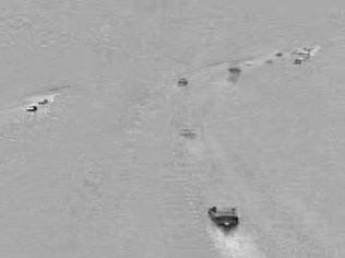
(a)

(b)

(c)

Figure 1: The true images, background and foreground images estimated by usual SVD and the proposed rSVDdpd method (from left to right in a row), corresponding to frame 5 (a), 18 (b) and 42 (c) of the “freeway” video sequence. Enlarged better quality images are available online at https://subroy13.github.io/rsvddpd-home/.

In summary, we aim to make the following contributions in this paper.

• Propose a fast, robust and scalable alternative to the video surveillance background modelling problem through robust singular value decomposition.

• We compare the proposed rSVDdpd algorithm with several existing background modelling algorithms on the Background Model Challenge Benchmark dataset to show its effectiveness.

• We also demonstrate how rSVDdpd can obtain reliable background and foreground estimates in the presence of camera tampering by showing its performance on a novel real-life “University of Houston Camera Tampering Dataset” (UHCTD).

• In this paper, we also discuss various desirable theoretical properties the rSVDdpd estimate enjoys.

The rest of the paper is organized as follows. In Section 2, we develop our background modelling algorithm from a regression based and a penalty based approach. Following this development, we present the convergence results and some basic mathematical properties of the proposed rSVDdpd estimator in Section 2.4. Section 3 contains the experimental results regarding the performance comparison of different background modelling algorithms on the Background Model Challenge Benchmark dataset. Finally, in Section 3.3, we also make a similar comparison on a novel real-life dataset UHCTD to demonstrate the superiority of our method in the presence of camera tampering, and some concluding remarks are presented in Section 4.

2 Proposed rSVDdpd Method

Instead of the decomposition as in Eq. (1.5), we combine $\boldsymbol{S}$ and $\boldsymbol{N}$ into a single error matrix $\boldsymbol{E}$, whose elements are small independent noise component except certain spikes due to the sparse component $\boldsymbol{S}$. Let the video surveillance data matrix $\boldsymbol{X}$ be of dimension $n\times p$ ($n$ and $p$ may be different) and the low rank component $\boldsymbol{L}$ is of rank $r$, where $r$ is much lower than $n$ or $p$. Then, the decomposition of $\boldsymbol{X}$ can be expressed in terms of the singular values and vectors of $\boldsymbol{L}$, namely

$$\boldsymbol{X}=\sum_{k=1}^{r}\lambda_{k}\boldsymbol{u}_{k}\boldsymbol{v}_{k}^{\mathsf{T}}+\boldsymbol{E},$$ (2.1)

where $\boldsymbol{u}_{k}$ is a vector of length $n$ and $\boldsymbol{v}_{k}$ is a vector of length $p$ for $k=1,2,\dots r$, and $\boldsymbol{E}$ is a $n\times p$ matrix. The entries of the error matrix $\boldsymbol{E}$, i.e., $e_{ij}$s are generally expected to be smaller in magnitude than the corresponding entry of the data matrix $\boldsymbol{X}$, except for some outlying values corresponding to the pixels of the foreground object in different frames. The left singular vectors $\{\boldsymbol{u}_{k}\}_{k=1,2,\dots r}$’s and the right singular vectors $\{\boldsymbol{v}_{k}\}_{k=1,2,\dots r}$’s also satisfy the orthonormality constraints, i.e.,

$$\boldsymbol{u}_{k}^{\mathsf{T}}\boldsymbol{u}_{l}=\begin{cases}1&\text{ if }k=l\\ 0&\text{ if }k\neq l\end{cases},\quad\boldsymbol{v}_{k}^{\mathsf{T}}\boldsymbol{v}_{l} =\begin{cases}1&\text{ if }k=l\\ 0&\text{ if }k\neq l\end{cases}$$

$$\qquad k,l=1,2,\dots r,$$

and the singular values $\lambda_{k}$ satisfy the nonnegativity constraints. As in (49), the above description can also be reformulated into a matrix factorization as

$$\boldsymbol{X}=\sum_{k=1}^{r}\boldsymbol{a}_{k}\boldsymbol{b}_{k}^{\mathsf{T}}+E,$$ (2.2)

where $\boldsymbol{a}_{k}$s and $\boldsymbol{b}_{k}$s are still orthogonal sets of vectors for $k=1,2,\dots r$, but not necessarily normalized. Once the estimates of $\boldsymbol{a}_{k}$s and $\boldsymbol{b}_{k}$s are known, they can be normalized to obtain the $\boldsymbol{u}_{k}$s and $\boldsymbol{v}_{k}$s and the singular values are then given by $\lambda_{k}=\|\boldsymbol{a}_{k}\|\|\boldsymbol{b}_{k}\|$ for each $k=1,\ldots,r$, where $\|\cdot\|$ denotes the usual Euclidean ($L_{2}$) norm.

For the computation of the left and right singular vectors from Eq. (2.2), one can proceed sequentially focusing only on a rank one approximation as follows. First, consider the approximation $\boldsymbol{X}\approx\boldsymbol{a}_{1}\boldsymbol{b}_{1}^{\mathsf{T}}$. Once we have estimates for $\widehat{\boldsymbol{a}}_{1}$ and $\widehat{\boldsymbol{b}}_{1}$, we can obtain $\widehat{\lambda}_{1}=\|\widehat{\boldsymbol{a}}_{1}\|\|\widehat{\boldsymbol{b}}_{1}\|$, and normalize $\widehat{\boldsymbol{a}}_{1}$ and $\widehat{\boldsymbol{b}}_{1}$ as required. Next, we compute the residual matrix $\boldsymbol{X}-\widehat{\boldsymbol{a}}_{1}\widehat{\boldsymbol{b}}_{1}^{\mathsf{T}}$, and the rank one approximation algorithm can be used again on this residual matrix, to obtain the second singular value and the corresponding vectors. Proceeding similarly, one can compute all $r$ singular values and singular vectors of the given data matrix $\boldsymbol{X}$. Therefore, for ease of explanation, we will describe the algorithm only for obtaining the vectors $\boldsymbol{a}$ and $\boldsymbol{b}$ yielding the best rank-one approximation of the data matrix $\boldsymbol{X}$ as

$$\boldsymbol{X}\approx\boldsymbol{a}\boldsymbol{b}^{\mathsf{T}}.$$ (2.3)

Accordingly, in the following, we shall use $a_{i}$ for $i=1,2,\dots n$, to denote the elements of the vector $\boldsymbol{a}$ and similarly, $b_{j}$ for $j=1,2,\dots p$, to denote the elements of the vector $\boldsymbol{b}$. The elements of the $\boldsymbol{X}$ matrix are denoted by $x_{ij}$.

2.1 The Regression based approach

We consider the idea of transforming the SVD estimation problem into a regression problem, following (49). For this purpose, let us first fix the index $j$ (i.e., the column index), and consider the setup

$$X_{ij}=a_{i}b_{j}+e_{ij},\qquad i=1,2,\dots n,$$ (2.4)

which is a simple linear regression problem without any intercept. Here, $x_{ij}$s are observed response variables and $e_{ij}$s are random error components. Therefore, for any given value of $\boldsymbol{a}$, we can treat $a_{i}$s as covariate values and estimate the $b_{j}$s as regression slopes, and as we vary the column index $j=1,2,\dots p$, we are posed with $p$ such linear regression problems, jointly yielding an estimate of $\boldsymbol{b}=(b_{1},\ldots,b_{p})$. Next, given these estimated values of $b_{j}$s, we treat them as covariates in Eq. (2.4) and estimate the $a_{i}$s as the unknown regression parameters for each $i=1,\ldots,n$. Repeating these two steps sequentially until convergence, we get the final desired estimates of $\boldsymbol{a}$ and $\boldsymbol{b}$ from which the desired singular value and vectors can be obtained as discussed previously.

Now, for estimating the regression coefficients ($b_{j}$ or $a_{i}$) in each iteration of the aforementioned alternating regression approach, we propose to use the robust and efficient minimum Density Power Divergence (DPD) estimation procedure. The minimum DPD estimator (MDPDE) was initially developed for independent and identically distributed data in (45), and later extended to the more general independent non-homogeneous set-up in (46). It considers a general form of DPD-based loss function involving

$$V_{i}(y_{i};\boldsymbol{\theta})=\left[\int f_{i}(y;\boldsymbol{\theta})^{1+\alpha}dy-\left(1+\frac{1}{\alpha}\right)f_{i}(y_{i};\boldsymbol{\theta})^{\alpha}\right],$$ (2.5)

where $\alpha>0$ is the robustness tuning parameter, and the distribution of the $i$-th sample observation $y_{i}$ is modeled using a parametric family of distributions $\mathcal{F}_{i}=\{f_{i}(y;\boldsymbol{\theta}):\boldsymbol{\theta}\in\boldsymbol{\Theta}\}$ for each $i$. As a particular case, the MDPDE under the linear regression model with normally distributed errors are also discussed in (46), which can be used in the present context. For our purpose, as in the classical setup of the robust statistics, we can model the error components $e_{ij}$s in Eq. (2.4) to be independent and normally distributed with mean zero and variance $\sigma^{2}$, except for some outliers due to the spikes that are present in the $\boldsymbol{E}$ matrix. Therefore, the MDPDE objective function for estimating the unknown parameters $a_{i}$ or $b_{j}$ and $\sigma^{2}$ from Eq. (2.4), turns out to be

$$H_{n,p}(\boldsymbol{a},\boldsymbol{b},\sigma^{2})=\dfrac{1}{np}\sum_{i=1}^{n}\sum_{j=1}^{p}V(x_{ij};a_{i},b_{j},\sigma^{2}),$$ (2.6)

where

$$V(y;c,d,\sigma^{2})=(2\pi)^{-\alpha/2}\sigma^{-\alpha}\left[(1+\alpha)^{-1/2}\right.\\ \left.-\frac{(1+\alpha)}{\alpha}\exp\left\{-\alpha\frac{(y-cd)^{2}}{2\sigma^{2}}\right\}\right],$$ (2.7)

is a simplification of Eq. (2.5) with $f_{i}(y,\boldsymbol{\theta})$ as the density of a normal distribution with mean $cd$ and variance $\sigma^{2}$. The MDPDE of the parameter $\boldsymbol{\theta}=(\boldsymbol{a},\boldsymbol{b},\sigma^{2})$ is then obtained by minimizing this objective function in Eq. (2.6) with respect to each of the components of the triplet. So, instead of estimating the elements of the scaled singular vectors $\boldsymbol{a}$ and $\boldsymbol{b}$, i.e., $a_{i}$s and $b_{j}$s in the alternating regression models, we can indeed minimize this MDPDE objective function iteratively over either of the parameters ($a_{i}$, $b_{j}$ or $\sigma^{2}$) given the most recent estimates of the other parameters. By standard differentiation, as in (46), the corresponding estimating equations turn out to be

$$\sum_{j=1}^{p}b_{j}(x_{ij}-a_{i}b_{j})e^{-\alpha\frac{(x_{ij}-a_{i}b_{j})^{2}}{2\sigma^{2}}} =0,\ i=1,\ldots n,$$ (2.8)

$$\sum_{i=1}^{n}a_{i}(x_{ij}-a_{i}b_{j})e^{-\alpha\frac{(x_{ij}-a_{i}b_{j})^{2}}{2\sigma^{2}}} =0,\ j=1,\ldots p,$$ (2.9)

$$\sum_{i=1}^{n}\sum_{j=1}^{p}\left[1-\frac{(x_{ij}-a_{i}b_{j})^{2}}{\sigma^{2}}\right]e^{-\alpha\frac{(x_{ij}-a_{i}b_{j})^{2}}{2\sigma^{2}}} =\frac{\alpha}{(1+\alpha)^{3/2}}.$$ (2.10)

From another viewpoint, the mentioned proposal yields a robust generalization of the ususal SVD estimators for $\alpha>0$. To see this, denoting $w_{ij}=e^{-\alpha\frac{(x_{ij}-a_{i}b_{j})^{2}}{2\sigma^{2}}}$, it follows that the estimating equations in Eq. (2.8)-(2.10) can be rearranged into the form

$$\begin{split}a_{i}&=\dfrac{\sum_{j}b_{j}x_{ij}w_{ij}}{\sum_{j}b_{j}^{2}w_{ij}},\ i=1,\ldots n;\\ b_{j}&=\dfrac{\sum_{i}a_{i}x_{ij}w_{ij}}{\sum_{i}a_{i}^{2}w_{ij}},\ j=1,\ldots p;\\ \sigma^{2}&=\dfrac{\sum_{i}\sum_{j}(x_{ij}-a_{i}b_{j})^{2}w_{ij}}{\sum_{i}\sum_{j}w_{ij}-\frac{\alpha}{(1+\alpha)^{3/2}}}.\end{split}$$ (2.11)

In the first estimating equation of Eq. (2.11), as $x_{ij}\approx a_{i}b_{j}$, i.e., $x_{ij}/b_{j}\approx a_{i}$, the equation considers the weighted mean of $x_{ij}/b_{j}$ with weights $b_{j}^{2}w_{ij}$. Similar normalization is also present in the second equation. In the third equation, we see that $\sigma^{2}$ is approximately a normalized version of the squared residuals $(x_{ij}-a_{i}b_{j})^{2}$ except for a term subtracted from the denominator to make the corresponding estimating equation unbiased. Thus, each of the parameters are estimated as a weighted average of different crude estimates based on the elements of the data matrix $\boldsymbol{X}$ and the most recent values of the other parameters. Also, for any $\alpha>0$, $w_{ij}=e^{-\alpha\frac{(x_{ij}-a_{i}b_{j})^{2}}{2\sigma^{2}}}$ is a decreasing function of the magnitude of the residuals, i.e., of $|x_{ij}-a_{i}b_{j}|$. This decreasing nature is crucial to make the overall estimates robust since a large deviation from the model having large $|x_{ij}-a_{i}b_{j}|$ would yield smaller weights, and hence those outlying values would have little effect on the estimating equations given in Eq. (2.11).

The particular form of these weights $w_{ij}$ in Eq. (2.11) appears due to the assumption of normality of the errors $e_{ij}$. In a more general version with appropriately modified weight function, one can consider the estimating equations

$$a_{i} =\dfrac{\sum_{j}b_{j}x_{ij}\psi(|x_{ij}-a_{i}b_{j}|)}{\sum_{j}b_{j}^{2}\psi(|x_{ij}-a_{i}b_{j}|)},\qquad i=1,\ldots n,$$ (2.12)

$$b_{j} =\dfrac{\sum_{i}a_{i}x_{ij}\psi(|x_{ij}-a_{i}b_{j}|)}{\sum_{i}a_{i}^{2}\psi(|x_{ij}-a_{i}b_{j}|)},\qquad j=1,\ldots p,$$ (2.13)

$$\sigma^{2} =\dfrac{\sum_{i}\sum_{j}(x_{ij}-a_{i}b_{j})^{2}\psi(|x_{ij}-a_{i}b_{j}|)}{\sum_{i}\sum_{j}\psi(|x_{ij}-a_{i}b_{j}|)-S_{\psi}}.$$ (2.14)

where $\psi(\cdot)$ is a suitably smooth and decreasing function of its argument, and $S_{\psi}$ is a suitably chosen quantity to make the estimating equation corresponding to $\sigma^{2}$ unbiased.

2.2 Orthogonalization of Singular Vectors

In the mathematical framework developed in Section 2.1, there is no component in the regression formulation that ensures orthogonality of the singular vectors. It is natural to extend the objective function $H_{n,p}(\boldsymbol{a},\boldsymbol{b},\sigma^{2})$ of Eq. (2.6) using a penalty function to achieve the orthogonality requirements. One such penalty function could be the sum of the squared inner products (dot-products) of the current singular vector with all preceding singular vectors.

To formulate this penalized approach, let us assume, $\boldsymbol{a}_{1},\boldsymbol{a}_{2},\dots,\boldsymbol{a}_{k}$ be the $k$ non-normalized left singular vectors and $\boldsymbol{b}_{1},\boldsymbol{b}_{2},\dots,\boldsymbol{b}_{k}$ be the $k$ non-normalized right singular vectors of the data matrix $\boldsymbol{X}$, leading to the singular values $\lambda_{l}=\|\boldsymbol{a}_{l}\|\|\boldsymbol{b}_{l}\|$ for $l=1,\ldots,k$. This amounts to assuming that we already have the rank $k$ approximation of the data matrix as

$$\boldsymbol{X}\approx\sum_{r=1}^{k}\boldsymbol{a}_{r}\boldsymbol{b}_{r}^{\mathsf{T}}.$$

With these already estimated (non-normalized) singular vectors $\boldsymbol{a}_{1},\dots\boldsymbol{a}_{k},\boldsymbol{b}_{1},\dots\boldsymbol{b}_{k}$, the task of obtaining the next orthogonal (non-normalized) singular vectors $\boldsymbol{a}_{(k+1)}$ and $\boldsymbol{b}_{(k+1)}$ (assume $k\leq\text{rank}(\boldsymbol{X})-1$) becomes the same as finding a rank one decomposition like Eq. (2.3) of the transformed data matrix $\boldsymbol{X}^{\prime}=\left(\boldsymbol{X}-\sum_{r=1}^{k}\boldsymbol{a}_{r}\boldsymbol{b}_{r}^{\mathsf{T}}\right)$ subject to the conditions

$$\boldsymbol{a}^{\mathsf{T}}\boldsymbol{a}_{r}=\boldsymbol{b}^{\mathsf{T}}\boldsymbol{b}_{r}=0,\qquad r=1,2,\dots k.$$

Thus, we can again use the alternating regression approach to estimate the parameters $\boldsymbol{a},\boldsymbol{b},\sigma^{2}$ iteratively and consider the penalized MDPDE objective function with Lagrangian parameter $\xi$ as

$$\widetilde{H}_{k;n,p}(\boldsymbol{a},\boldsymbol{b},\sigma^{2})=\dfrac{1}{np}\sum_{i=1}^{n}\sum_{j=1}^{p}V\left(x^{\prime}_{ij};a_{i},b_{j},\sigma^{2}\right)\\ +\dfrac{\xi}{k}\left[\sum_{r=1}^{k}\dfrac{(\boldsymbol{a}^{\mathsf{T}}\boldsymbol{a}_{r})^{2}}{\|\boldsymbol{a}_{r}\|^{2}}+\sum_{r=1}^{k}\dfrac{(\boldsymbol{b}^{\mathsf{T}}\boldsymbol{b}_{r})^{2}}{\|\boldsymbol{b}_{r}\|^{2}}\right],\\ k=1,2,\dots\text{rank}(\boldsymbol{X}-1),$$ (2.15)

where $x^{\prime}_{ij}$ is the $(i,j)$-th element of $\boldsymbol{X}^{\prime}$. Notice that the normalization factors $\|\boldsymbol{a}_{r}\|^{2}$ and $\|\boldsymbol{b}_{r}\|^{2}$ have been used in Eq. (2.15) to make sure that each penalty term is of similar magnitude.

Again, differentiating the objective function in Eq. (2.15) with respect to the individual parameters and setting them equal to 0, yields the estimating equations for the parameters $\boldsymbol{a},\boldsymbol{b},\sigma^{2}$. A reorganization of the estimating equations lead to a fixed point iteration formula similar to Eq. (2.11) as given by

$$\begin{split}a_{i}&=\left(\sum_{j=1}^{p}b_{j}^{2}w_{ij}\right)^{-1}\left[\sum_{j=1}^{p}b_{j}x^{\prime}_{ij}w_{ij}+C_{\xi}\sum_{r=1}^{k}(\boldsymbol{a}_{r}^{\mathsf{T}}\boldsymbol{a})(\boldsymbol{a}_{r})_{i}\right],\\ &\qquad\qquad i=1,\dots n,\\ b_{j}&=\left(\sum_{i=1}^{n}a_{i}^{2}w_{ij}\right)^{-1}\left[\sum_{i=1}^{n}a_{i}x^{\prime}_{ij}w_{ij}+C_{\xi}\sum_{r=1}^{k}(\boldsymbol{b}_{r}^{\mathsf{T}}\boldsymbol{b})(\boldsymbol{b}_{r})_{j}\right],\\ &\qquad\qquad j=1,\dots p,\\ &\qquad\qquad k=1,2,\dots\text{rank}(\boldsymbol{X})-1,\end{split}$$ (2.16)

where $w_{ij}=e^{-\alpha\frac{(x^{\prime}_{ij}-a_{i}b_{j})^{2}}{2\sigma^{2}}}$, and $C_{\xi}=\frac{np(2\pi)^{(\alpha/2)}\sigma^{\alpha}\xi}{k(1+\alpha)}$. Since, the penalty term is not a function of $\sigma^{2}$, the estimating equation corresponding to $\sigma^{2}$ remains same as in Eq. (2.11).

Unfortunately, the convergence of the algorithm with estimating equations Eq. (2.16) is highly sensitive to the choice of Lagrangian penalty parameter $\xi$. Often, the choice of $\xi$ can be obtained through a cross validation approach as in (50). However, this adds another level of complexity to the algorithm making it computationally expensive. Since, our aim is to obtain a fast and accurate algorithm for the decomposition (1.5) for video surveillance data, we circumvent the problem using an orthogonalization trick similar to Gram Schimdt orthogonalization process (51). In particular, between alternatively using Eq. (2.8)-(2.10), the estimates $\boldsymbol{a}$ and $\boldsymbol{b}$ are updated as

$$\boldsymbol{a}\leftarrow\boldsymbol{a}-\sum_{r=1}^{k}{\boldsymbol{a}}^{\mathsf{T}}\boldsymbol{a}_{r},\ \boldsymbol{b}\leftarrow\boldsymbol{b}-\sum_{r=1}^{k}{\boldsymbol{b}}^{\mathsf{T}}\boldsymbol{b}_{r},\$$ (2.17)

where the symbol $\leftarrow$ denotes the assignment operator, i.e., the value of left hand side of Eq. (2.17) is updated with the value of the right hand side. Note that, such an orthogonalization step need not be performed for the first singular value, but is performed only from the estimation of the subsequent singular values. Including the singular values $\lambda$ and restricting the vectors $\boldsymbol{a}$ and $\boldsymbol{b}$ to have unit $L_{2}$-norm, we ultimately consider the estimation of the parameter $\boldsymbol{\theta}=(\lambda,\boldsymbol{a},\boldsymbol{b},\sigma^{2})$. The final algorithm has been outlined below in Figure 2.

0:  Video frames $\boldsymbol{V}$ of dimension $h\times w\times p$, $0<\alpha<1$, background rank $r\geq 0$.

  Initialize matrix $\boldsymbol{X}_{hw\times p}$.

  for $i=1$ to $p$ do

     $\boldsymbol{X}[,i]\leftarrow\text{vec}(\boldsymbol{V}[,,i])$

  end for

  for $k=1$ to $r$ do

     Let $\boldsymbol{a}_{1}^{\ast},\boldsymbol{a}_{2}^{\ast},\dots,\boldsymbol{a}_{k}^{\ast}$ and $\boldsymbol{b}_{1}^{\ast},\boldsymbol{b}_{2}^{\ast},\dots,\boldsymbol{b}_{k}^{\ast}$ are $k$ estimated singular vectors already obtained.

     Initialize $\lambda_{k+1}^{(0)},\boldsymbol{a}_{k+1}^{(0)},\boldsymbol{b}_{k+1}^{(0)}$ as first singular value and left and right singular vectors of $\boldsymbol{X}$.

     $t\leftarrow 0$.

     repeat

        $\boldsymbol{c}\leftarrow\boldsymbol{a}_{k+1}^{(t)}$

        $w_{ij}\leftarrow\exp\left(-\dfrac{(x_{ij}-c_{i}b_{(k+1)j}^{(t)})^{2}}{2(\sigma^{2})^{(t)}}\right)$

        for $i=1,2,\dots hw$ do

           $c_{i}\leftarrow\left(\dfrac{\sum_{j}w_{ij}^{\alpha}x_{ij}(b_{(k+1)j}^{(t)})}{\sum_{j}w_{ij}^{\alpha}(b_{(k+1)j}^{(t)})^{2}}\right)$

        end for

        $\boldsymbol{c}\leftarrow\boldsymbol{c}-\sum_{r=1}^{k}\boldsymbol{c}^{\top}\boldsymbol{a}_{r}$.

        $\lambda_{(k+1)}^{(t+1)}\leftarrow\|\boldsymbol{c}\|$.

        $\boldsymbol{a}_{k+1}^{(t+1)}\leftarrow\boldsymbol{c}/\lambda_{(k+1)}^{(t+1)}$

        $\boldsymbol{d}\leftarrow\boldsymbol{b}_{k+1}^{(t)}$

        $w_{ij}\leftarrow\exp\left(-\dfrac{(x_{ij}-a_{(k+1)i}^{(t+1)}d_{j})^{2}}{2(\sigma^{2})^{(t)}}\right)$

        for $j=1,2,\dots p$ do

           $d_{j}\leftarrow\left(\dfrac{\sum_{i}w_{ij}^{\alpha}x_{ij}(a_{(k+1)i}^{(t+1)})}{\sum_{i}w_{ij}^{\alpha}(a_{(k+1)i}^{(t+1)})^{2}}\right)$

        end for

        $\boldsymbol{d}\leftarrow\boldsymbol{d}-\sum_{r=1}^{k}\boldsymbol{d}^{\top}\boldsymbol{b}_{r}$.

        $\lambda_{(k+1)}^{(t+1)}\leftarrow\|\boldsymbol{d}\|$.

        $\boldsymbol{b}_{k+1}^{(t+1)}\leftarrow\boldsymbol{d}/\lambda_{(k+1)}^{(t+1)}$.

        $e_{ij}\leftarrow x_{ij}-\lambda_{(k+1)}^{(t+1)}a_{(k+1)i}^{(t+1)}b_{(k+1)j}^{(t+1)}$

        $w_{ij}\leftarrow\exp(e_{ij})$

        $(\sigma^{2})^{(t+1)}\leftarrow\dfrac{\sum_{i}\sum_{j}w_{ij}^{\alpha}e_{ij}^{2}}{\sum_{i}\sum_{j}w_{ij}^{\alpha}-(\alpha/(1+\alpha)^{3/2})}$

        $t\leftarrow(t+1)$

     until convergence

     $X\leftarrow X-\lambda_{(k+1)}^{(t+1)}\boldsymbol{a}_{(k+1)}^{(t+1)}(\boldsymbol{b}_{(k+1)}^{(t+1)})^{\top}$

  end for

  Output: Background = $\sum_{k=1}^{r}\widehat{\lambda}_{k}^{(t+1)}\widehat{a}_{k}^{(t+1)}\left(\widehat{b}_{k}^{(t+1)}\right)^{\top}$ where each column is converted into an image of dimension $h\times w$.

Figure 2: rSVDdpd Background Modelling Algorithm

2.3 Choice of hyperparameters

There are two hyperparameters to the rSVDdpd algorithm: the robustness parameter $\alpha\in[0,1]$ and the rank of the matrix $\boldsymbol{L}$ representing background content. The robustness parameter $\alpha$ in the objective function (2.6) provides a bridge between robustness and efficiency of estimation. Through extensive simulation studies, we have seen that higher values of the robustness parameter $\alpha$ tend to produce background estimates with smaller bias, under any kind of contamination. On the other side of the coin, the estimated pixel values of the background content exhibit higher variance with an increase in $\alpha$. To determine the optimal choice of $\alpha$, we consider a conditional MSE criterion as in (52). Some elementary calculation yields that the optimal choice of the robustness parameter is the minimizer of the criterion

$$(n+p)(\widehat{\sigma}^{(\alpha)})^{2}\left(1+\dfrac{\alpha^{2}}{1+2\alpha}\right)^{3/2}\\ +\dfrac{1}{r}\sum_{k=1}^{r}\|\widehat{\lambda}_{k}^{(\alpha)}\widehat{\boldsymbol{a}}_{k}^{(\alpha)}-\widehat{\lambda}_{k}^{(1)}\widehat{\boldsymbol{a}}_{k}^{(1)}\|_{2}^{2}\\ +\dfrac{1}{r}\sum_{k=1}^{r}\|\widehat{\lambda}_{k}^{(\alpha)}\widehat{\boldsymbol{b}}_{k}^{(\alpha)}-\widehat{\lambda}_{k}^{(1)}\widehat{\boldsymbol{b}}_{k}^{(1)}\|_{2}^{2}$$

where $\widehat{\lambda}_{k}^{(\alpha)},\widehat{\boldsymbol{a}}_{k}^{(\alpha)},\widehat{\boldsymbol{b}}_{k}^{(\alpha)}$ are the estimates of $k$-th singular value and vectors as obtained by the proposed rSVDdpd algorithm with robustness parameter $\alpha$.

The rank of $\boldsymbol{L}$, on the other hand, controls the amount of variation that will be allowed in the background content. For instance, a rank one approximation $\boldsymbol{L}$ will ensure that the columns of $\boldsymbol{L}$ are scalar multiples of each other, i.e., the pixels values of the background from one frame to other change multiplicatively. This is true if there are only illumination changes in the background, from day to night, from clear sky to overcast or fog. However, in presence of slight movements of the trees and shadows, the assumption of the rank one approximation does not hold true. In such cases, the background content forms a matrix $\boldsymbol{L}$ with rank two or more. Thus, to determine the rank of the matrix $\boldsymbol{L}$, we start with the usual singular value decomposition of $\boldsymbol{L}$ and choose the rank $r$ such that the first $r$ singular values and vectors together explain $(1-\epsilon)$ proportion of the variation, with common choices of $\epsilon$ being $0.1$ or $0.25$. Therefore, we extract the first $r^{\ast}$ singular values and vectors of $\boldsymbol{X}$ using rSVDdpd algorithm where

$$r^{\ast}=\min\left\{1\leq r\leq\min(n,p):\dfrac{\sum_{k=1}^{r}(\widehat{\lambda}^{(0)}_{k})^{2}}{\sum_{k=1}^{\min(n,p)}(\widehat{\lambda}^{(0)}_{k})^{2}}>(1-\epsilon)\right\}$$

where $\widehat{\lambda}^{(0)}_{k}$ is the $k$-th singular value of $\boldsymbol{X}$ as estimated by usual SVD method. The usage of the usual nonrobust SVD to determine this rank is purely from a computational point of view, which has been popularly used by several authors (37; 33). One may also consider bi-cross validation approach (50) for estimating the rank $r^{\ast}$ subject to the available computational constraints.

2.4 Convergence and Mathematical Properties

The convergence of the rSVDdpd algorithm based on the alternating iterative equations (2.11) can be guaranteed under fairly minimal assumptions about the entries of the data matrix $\boldsymbol{X}$. First, rewrite the objective function $H_{n,p}(\boldsymbol{a},\boldsymbol{b},\sigma^{2})$ for estimating the rank one decomposition as

$$\mathcal{H}_{n,p}(\lambda,\boldsymbol{u},\boldsymbol{v},\sigma^{2})=(2\pi)^{-\alpha/2}\sigma^{-\alpha}\left[(1+\alpha)^{-1/2}\right.\\ \left.\dfrac{(1+\alpha)}{\alpha}\dfrac{1}{np}\sum_{i=1}^{n}\sum_{j=1}^{p}\exp\left\{-\alpha\dfrac{(x_{ij}-\lambda a_{i}b_{j})^{2}}{2\sigma^{2}}\right\}\right]$$ (2.18)

where $\lambda=\|\boldsymbol{a}\|\|\boldsymbol{b}\|$ is the first singular value and $\boldsymbol{u}$ and $\boldsymbol{v}$ are the normalized unit vectors obtained from $\boldsymbol{a}$ and $\boldsymbol{b}$ respectively. For fixed dimensions $n$ and $p$, the function $\mathcal{H}$ is continuous in all of its arguments. The unit vectors $\boldsymbol{u}$ and $\boldsymbol{v}$ both lie on the compact set, namely on $(n-1)$ and $(p-1)$-dimensional unit hyperspheres respectively, therefore, for fixed $\lambda$ and $\sigma^{2}$, the objective function $\mathcal{H}$ is bounded below. Now, as $\lambda$ tends to $0$ or to $\infty$, in both cases $\mathcal{H}$ remains bounded. And, $\mathcal{H}$ also remains bounded below as the scale parameter $\sigma^{2}$ decreases to $0$ or increases to $\infty$. Therefore, combining all of these pieces of information, one can conclude that $\mathcal{H}$ must necessarily be bounded below, hence must attain a minimum. Then the convergence of the iteration rules (2.11) easily follows from observing that each such iteration must necessarily decrease the value of the objective function (2.18) and an application of Bolzano-Weierstrass theorem. In particular, since the values of $x_{ij}$ will be bounded for the video surveillance application, the assurance for convergence can be made uniform over the choice of $n$ and $p$; see Roy et al. (53) for the technical details.

The converged rSVDdpd estimator has also various desirable theoretical properties as discussed in detail by Roy et al. (53). Let us denote the theoretical minimizer of Eq. (2.6) as $\boldsymbol{\theta}^{g}=(\lambda^{g},\{a_{i}^{g}\}_{i=1}^{n},\{b_{j}^{g}\}_{j=1}^{p},(\sigma^{g})^{2})$ satisfying

$$\begin{split}\sum_{i=1}^{n}(a_{i}^{g})^{2}&=\sum_{j=1}^{p}(b_{j}^{g})^{2}=1,\\ \lambda^{g}a_{i}^{g}&=\operatorname*{arg\,min}_{a}\int V(x;a,b_{j}^{g},(\sigma^{g})^{2})g_{ij}(x)dx,\\ \lambda^{g}b_{j}^{g}&=\operatorname*{arg\,min}_{b}\int V(x;a_{i}^{g},b,(\sigma^{g})^{2})g_{ij}(x)dx,\\ (\sigma^{g})^{2}&=\operatorname*{arg\,min}_{\sigma^{2}}\int V(x;\lambda^{g}a_{i}^{g},b_{j}^{g},\sigma^{2})g_{ij}(x)dx.\end{split}$$ (2.19)

where $g_{ij}$ is the true density function of $x_{ij}$ representing the statistical model for the background. Then, the following properties are proved for the converged rSVDdpd estimators; see Roy et al. (53) for their proofs and other technical details.

1. The converged rSVDdpd estimator is equivariant under scale and permutation transformations like the usual singular values and vectors.

2. The converged rSVDdpd estimator is consistent for $\boldsymbol{\theta}^{g}$ as $n$ and $p$ increases to infinity.

Figure 3 depicts the empirical bias and the root-mean-squared error (RMSE) of the first singular value of an $n\times n$ matrix $\boldsymbol{X}=\boldsymbol{L}+\boldsymbol{E}$, where $\boldsymbol{L}$ is a matrix with rank three and $\boldsymbol{E}$ is a matrix with i.i.d. entries generated from a Gaussian distribution with mean $0$ and standard deviation $1/n$. This also demonstrates the consistency of the rSVDdpd estimator by empirically verifying that both the bias and the RMSE of the first singular value tend to $0$ as the dimension $n$ tends to infinity.

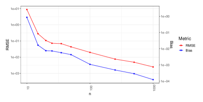
Figure 3: Empirical Bias and RMSE of the first singular value of an $n\times n$ matrix comprising a rank three matrix and an error matrix (Both the horizontal and vertical axes are in logarithmic scale)

3 Experimental Results

3.1 Experimental Setup

As explained in Section 1, we focus on comparing the proposed rSVDdpd method primarily with the existing robust PCA algorithms for background modelling. As most of the recent advancements in the robust PCA based approaches concern themselves with reducing the computational complexity of the optimization algorithm rather than significantly improving the performance of the background modelling estimates, we restrict our attention to the major robust PCA approaches and the corresponding seminal algorithms. These include the exact Principal Component Pursuit (PCP) via Augmented Lagrangian Method (ALM) (21), inexact ALM via alternating direction (31), Outlier Pursuit (OP) (33), Sparse Regularized PCP (SRPCP) (35) and Variational Bayesian method (VB) (34). In addition, we also consider one statistical algorithm Go Decomposition (GoDec) (54) and an incremental algorithm, namely the Grassmannian Robust Adaptive Subspace Tracking Algorithm (GRASTA) (55; 37). While the first set of algorithms work with a batch of multiple frames at a time to extract the foreground content, the last algorithm GRASTA is online in nature, it processes one frame of the video at a time and uses the information from the previous frames to extract foreground of the current video frame. R implementation of rSVDdpd and exact PCP method for robust PCA are available in the rSVDdpd (56) and the RPCA (57) packages, respectively. The MATLAB implementations of the rest of the algorithms are available in Background Subtraction Website which have been converted to R implementation to compare these methods on a level ground. All the experiments have been done in an Azure virtual machine with 4 vCPUs and 32 GB of RAM.

To compare these methods and measure performances, we consider the Background Models Challenge benchmark dataset (58). This benchmark dataset has also been used in earlier studies to provide a detailed comparison of several background modelling algorithms (20). The dataset contains $20$ synthetic videos with ground truth foreground masks. The synthetic videos are generated by SIVIC software and closely resemble different kinds of natural tampering present in real-life video surveillance data such as noises, artifacts, shadows, change of illumination, presence of fog and rain, etc. The whole set of videos comprises to two kinds of backgrounds, one of a straight street highway (Street), while the other contains the simulated video footage of a traffic junction (Rotary). Among these $10$ pairs of videos, we use the first of each pair to train the parameters of these algorithms and use the second of each pair to test the performance of the respective trained models. Due to the computational limitations of the existing algorithms, we train each of the algorithms using batches of $120$ frames from the videos at a time and find the optimal parameter with the best $F1$-measure. The $F1$-measure is the harmonic mean of the precision and recall, which is generally accepted as a robust measure of the performance of any classification algorithm. Using the ground truth mask provided in the dataset, we calculate the precision as the ratio of the correctly predicted foreground pixels and the predicted foreground pixels, while the recall is calculated as the ratio of the correctly predicted foreground pixels and the number of pixels assigned to the foreground content in the ground truth video.

3.2 Discussions of Results for the Benchmark Dataset

Table 1: Time taken (in seconds) for processing a single frame for different background modelling algorithms
(Algorithms are in descending order of speed)

Method	Average Time	Std. dev.
	(in seconds/frame)	(in seconds/frame)
GRASTA (37)	0.37	0.01
rSVDdpd (ours)	2.86	0.84
VB (34)	7.06	1.39
GoDec (54)	12.06	0.29
OP (33)	23.42	0.22
ALM (31)	34.85	7.40
SRPCP (35)	54.25	9.12
RPCA (21)	136.41	27.26

Table 2: Benchmark Results for different variants of the Street Video (Video number Vi1j denotes $i$-th variant of the Street Video and $j=1$ or $2$ denote the training and the testing video respectively); In each column, bold symbols indicate the best performing algorithm with respect to the $F_{1}$ measure.

Method	Measures	V111	V112	V211	V212	V311	V312	V411	V412	V511	V512
RPCA (21)	Precision	0.766	0.741	0.788	0.764	0.751	0.761	0.983	0.784	0.617	0.487
	Recall	0.768	0.767	0.747	0.744	0.7	0.698	0.655	0.675	0.568	0.49
	F1	0.767	0.754	0.767	0.754	0.725	0.728	0.787	0.726	0.592	0.489
ALM (31)	Precision	0.766	0.741	0.811	0.765	0.752	0.762	0.984	0.785	0.626	0.486
	Recall	0.768	0.767	0.729	0.745	0.7	0.698	0.655	0.675	0.568	0.49
	F1	0.767	0.754	0.768	0.755	0.725	0.729	0.787	0.726	0.595	0.488
SRPCP (35)	Precision	0.766	0.741	0.811	0.765	0.752	0.762	0.984	0.785	0.626	0.486
	Recall	0.768	0.767	0.729	0.745	0.7	0.698	0.657	0.675	0.568	0.49
	F1	0.767	0.754	0.768	0.755	0.725	0.729	0.788	0.726	0.595	0.488
VB (34)	Precision	0.774	0.749	0.809	0.764	0.75	0.761	0.985	0.781	0.323	0.38
	Recall	0.767	0.766	0.729	0.745	0.701	0.698	0.654	0.649	0.48	0.435
	F1	0.77	0.757	0.767	0.754	0.725	0.728	0.786	0.709	0.386	0.405
OP (33)	Precision	0.783	0.776	0.825	0.794	0.757	0.837	0.985	0.797	0.686	0.619
	Recall	0.769	0.748	0.727	0.723	0.699	0.532	0.653	0.643	0.601	0.5
	F1	0.776	0.762	0.773	0.757	0.727	0.65	0.785	0.712	0.641	0.553
GoDec (54)	Precision	0.844	0.8	0.786	0.762	0.749	0.771	0.981	0.51	0.205	0.414
	Recall	0.686	0.676	0.748	0.745	0.701	0.595	0.654	0.443	0.364	0.214
	F1	0.757	0.733	0.767	0.754	0.724	0.672	0.785	0.474	0.263	0.282
GRASTA (37)	Precision	0.646	0.766	0.613	0.758	0.764	0.89	0.987	0.165	0.338	0.374
	Recall	0.764	0.644	0.727	0.712	0.613	0.282	0.652	0.189	0.395	0.367
	F1	0.700	0.699	0.665	0.734	0.68	0.428	0.785	0.176	0.364	0.371
rSVDdpd ((ours)	Precision	0.783	0.776	0.78	0.769	0.753	0.842	0.987	0.8	0.785	0.626
	Recall	0.772	0.768	0.769	0.746	0.699	0.683	0.653	0.735	0.601	0.497
	F1	0.777	0.772	0.774	0.757	0.725	0.754	0.787	0.766	0.681	0.553

Table 3: Benchmark Results for different variants of the Rotary Video (Video number Vi2j denotes $i$-th variant of the Rotary Video and $j=1$ or $2$ denote the training and the testing video respectively); In each column, bold symbols indicate the best performing algorithm with respect to the $F_{1}$ measure.

Method	Measures	V121	V122	V221	V222	V321	V322	V421	V422	V521	V522
RPCA (21)	Precision	0.771	0.771	0.792	0.795	0.781	0.781	0.893	0.698	0.425	0.496
	Recall	0.771	0.769	0.733	0.738	0.656	0.659	0.612	0.547	0.592	0.599
	F1	0.771	0.77	0.761	0.766	0.713	0.714	0.726	0.614	0.495	0.542
ALM (31)	Precision	0.772	0.771	0.792	0.796	0.781	0.781	0.898	0.698	0.422	0.491
	Recall	0.771	0.769	0.733	0.738	0.656	0.659	0.611	0.546	0.592	0.599
	F1	0.772	0.77	0.761	0.766	0.713	0.714	0.727	0.613	0.493	0.54
SRPCP (35)	Precision	0.772	0.771	0.792	0.796	0.781	0.781	0.898	0.698	0.422	0.491
	Recall	0.771	0.769	0.733	0.738	0.656	0.659	0.611	0.546	0.592	0.599
	F1	0.772	0.77	0.761	0.766	0.713	0.715	0.727	0.613	0.493	0.54
VB (34)	Precision	0.772	0.772	0.793	0.797	0.776	0.773	0.904	0.683	0.447	0.483
	Recall	0.771	0.769	0.733	0.738	0.658	0.661	0.611	0.518	0.526	0.527
	F1	0.772	0.77	0.762	0.766	0.712	0.713	0.729	0.589	0.483	0.504
OP (33)	Precision	0.806	0.79	0.792	0.802	0.751	0.797	0.883	0.655	0.551	0.544
	Recall	0.728	0.733	0.713	0.7	0.657	0.468	0.611	0.517	0.467	0.488
	F1	0.765	0.76	0.75	0.749	0.701	0.59	0.722	0.577	0.506	0.514
GoDec (54)	Precision	0.815	0.795	0.758	0.762	0.737	0.796	0.987	0.57	0.502	0.512
	Recall	0.624	0.688	0.734	0.739	0.661	0.539	0.57	0.587	0.476	0.5
	F1	0.707	0.738	0.746	0.75	0.697	0.642	0.723	0.578	0.488	0.506
GRASTA (37)	Precision	0.82	0.56	0.604	0.797	0.758	0.762	0.892	0.45	0.334	0.346
	Recall	0.684	0.692	0.69	0.7	0.628	0.301	0.61	0.283	0.603	0.611
	F1	0.746	0.619	0.644	0.748	0.687	0.432	0.724	0.347	0.43	0.442
rSVDdpd (ours)	Precision	0.772	0.784	0.798	0.805	0.735	0.685	0.901	0.697	0.742	0.634
	Recall	0.792	0.769	0.729	0.733	0.686	0.718	0.65	0.58	0.56	0.586
	F1	0.781	0.776	0.762	0.767	0.710	0.702	0.755	0.633	0.638	0.609

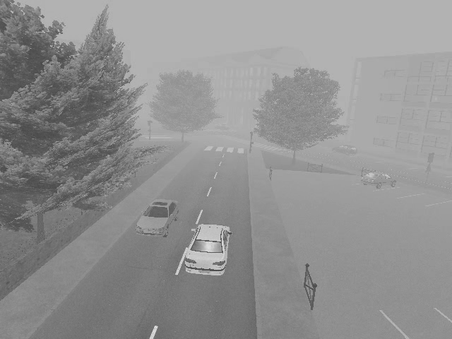
(a)

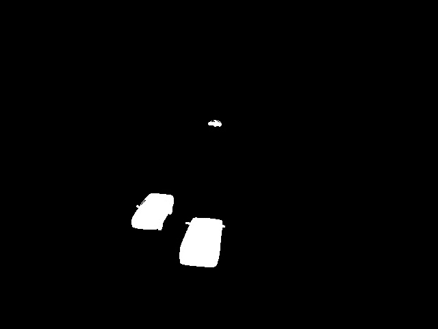
(b)

(c)

(d)

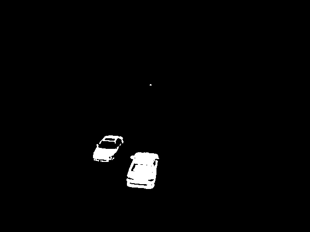
(e)

(f)

(g)

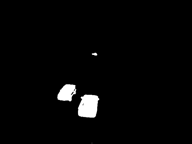
(h)

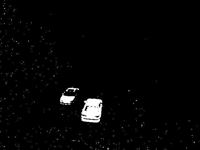
(i)

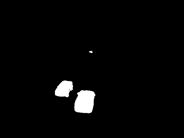
(j)

Figure 4: One frame of the street video (a), ground truth (b) and estimated foreground mask from exact RPCA (c), inexact ALM (d), SRPCP (e), Variational Bayes (f), Outlier Pursuit (g), GoDec (h), GRASTA (i) and rSVDdpd (j) algorithms. Enlarged better quality images are available online at https://subroy13.github.io/rsvddpd-home/.

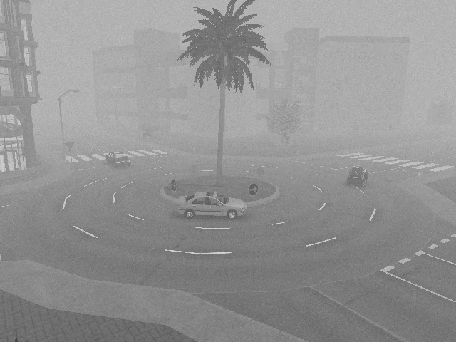
(a)

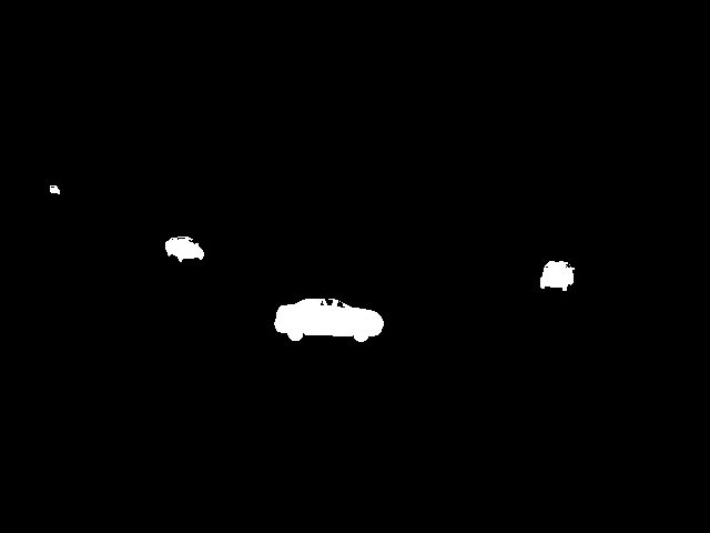
(b)

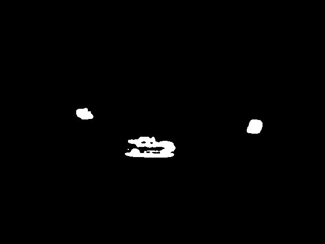
(c)

(d)

(e)

(f)

(g)

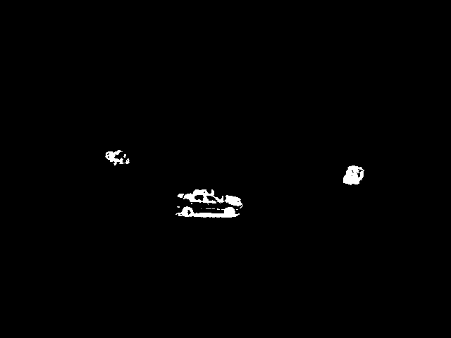
(h)

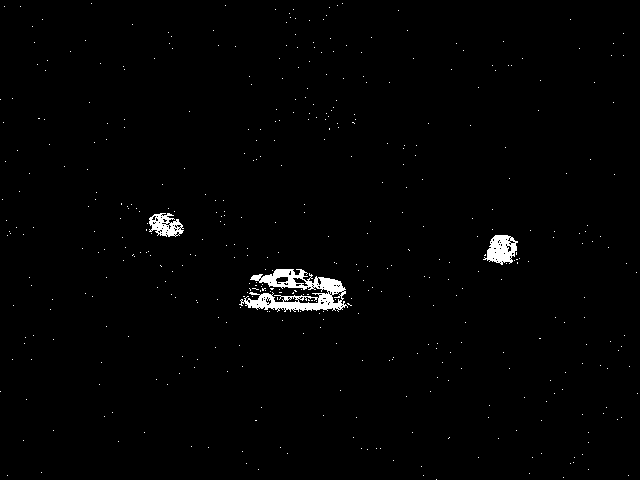
(i)

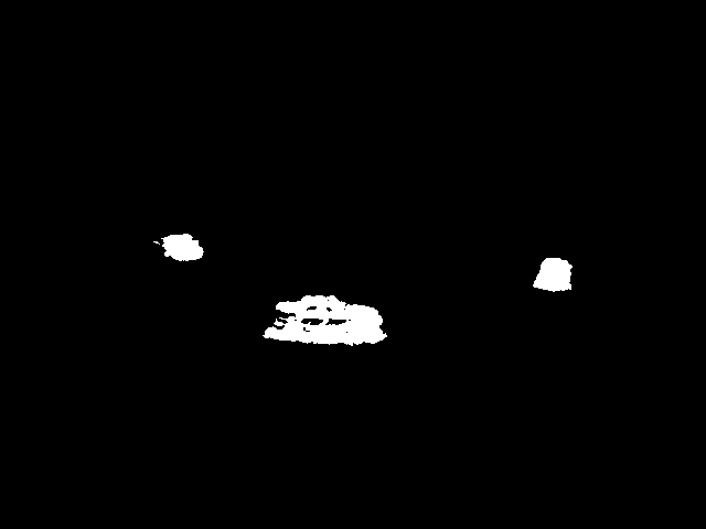
(j)

Figure 5: One frame of the rotary video (a), ground truth (b) and estimated foreground mask from exact RPCA (c), inexact ALM (d), SRPCP (e), Variational Bayes (f), Outlier Pursuit (g), GoDec (h), GRASTA (i) and rSVDdpd (j) algorithms. Enlarged better quality images are available online at https://subroy13.github.io/rsvddpd-home/.

In Table 1, we summarize the average and the standard deviation of the time taken per frame (in seconds) by each of the algorithms to converge and separate the background and foreground content. Only GRASTA and rSVDdpd algorithms complete the foreground extraction task in a reasonable amount of time to be useful in real-time video surveillance and object tracking. In contrast, the exact robust PCA method takes an enormous amount of time to converge, more than $2$ minutes per frame, thus destroying its practical utility. The variants of robust PCA, i.e., inexact ALM and SRPCP methods reduce the computational time significantly, but they are still not on par with the speed of rSVDdpd or GRASTA algorithms. This computational performance gain of rSVDdpd can be further boosted through the highly parallelizable structure of the iteration rules (2.11), where each component $a_{i}$ (or $b_{j}$) of the singular vectors can be updated simultaneously. This empirically demonstrates how rSVDdpd solves the problem of scalability of the video surveillance background modelling methods and achieves high parallelizability.

In Table 2 and Table 3, we summarize the performances of the different algorithms for foreground detection on the benchmark datasets. Clearly, the proposed rSVDdpd algorithm outperforms all the existing algorithms under consideration for almost all the benchmark videos. For some of the videos where rSVDdpd does not achieve the best $F1$-measure, the difference in $F1$-measure compared to the best output is too small to visually distinguish the extracted foregrounds. It turns out that the inexact ALM method and the SRPCP method have similar performances as the exact robust PCA algorithm, while the OP and VB methods perform better than these only in some specific scenarios, in particular when the background shows some continuous natural movement of the trees. Both GoDec and GRASTA algorithms do not work well under these situations. In comparison, the rSVDdpd algorithm is able to tackle all these scenarios by allowing the background matrix $\boldsymbol{L}$ to be of rank more than one.

As seen from the above discussions, the rSVDdpd algorithm achieves superior or near-optimal compared to the existing robust PCA and background modelling methods by spending only a fraction of computational time. GRASTA, the only algorithm that is faster than the proposed rSVDdpd (indeed, faster than all other algorithms compared), achieves this speed at the cost of a very poor performance under different kinds of noises present in the real-life video data. A fast algorithm with little performance guarantee can only be of limited use. For instance, GRASTA performs worse than all the algorithms compared for video 412 and 422 of Table 2 and 3 respectively. These two videos have small amount of noises added throughout the video and fog and haze appear in between for some consecutive frames as the outlying observations. While the improvement (rSVDdpd over GRASTA) is not necessarily absolute in all the other cases, many other videos (such as 312, 511, 512 in Table 2 and 322, 521, 522 in Table 3) show that the improvement is substantial in most cases. And in each of these cases the rSVDdpd is either the top performer, or is in the neighborhood of the best. The degree may vary by small amounts in the other videos, but the general pattern holds true. The rSVDdpd holds its own even when practically all the other algorithms show a largely degraded performance, e.g., as in the case of video 512. Also, rSVDdpd is the second best in our examined set in terms of speed (see Table 1), clearly beats the GRASTA algorithm in terms of performance accuracy, is competitive or better than all the other algorithms in terms of performance accuracy, and is 3 to 50 times faster than all the other algorithms compared except GRASTA. Thus, the proposed rSVDdpd keeps an optimal balance between speed and accuracy without losing much in both of these aspects.

Due to space constraint, we demonstrate the estimated foreground masks as obtained from only two frames of the two videos, using different existing algorithms and the proposed rSVDdpd algorithm in Figures 4 and 5. As shown in these figures, both the exact robust PCA method and the rSVDdpd method lead to visually indistinguishable results; however rSVDdpd achieves the same at the cost of a significantly reduced computational time compared to the exact robust PCA algorithm. The inexact ALM, SRPCP and VB methods, which converge faster than the exact robust PCA method, sometimes find it difficult to extract the foreground object in the presence of clouds and fog. The proposed rSVDdpd algorithm can efficiently work in all these situations by considering a rank-one approximation of the background matrix $\boldsymbol{L}$. Due to the use of the robust MDPDE, any moving foreground objects are also captured through the rSVDdpd algorithm even when the cloud or the fog blends the foreground’s grayscale intensity with the background’s grayscale intensity. The other alternative competing methods for video surveillance, namely GRASTA and GoDec estimate a noisy background in general. Although these noises remain imperceptible at first, they result in a more noisy foreground, and such noisy pixels sometimes become visible in the thresholded foreground mask. As demonstrated earlier in Figure 1, the rSVDdpd algorithm outputs a noise free background even if the original video frame is noisy, thus eliminating such undesirable behaviours. The results obtained from all the videos under these benchmark datasets are presented, for brevity, on the accompanying rSVDdpd webpage https://subroy13.github.io/rsvddpd-home/ (See Section 3.4 for details).

3.3 Application to a Large Scale Camera Tampering Video Surveillance Dataset

As mentioned in Section 1, video surveillance under the presence of camera tampering is a very challenging and useful problem. With the problem of camera tampering detection (i.e., classification of tampered frames) in mind, (2) have compiled a comprehensive large-scale dataset called UHCTD (University of Houston Camera Tampering Detection Dataset), which we choose here for the purpose of illustration of performances of these background modelling algorithms under real-life video surveillance data. The dataset contains surveillance videos of over 288 hours ranging across 6 days from two cameras. Three types of camera tampering methods have been synthesized in the dataset; (a) covered, (b) defocused, and, (c) moved (see more details in (2)). These tamperings are done uniformly over the data to capture changing illumination between day and night.

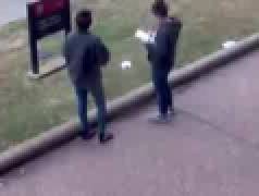
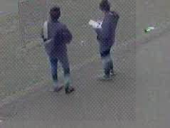
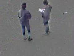
(a)

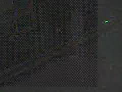
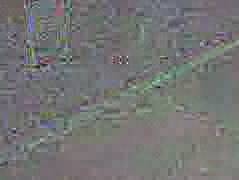
(b)

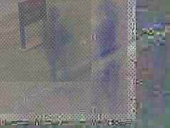
(c)

Figure 6: True video frames and the estimated foreground by usual SVD, rSVDdpd, ALM and GoDec algorithms (Left to Right) for frame 5, 50, 75 in UHCTD Day 1 Camera B dataset. Enlarged better quality images are available online at https://subroy13.github.io/rsvddpd-home/

Figure 6 depicts the true frames along with the estimated foregrounds obtained from the usual SVD, robust rSVDdpd, robust PCA via ALM and GoDec algorithms. The estimated backgrounds obtained from other robust PCA methods are visually similar to the output of the ALM algorithm and hence are omitted here. In this surveillance scene from Camera B (2), a noisy image is synthesized to obstruct the view of the camera. The background estimated from the usual SVD shows a clear indication of the noise even in the frames where camera tampering is not induced, and such an effect is amplified further by the presence of shadow-like artifacts in the estimated background content. Such an effect is also prevalent across the existing techniques. In comparison, the background estimated via the proposed rSVDdpd algorithm removes such artifacts and is less affected by the tampering. This robustness property can also be seen in the estimated foreground content, when the true frame is only the non-tampered background, the proposed rSVDdpd outputs foreground content as a very dark black image without any distinguishing feature as desired.

3.4 Further Illustrations

Further illustrations of the performance of the proposed rSVDdpd over the existing comparative algorithms are available in the accompanying rSVDdpd Website https://subroy13.github.io/rsvddpd-home/. The website contains an extended abstract, the necessary R codes, and the detailed description and the images and videos of the estimated foreground of the benchmark datasets and the tampered videos from UHCTD dataset. The proposed method is incorporated in the R-package rSVDdpd and made publicly available via CRAN repository (https://cran.r-project.org/web/packages/rsvddpd/index.html).

4 Conclusion

In this paper, we had set out to solve the extremely important problem of modelling video surveillance background content robustly, and we trust we have achieved that with the help of a novel algorithm which performs the singular value decomposition robustly. This, we believe, has been adequately demonstrated in our examples. Several existing methods such as GRASTA, MOG and GoDec algorithms which are extensively used for this task, have been shown to have degraded performance in presence of both natural noise and camera tampering (7; 22). The more recent approaches based on robust PCA perform better than these algorithms, although at the cost of high computational complexity (20). In comparison, our novel robust singular value decomposition technique based on density power divergence can provide a faster alternative to the robust PCA based methods for the statistical background modelling problems (without compromising robustness). Through a comparative study based on the benchmark dataset, we have demonstrated that the proposed rSVDdpd algorithm is extremely fast and parallelizable, and achieves a performance that is as good as these existing state of the art algorithms. Moreover, in the presence of natural or artificial camera tampering, which is ubiquitous in real-life video surveillance data, the proposed rSVDdpd algorithm yields more reliable background estimates of the non-tampered frames than existing algorithms.

The proposed rSVDdpd algorithm is used on a batch of video frames. However, an online version of rSVDdpd algorithm could be extremely useful to be used in a real-time video surveillance application, where the low rank component can automatically update as soon as new video frames come in. Another direction of future research could be to develop a data-driven method to estimate the rank of the background matrix $\boldsymbol{L}$, which will control the amount of slowly moving objects in the background content. Also, as SVD is abundantly used for analyzing high dimensional data, it would be useful to know the range of applications where the proposed rSVDdpd can replace the standard SVD to counter data contamination. We hope to take up these problems in the future.

References

- Garcia-Garcia et al. [2020] Belmar Garcia-Garcia, Thierry Bouwmans, and Alberto Jorge Rosales Silva. Background Subtraction in Real Applications: Challenges, Current Models and Future Directions. Computer Science Review, 35:100204, 2020. ISSN 1574-0137. doi: https://doi.org/10.1016/j.cosrev.2019.100204. URL https://www.sciencedirect.com/science/article/pii/S1574013718303101.
- Mantini and Shah [2019a] Pranav Mantini and Shishir K. Shah. UHCTD: A Comprehensive Dataset for Camera Tampering Detection. In 2019 16th IEEE International Conference on Advanced Video and Signal Based Surveillance (AVSS), pages 1–8, 2019a. doi: 10.1109/AVSS.2019.8909856.
- Mantini and Shah [2019b] Pranav Mantini and Shishir K Shah. Camera Tampering Detection using Generative Reference Model and Deep Learned Features. In VISIGRAPP (5: VISAPP), pages 85–95, 2019b.
- Sitara and Mehtre [2019] K. Sitara and B. M. Mehtre. Automated camera sabotage detection for enhancing video surveillance systems. Multimedia Tools and Applications, 78(5):5819–5841, Mar 2019. ISSN 1573-7721. doi: 10.1007/s11042-018-6165-4. URL https://doi.org/10.1007/s11042-018-6165-4.
- Lee and Hedley [2002] B Lee and M Hedley. Background estimation for video surveillance. In Proc. of the Image & Vision Computing New Zealand, IVCNZ, pages 315–320, Auckland, NZ, 2002. URL http://hdl.handle.net/102.100.100/199802?index=1.
- McIvor [2000] Alan M McIvor. Background Subtraction Techniques. Proc. of Image and Vision Computing, 4:3099–3104, 2000.
- Bouwmans et al. [2010] Thierry Bouwmans, Fida El Baf, and Bertrand Vachon. Statistical background modeling for foreground detection: A survey, pages 181–199. World Scientific, 2010. doi: 10.1142/9789814273398_0008. URL https://www.worldscientific.com/doi/abs/10.1142/9789814273398_0008.
- Lee [2005] Dar-Shyang Lee. Effective Gaussian mixture learning for video background subtraction. IEEE Transactions on Pattern Analysis and Machine Intelligence, 27(5):827–832, 2005. doi: 10.1109/TPAMI.2005.102.
- Subudhi et al. [2022] Badri Narayan Subudhi, Manoj Kumar Panda, T. Veerakumar, Vinit Jakhetiya, and S. Esakkirajan. Kernel-Induced Possibilistic Fuzzy Associate Background Subtraction for Video Scene. IEEE Transactions on Computational Social Systems, pages 1–12, 2022. doi: 10.1109/TCSS.2021.3137306.
- Zhao et al. [2012] Zhenjie Zhao, Thierry Bouwmans, Xuebo Zhang, and Yongchun Fang. A Fuzzy Background Modeling Approach for Motion Detection in Dynamic Backgrounds. In International Conference on Multimedia and Signal Processing, pages 177–185. Springer, 2012.
- Munteanu et al. [2015] Oana Munteanu, Thierry Bouwmans, El-hadi ZAHZAH, and Radu Vasiu. The detection of moving objects in video by background subtraction using Dempster-Shafer theory. Scientific Bulletin of the Politehnica University of Timisoara, Transactions on Electronics and Communications, ISSN 1583-3380, 60(74):45–52, 03 2015.
- Zhang et al. [2016] Hongyi Zhang, Sashank J Reddi, and Suvrit Sra. Riemannian SVRG: Fast stochastic optimization on Riemannian manifolds. Advances in Neural Information Processing Systems, 29:4592–4600, 2016.
- Vaswani et al. [2018] Namrata Vaswani, Thierry Bouwmans, Sajid Javed, and Praneeth Narayanamurthy. Robust Subspace Learning: Robust PCA, Robust Subspace Tracking, and Robust Subspace Recovery. IEEE Signal Processing Magazine, 35(4):32–55, July 2018. doi: 10.1109/MSP.2018.2826566. URL https://hal.archives-ouvertes.fr/hal-01790782.
- Maddalena and Petrosino [2012] Lucia Maddalena and Alfredo Petrosino. The SOBS algorithm: What are the limits? In 2012 IEEE Computer Society Conference on Computer Vision and Pattern Recognition Workshops, pages 21–26, 2012. doi: 10.1109/CVPRW.2012.6238922.
- Giraldo et al. [2021] Jhony H. Giraldo, Sajid Javed, Naoufel Werghi, and Thierry Bouwmans. Graph CNN for Moving Object Detection in Complex Environments from Unseen Videos. In 2021 IEEE/CVF International Conference on Computer Vision Workshops (ICCVW), pages 225–233, 2021. doi: 10.1109/ICCVW54120.2021.00030.
- Mandal and Vipparthi [2022] Murari Mandal and Santosh Kumar Vipparthi. An Empirical Review of Deep Learning Frameworks for Change Detection: Model Design, Experimental Frameworks, Challenges and Research Needs. Trans. Intell. Transport. Sys., 23(7):6101–6122, jul 2022. ISSN 1524-9050. doi: 10.1109/TITS.2021.3077883. URL https://doi.org/10.1109/TITS.2021.3077883.
- Messelodi et al. [2005] Stefano Messelodi, Carla Maria Modena, N. Segata, and Michele Zanin. A Kalman Filter Based Background Updating Algorithm Robust to Sharp Illumination Changes. In ICIAP, 2005.
- Stagliano et al. [2015] Alessandra Stagliano, Nicoletta Noceti, Alessandro Verri, and Francesca Odone. Online Space-Variant Background Modeling With Sparse Coding. IEEE Transactions on Image Processing, 24(8):2415–2428, 2015. doi: 10.1109/TIP.2015.2421435.
- Giraldo et al. [2022] Jhony H. Giraldo, Sajid Javed, and Thierry Bouwmans. Graph Moving Object Segmentation. IEEE Transactions on Pattern Analysis and Machine Intelligence, 44(5):2485–2503, 2022. doi: 10.1109/TPAMI.2020.3042093.
- Bouwmans and Zahzah [2014] Thierry Bouwmans and El Hadi Zahzah. Robust PCA via Principal Component Pursuit: A Review for a Comparative Evaluation in Video Surveillance. Computer Vision and Image Understanding, 122:22–34, 2014. ISSN 1077-3142. doi: https://doi.org/10.1016/j.cviu.2013.11.009. URL https://www.sciencedirect.com/science/article/pii/S1077314213002294.
- Candès et al. [2011] Emmanuel J. Candès, Xiaodong Li, Yi Ma, and John Wright. Robust Principal Component Analysis? J. ACM, 58(3), 6 2011. ISSN 0004-5411. doi: 10.1145/1970392.1970395. URL https://doi.org/10.1145/1970392.1970395.
- Bouwmans [2014] Thierry Bouwmans. Traditional and Recent Approaches in Background Modeling for Foreground Detection: An overview. Computer Science Review, 11-12:31–66, 2014. ISSN 1574-0137. doi: https://doi.org/10.1016/j.cosrev.2014.04.001. URL https://www.sciencedirect.com/science/article/pii/S1574013714000033.
- Caseiro et al. [2010a] Rui Caseiro, Joao F. Henriques, and Jorge Batista. Foreground Segmentation via Background Modeling on Riemannian Manifolds. In 2010 20th International Conference on Pattern Recognition, pages 3570–3574. IEEE, 2010a. doi: 10.1109/ICPR.2010.871.
- Caseiro et al. [2010b] Rui Caseiro, Jorge Batista, and Pedro Martins. Background Modelling on Tensor Field for Foreground Segmentation. In Proceedings of the British Machine Vision Conference, pages 96.1–96.12. BMVA Press, 2010b. ISBN 1-901725-40-5. doi:10.5244/C.24.96.
- Ha et al. [2020] Synh Viet-Uyen Ha, Nhat Minh Chung, Hung Ngoc Phan, and Cuong Tien Nguyen. TensorMoG: A Tensor-Driven Gaussian Mixture Model with Dynamic Scene Adaptation for Background Modelling. Sensors, 20(23), 2020. ISSN 1424-8220. doi: 10.3390/s20236973. URL https://www.mdpi.com/1424-8220/20/23/6973.
- Kumar et al. [2011] Nishith Kumar, Mohammed Nasser, and Subaran Chandra Sarker. A new singular value decomposition based robust graphical clustering technique and its application in climatic data. Journal of Geography and Geology, 3(1):227, 2011.
- Hawkins et al. [2001] Douglas M. Hawkins, Li Liu, and S. Stanley Young. Robust Singular Value Decomposition. Technical Report 122, National Institute of Statistical Sciences (NISS), 12 2001.
- Liu et al. [2003] Li Liu, Douglas M Hawkins, Sujoy Ghosh, and S Stanley Young. Robust Singular Value Decomposition Analysis of Microarray Data. Proceedings of the National Academy of Sciences, 100(23):13167–13172, 2003.
- Babanezhad et al. [2019] Reza Babanezhad, Issam H. Laradji, Alireza Shafaei, and Mark Schmidt. MASAGA: A Linearly-Convergent Stochastic First-Order Method for Optimization on Manifolds. In Michele Berlingerio, Francesco Bonchi, Thomas Gärtner, Neil Hurley, and Georgiana Ifrim, editors, Machine Learning and Knowledge Discovery in Databases, pages 344–359, Cham, 2019. Springer International Publishing. ISBN 978-3-030-10928-8.
- Xue et al. [2019] Niannan Xue, Jiankang Deng, Shiyang Cheng, Yannis Panagakis, and Stefanos Zafeiriou. Side Information for Face Completion: A Robust PCA Approach. IEEE Transactions on Pattern Analysis and Machine Intelligence, 41(10):2349–2364, 2019. doi: 10.1109/TPAMI.2019.2902556.
- Shen et al. [2014] Y. Shen, Z. Wen, and Y. Zhang. Augmented Lagrangian Alternating Direction Method for Matrix Separation based on Low-rank Factorization. Optimization Methods and Software, 29(2):239–263, 2014. doi: 10.1080/10556788.2012.700713. URL https://doi.org/10.1080/10556788.2012.700713.
- Yi et al. [2016] Xinyang Yi, Dohyung Park, Yudong Chen, and Constantine Caramanis. Fast Algorithms for Robust PCA via Gradient Descent. In Proceedings of the 30th International Conference on Neural Information Processing Systems, NIPS’16, pages 4159–4167, Red Hook, NY, USA, 2016. Curran Associates Inc. ISBN 9781510838819.
- Xu et al. [2012] Huan Xu, Constantine Caramanis, and Sujay Sanghavi. Robust PCA via Outlier Pursuit. IEEE Transactions on Information Theory, 58(5):3047–3064, 2012. doi: 10.1109/TIT.2011.2173156.
- Babacan et al. [2012] S. Derin Babacan, Martin Luessi, Rafael Molina, and Aggelos K. Katsaggelos. Sparse Bayesian Methods for Low-Rank Matrix Estimation. IEEE Transactions on Signal Processing, 60(8):3964–3977, 2012. doi: 10.1109/TSP.2012.2197748.
- Liu et al. [2017] Jing Liu, Pamela C Cosman, and Bhaskar D Rao. Sparsity Regularized Principal Component Pursuit. In 2017 IEEE International Conference on Acoustics, Speech and Signal Processing (ICASSP), pages 4431–4435. IEEE, 2017.
- Narayanamurthy and Vaswani [2018] Praneeth Narayanamurthy and Namrata Vaswani. A Fast and Memory-Efficient Algorithm for Robust PCA (MEROP). In 2018 IEEE International Conference on Acoustics, Speech and Signal Processing (ICASSP), pages 4684–4688, 2018. doi: 10.1109/ICASSP.2018.8461540.
- He et al. [2012] Jun He, Laura Balzano, and Arthur Szlam. Incremental gradient on the Grassmannian for online foreground and background separation in subsampled video. In 2012 IEEE Conference on Computer Vision and Pattern Recognition, pages 1568–1575. IEEE, 2012. doi: 10.1109/CVPR.2012.6247848.
- Rodriguez and Wohlberg [2016] Paul Rodriguez and Brendt Wohlberg. Incremental Principal Component Pursuit for Video Background Modeling. Journal of Mathematical Imaging and Vision, 55(1):1–18, May 2016. ISSN 0924-9907. doi: 10.1007/s10851-015-0610-z. URL https://doi.org/10.1007/s10851-015-0610-z.
- Javed et al. [2019] Sajid Javed, Arif Mahmood, Somaya Al-Maadeed, Thierry Bouwmans, and Soon Ki Jung. Moving Object Detection in Complex Scene Using Spatiotemporal Structured-Sparse RPCA. IEEE Transactions on Image Processing, 28(2):1007–1022, 2019. doi: 10.1109/TIP.2018.2874289.
- Zhu et al. [2020] Lin Zhu, Xiurong Jiang, Jianing Li, Yuanhong Hao, and Yonghong Tian. Motion-Aware Structured Matrix Factorization for Foreground Detection in Complex Scenes. ACM Trans. Multimedia Comput. Commun. Appl., 16(4), dec 2020. ISSN 1551-6857. doi: 10.1145/3407188. URL https://doi.org/10.1145/3407188.
- Cai et al. [2019] HanQin Cai, Jian-Feng Cai, and Ke Wei. Accelerated Alternating Projections for Robust Principal Component Analysis. The Journal of Machine Learning Research, 20(1):685–717, 2019.
- Xiu et al. [2020] Xianchao Xiu, Ying Yang, Lingchen Kong, and Wanquan Liu. Laplacian regularized robust principal component analysis for process monitoring. Journal of Process Control, 92:212–219, 2020. ISSN 0959-1524. doi: https://doi.org/10.1016/j.jprocont.2020.06.011. URL https://www.sciencedirect.com/science/article/pii/S095915242030247X.
- Jain and Kar [2017] Prateek Jain and Purushottam Kar. Non-convex Optimization for Machine Learning. Foundations and Trends® in Machine Learning, 10(3-4):142–336, 2017. doi: 10.1561/2200000058. URL https://doi.org/10.1561%2F2200000058.
- Duan et al. [2022] Ran Duan, Hongxun Wu, and Renfei Zhou. Faster Matrix Multiplication via Asymmetric Hashing, 2022. URL https://arxiv.org/abs/2210.10173.
- Basu et al. [1998] Ayanendranath Basu, Ian R. Harris, Nils L. Hjort, and M. C. Jones. Robust and Efficient Estimation by Minimising a Density Power Divergence. Biometrika, 85(3):549–559, 1998. ISSN 00063444. URL http://www.jstor.org/stable/2337385.
- Ghosh and Basu [2013] Abhik Ghosh and Ayanendranath Basu. Robust estimation for independent non-homogeneous observations using density power divergence with applications to linear regression. Electronic Journal of Statistics, 7(none):2420 – 2456, 2013. doi: 10.1214/13-EJS847. URL https://doi.org/10.1214/13-EJS847.
- Xiong and Zhu [2021] Lanyu Xiong and Fukang Zhu. Minimum Density Power Divergence Estimator for Negative Binomial Integer-Valued GARCH Models. Communications in Mathematics and Statistics, pages 1–29, April 2021. doi: 10.1007/s40304-020-00221-8. URL https://doi.org/10.1007%2Fs40304-020-00221-8.
- Mahadevan and Vasconcelos [2010] Vijay Mahadevan and Nuno Vasconcelos. Spatiotemporal Saliency in Dynamic Scenes. IEEE Transactions on Pattern Analysis and Machine Intelligence, 32(1):171–177, 2010. ISSN 0162-8828. doi: http://doi.ieeecomputersociety.org/10.1109/TPAMI.2009.112. URL http://www.svcl.ucsd.edu/projects/background_subtraction/ucsdbgsub_dataset.htm.
- Rey [2007] William Rey. Total Singular Value Decomposition. Robust SVD, Regression and Location-Scale, 2007.
- Owen and Perry [2009] Art B. Owen and Patrick O. Perry. Bi-Cross-Validation of the SVD and the Nonnegative Matrix Factorization. The Annals of Applied Statistics, 3(2):564–594, 2009. ISSN 19326157, 19417330. URL http://www.jstor.org/stable/30244256.
- Giraud et al. [2005] L. Giraud, J. Langou, and M. Rozloznik. The loss of orthogonality in the Gram-Schmidt orthogonalization process. Computers & Mathematics with Applications, 50(7):1069–1075, 2005. ISSN 0898-1221. doi: https://doi.org/10.1016/j.camwa.2005.08.009. URL https://www.sciencedirect.com/science/article/pii/S0898122105003366. Numerical Methods and Computational Mechanics.
- Huang et al. [2009] Jianhua Z. Huang, Haipeng Shen, and Andreas Buja. The Analysis of Two-Way Functional Data Using Two-Way Regularized Singular Value Decompositions. Journal of the American Statistical Association, 104(488):1609–1620, 2009. doi: 10.1198/jasa.2009.tm08024. URL https://doi.org/10.1198/jasa.2009.tm08024.
- Roy et al. [2023] Subhrajyoty Roy, Ayanendranath Basu, and Abhik Ghosh. Analysis of the rsvddpd algorithm: A robust singular value decomposition method using density power divergence. arXiv preprint arXiv:2307.10591, 2023.
- Zhou and Tao [2011] Tianyi Zhou and Dacheng Tao. GoDec: Randomized Low-Rank & Sparse Matrix Decomposition in Noisy Case. In Proceedings of the 28th International Conference on International Conference on Machine Learning, ICML’11, page 33–40, Madison, WI, USA, 2011. Omnipress. ISBN 9781450306195.
- He et al. [2011] Jun He, Laura Balzano, and John Lui. Online Robust Subspace Tracking from Partial Information. arXiv preprint arXiv:1109.3827, 2011.
- Roy [2021] Subhrajyoty Roy. rsvddpd: Robust Singular Value Decomposition using Density Power Divergence, 2021. URL https://CRAN.R-project.org/package=rsvddpd. R package version 1.0.0.
- Sykulski [2015] Maciek Sykulski. rpca: RobustPCA: Decompose a Matrix into Low-Rank and Sparse Components, 2015. URL https://CRAN.R-project.org/package=rpca. R package version 0.2.3.
- Vacavant et al. [2013] Antoine Vacavant, Thierry Chateau, Alexis Wilhelm, and Laurent Lequièvre. A Benchmark Dataset for Outdoor Foreground/Background Extraction. In Jong-Il Park and Junmo Kim, editors, Computer Vision - ACCV 2012 Workshops, pages 291–300, Berlin, Heidelberg, 2013. Springer Berlin Heidelberg. ISBN 978-3-642-37410-4.