Abstract

We introduce a degree–based variable topological index inspired on the Stolarsky mean (known as the generalization of the logarithmic mean). We name this new index as the Stolarsky–Puebla index: $SP_{\alpha}(G)=\sum_{uv\in E(G)}d_{u}$, if $d_{u}=d_{v}$, and $SP_{\alpha}(G)=\sum_{uv\in E(G)}\left[\left(d_{u}^{\alpha}-d_{v}^{\alpha}\right)/\left(\alpha(d_{u}-d_{v}\right)\right]^{1/(\alpha-1)}$, otherwise. Here, $uv$ denotes the edge of the network $G$ connecting the vertices $u$ and $v$, $d_{u}$ is the degree of the vertex $u$, and $\alpha\in\mathbb{R}\backslash\{0,1\}$. Indeed, for given values of $\alpha$, the Stolarsky–Puebla index reproduces well-known topological indices such as the reciprocal Randic index, the first Zagreb index, and several mean Sombor indices. Moreover, we apply these indices to random networks and demonstrate that $\left<SP_{\alpha}(G)\right>$, normalized to the order of the network, scale with the corresponding average degree $\left<d\right>$.
Keywords: degree–based topological index; Stolarsky mean; random networks.
2020 Mathematics Subject Classification: 05C50, 05C80, 60B20.

1   Introduction

For two positive real numbers $x$, $y$ the Stolarsky mean $S_{\alpha}(x,y)$ is defined as [1]

$$S_{\alpha}(x,y)=\lim_{(\xi,\eta)\to(x,y)}\left(\frac{\xi^{\alpha}-\eta^{\alpha}}{\alpha(\xi-\eta)}\right)^{1/(\alpha-1)}=\left\{\begin{array}[]{ll}x&\mbox{if $x=y$},\\ \displaystyle\left(\frac{x^{\alpha}-y^{\alpha}}{\alpha(x-y)}\right)^{1/(\alpha-1)}&\mbox{otherwise},\end{array}\right.$$ (1)

here, $\alpha\in\mathbb{R}\backslash\{0,1\}$. In fact, $S_{\alpha}(x,y)$ is known as the generalization of the logarithmic mean [2]

$$\mbox{LogMean}(x,y)=\left\{\begin{array}[]{ll}x&\mbox{if $x=y$},\\ \displaystyle\frac{x-y}{\ln x-\ln y}&\mbox{otherwise}.\end{array}\right.$$ (2)

For given values of $\alpha$, $S_{\alpha}(x,y)$ reproduces known means including the logarithmic mean, when $\alpha\to 0$, and some cases of the power mean [3, 4]

$$PM_{\alpha}(x,y)=\left(\frac{x^{\alpha}+y^{\alpha}}{2}\right)^{1/\alpha}\,.$$ (3)

As examples, in Table 1 we show some expressions for $S_{\alpha}(x,y)$ for selected values of $\alpha$ with their corresponding names, when available.

Table 1: Expressions for the Stolarsky mean $S_{\alpha}(x,y)$ for selected values of $\alpha$.

$\alpha$	$S_{\alpha}(x,y)$	name (when available)
$-\infty$	$S_{\alpha\to-\infty}(x,y)=\min(x,y)$	minimum value, $PM_{\alpha\to-\infty}(x,y)$
$-4$	$\displaystyle S_{-4}(x,y)=\left(\frac{x^{3}+x^{2}y+xy^{2}+y^{3}}{4x^{4}y^{4}}\right)^{-1/5}$
$-3$	$\displaystyle S_{-3}(x,y)=\left(\frac{x^{2}+xy+y^{2}}{3x^{3}y^{3}}\right)^{-1/4}$
$-2$	$\displaystyle S_{-2}(x,y)=\left(\frac{x+y}{2x^{2}y^{2}}\right)^{-1/3}$
$-1$	$S_{-1}(x,y)=\sqrt{xy}$	geometric mean, $PM_{\alpha\to 0}(x,y)$
0	$S_{\alpha\to 0}(x,y)=\left\{\begin{array}[]{ll}x&\mbox{if $x=y$}\\ \displaystyle\frac{x-y}{\ln x-\ln y}&\mbox{otherwise}\end{array}\right.$	$\mbox{LogMean}(x,y)$
$1/2$	$\displaystyle S_{1/2}(x,y)=\left(\frac{\sqrt{x}+\sqrt{y}}{2}\right)^{2}$	$PM_{1/2}(x,y)$
1	$S_{\alpha\to 1}(x,y)=\left\{\begin{array}[]{ll}x&\mbox{if $x=y$}\\ \displaystyle\frac{x-y}{x\ln x-y\ln y}&\mbox{otherwise}\end{array}\right.$	identric mean
2	$\displaystyle S_{2}(x,y)=\frac{x+y}{2}$	arithmetic mean, $PM_{1}(x,y)$
3	$\displaystyle S_{3}(x,y)=\left(\frac{x^{2}+xy+y^{2}}{3}\right)^{1/2}$
4	$\displaystyle S_{4}(x,y)=\left(\frac{x^{3}+x^{2}y+xy^{2}+y^{3}}{4}\right)^{1/3}$
$\infty$	$S_{\alpha\to\infty}(x,y)=\max(x,y)$	maximum value, $PM_{\alpha\to\infty}(x,y)$

Also, there is a well-known inequality relating the Stolarsky mean and the power mean, namely [2, 5, 6]:

$$S_{-1}(x,y)=PM_{\alpha\to 0}(x,y)\leq S_{\alpha\to 0}(x,y)\leq PM_{1/3}(x,y)\leq S_{2}(x,y)=PM_{1}(x,y)$$ (4)

or more explicitely

$$\sqrt{xy}\leq\mbox{LogMean}(x,y)\leq\left(\frac{x^{1/3}+y^{1/3}}{2}\right)^{3}\leq\frac{x+y}{2}\,,$$

where the equality is attained when $x=y$.

2   Stolarsky–Puebla index

A large number of graph invariants of the form

$$TI(G)=\sum_{uv\in E(G)}F(d_{u},d_{v})$$ (5)

are currently been studied in mathematical chemistry; where $uv$ denotes the edge of the graph $G$ connecting the vertices $u$ and $v$, $d_{u}$ is the degree of the vertex $u$, and $F(x,y)$ is an appropriate chosen function, see e.g. [7].

Inspired by the Stolarsky mean and given a simple graph $G=(V(G),E(G))$, here we choose the function $F(x,y)$ in Eq. (5) as the Stolarsky mean $S_{\alpha}(x,y)$ and define the degree–based variable topological index

$$SP_{\alpha}(G)=S_{\alpha}(d_{u},d_{v})=\sum_{uv\in E(G)}\left\{\begin{array}[]{ll}d_{u}&\mbox{if $d_{u}=d_{v}$},\\ \displaystyle\left(\frac{d_{u}^{\alpha}-d_{v}^{\alpha}}{\alpha(d_{u}-d_{v})}\right)^{1/(\alpha-1)}&\mbox{otherwise},\end{array}\right.$$ (6)

where $uv$ denotes the edge of the graph $G$ connecting the vertices $u$ and $v$, $d_{u}$ is the degree of the vertex $u$, and $\alpha\in\mathbb{R}\backslash\{0,1\}$. We name $SP_{\alpha}(G)$ as the Stolarsky–Puebla index.

Note, that for given values of $\alpha$, $SP_{\alpha}(G)$ is related to widely studied topological indices: $SP_{-1}(G)=R^{-1}(G)$, where $R^{-1}(G)$ is the reciprocal Randic index [8], $SP_{1/2}(G)=2^{-2}KA^{1}_{1/2,2}(G)$, where $KA^{1}_{\alpha,\beta}(G)$ is the first $(\alpha,\beta)-KA$ index [9], and $SP_{2}(G)=M_{1}(G)/2$, where $M_{1}(G)$ is the first Zagreb index [10]. Also, for selected values of $\alpha$, $SP_{\alpha}(G)$ reproduces several mean Sombor indices

$$mSO_{\alpha}(G)=\sum_{uv\in E(G)}\left(\frac{d_{u}^{\alpha}+d_{v}^{\alpha}}{2}\right)^{1/\alpha};$$ (7)

recently introduced in [11]. In Table 2 we report some expressions for $SP_{\alpha}(G)$ for selected values of $\alpha$ that we identify with known topological indices, when applicable.

Table 2: Expressions for the Stolarsky–Puebla index $SP_{\alpha}(G)$ for selected values of $\alpha$.

$\alpha$	$SP_{\alpha}(G)$	index equivalence
$-\infty$	$\displaystyle SP_{\alpha\to-\infty}(G)=\sum_{uv\in E(G)}\min(d_{u},d_{v})$	$mSO_{\alpha\to-\infty}(G)$
$-4$	$\displaystyle SP_{-4}(G)=\sum_{uv\in E(G)}\left(\frac{d_{u}^{3}+d_{u}^{2}d_{v}+d_{u}d_{v}^{2}+d_{v}^{3}}{4d_{u}^{4}d_{v}^{4}}\right)^{-1/5}$
$-3$	$\displaystyle SP_{-3}(G)=\sum_{uv\in E(G)}\left(\frac{d_{u}^{2}+d_{u}d_{v}+d_{v}^{2}}{3d_{u}^{3}d_{v}^{3}}\right)^{-1/4}$
$-2$	$\displaystyle SP_{-2}(G)=\sum_{uv\in E(G)}\left(\frac{d_{u}+d_{v}}{2d_{u}^{2}d_{v}^{2}}\right)^{-1/3}$
$-1$	$\displaystyle SP_{-1}(G)=\sum_{uv\in E(G)}\sqrt{d_{u}d_{v}}$	$R^{-1}(G)=mSO_{\alpha\to 0}(G)$
0	$\displaystyle SP_{\alpha\to 0}(G)=\sum_{uv\in E(G)}\left\{\begin{array}[]{ll}d_{u}&\mbox{if $d_{u}=d_{v}$}\\ \displaystyle\frac{d_{u}-d_{v}}{\ln d_{u}-\ln d_{v}}&\mbox{otherwise}\end{array}\right.$	logarithmic–mean index, see Eq. (18)
$1/2$	$\displaystyle SP_{1/2}(G)=\sum_{uv\in E(G)}\left(\frac{\sqrt{d_{u}}+\sqrt{d_{v}}}{2}\right)^{2}$	$2^{-2}KA^{1}_{1/2,2}(G)=mSO_{1/2}(G)$
1	$\displaystyle SP_{\alpha\to 1}(G)=\sum_{uv\in E(G)}\left\{\begin{array}[]{ll}d_{u}&\mbox{if $d_{u}=d_{v}$}\\ \displaystyle\frac{d_{u}-d_{v}}{d_{u}\ln d_{u}-d_{v}\ln d_{v}}&\mbox{otherwise}\end{array}\right.$	identric–mean index, see Eq. (19)
2	$\displaystyle SP_{2}(G)=\sum_{uv\in E(G)}\frac{d_{u}+d_{v}}{2}$	$2^{-1}M_{1}(G)=mSO_{1}(G)$
3	$\displaystyle SP_{3}(G)=\sum_{uv\in E(G)}\left(\frac{d_{u}^{2}+d_{u}d_{v}+d_{v}^{2}}{3}\right)^{1/2}$
4	$\displaystyle SP_{4}(G)=\sum_{uv\in E(G)}\left(\frac{d_{u}^{3}+d_{u}^{2}d_{v}+d_{u}d_{v}^{2}+d_{v}^{3}}{4}\right)^{1/3}$
$\infty$	$\displaystyle SP_{\alpha\to\infty}(G)=\sum_{uv\in E(G)}\max(d_{u},d_{v})$	$mSO_{\alpha\to\infty}(G)$

3   Computational study of $SP_{\alpha}(G)$ on random networks

As a first test of the Stolarsky–Puebla index, here we apply it on two models of random networks: Erdös-Rényi (ER) networks and random geometric (RG) graphs. ER networks [12, 13, 14, 15] $G_{\mbox{\tiny ER}}(n,p)$ are formed by $n$ vertices connected independently with probability $p\in[0,1]$. While RG graphs [16, 17] $G_{\mbox{\tiny RG}}(n,r)$ consist of $n$ vertices uniformly and independently distributed on the unit square, where two vertices are connected by an edge if their Euclidean distance is less or equal than the connection radius $r\in[0,\sqrt{2}]$.

We stress that the computational study of the Stolarsky–Puebla index we perform here is justified by the random nature of the network models we want to explore. Since a given parameter set [$(n,p)$ or $(n,r)$] represents an infinite-size ensemble of random [ER or RG] networks, the computation of $SP_{\alpha}(G)$ on a single network is irrelevant. In contrast, the computation of the average value of $SP_{\alpha}(G)$ on a large ensemble of random networks, all characterized by the same parameter set, may provide useful average information about the full ensemble. This statistical approach, well known in random matrix theory studies, has been recently applied to random networks by means of topological indices, see e.g. [18, 19, 20]. Moreover, it has been shown that average topological indices may serve as complexity measures equivalent to standard random matrix theory measures [21, 22].

3.1 $SP_{\alpha}(G)$ on Erdös-Rényi random networks

In what follows we present the average values of selected Stolarsky–Puebla indices. All averages are computed over ensembles of $10^{7}/n$ ER networks characterized by the parameter pair $(n,p)$.

In Fig. 1 we present the average Stolarsky–Puebla index $\left<SP_{\alpha}(G_{\mbox{\tiny ER}})\right>$ for $\alpha\to-\infty$, $\alpha\to 0$, $\alpha\to 1$, and $\alpha\to\infty$ as a function of the probability $p$ of ER networks of sizes $n=\{125,250,500,1000\}$. From this figure we observe that the curves of $\left<SP_{\alpha}(G_{\mbox{\tiny ER}})\right>$ are monotonically increasing functions of $p$.

We note that in the dense limit, i.e. when $np\gg 1$, we can approximate $d_{u}\approx d_{v}\approx\left<d\right>$ in Eq. (6), with

$$\left<d\right>=(n-1)p.$$ (8)

Thus, when $np\gg 1$, we can approximate $SP_{\alpha}(G_{\mbox{\tiny ER}})$ as

$$SP_{\alpha}(G_{\mbox{\tiny ER}})\approx\sum_{uv\in E(G)}d_{u}\approx\sum_{uv\in E(G)}\left<d\right>\approx\frac{1}{2}n\left[(n-1)p\right]^{2},$$ (9)

where we have used $|E(G_{\mbox{\tiny ER}})|=n(n-1)p/2$. In Fig. 1, we show that Eq. (9) (dashed lines) indeed describes well the data (thick full curves) for large enough $p$; except for the case $\left<SP_{\alpha\to 1}(G_{\mbox{\tiny ER}})\right>$, see Fig. 1(c). We also verified that Eq. (9) describes well the data for other values of $\alpha$, however we did not include them in Fig. 1 to avoid figure saturation. We also observed that the smaller the value of $\alpha$ the wider the range of $p$ where the coincidence between Eq. (9) and the computational data is observed; compare for example Figs. 1(a) and 1(d), where it is clear that the correspondence of the computational data with Eq. (9) is much better in the case of $\alpha\to-\infty$ than for $\alpha\to\infty$. In addition, it is relevant to note that Eq. (9) does not depend on $\alpha$.

We also notice that in Fig. 1 we present average Stolarsky–Puebla indices as a function of the probability $p$ of ER networks of four different sizes $n$. It is quite clear from these figures that the curves, characterized by the different network sizes, are very similar but displaced on both axes. This behavior suggests that the average Stolarsky–Puebla indices can be scaled, as will be shown below.

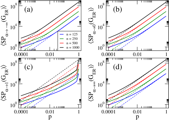
Figure 1: Average value of the Stolarsky–Puebla index $\left<SP_{\alpha}(G_{\mbox{\tiny ER}})\right>$ as a function of the probability $p$ of Erdös-Rényi networks of size $n$. Here (a) $\alpha\to-\infty$, (b) $\alpha\to 0$, (c) $\alpha\to 1$, and (d) $\alpha\to\infty$. Dashed lines correspond to Eq. (9).

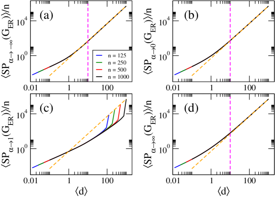
Figure 2: Average value of the Stolarsky–Puebla index $\left<SP_{\alpha}(G_{\mbox{\tiny ER}})\right>$, normalized to the network size $n$, as a function of the average degree $\left<d\right>$ of Erdös-Rényi networks. Same curves as in Fig. 1. Orange dashed lines are Eq. (11). The vertical magenta dashed lines indicate $\left<d\right>=10$.

From Eq. (9) we observe that $\left<SP_{\alpha}(G_{\mbox{\tiny ER}})\right>\propto nf[(n-1)p)]$ or

$$\left<SP_{\alpha}(G_{\mbox{\tiny ER}})\right>\propto nf(\left<d\right>).$$ (10)

Therefore, in Fig. 2 we plot again the average Stolarsky–Puebla indices reported in Fig. 1, but now normalized to $n$, as a function of $\left<d\right>$ showing that all indices are now properly scaled; i.e. the curves painted in different colors for different network sizes fall on top of each other. Moreover, we can rewrite Eq. (10) as

$$\frac{\left<SP_{\alpha}(G_{\mbox{\tiny ER}})\right>}{n}\approx\frac{1}{2}\left<d\right>^{2}.$$ (11)

In Fig. 2, we show that Eq. (11) (orange-dashed lines) indeed describe well the data (thick full curves) for $\left<d\right>\geq 10$; except for $\left<SP_{\alpha\to 1}(G_{\mbox{\tiny ER}})\right>$, see Fig. 2(c).

It is relevant to stress that even when Eq. (10) was expected to be valid in the dense limit (i.e. for $\left<d\right>\gg 1$), it is indeed valid for any $\left<d\right>$ as clearly seen in Fig. 2.

3.2 $SP_{\alpha}(G)$ on random geometric graphs

As in the previous Subsection, here we present the average values of selected Stolarsky–Puebla indices. Again, all averages are computed over ensembles of $10^{7}/n$ random graphs, each ensemble characterized by a fixed parameter pair $(n,r)$.

In Fig. 3 we present the average Stolarsky–Puebla index $\left<SP_{\alpha}(G_{\mbox{\tiny ER}})\right>$ for $\alpha\to-\infty$, $\alpha\to 0$, $\alpha\to 1$, and $\alpha\to\infty$ as a function of the connection radius $r$ of RG graphs of sizes $n=\{125,250,500,1000\}$. For comparison purposes, Fig. 3 is equivalent to Fig. 1. In fact, all the observations made in the previous Subsection for ER networks are also valid for RG graphs by just replacing $G_{\mbox{\tiny ER}}\to G_{\mbox{\tiny RG}}$ and $p\to g(r)$, with [23]

$$g(r)=\left\{\begin{array}[]{ll}r^{2}\left[\pi-\frac{8}{3}r+\frac{1}{2}r^{2}\right]&\quad 0\leq r\leq 1\,,\vspace{0.25cm}\\ \frac{1}{3}-2r^{2}\left[1-\arcsin(1/r)+\arccos(1/r)\right]+\frac{4}{3}(2r^{2}+1)\sqrt{r^{2}-1}-\frac{1}{2}r^{4}&\quad 1\leq r\leq\sqrt{2}\,.\end{array}\right.$$ (12)

As well as for ER networks, here, in the dense limit, when $nr\gg 1$, we can approximate $d_{u}\approx d_{v}\approx\left<d\right>$ with

$$\left<d\right>=(n-1)g(r).$$ (13)

Therefore, in the dense limit, $SP_{\alpha}(G_{\mbox{\tiny RG}})$ is well approximated by:

$$SP_{\alpha}(G_{\mbox{\tiny RG}})\approx\frac{1}{2}n\left[(n-1)g(r)\right]^{2}.$$ (14)

In Fig. 3, we show that Eq. (14) (dashed lines) indeed describes well the data (thick full curves) for large enough $r$; except for the case $\left<SP_{\alpha\to 1}(G_{\mbox{\tiny RG}})\right>$, see Fig. 3(c).

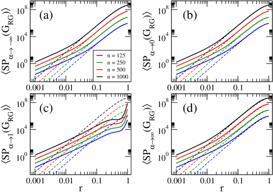
Figure 3: Average value of the Stolarsky–Puebla index $\left<SP_{\alpha}(G_{\mbox{\tiny RG}})\right>$ as a function of the connection radius $r$ of random geometric graphs of size $n$. Here (a) $\alpha\to-\infty$, (b) $\alpha\to 0$, (c) $\alpha\to 1$, and (d) $\alpha\to\infty$. Dashed lines correspond to Eq. (14).

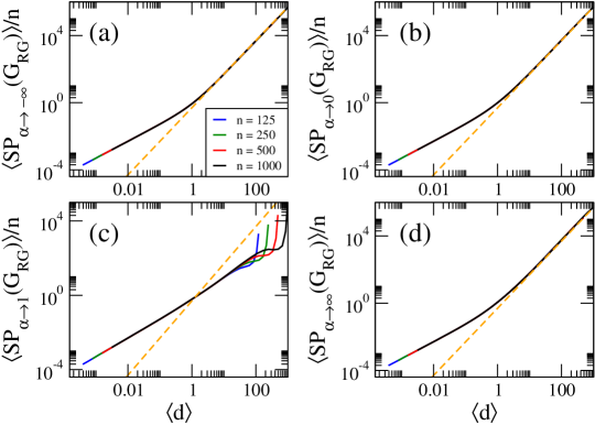
Figure 4: Average value of the Stolarsky–Puebla index $\left<SP_{\alpha}(G_{\mbox{\tiny GR}})\right>$, normalized to the network size $n$, as a function of the average degree $\left<d\right>$ of random geometric graphs. Same curves as in Fig. 3. Orange dashed lines are Eq. (15). The vertical magenta dashed lines indicate $\left<d\right>=10$.

It is quite remarkable to note that by substituting the average degree of Eq. (13) into Eq. (14) we get exactly the same expression of Eq. (11):

$$\frac{\left<SP_{\alpha}(G_{\mbox{\tiny RG}})\right>}{n}\approx\frac{1}{2}\left<d\right>^{2}.$$ (15)

So, in Fig. 4 we plot again the average Stolarsky–Puebla indices reported in Fig. 3 for RG graphs, but now normalized to $n$, as a function of $\left<d\right>$ showing that all curves are now properly scaled. Also, in Fig. 4, we show that Eq. (15) (orange-dashed lines) indeed describes well the data (thick full curves) for $\left<d\right>\geq 10$. We note that as well as for ER networks, here for RG graphs we do not observe the scaling of $\left<SP_{\alpha\to 1}(G_{\mbox{\tiny RG}})\right>$.

4   Discussion and conclusions

We have introduced a degree–based variable topological index inspired on the Stolarsky mean, known as the generalization of the logarithmic mean. We named this new index as the Stolarsky–Puebla index $SP_{\alpha}(G)$, see Eq. (6). For given values of $\alpha$, the Stolarsky–Puebla index is related to well-known topological indices, in particular it reproduces several mean Sombor indices $mSO_{\alpha}(G)$, see Eq. (7).

We want to add that the inequality of Eq. (4) can be straightforwardly used to state inequalities for the indices $SP_{\alpha}(G)$ and $mSO_{\alpha}(G)$, as well as for related indices:

$$SP_{-1}(G)=mSO_{\alpha\to 0}(G)\leq SP_{\alpha\to 0}(G)\leq mSO_{1/3}(G)\leq SP_{2}(G)=mSO_{1}(G)$$ (16)

or

$$R^{-1}(G)\leq\mbox{LogMean}(G)\leq mSO_{1/3}(G)\leq 2^{-1}M_{1}(G)\,,$$ (17)

which sets bounds for the logarithmic–mean topological index

$$\mbox{LogMean}(G)=\left\{\begin{array}[]{ll}d_{u}&\mbox{if $d_{u}=d_{v}$},\\ \displaystyle\frac{d_{u}-d_{v}}{\ln d_{u}-\ln d_{v}}&\mbox{otherwise},\end{array}\right.$$ (18)

with respect to the reciprocal Randic index, the mean Sombor index with $\alpha=1/3$, and the first Zagreb index.

Since there are not many degree–based topological indices including logarithmic functions (as well-known exceptions we can mention the logarithms of the three multiplicative Zagreb indices [7] and the Adriatic indices [24, 25]) we want to highlight the release of the logarithmic–mean topological index $\mbox{LogMean}(G)$ of Eq. (18) as well as the identric–mean index

$$\mbox{idLogMean}(G)=\left\{\begin{array}[]{ll}d_{u}&\mbox{if $d_{u}=d_{v}$},\\ \displaystyle\frac{d_{u}-d_{v}}{d_{u}\ln d_{u}-d_{v}\ln d_{v}}&\mbox{otherwise},\end{array}\right.$$ (19)

corresponding to $SP_{\alpha\to 0}(G)$ and $SP_{\alpha\to 1}(G)$, respectively.

We have also applied the Stolarsky–Puebla index $SP_{\alpha}(G)$ to Erdös-Rényi (ER) networks and random geometric (RG) graphs and within a statistical random matrix theory approach we demonstrated that $\left<SP_{\alpha}(G)\right>$, normalized to the order of the network, scales with the corresponding average degree $\left<d\right>$. However, it is fair to recognize that, for both random network models, $\left<SP_{\alpha\to 1}(G)\right>=\left<\mbox{idLogMean}(G)\right>$ did not scale; so we believe that the identric–mean index deserves further investigation.

In addition, from Eq. (16) we are able to write an equivalent inequality but for the corresponding average values:

$$\left<SP_{-1}(G)\right>\leq\left<\mbox{LogMean}(G)\right>\leq\left<mSO_{1/3}(G)\right>\leq\left<SP_{2}(G)\right>.$$ (20)

Indeed, we verified that (20) is satisfied for both, ER random networks and RG graphs (not shown here). Moreover, we computationally found that

$$\left<\mbox{idLogMean}(G)\right>\leq\left<SP_{\alpha\neq 1}(G)\right>,$$ (21)

for the two random network models we study here (not explicitelly shown here but partially observed in Figs. 1 and 3). The equalities in Eqs. (20) and (21) are attained when $p=1$ and $r=\sqrt{2}$, for ER random networks and RG graphs, respectively.

Finally, we want to recall that through a quantitative structure property relationship (QSPR) analysis it was shown [11] that $mSO_{\alpha\to\pm\infty}(G)$ are good predictors of the standard enthalpy of vaporization, the enthalpy of vaporization, and the heat of vaporization at 25^∘C of octane isomers. Furthermore, since $SP_{\alpha\to\pm\infty}(G)=mSO_{\alpha\to\pm\infty}(G)$, we can conclude that $SP_{\alpha\to\pm\infty}(G)$ correlate well with the aforementioned physicochemical properties of octane isomers.

In future works we plan to explore mathematical and computational properties of $SP_{\alpha}(G)$, as well as finding optimal bounds and new relationships with known topological indices.

References

• [1] K. B. Stolarsky, Generalizations of the logarithmic mean, Mathematics Magazine 48 (1975) 87–92.
• [2] T.-P. Lin, The power mean and the logarithmic mean, The American Mathematical Monthly 81 (1974) 879–883.
• [3] P. S. Bullen, Handbook of Means and Their Inequalities, Kluwer, Dordrecht, 2003.
• [4] S. Sykora, Mathematical means and averages: basic properties. 3. Stan’s Library, Castano Primo, Italy, 2009.
• [5] B. Ostle, H. L. Terwilliger, A comparison of two means, Proc. Montana Acad. Sci. 17 (1957) 69–70.
• [6] B. C. Carlson, Some inequalities for hypergeometric functions, Proc. Amer. Math. Soc. 17 (1966) 32–39.
• [7] I. Gutman, Degree–based topological indices, Croat. Chem. Acta 86 (2013) 351–361.
• [8] I. Gutman, B. Furtula, C. Elphick, Three new/old vertex–degree–based topological indices, MATCH Commun. Math. Comput. Chem. 72 (2014) 617–632.
• [9] V. R. Kulli, The $(a,b)-KA$ indices of polycyclic aromatic hydrocarbons and benzenoid systems, Int. J. Math. Trends Tech. 65 (2019) 115–120.
• [10] I. Gutman, N. Trinajstić, Graph theory and molecular orbitals. Total $\pi$-electron energy of alternant hydrocarbons, Chem. Phys. Lett. 17 (1972) 535–538.
• [11] R. Aguilar-Sanchez, J. A. Mendez-Bermudez, E. D. Molina, J. M. Rodriguez, J. M. Sigarreta, A survey on Sombor indices: An overview over recent and new results, to be submitted (2021).
• [12] R. Solomonoff, A. Rapoport, Connectivity of random nets, Bull. Math. Biophys. 13 (1951) 107–117.
• [13] P. Erdös, A. Rényi, On random graphs, Publ. Math. (Debrecen) 6 (1959) 290–297.
• [14] P. Erdös, A. Rényi, On the evolution of random graphs, Inst. of the Hung. Acad. of Sci. 5 (1960) 17–61.
• [15] P. Erdös, A. Rényi, On the strength of connectedness of a random graph, Acta Mathematica Hungarica 12 (1961) 261–267.
• [16] J. Dall, M. Christensen, Random geometric graphs, Phys. Rev. E 66 (2002) 016121.
• [17] M. Penrose, Random Geometric Graphs, Oxford University Press, Oxford, 2003.
• [18] C. T. Martinez-Martinez, J. A. Mendez-Bermudez, J. M. Rodriguez, J. M. Sigarreta, Computational and analytical studies of the Randić index in Erdös–Rényi models, Appl. Math. Comput. 377 (2020) 125137.
• [19] R. Aguilar-Sanchez, I. F. Herrera-Gonzalez, J. A. Mendez-Bermudez, J. M. Sigarreta, Computational properties of general indices on random networks, Symmetry 12 (2020) 1341.
• [20] C. T. Martinez-Martinez, J. A. Mendez-Bermudez, J. M. Rodriguez, J. M. Sigarreta, Computational and analytical studies of the harmonic index in Erdös–Rényi models, MATCH Commun. Math. Comput. Chem. 85 (2021) 395–426.
• [21] R. Aguilar-Sanchez, J. A. Mendez-Bermudez, F. A. Rodrigues, J. M. Sigarreta-Almira, Topological versus spectral properties of random geometric graphs, Phys. Rev. E 102 (2020) 042306.
• [22] R. Aguilar-Sanchez, J. A. Mendez-Bermudez, J. M. Rodriguez, J. M. Sigarreta, Normalized Sombor indices as complexity measures of random networks, Entropy 23 (2021) 976.
• [23] E. Estrada, M. Sheerin, Random rectangular graphs, Phys Rev. E 91 (2015) 042805.
• [24] D. Vukicevic, Bond additive modeling 2. Mathematical properties of max-min Rodeg index, Croat. Chem. Acta 83 (2010) 261–273.
• [25] D. Vukicevic, Bond additive modeling 5. Mathematical properties of the variable sum Exdeg index, Croat. Chem. Acta 84 (2011) 93–101.