appendixReferences
More powerful selective inference
for the graph fused lasso
Abstract
The graph fused lasso — which includes as a special case the one-dimensional fused lasso — is widely used to reconstruct signals that are piecewise constant on a graph, meaning that nodes connected by an edge tend to have identical values. We consider testing for a difference in the means of two connected components estimated using the graph fused lasso. A naive procedure such as a z-test for a difference in means will not control the selective Type I error, since the hypothesis that we are testing is itself a function of the data. In this work, we propose a new test for this task that controls the selective Type I error, and conditions on less information than existing approaches, leading to substantially higher power. We illustrate our approach in simulation and on datasets of drug overdose death rates and teenage birth rates in the contiguous United States. Our approach yields more discoveries on both datasets.
Keywords: Post-selection inference, Penalized Regression, Piecewise constant, Hypothesis testing, Changepoint Detection
1 Introduction
We consider a vector , assumed to be a noisy realization of a signal ,
| (1) |
with known variance . We assume that has some underlying structure of interest. For instance, might be sparse, with few non-zero elements, or piecewise constant, meaning that the elements of are ordered, and adjacent elements tend to take on equal values.
It is natural to estimate by solving the optimization problem
| (2) |
where is an penalty matrix that encodes the structure of . Problem (2) is a special case of the generalized lasso with an identity design matrix [Tibshirani and Taylor,, 2011, Hastie et al.,, 2015, Arnold and Tibshirani,, 2016]. While the ideas in this paper apply for a general design matrix, we make use of an identity design matrix to simplify the discussion. Many well-known regression problems involving penalties can be viewed as special cases of the generalized lasso; examples include the lasso [Tibshirani,, 1996], the fused lasso signal approximator [Tibshirani et al.,, 2005, Friedman et al.,, 2007, Rinaldo,, 2009], the graph fused lasso [Tibshirani and Taylor,, 2011, Hastie et al.,, 2015], and trend filtering [Kim et al.,, 2009, Tibshirani,, 2014].
Despite the abundant literature on algorithms for computing in (2) [Johnson,, 2013, Tibshirani and Taylor,, 2011, Xin et al.,, 2014, Ramdas and Tibshirani,, 2016, Zhu,, 2017, Arnold and Tibshirani,, 2016, Friedman et al.,, 2007] and on its theoretical properties [Sadhanala et al.,, 2016, Tibshirani and Taylor,, 2011, Rinaldo,, 2009, Harchaoui and Lévy-Leduc,, 2010], the topic of inference for the generalized lasso remains less developed. In this work, we focus on testing a null hypothesis that was determined after observing in (2).
More precisely, suppose that we perform the graph fused lasso, a special case of (2),
| (3) |
where is an undirected graph, , and indicates that the th and th vertices in the graph are connected by an edge [Tibshirani and Taylor,, 2011]. For sufficiently large values of the non-negative tuning parameter , we will have for some . We can segment into connected components — that is, sets of elements of that are connected in the original graph and share a common value. We might then consider testing the null hypothesis that the true mean of is the same across two estimated connected components, i.e.,
| (4) |
where and are connected components of , with cardinality and , and . This is equivalent to testing versus , where
| (5) |
Here, is chosen based on the data, i.e., we selected the contrast vector in (5) because and are estimated connected components. We focus on developing a test of that controls the selective Type I error rate [Fithian et al.,, 2014], i.e., one for which the probability of rejecting at level , given that holds and we decided to test , is no greater than :
| (6) |
It is not hard to see that a standard two-sample z-test of , with -value , fails to account for the fact that we decided to test after looking at the data, and therefore does not control the selective Type I error rate (6). To address this problem, Hyun et al., [2018] propose an elegant approach for testing that makes use of the selective inference framework developed by Lee et al., [2016], Fithian et al., [2014], and Tibshirani et al., [2016]. Their key insight is as follows: the set of that yields a particular output for the first steps of the dual path algorithm for solving (2) is a polyhedron, of the form , for a matrix that can be explicitly computed. Thus, conditional on belonging to this polyhedral set, the linear contrast follows a truncated normal distribution, with parameters that are a function of , , and , for any that is based on the output of (2). It is thus possible to compute valid -values for the null hypothesis in (4) in the sense of (6), by conditioning on the outputs from the first steps of the dual path algorithm.
Our paper relies on a simple observation: the proposal considered in Hyun et al., [2018] involves conditioning on much more information than is used to construct the contrast vector in (5). As pointed out by Fithian et al., [2014] and Liu et al., [2018], conditioning on unnecessary information leads to reduced power. In this paper, we make use of recent ideas from Jewell et al., [2022] to develop a computationally-efficient test of that conditions on substantially less information than Hyun et al., [2018], thereby obtaining much higher power while still guaranteeing valid inference in the sense of (6).
While this paper was in preparation, Le Duy and Takeuchi, [2021] independently developed a test of that has higher power than Hyun et al., [2018]. Compared to that paper, our proposal (i) conditions on less unnecessary information; (ii) enjoys better numerical stability; and (iii) leads to more interpretable -values. Details are provided in Appendix A.13.
The rest of this paper is organized as follows. In Section 2, we briefly review the dual path algorithm for solving (2), and the existing proposals for selective inference for this problem. In Section 3, we introduce our selective inference procedure, which provides a computationally-efficient approach to condition on less information than Hyun et al., [2018]. Section 4 outlines some extensions, and Section 5 compares the performance of our proposal to that of Hyun et al., [2018] in simulation. A real data application is in Section 6, and a discussion of future work is in Section 7. Proofs and other technical details are relegated to the Appendix.
Throughout this paper, we will use the following notational conventions. The th row of a matrix is denoted . Given a set of positive integers, is the submatrix with rows in , is the submatrix with rows not in , and is the cardinality of the set . For a vector , and denote its and norms, respectively. In addition, denotes the projection matrix onto the orthogonal complement of , i.e., , where is the -dimensional identity matrix. We use to denote the indicator function. For a positive integer , we define .
2 Background on the generalized lasso
In this section, we review the selective inference framework of Hyun et al., [2018] for testing hypotheses based upon the generalized lasso estimator (2), which includes the graph fused lasso as a special case. Their framework relies on the dual path algorithm of Tibshirani and Taylor, [2011] for solving (2). Thus, we begin with a very brief overview of that algorithm.
2.1 The dual problem, and the dual path algorithm
Tibshirani and Taylor, [2011] develop an efficient path algorithm for solving the dual problem for (2), which takes the form
| (7) |
and is related to (2) through the identity , where the notation and makes explicit that and are functions of . This dual path algorithm is detailed in Appendix A.1. While the details of the algorithm are not important for the current paper, we briefly summarize the main idea. The algorithm begins with , and then proceeds through a series of steps, corresponding to decreasing values of . The th step involves computing a boundary set , which consists of the subset of indices of the vector for which the inequality constraint in (7) is tight. The signs of the elements of associated with this boundary set, , are also computed. These quantities satisfy
| (8) |
for a range of values corresponding to the th step [Tibshirani and Taylor,, 2011]. In (8), and correspond to the submatrices of with rows in and not in , respectively, and is the projection matrix onto the null space of . To summarize, (8) indicates that can be computed from , for an appropriate range of values.
The next proposition considers the special case of the graph fused lasso problem (3).
Proposition 1.
Let denote the boundary set that results from the th step of the dual path algorithm for (3), and let denote the solution to (3). Let denote the subgraph of with edges in the boundary set removed, and let denote the connected components of . Then, under (1), with probability 1, if and only if for some .
2.2 Existing work on selective inference for the generalized lasso
The main idea behind selective inference is as follows: when testing a null hypothesis that is a function of the data, to control the selective Type I error in the sense of (6), we must condition on the information used to construct that null hypothesis [Tibshirani et al.,, 2016, Lee et al.,, 2016, Fithian et al.,, 2014]. In particular, to test a null hypothesis of the form where is a function of the data, we must condition on the information used to construct .
In a recent elegant line of work, a number of authors have shown that the model selection events of several well-known model selection procedures, including the lasso [Lee et al.,, 2016], stepwise regression [Loftus and Taylor,, 2014, Tibshirani et al.,, 2016], and marginal screening [Reid et al.,, 2017], can be written as polyhedral constraints on . More precisely, conditioning on the selected model (and in some cases, additional information) is equivalent to conditioning on a polyhedral set , where the matrix and the vector can be explicitly computed. Thus, we can test null hypotheses that are a function of the selected model by considering the null distribution of truncated to a polyhedral set.
Recently, Hyun et al., [2018] extended this line of work to develop an approach for selective inference for the generalized lasso (2). Their key insight is as follows:
The set of that leads to a specified output for the first steps of the dual path algorithm for (2) is a polyhedron, i.e., , for a matrix that can be explicitly computed.
Proposition 2 details this result.
Proposition 2 (Proposition 3.1 in Hyun et al., [2018]).
Consider solving (2) using the dual path algorithm for . For the th step, , define
| (9) |
where the boundary set and the sign vector of the boundary set are defined in Algorithm 1 (see Appendix A.1), and and for , and specified in Algorithm 1.
Then the set is of the form for some matrix that can be constructed explicitly based on .
Motivated by this result, Hyun et al., [2018] proposed to test , where is a function of the generalized lasso estimator, via a -value of the form
| (10) |
In (10), conditioning on eliminates the nuisance parameter ; see Section 3.1 of Fithian et al., [2014]. Now, under (1), the conditional distribution of is normal with mean zero and variance , truncated to a set that can be characterized and efficiently computed using Proposition 2. This yields the -value in (10). Furthermore, unlike the z-test based on the naive -value , a test that rejects when the -value in (10) is less than some level controls the selective Type I error rate, in the sense of (6).
We emphasize that the -value in (10) conditions on the event ; that is, on all of the outputs of the first steps of the dual path algorithm (rather than simply the th step). However, typically the contrast vector in is constructed using only (at most) the output of the th step in the dual path algorithm. In what follows, we will consider conditioning on much less information than (10). This will result in a test that controls the selective Type I error as in (6), and that has substantially higher power under the alternative.
3 Proposed approach
3.1 What should we condition on?
To control the selective Type I error in (6), we must condition on the aspect of the data that led us to test the specific null hypothesis [Fithian et al.,, 2014, Hyun et al.,, 2018].
If a data analyst wishes to choose the contrast vector in the null hypothesis by inspecting the elements of resulting from the th step of the dual algorithm of the generalized lasso problem (2), then there is no reason to condition on (as was done by Hyun et al., [2018]), since the outputs of the first steps of the dual path algorithm are not considered in constructing . In fact, according to (8), which states that and uniquely determine , the data analyst need only condition on and , rather than on .
Furthermore, the data analyst might construct the contrast vector in to take on a constant value within each connected component of , as in (4) and (5). Recall from Proposition 1 that the connected components of are equivalent to the connected components of the subgraph . Therefore, it suffices to condition only on the connected components of the subgraph , or even on just the pair of connected components under investigation in (4).
What is the disadvantage of conditioning on , as in Hyun et al., [2018]? Conditioning on too much information leads to a loss of power [Fithian et al.,, 2014, Liu et al.,, 2018, Lee et al.,, 2016, Jewell et al.,, 2022]. We wish to condition on less information to achieve higher power than Hyun et al., [2018], while controlling the selective Type I error (6). Of course, this could result in computational challenges, as the conditioning sets described in the use cases above are not polyhedral, so the conditional distribution of is no longer a normal truncated to an easily-characterized set.
In what follows, we focus on the case where the data analyst constructs the contrast vector to take on a constant value in each connected component of , and consider a -value of the form
| (11) |
In (11), and are two connected components estimated from the data realization and used to construct the contrast vector in (5), and is the set of connected components obtained from applying steps of the dual path algorithm for (3) to the random variable . Roughly speaking, this -value answers the following question:
Assuming that there is no difference between the population means of and , then what’s the probability of observing such a large difference in the sample means of and , given that these two connected components were estimated from the data?
While our proposed -value conditions on far less information than Hyun et al., [2018], the recent proposal of Le Duy and Takeuchi, [2021] takes an intermediate approach. They condition on the full boundary set at the th step of the dual path algorithm (and thus, implicitly, on all of the connected components in ), whereas we condition only on the two connected components of interest. See Appendix A.13 for further discussion and comparison.
3.2 Illustrative example
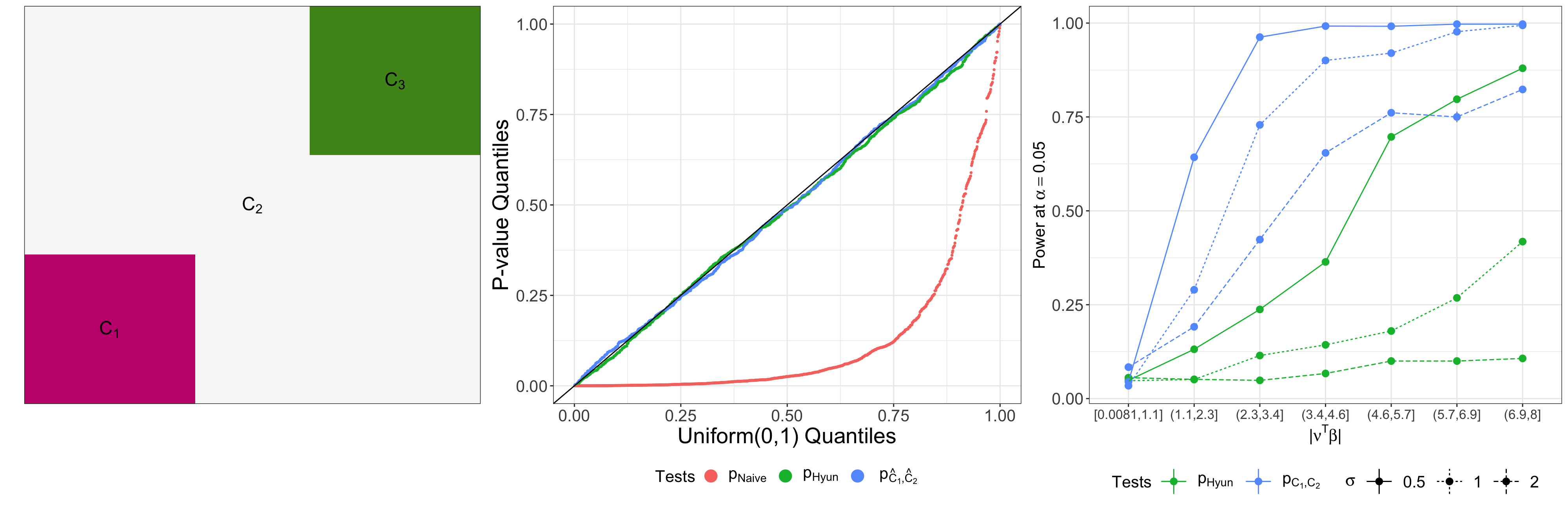
We now demonstrate that conditioning on less information leads to increased power, using an example involving the graph fused lasso applied to a two-dimensional grid graph.
| 0.63 | ||
| 0.25 | ||
| 0.17 |
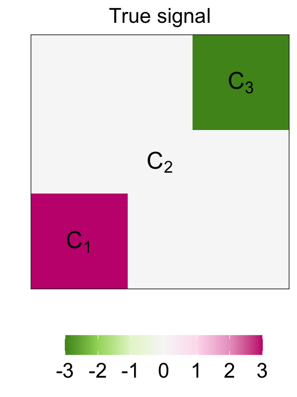
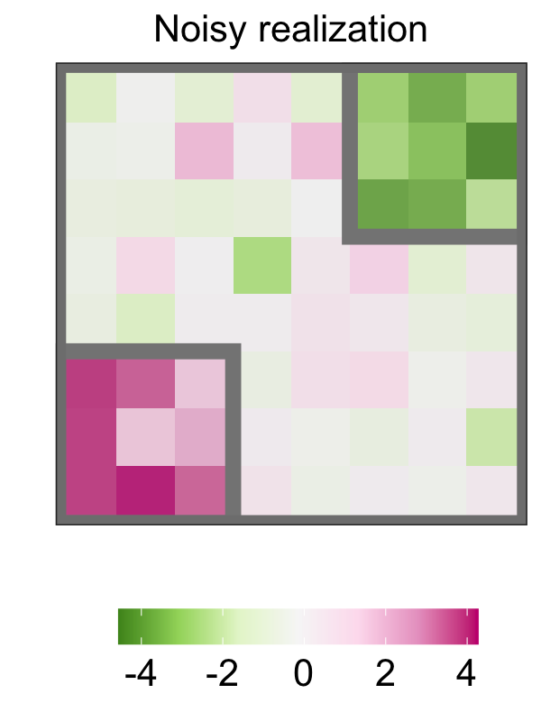
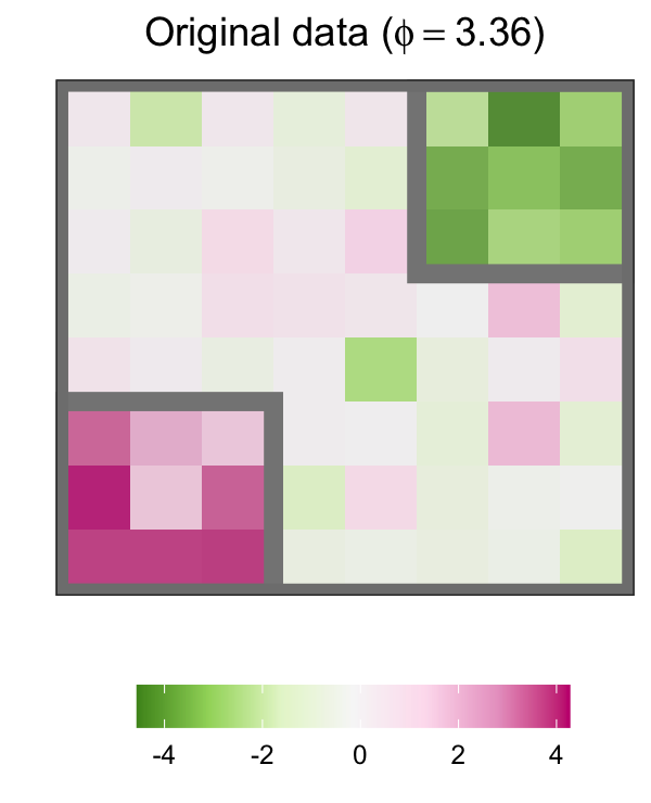
To begin, we constructed a graph composed of nodes arranged in an grid, such that each node is connected to its four closest (up, down, left, right) neighbors. We generated data on this grid according to (1), where has three piecewise constant segments, , , and , with means of , , and , respectively. The true values of , as well as the data generated from this model, are shown in Figures 1(a)–(b). On this particular data set, steps of the dual path algorithm for the graph fused lasso recovered the true connected components exactly.
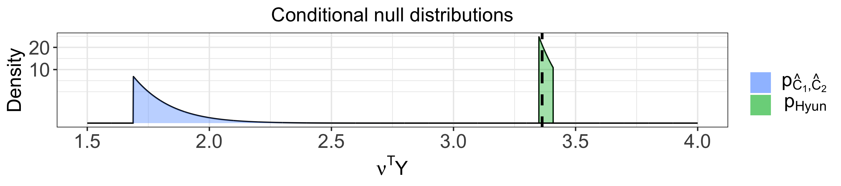
For each pair of connected components, we then constructed a contrast vector as in (4), so that posits that the two components being tested have the same mean. We tested using the -values and given in (10) and (11), respectively. The -values for all pairs of connected components are displayed in Figure 1(c). Because conditions on unnecessary information, the test based on has extremely low power and it cannot reject any . By contrast, the test based on has higher power. In Figure 1(d), we display the null distribution of , conditional on the conditioning sets in (10) and (11).
3.3 Properties of
The following result establishes key properties of in (11).
Proposition 3.
Suppose that . Define
| (12) |
Let . Then, under ,
| (13) |
Moreover, the test that rejects if controls the selective Type I error.
Therefore, to compute the -value in (11), it suffices to characterize the set
| (14) |
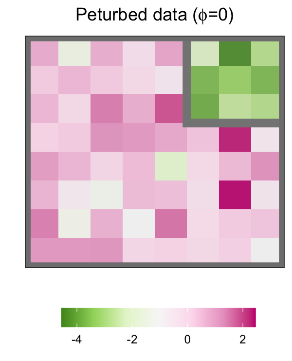
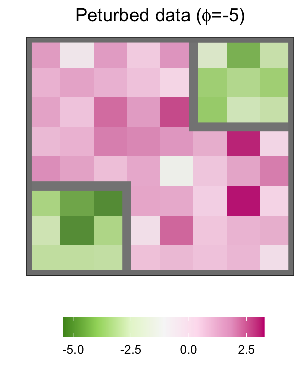
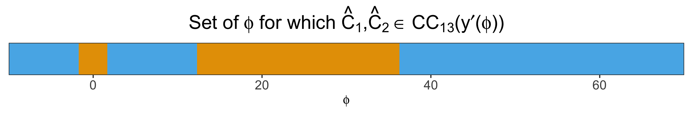
We can think of in (12) as a perturbation of the data by a function of along the direction defined by . Figure 2 illustrates this intuition in the toy example from Figure 1, in the context of a test for the difference in the means of and (see Figure 2(a)). Panel (a) displays the observed data, for which , where is defined in (5). In panel (b), we perturb the observed data to . Now the graph fused lasso with no longer detects the three connected components. In panel (c), we perturb the observed data to ; in this case, the graph fused lasso with estimates all three connected components. Therefore, and are in the set , but is not. Panel (d) displays .
We now leverage ideas from Jewell et al., [2022] to develop an efficient approach to compute the set (14). First, we characterize the set in (14) in Proposition 4. Recall that is the output of the th step of Algorithm 1. We first present a corollary of Proposition 2.
Corollary 1.
The set is an interval.
Proposition 4.
Let be the set of possible outputs of Algorithm 1 that yield and and can be obtained via a perturbation of defined in (12), i.e.,
| (15) |
Then, there exists an index set and scalars such that
-
1.
the set in (14) is the union of intervals:
(16) -
2.
(i.e., the sets and have the same cardinality); and
-
3.
, such that .
In words, Proposition 4 states that the set in (14) can be expressed as a union of intervals, each of which can be computed by applying Corollary 1 on a perturbation of . Next, we use Proposition 4 to develop an efficient recipe to compute by constructing the index set and scalars . To begin, we run the first steps of the dual path algorithm on the data . We then apply Corollary 1 to obtain the set . By construction, , because and are connected components estimated from the data . Therefore, we initialize the index set as . Then, for a small , we apply Corollary 1 to obtain the interval . If the left endpoint of this interval does not equal , then we must repeat with a smaller value of until we obtain an interval of the form . We can then check whether : if so, then and we update to include . Otherwise, remains unchanged. We continue in this vein, along the positive real line, until we reach an interval for which the right endpoint equals .
Finally, we proceed along the negative real line: we apply Corollary 1 to compute the interval . If , then is set to ; otherwise, remains unchanged. We iterate until the algorithm outputs an interval for which the left endpoint equals . Finally, . The procedure is summarized in Algorithm 2 of Appendix A.3.
In our implementation, we initialize with , which proves to be an efficient choice in experiments in Section 5 (see details in Appendix A.3). In principle, the running time of Algorithm 2 can be quite slow, and potentially even exponential in . However, in practice, the runtime of Algorithm 2 is nowhere near the worst-case upper bound (see Appendix A.11 for a detailed empirical study of the timing complexity of Algorithm 2). In addition, in Proposition 5, we describe an “early stopping” rule that guarantees a conservative -value and only requires running Algorithm 2 until we reach intervals containing and for some , as opposed to and . Then, the set is appended with and . This “early stopping” rule also applies to the extensions in Section 4.
Proposition 5.
Provided that , for any , we have that
| (17) |
where .
4 Extensions
4.1 Confidence intervals for
We now construct a confidence interval for , the difference between the population means of two connected components and resulting from the graph fused lasso.
Proposition 6.
Suppose that (1) holds, and let and be two connected components obtained from performing steps of the dual path algorithm for the graph fused lasso (3). For a given value of , define functions and such that
| (18) |
where is the cumulative distribution function of a random variable, truncated to the set defined in (14). Then has selective coverage [Lee et al.,, 2016, Fithian et al.,, 2014, Tibshirani et al.,, 2016] for , in the sense that
| (19) |
4.2 An alternative conditioning set
The conditioning set for involves the connected components of the graph fused lasso solution after steps of the dual path algorithm. However, in practice, a data analyst might prefer a more “user-facing” choice of , such as the value that yields connected components in the solution .
For this reason, we now consider a slight modification of ,
| (20) |
where the subscript on has been dropped, indicating that the number of steps of the graph fused lasso algorithm is no longer fixed; instead, the function now represents the graph fused lasso estimator tuned to yield exactly connected components. Thus, in , we condition on datasets for which are among connected components estimated using the graph fused lasso. It is not hard to show that Proposition 4 and Algorithm 2 require only minor modifications to enable the computation of the -values ; details are provided in Section A.8 of the Appendix.
5 Simulation study
We consider testing the null hypothesis , where, unless otherwise stated, is defined in (5) for a randomly-chosen pair of estimated connected components , of the solution to (3). We consider three -values: in (10), in (11), and the naive -value
| (21) |
and compare the selective Type I error (6) and power of the tests that reject when these -values are less than .
In the simulations that follow, comparing the power of the tests requires a bit of care. Because the null hypothesis involves the contrast vector , which is a function of the data, the effect size may differ across simulated datasets from the same data-generating distribution. Therefore, in what follows, we consider the power as a function of . Alternatively, we can separately assess the detection probability (i.e., the probability that and are true piecewise constant segments) and the “conditional power” [Hyun et al.,, 2021, Gao et al.,, 2020] (i.e., the probability of rejecting , given that , are true piecewise constant segments). Details are in Appendix A.9.
5.1 One-dimensional fused lasso
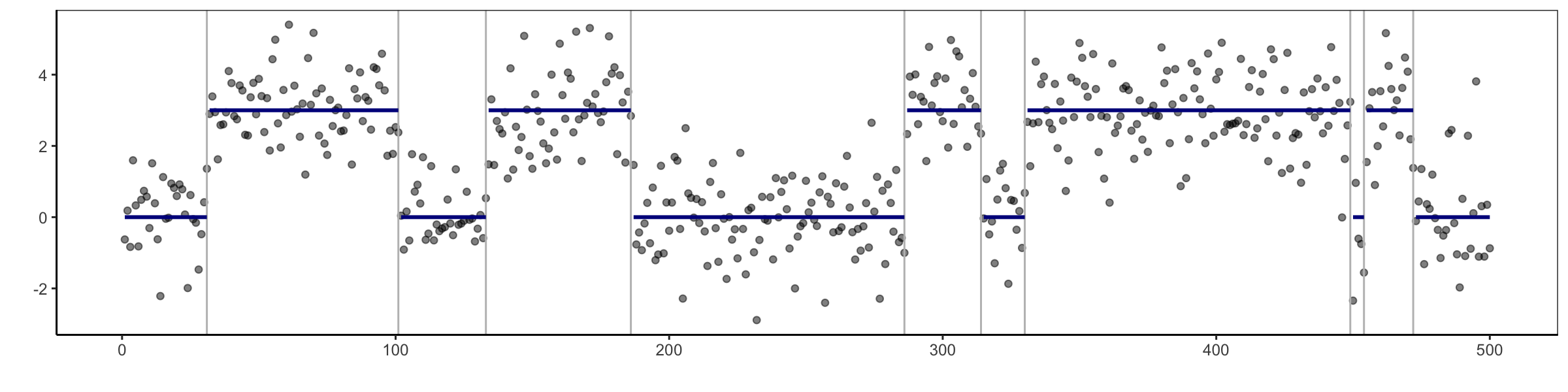
We first consider the special case of the graph fused lasso on a chain graph, in which the observations are ordered, and there is an edge between each pair of adjacent observations. This leads to the one-dimensional fused lasso problem [Tibshirani and Taylor,, 2011]. We simulated from the “middle mutation” model of Hyun et al., [2021], where the signal contains two true changepoints of size , and in turn, three connected components:
| (22) |
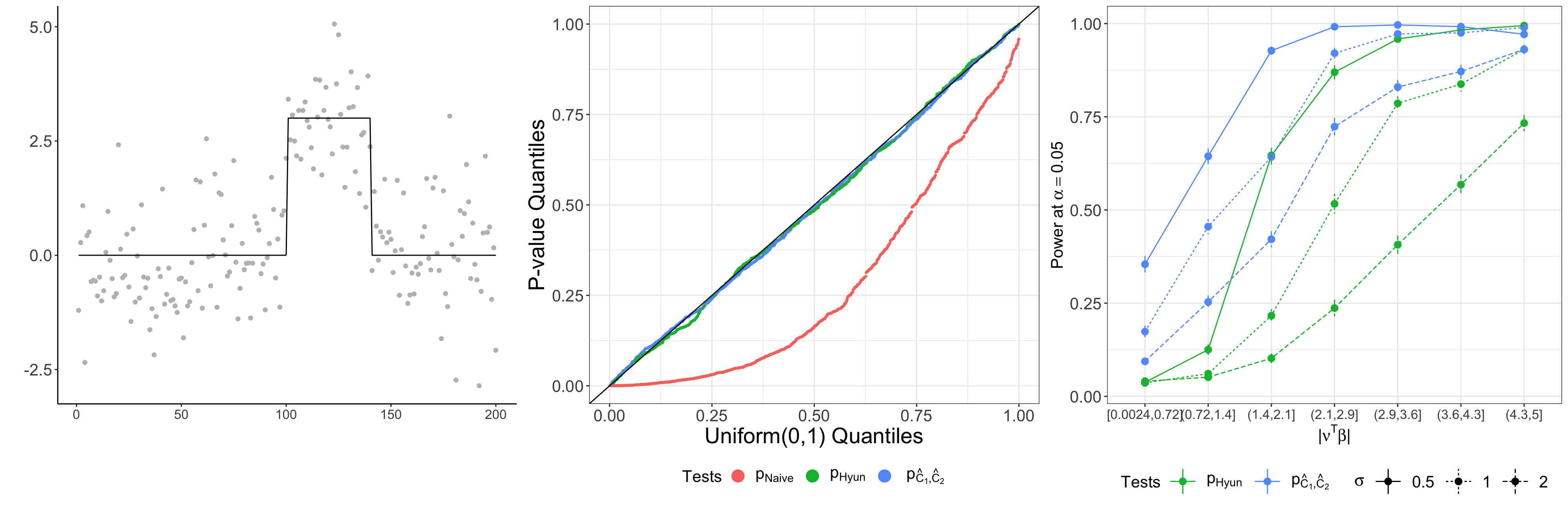
Figure 3(a) displays an example of this synthetic data with and .
5.1.1 Selective Type I error control under the global null
We simulated according to (22) with and . Therefore, the null hypothesis holds for all contrast vectors in , regardless of the pair of estimated connected components under consideration.
We solved (3) with steps in the dual path algorithm, which yields exactly three estimated connected components by the properties of the one-dimensional fused lasso. Then, for each simulated dataset, we computed in (11), in (10), and the naive -value in (21).
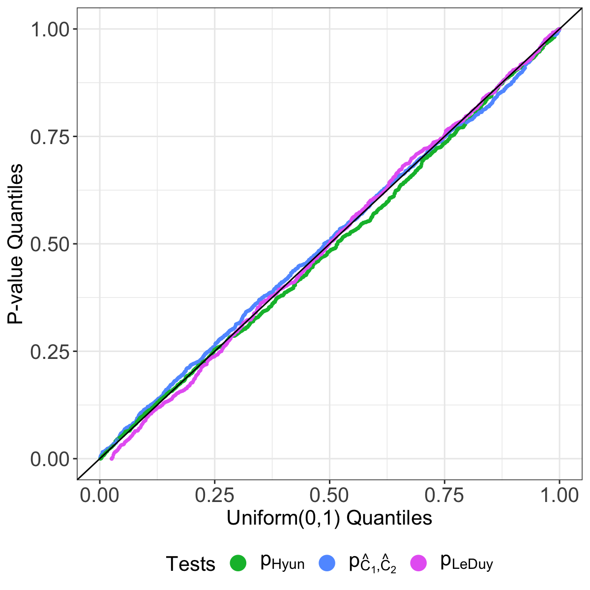
Figure 3(b) displays the observed -value quantiles versus Uniform quantiles, aggregated over 1,000 simulated datasets. We see that (i) the test based on the naive -value in (21), which does not account for the fact that the connected components were estimated from the data, is anti-conservative; and (ii) tests based on and control the selective Type I error (6).
5.1.2 Power as a function of effect size
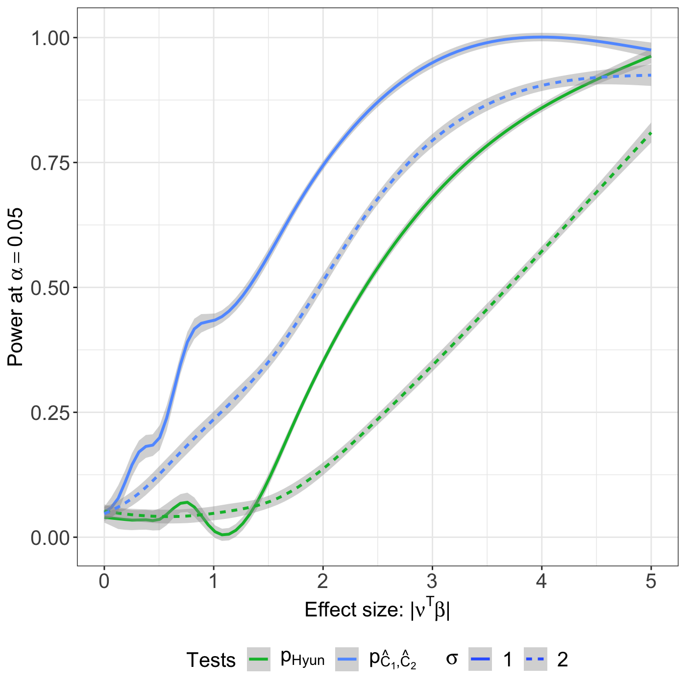
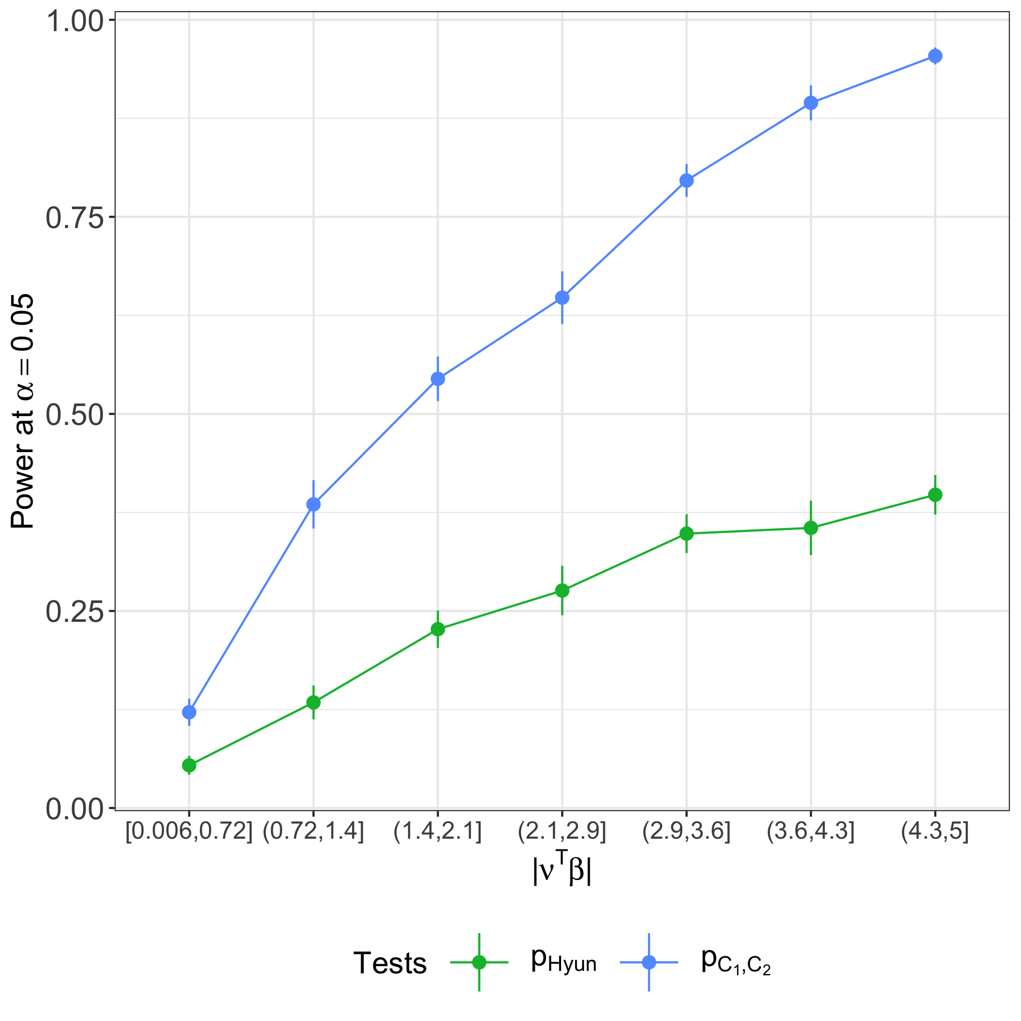
Next, we show that the test based on has higher power than that based on . We generated 1,500 datasets from (22) with , for each of ten evenly-spaced values of . For every simulated dataset, we solved (3) with . We then rejected if or was less than . Recalling that in (5) is a function of the data, and the effect size will vary across simulated datasets drawn from an identical distribution, we created seven evenly-spaced bins of the observed values of , and then computed the proportion of simulated datasets for which we rejected within each bin.
Results are in Figure 3(c). The power of each test increases as the value of increases. For a given bin of , the test based on has higher power than the test based on . For a given test and bin of , a smaller value of results in higher power. As an alternative to binning, we can use regression splines to estimate the power as a smooth function of the effect size; see Appendix A.9.
(a) (b) (c)
5.2 Two-dimensional fused lasso
We consider the graph fused lasso on a grid graph, constructed by connecting each node to its four closest neighbors (up, down, left, right). This leads to the two-dimensional fused lasso problem, also known as total-variation denoising [Tibshirani and Taylor,, 2011, Rudin et al.,, 1992].
The signal consists of with 64 observations arranged in an grid. It has three piecewise constant segments with means , 0, and , displayed in Figure 4(a):
| (23) |
5.2.1 Selective Type I error control under the global null
We simulated according to (23) with and . Thus, the null hypothesis holds for any contrast vector under consideration.
For each simulated dataset, we solved (3) with steps in the dual path algorithm, which typically yields between 2 and 4 estimated connected components. Then, provided that there was more than one connected component in the solution , we computed in (21), in (10), and in (11). We rejected if the -values are less than .
5.2.2 Power as a function of effect size
We generated data according to (23) with each of eight evenly-spaced values of and . For each simulated dataset, we solved (3) with steps in the dual path algorithm. Provided that there were at least two estimated connected components, we then computed in (10) and in (11), and rejected if the -values were less than .
In Figure 4(c), we display the proportion of simulated datasets for which we rejected using the two tests, over seven evenly-spaced bins of . For a given bin, the test based on has substantially higher power than that based on ; the power of each test increases as decreases.
(a) (b) (c)
5.2.3 Allowing for unknown variance
6 Data applications
In this section, we apply our proposed -value to a dataset consisting of two measures: (i) drug overdose death rates (deaths per 100,000 persons), and (ii) teenage birth rates (births per 1,000 females aged 15–19), in each of the 48 contiguous states in the United States [Centers for Disease Control and Prevention, 2020a, , Centers for Disease Control and Prevention, 2020b, ]. In what follows, we consider the two measures after applying a log transformation. We can think of the data as noisy measurements of the true drug overdose death and teenage birth rate rates in each state, which are known to exhibit geographic trends [Schieber et al.,, 2019, Ventura et al.,, 2014, Amin et al.,, 2017]. Therefore, we solve the graph fused lasso in (3) with a custom graph that encodes the geography of the 48 states: each state is a node, and there is an edge between each contiguous pair of states. We then consider testing the equality of measures for pairs of estimated connected components.
For each pair of connected components, we computed three -values: in (11), in (10), and in (21). We also computed confidence intervals for , the difference between population means of a pair of estimated connected components, using and , as described in Section 4.1, along with the naive confidence interval , where is the th quantile of the standard normal distribution. For each -value and confidence interval, we used to estimate in (1), where are the estimated connected components.
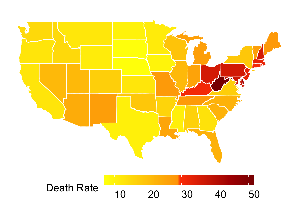
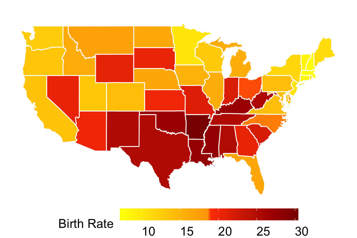
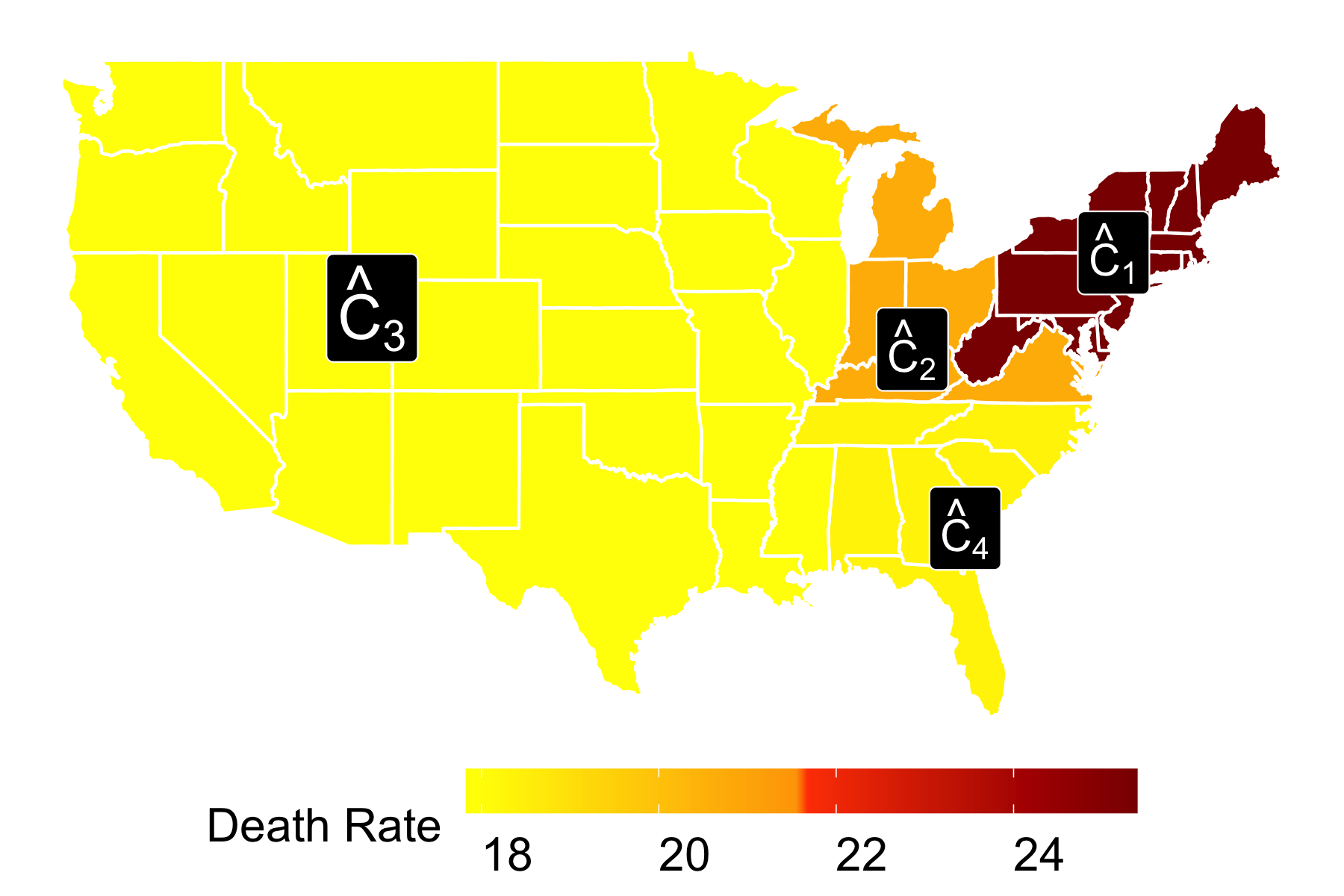
6.1 Drug overdose death rates in the contiguous U.S. in 2018
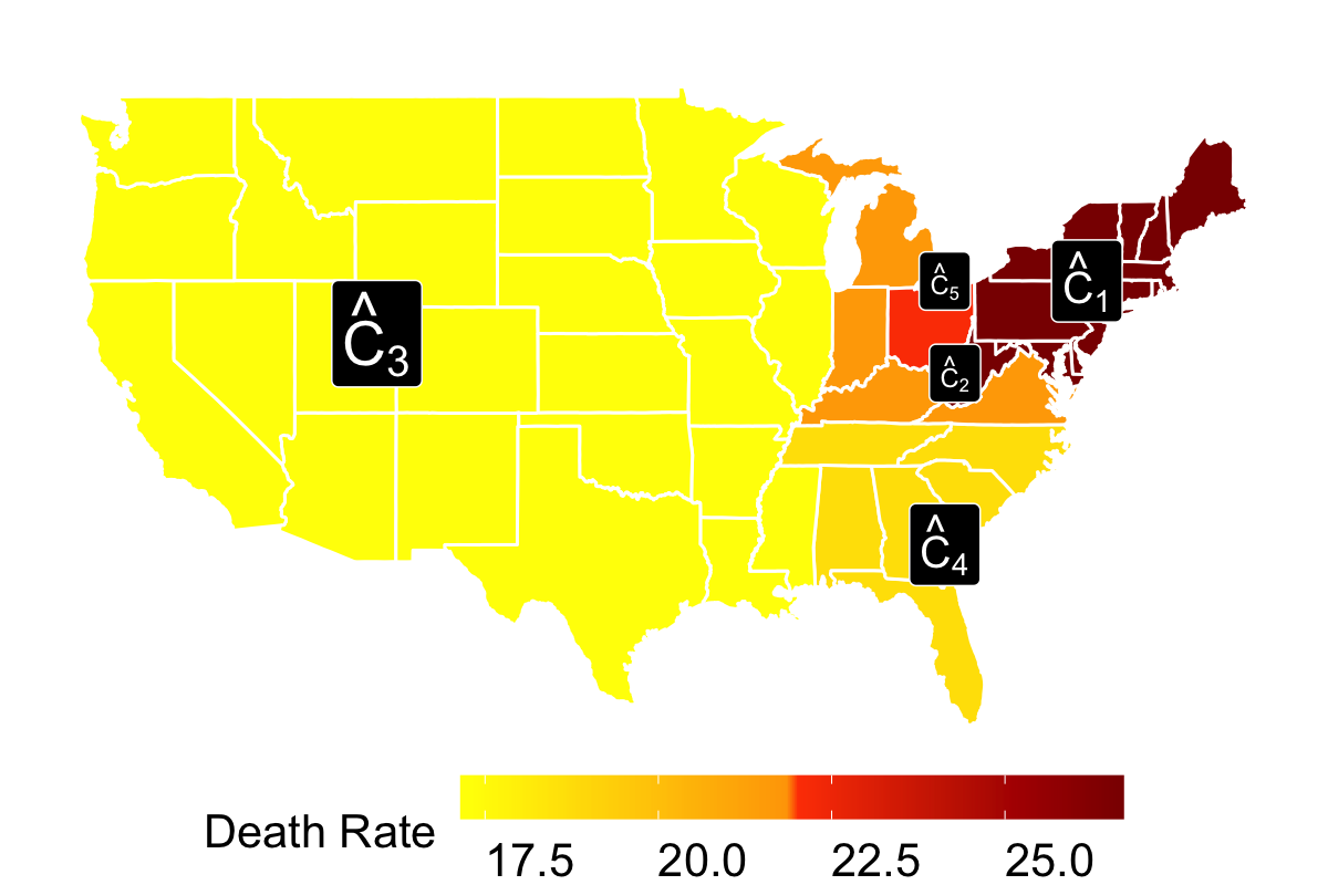
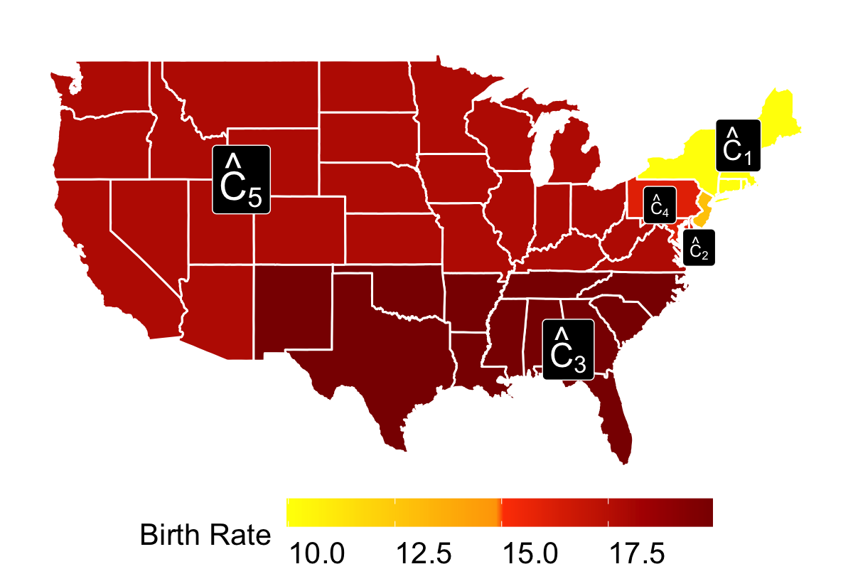
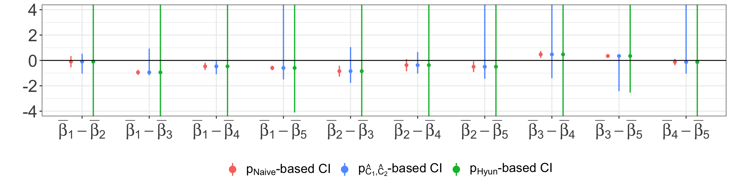
Figure 5(a) displays the drug overdose death rate in a color map. We solved (3) with steps in the dual path algorithm, which resulted in five connected components (see Appendix A.12 for results with other choices of ); the results are displayed in Figure 5(b). We have estimated a constant drug overdose death rate in five geographical regions, which we refer to as the Northeast (), Ohio (), the West and Mountain region (), the Southeast (), and the Midwest (). Among these regions, the Northeast and Midwest have the highest estimated drug overdose rates.
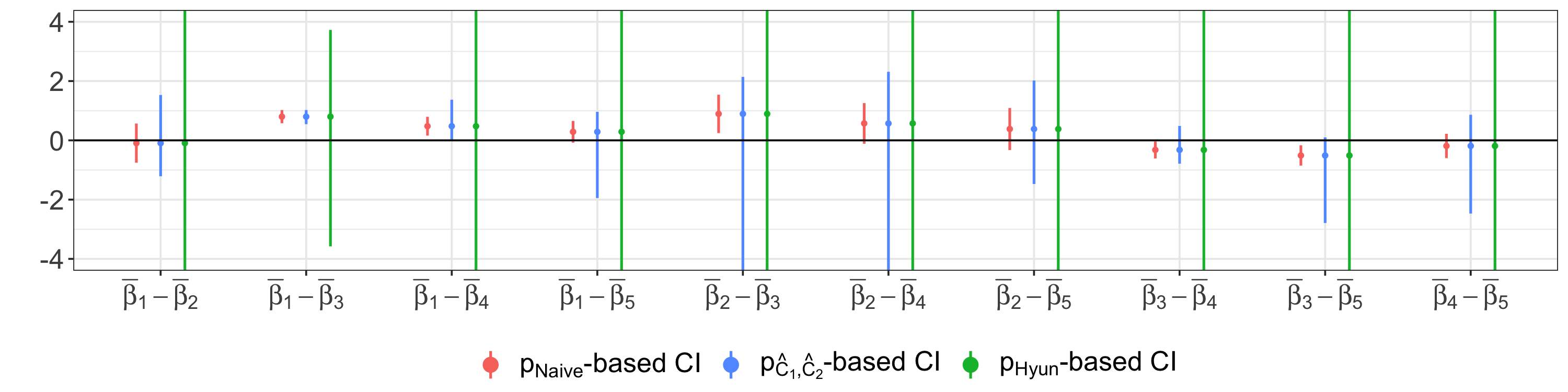
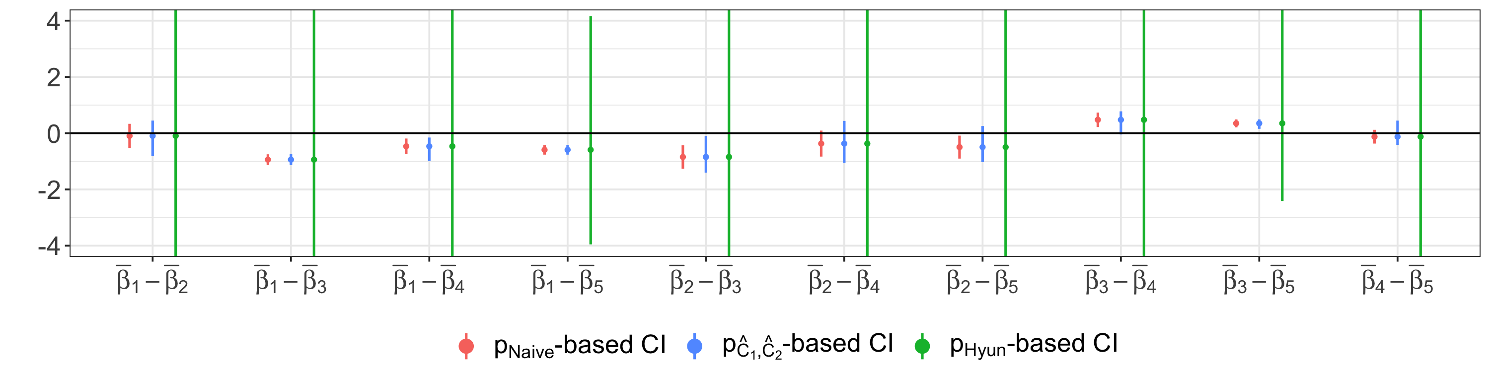
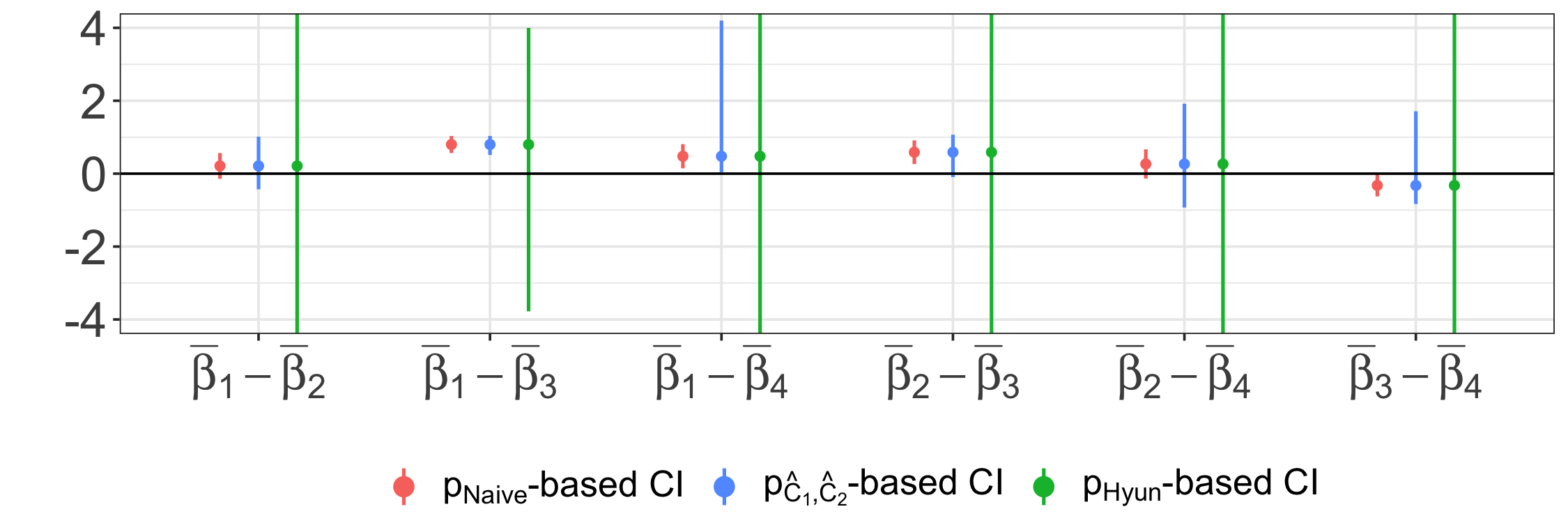
We assess the equality of the means of each pair of connected components using in (21), in (10), and in (11). The results are in Figure 5(c). The subset of pairs for which is below and is not is displayed in bold. For instance, the Northeast () and the Southeast () have a statistically significant difference in mean drug overdose death rates using the test based on , but not using the test based on , at level . Confidence intervals corresponding to these -values are displayed in Figure 5(d). Intervals based on are much wider than those based on across all ten pairs of connected components. In addition, the confidence intervals based on are not much wider than those based on , even though the latter do not have correct coverage for the true parameter .
(a) (b) (c)
 0.78
0.78
0.45
0.003
0.024
0.820
0.12
0.49
0.68
0.007
0.64
0.58
0.10
0.70
0.65
0.29
0.78
0.52
0.03
0.21
0.36
0.003
0.039
0.650
0.36
0.24
0.60
0.78
0.78
0.45
0.003
0.024
0.820
0.12
0.49
0.68
0.007
0.64
0.58
0.10
0.70
0.65
0.29
0.78
0.52
0.03
0.21
0.36
0.003
0.039
0.650
0.36
0.24
0.60
(d)
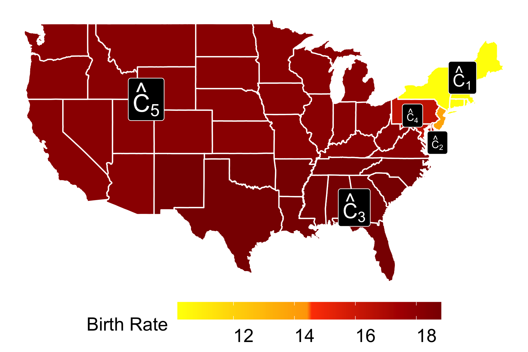
6.2 Teenage birth rates in the contiguous U.S. in 2018
Figure 6(a) displays the teenage birth rate in each of the 48 states. We solved the graph fused lasso with steps of the dual path algorithm, which results in five estimated connected components displayed in Figure 6(b); Appendix A.12 contains additional results for . For each pair of estimated connected components, we computed the -values , , and , along with the corresponding confidence intervals for the difference in means. The results are displayed in Figures 6(c) and (d).
As in Section 6.1, at level , the test based on makes more rejections than that based on . Additionally, the confidence intervals based on are much narrower than those based on ; in some cases, the former are of comparable length to those based on .
(a) (b) (c)
 0.67
0.99
0.74
0.005
0.26
0.13
0.24
0.26
0.02
0.10
0.24
0.04
0.71
0.002
0.61
0.34
0.38
0.71
0.67
0.99
0.74
0.005
0.26
0.13
0.24
0.26
0.02
0.10
0.24
0.04
0.71
0.002
0.61
0.34
0.38
0.71
(d)
7 Discussion
We have proposed a new procedure for testing for the difference in the means of two connected components resulting from the graph fused lasso. Our approach conditions on less information than existing approaches, leading to substantially higher power while still controlling the selective Type I error.
Methods developed in this paper are implemented in the R package GFLassoInference. Instructions on how to download and use this package can be found at https://yiqunchen.github.io/GFLassoInference. Code and files to reproduce the results in the paper can be found at https://github.com/yiqunchen/GFLassoInference-experiment.
7.1 Incorporating the selection of the tuning parameter
Throughout this paper, we have chosen , the number of steps in the dual path algorithm for (3), without making use of the data. However, in practice, the tuning parameter is often selected based on the data. For instance, we could choose the value of that minimizes the modified Bayesian information criterion [Hyun et al.,, 2018, Zhang and Siegmund,, 2007]. We can extend our idea in Section 3 to obtain a -value similar to (11) that also conditions on the value of adaptively-chosen (or , the number of connected components in ).
7.2 Extension to other generalized lasso problems
Ideas in this paper apply beyond the setting of the piecewise constant model in (1) and the graph fused lasso estimator in (3). For instance, we can consider extending our proposal to the trend filtering problem, which postulates that the underlying signal is ordered and piecewise polynomial [Tibshirani,, 2014, Kim et al.,, 2009]. Because trend filtering is a special case of (2) and can be solved using the dual path algorithm, an extension of the approach in Section 3 can be applied.
In addition, we can extend our proposal from an identity matrix in (2) to any design matrix with full column rank, i.e., . Hyun et al., [2018] showed that a -value similar to (10) can be used in this case to test the hypothesis (4). Therefore, we can directly apply the computational insights in Section 3 to obtain a more powerful test.
7.3 Relaxing assumptions in (1)
While the idea of conditioning on less information to improve the power of a selective inference procedure applies regardless of the distributions of the observations, the assumptions in model (1) are critical to the proof of Proposition 3, and therefore, the efficient computation of . A line of recent work in selective inference has focused on relaxing these assumptions in high-dimensional linear modeling [Tibshirani et al.,, 2018, Tian and Taylor,, 2018, Charkhi and Claeskens,, 2018], and may be applicable to the generalized lasso. Alternatively, we can extend (1) to other exponential family distributions by leveraging the recent developments in generalized data carving [Rasines and Alastair Young,, 2021, Leiner et al.,, 2021, Schultheiss et al.,, 2021].
8 Acknowledgments
We thank the authors of Le Duy and Takeuchi, [2021] for providing us with their software implementation. This work was partially supported by National Institutes of Health grants [R01EB026908, R01DA047869] and a Simons Investigator Award to D.W.
References
- Amin et al., [2017] Amin, R., Decesare, J. Z., Hans, J., and Roussos-Ross, K. (2017). Epidemiologic surveillance of teenage birth rates in the United States, 2006-2012. Obstetrics and Gynecology, 129(6):1068–1077.
- Arnold and Tibshirani, [2016] Arnold, T. B. and Tibshirani, R. J. (2016). Efficient implementations of the generalized lasso dual path algorithm. J. Comput. Graph. Stat., 25(1):1–27.
- [3] Centers for Disease Control and Prevention (2020a). 2018 Drug Overdose Death Rates. https://www.cdc.gov/drugoverdose/data/statedeaths/drug-overdose-death-2018.html.
- [4] Centers for Disease Control and Prevention (2020b). 2018 Teenage Birth Rates. https://www.cdc.gov/nchs/pressroom/sosmap/teen-births/teenbirths.htm.
- Charkhi and Claeskens, [2018] Charkhi, A. and Claeskens, G. (2018). Asymptotic post-selection inference for the Akaike information criterion. Biometrika, 105(3):645–664.
- Chen and Bien, [2020] Chen, S. and Bien, J. (2020). Valid inference corrected for outlier removal. J. Comput. Graph. Stat., 29(2):323–334.
- Fithian et al., [2014] Fithian, W., Sun, D., and Taylor, J. (2014). Optimal inference after model selection. arXiv preprint arXiv:1410.2597.
- Friedman et al., [2007] Friedman, J., Hastie, T., Höfling, H., and Tibshirani, R. (2007). Pathwise coordinate optimization. Ann. Appl. Stat., 1(2):302–332.
- Gao et al., [2020] Gao, L. L., Bien, J., and Witten, D. (2020). Selective inference for hierarchical clustering. arXiv preprint arXiv:2012.02936.
- Harchaoui and Lévy-Leduc, [2010] Harchaoui, Z. and Lévy-Leduc, C. (2010). Multiple change-point estimation with a total variation penalty. J. Am. Stat. Assoc., 105(492):1480–1493.
- Hastie et al., [2015] Hastie, T., Tibshirani, R., and Wainwright, M. (2015). Statistical learning with sparsity: the lasso and generalizations. Chapman and Hall/CRC.
- Hyun et al., [2018] Hyun, S., G’Sell, M., and Tibshirani, R. J. (2018). Exact post-selection inference for the generalized lasso path. Electron. J. Stat., 12(1):1053–1097.
- Hyun et al., [2021] Hyun, S., Lin, K. Z., G’Sell, M., and Tibshirani, R. J. (2021). Post-selection inference for changepoint detection algorithms with application to copy number variation data. Biometrics.
- Jewell et al., [2022] Jewell, S., Fearnhead, P., and Witten, D. (2022). Testing for a change in mean after changepoint detection. To appear in J. R. Stat. Soc. Series B Stat. Methodol.
- Johnson, [2013] Johnson, N. A. (2013). A dynamic programming algorithm for the fused lasso and -segmentation. J. Comput. Graph. Stat., 22(2):246–260.
- Kim et al., [2009] Kim, S.-J., Koh, K., Boyd, S., and Gorinevsky, D. (2009). trend filtering. SIAM Rev., 51(2):339–360.
- Le Duy and Takeuchi, [2021] Le Duy, V. N. and Takeuchi, I. (2021). More powerful conditional selective inference for generalized lasso by parametric programming. arXiv preprint arXiv:2105.04920.
- Lee et al., [2016] Lee, J. D., Sun, D. L., Sun, Y., and Taylor, J. E. (2016). Exact post-selection inference, with application to the lasso. The Annals of Statistics, 44(3):907–927.
- Leiner et al., [2021] Leiner, J., Duan, B., Wasserman, L., and Ramdas, A. (2021). Data blurring: sample splitting a single sample. arXiv preprint arXiv:2112.11079.
- Liu et al., [2018] Liu, K., Markovic, J., and Tibshirani, R. (2018). More powerful post-selection inference, with application to the lasso. arXiv preprint arXiv:1801.09037.
- Loftus and Taylor, [2014] Loftus, J. R. and Taylor, J. E. (2014). A significance test for forward stepwise model selection. arXiv preprint arXiv:1405.3920.
- Mehrizi and Chenouri, [2021] Mehrizi, R. V. and Chenouri, S. (2021). Valid post-detection inference for change points identified using trend filtering. arXiv preprint arXiv:2104.12022.
- Ramdas and Tibshirani, [2016] Ramdas, A. and Tibshirani, R. J. (2016). Fast and flexible ADMM algorithms for trend filtering. J. Comput. Graph. Stat., 25(3):839–858.
- Rasines and Alastair Young, [2021] Rasines, D. G. and Alastair Young, G. (2021). Splitting strategies for post-selection inference. arXiv preprint arXiv:2102.02159.
- Reid et al., [2017] Reid, S., Taylor, J., and Tibshirani, R. (2017). Post-selection point and interval estimation of signal sizes in Gaussian samples. Can. J. Stat., 45(2):128–148.
- Rinaldo, [2009] Rinaldo, A. (2009). Properties and refinements of the fused lasso. The Annals of Statistics, 37(5B):2922–2952.
- Rudin et al., [1992] Rudin, L. I., Osher, S., and Fatemi, E. (1992). Nonlinear total variation based noise removal algorithms. Physica D.: Nonlinear Phenomena, 60(1):259–268.
- Sadhanala et al., [2016] Sadhanala, V., Wang, Y.-X., and Tibshirani, R. J. (2016). Total variation classes beyond 1d: Minimax rates, and the limitations of linear smoothers. Advances in Neural Information Processing Systems 29, pages 3513–3521.
- Schieber et al., [2019] Schieber, L. Z., Guy, G. P., Seth, P., Young, R., Mattson, C. L., Mikosz, C. A., and Schieber, R. A. (2019). Trends and patterns of geographic variation in opioid prescribing practices by state, United States, 2006-2017. JAMA Network Open, 2(3):e190665–e190665.
- Schultheiss et al., [2021] Schultheiss, C., Renaux, C., and Bühlmann, P. (2021). Multicarving for high-dimensional post-selection inference. Electron. J. Stat., 15(1):1695 – 1742.
- Tian and Taylor, [2018] Tian, X. and Taylor, J. (2018). Selective inference with a randomized response. The Annals of Statistics, 46(2):679–710.
- Tibshirani, [1996] Tibshirani, R. (1996). Regression shrinkage and selection via the lasso. J. R. Stat. Soc. Series B Stat. Methodol., 58(1):267–288.
- Tibshirani et al., [2005] Tibshirani, R., Saunders, M., Rosset, S., Zhu, J., and Knight, K. (2005). Sparsity and smoothness via the fused lasso. J. R. Stat. Soc. Series B Stat. Methodol., 67(1):91–108.
- Tibshirani, [2014] Tibshirani, R. J. (2014). Adaptive piecewise polynomial estimation via trend filtering. The Annals of Statistics, 42(1):285–323.
- Tibshirani et al., [2018] Tibshirani, R. J., Rinaldo, A., Tibshirani, R., and Wasserman, L. (2018). Uniform asymptotic inference and the bootstrap after model selection. The Annals of Statistics, 46(3):1255–1287.
- Tibshirani and Taylor, [2011] Tibshirani, R. J. and Taylor, J. (2011). The solution path of the generalized lasso. The Annals of Statistics, 39(3):1335–1371.
- Tibshirani et al., [2016] Tibshirani, R. J., Taylor, J., Lockhart, R., and Tibshirani, R. (2016). Exact post-selection inference for sequential regression procedures. J. Am. Stat. Assoc., 111(514):600–620.
- Ventura et al., [2014] Ventura, S. J., Hamilton, B. E., and Matthews, T. J. (2014). National and state patterns of teen births in the United States, 1940-2013. National Vital Statistics Reports, 63(4):1–34.
- Xin et al., [2014] Xin, B., Kawahara, Y., Wang, Y., and Gao, W. (2014). Efficient generalized fused lasso and its application to the diagnosis of Alzheimer’s disease. In Twenty-Eighth AAAI Conference on Artificial Intelligence.
- Zhang and Siegmund, [2007] Zhang, N. R. and Siegmund, D. O. (2007). A modified Bayes information criterion with applications to the analysis of comparative genomic hybridization data. Biometrics, 63(1):22–32.
- Zhu, [2017] Zhu, Y. (2017). An augmented ADMM algorithm with application to the generalized lasso problem. J. Comput. Graph. Stat., 26(1):195–204.
Appendix A Appendix
A.1 Dual path algorithm for (2) with [Tibshirani and Taylor,, 2011]
-
1.
Compute .
-
2.
Compute .
-
3.
Update
-
4.
Record the solution :
-
5.
-
1.
Compute
-
2.
Compute hitting times .
-
3.
Set next hitting time , with the hitting coordinate .
-
4.
Compute
-
5.
Compute leaving times .
-
6.
Set next leaving time , leaving coordinate .
-
7.
Set .
-
8.
if then
Record the solution: :
A.2 Proof of Proposition 1
The proof of Proposition 1 is similar to the arguments in Section 6.2 of Tibshirani and Taylor, [2011].
We first prove the “if” direction:
| (24) |
First recall the result in (8), which states that . It follows that and , where denotes the th row of the matrix , written as a column vector. Therefore, to prove (24), it suffices to prove that
| (25) |
To prove (25), we first compute . The null space has dimension and admits the basis [Tibshirani and Taylor,, 2011], where the th element of equals Therefore, denoting the cardinality of the set , we have
It follows from algebra that
| (26) |
Now, according to the definition of and the assumption that and are in the same connected component, we have which implies that and therefore completes the proof for (25).
Next, we will prove the “only if” direction: that with probability one,
| (27) |
Combining the results in (8) and (26), we have that
| (28) |
We proceed to prove (27) by contradiction. Suppose without loss of generality that and we will show that, with probability one, . Combining our assumption and (28), we have that
| (29) |
By our assumption, is a non-zero vector. In addition, it follows from algebra that entries of the vector can only take values that are integer multiples of . Under model (1), , which implies that the inner product in (A.2) will be non-zero with probability one. Therefore, we have proven that with probability one, (27) holds.
A.3 Algorithm for computing in (14)
We now present an algorithm to compute (14).
-
1.
, , .
-
2.
, where was defined in (9).
-
3.
while do
-
(a)
Compute .
-
(b)
while do
-
i.
-
ii.
.
if then
.
while do
-
(a)
.
while do
-
i.
.
if then
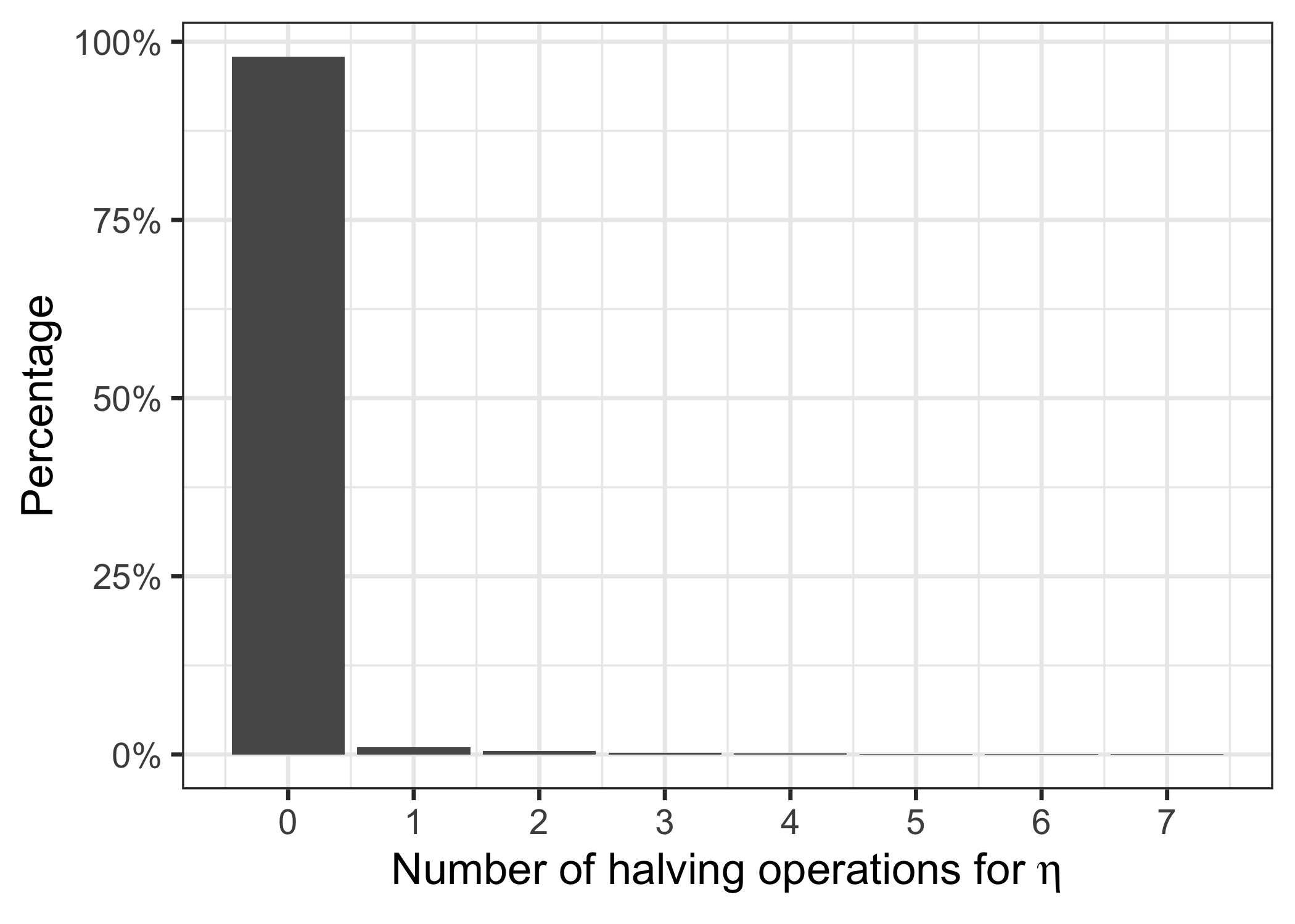
In Algorithm 2, we initialize with , and apply Corollary 1 to obtain the set (see step 4(a) in Algorithm 2 with ). If the left endpoint (where is a small constant set to by default), we repeat with a smaller value of (see step 4(b)i of Algorithm 2).
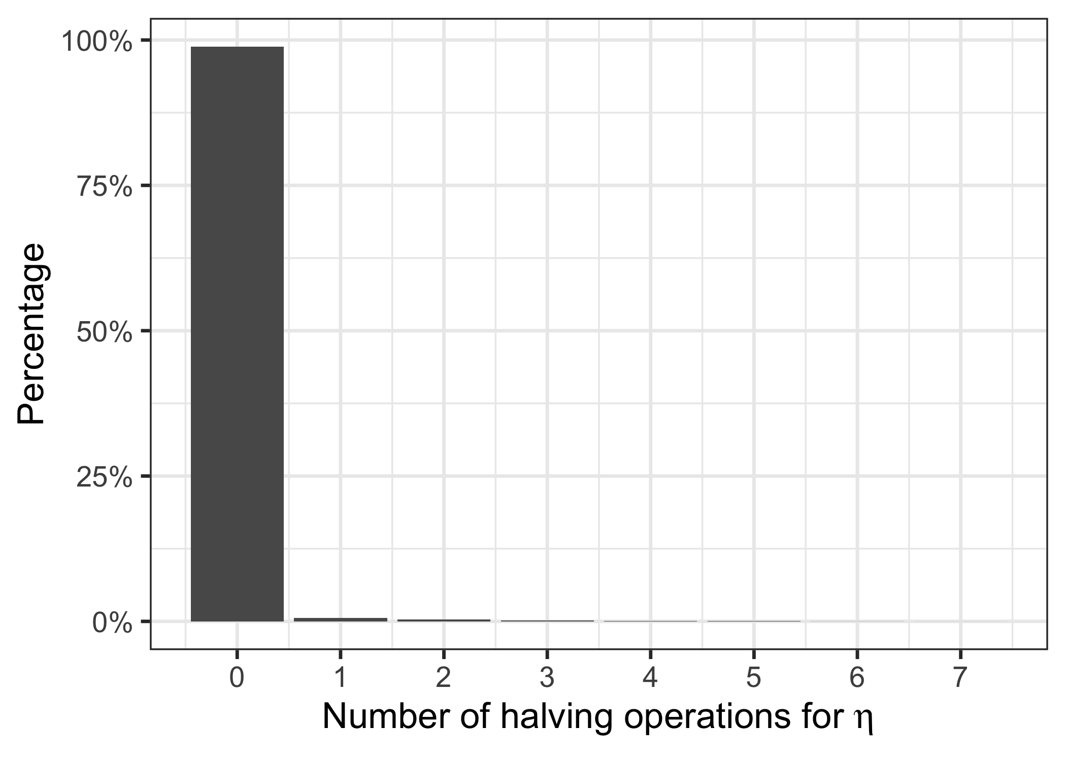
In a simulation study, we investigate how often, using the initialization , we need to perform the halving operation in step 4(b)i of Algorithm 2. Results are aggregated in Figure 7. We almost never have to halve the initial value , and the number of halving operations never exceeds seven.
A.4 Proof of Proposition 3
We first prove the statement (13). The following equalities hold for an arbitrary vector :
| (30) | ||||
Here, follows from the fact that , and the fact that we have conditioned on the event . To prove , we first note that and , which implies
where the notation is defined in (12). Finally, follows from the fact that implies independence of and .
Now under in (4), we have that
Here, step is the definition of in (11), and step follows from applying the result in (30). In , we used the fact that under , , which completes the proof.
Next, we will prove that the test that rejects when controls the selective Type I error as in (6). First of all, a test for the null hypothesis in (4) controls the selective Type I error in (6) if
| (31) |
In what follows, we will write as to emphasize that is a function of the observed difference in means . Using the result in (13), we have that
| (32) |
where is the cumulative distribution function of the magnitude of a random variable, truncated to the set .
Therefore, we have that, ,
| (33) | ||||
Step follows from (32) and step follows from (13) and letting denote the magnitude of a random variable, truncated to the set . Finally, in , we use the probability integral transform, which states that for a continuous random variable , is distributed as a Uniform(0,1) distribution.
Now for the test that rejects if , we have that
| (34) | ||||
In the proof above, step follows from the tower property of conditional expectation. To prove , we apply the results from (33).
A.5 Proof of Corollary 1 and Proposition 4
Proof.
Here, follows from Proposition 2, which states that the set for some matrix , where is interpreted as the component-wise inequality. Next, follows from the definition of in (12). Finally, and follow from solving the linear inequality in . Note that in , we implicitly assumed that (or ) such that (or ); if that doesn’t hold, the corresponding expression in is replaced by (or ).
∎
We proceed to prove Proposition 4.
where in , is the set of all possible outputs of the first steps of the dual path algorithm. In the proof above, is the definition of , and follows from the definition of . Furthermore, steps and follows from the definition of the index set (see (42)). Finally, to prove , we apply Corollary 1, which implies that for each , is an interval. This concludes the proof of Proposition 4.
A.6 Proof and an empirical analysis of Proposition 5
The proof of Proposition 5 is similar to the proof of Proposition 4 in \citetappendixjewell2019testing. First, note that by the definition of in Proposition 5, . Next, we have that
Here, follows from Bayes’ rule and the fact that , and is a direct consequence of the law of total probability. Step follows from the definition of , which implies that .
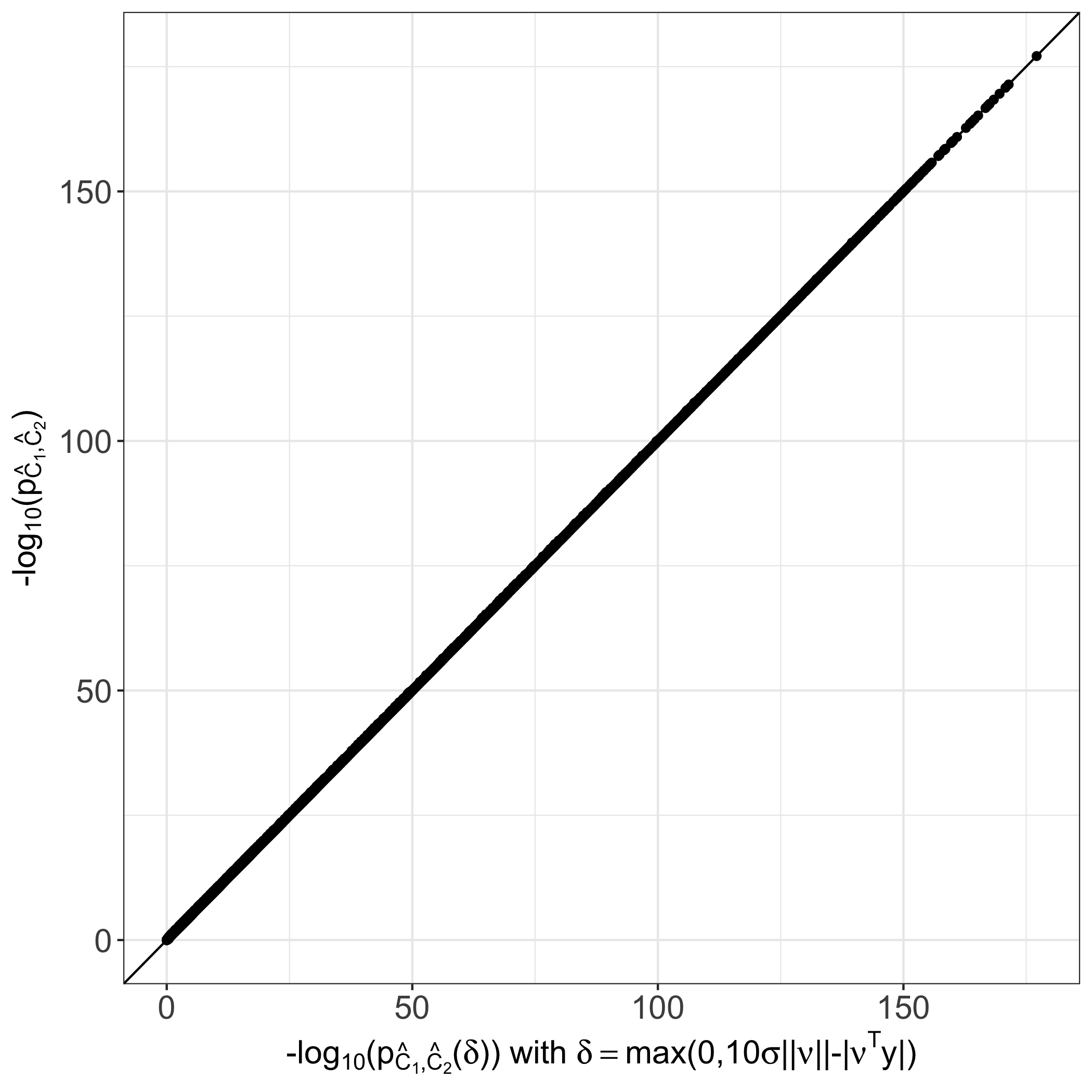
Next, we investigate the approximation error of using to compute the -value instead of . In what follows, we denote as for brevity. In prior work, several choices of has been proposed (e.g., [Jewell et al.,, 2022] and [Liu et al.,, 2018]). In this section, we computed with for the experiments in the one-dimensional fused lasso case (Section 5.1 of the main text). Results are aggregated and displayed in Figure 8. Panel (a) displays the -values versus with on the scale under the global null. We see that the two set of -values are nearly identical; the same holds for the datasets simulated with true changepoints (see Figure 8(b)). Regarding computational efficiency, this choice of reduces the overall running time of Algorithm 2 by 15–20%, depending on the specific simulation parameters. In conclusion, we suggest using to balance the inferential accuracy and computational efficiency.

A.7 Proof of Proposition 6
The proof of Proposition 6 is similar to the proof of Theorem 6.1 of \citetappendixLee2016-te and the proof of Corollary 3.1 of \citetappendixChen2020-rh.
Recalling the definition that is the cumulative distribution function of a random variable, truncated to the set defined in (14), we have that is a monotonically decreasing function of for each (see, e.g., Lemma A.2. of \citetappendixKivaranovic2020-ug). Since , it follows that and defined in (18) are unique, and that .
In addition, monotonicity implies that for all , (i) if and only if ; and (ii) if and only if . In other words, we have that
| (35) |
Now, under (1), , which implies that
In step , we use the fact that (35) holds for all ; therefore it holds for conditioning on the event as well. Next, step follows from (13) in the proof of Proposition 3, and letting denote a random variable, truncated to the set . The last step follows from the probability integral transform.
A.8 Modification of Algorithm 2 to compute
For the graph fused lasso with an arbitrary graph, it may be the case that for two integers , and \citepappendixTibshirani2011-fq. In other words, in (20) need not to be unique. Therefore, we cannot directly apply the recipes in Section 3 to characterize in (20).
In what follows, we propose to characterize a variant of that makes use of the smallest value of to yield exactly connected components:
| (36) |
We remark that the definitions of in (36) and in (20) coincide in the special case of the one-dimensional fused lasso, when the number of estimated connected components is uniquely determined by the number of steps in the dual path algorithm , and, as a result, is uniquely defined.
Using a similar argument to Proposition 3, we have that for ,
| (37) |
Therefore, the key to computing in (20) is to characterize the set
| (38) |
The algorithm for characterizing the set in (38) requires only minor modifications to Algorithm 2. Details are provided in Algorithm 3.
-
1.
, , .
-
2.
, where
-
3.
while do
-
(a)
Compute , where
-
(b)
while do
-
i.
-
ii.
, where
if then
while do
-
(a)
, where
while do
-
i.
, where
if then
Figure 9 displays the results for the test based on with for the two-dimensional fused lasso simulations described in Section 5.2. Panel (a) demonstrates that the test based on controls the selective Type I error. In panel (b) of Figure 9, we see that the test based on has substantially higher power than the test based on . Figures 9(c) and (d) investigate the detection probability (defined in (40)) and conditional power (defined in (39)) of .


A.9 Additional power comparisons
In Section 5, we considered the power of the tests based on and as a function of the binned effect size . Here, we conduct three additional analyses on the same simulated datasets from Section 5.
In the first analysis, we separately consider two quantities considered in prior work \citepappendixGao2020-yt,jewell2019testing,Hyun2018-gx: (i) the detection probability (i.e., the probability that and are true piecewise constant regions in the original signal ) of the graph fused lasso estimator in Eq. (3) of the main manuscript, and (ii) the conditional power of the tests based on and (i.e., the probability of rejecting , given that and are true piecewise constant regions).
Given simulated datasets, we can estimate the conditional power as
| (39) |
where and correspond to the -values and estimated connected components under consideration for the th simulated dataset. Here, is the th true piecewise constant segment in . Because the quantity in (39) conditions on the event that and correspond to true piecewise constant segments, we also estimate how often this occurs:
| (40) |
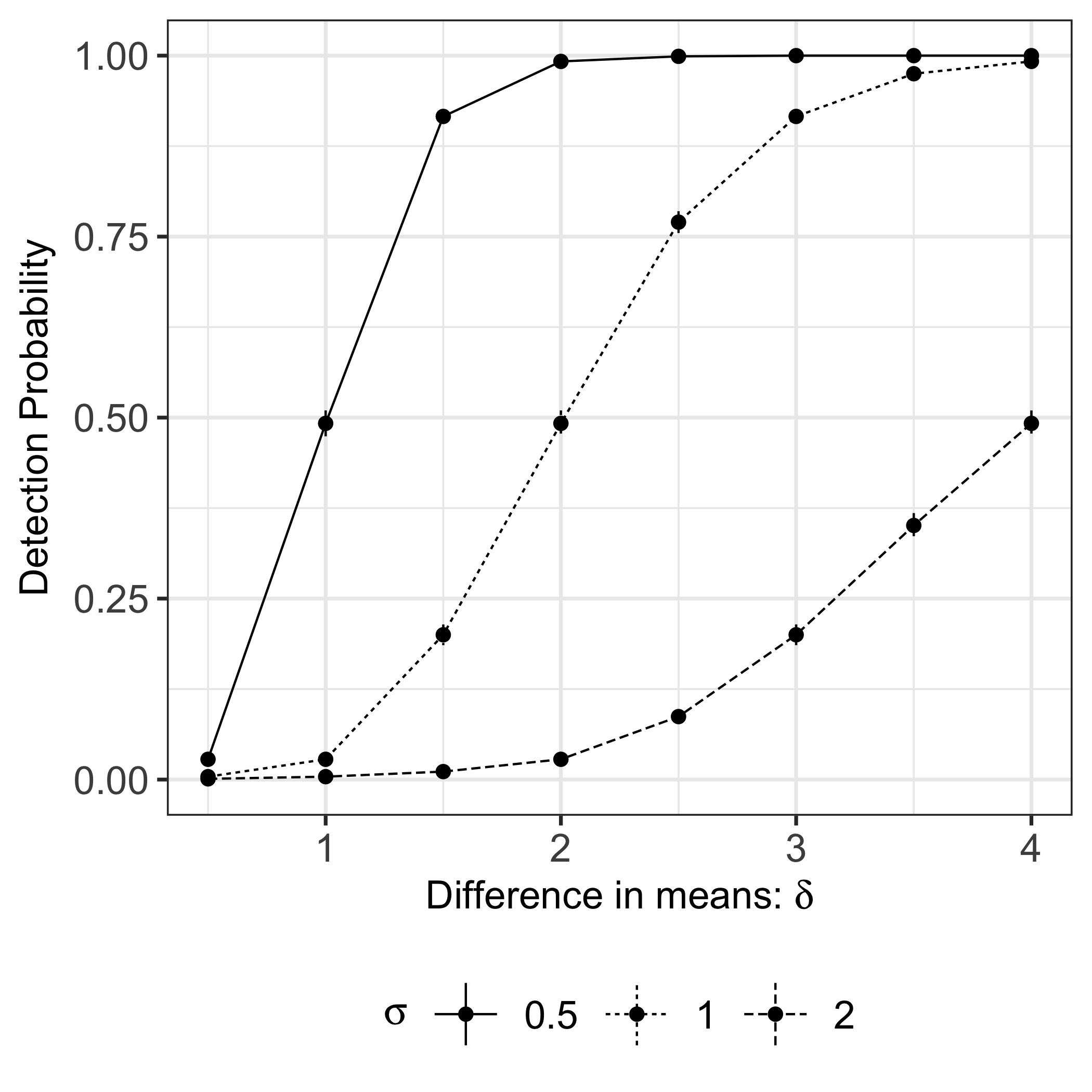
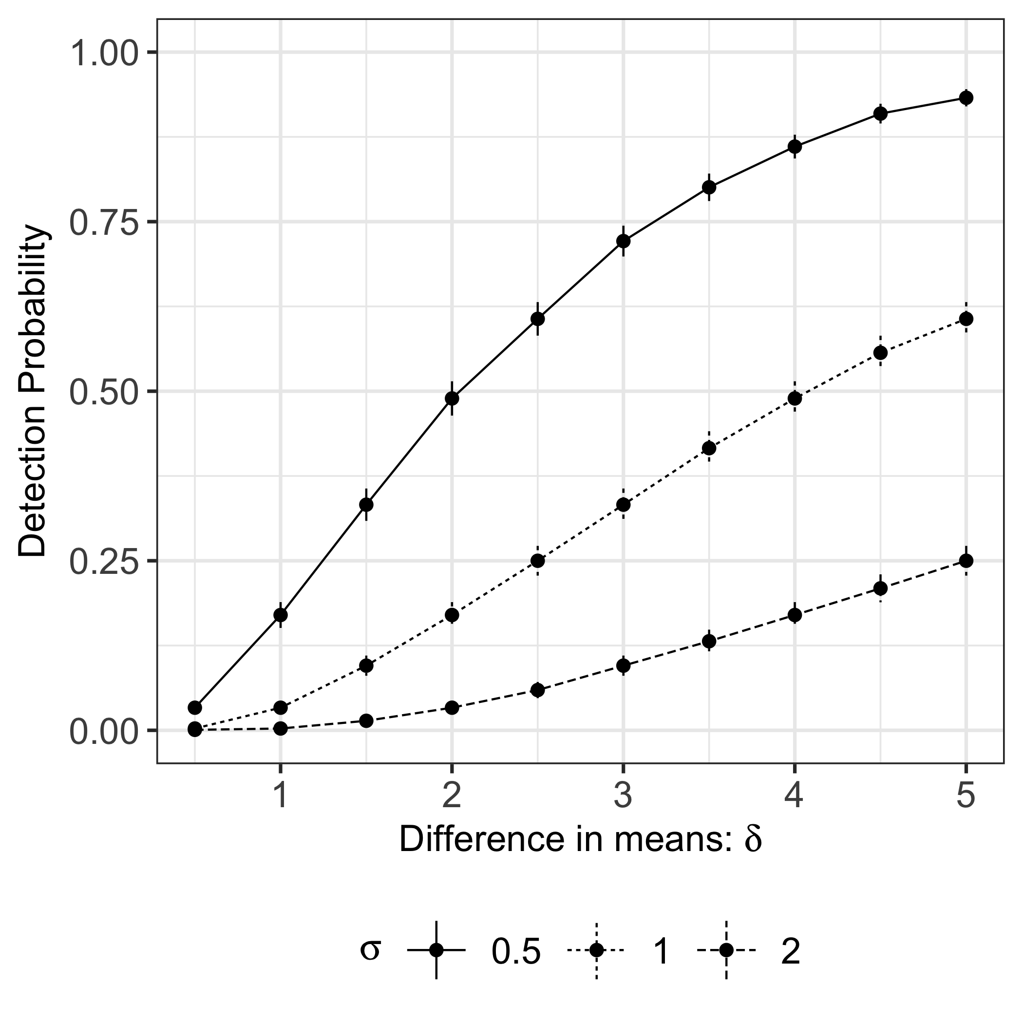
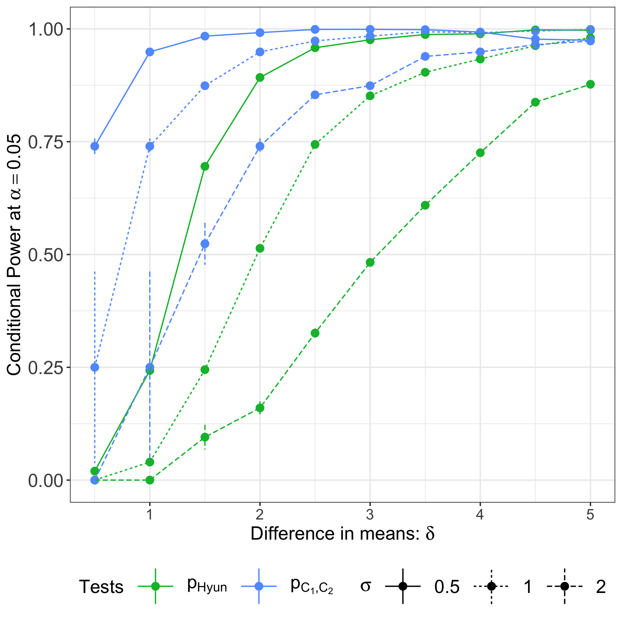
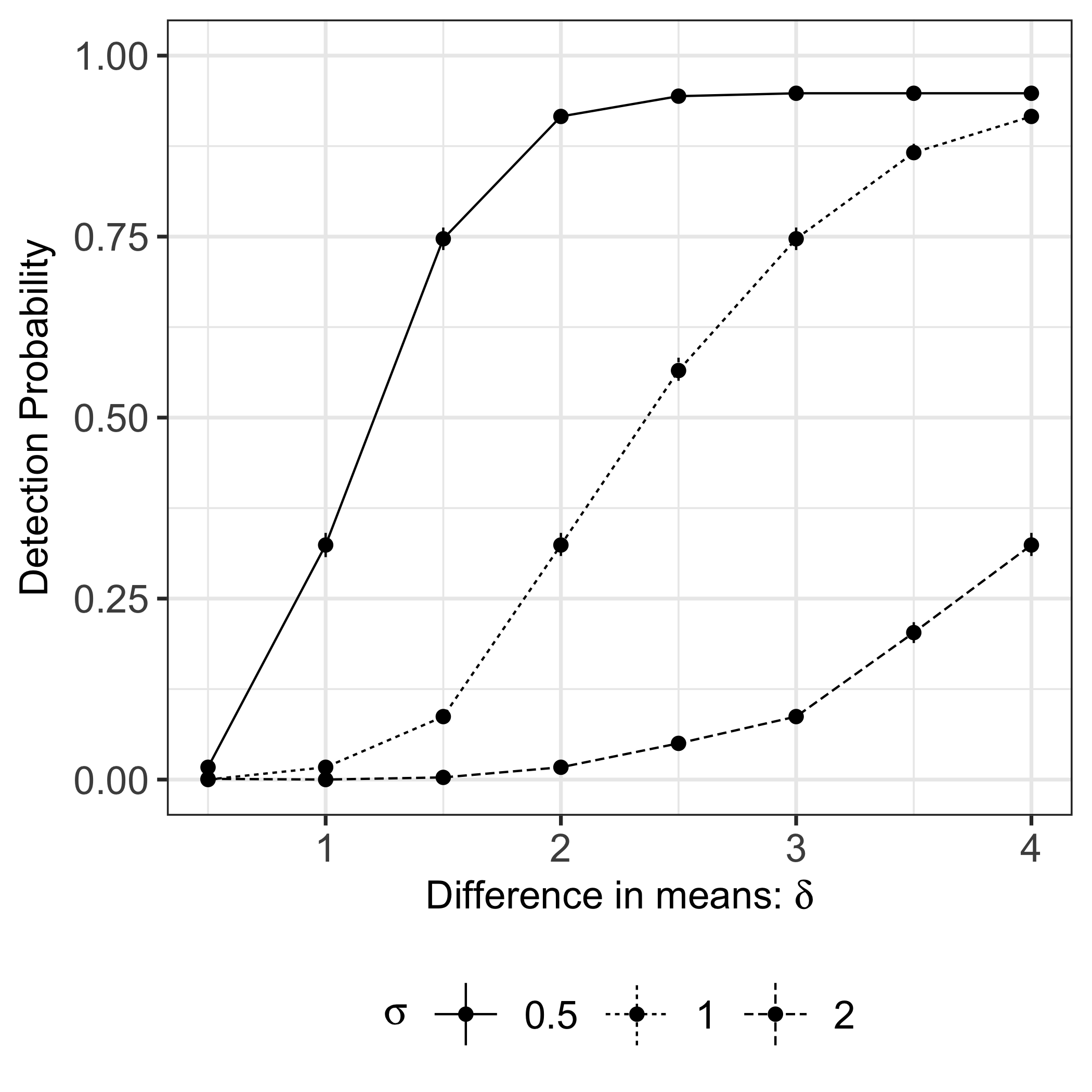
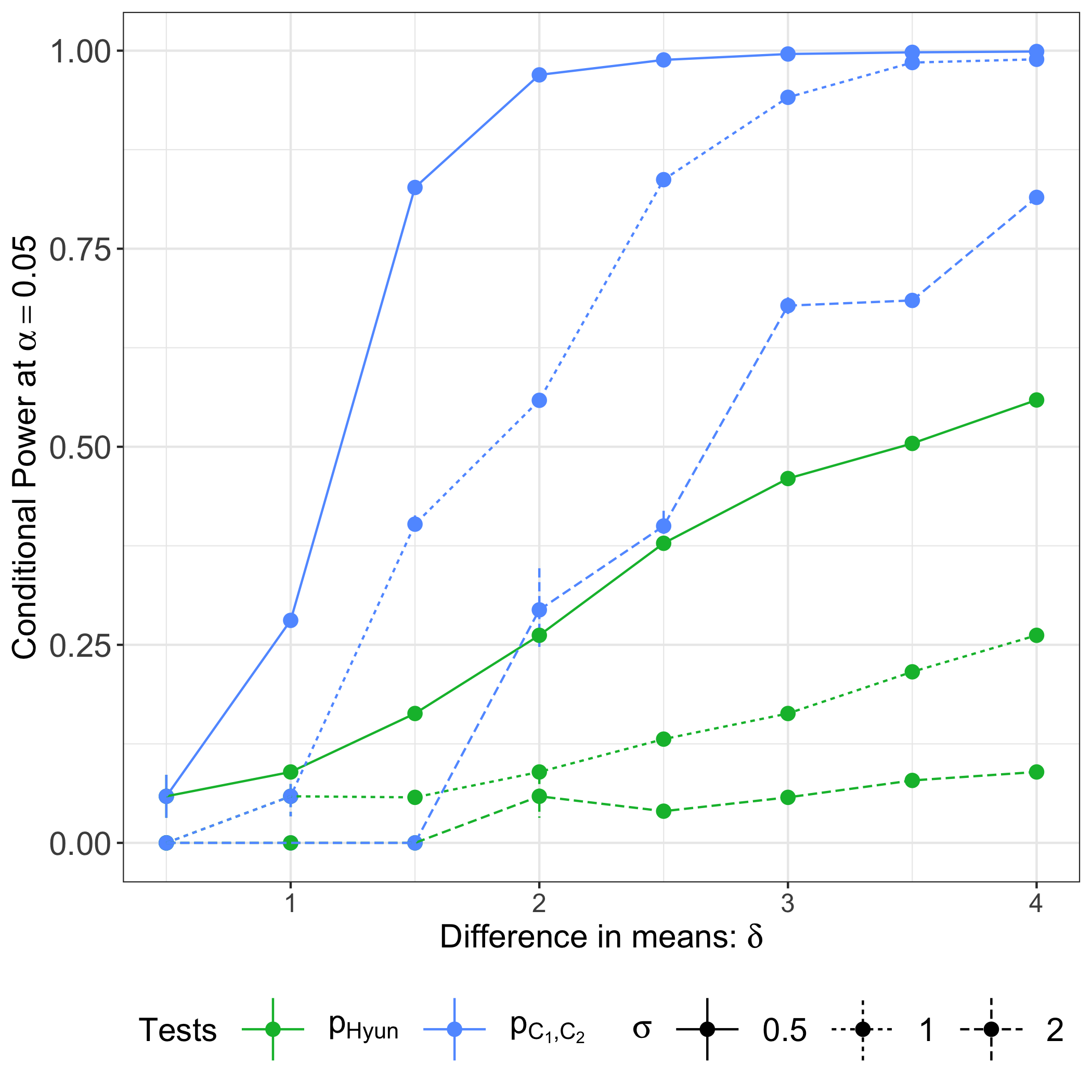
We evaluated detection probability and conditional power on data generated from the one-dimensional and two-dimensional fused lasso models, with the same simulation setup as in Sections 5.1 and 5.2, respectively. Results aggregated over 1,500 simulations are displayed in Figure 10. Panels (a) and (b) display the detection probability and conditional power (with ) for the one-dimensional fused lasso, respectively. Both quantities increase as the difference in means between the two piecewise constant segments ( in (22)) increases. By contrast, both quantities decrease as the variance increases. In addition, for a given value of and , the conditional power of the test based on is higher than that based on . We observe similar trends in the two-dimensional fused lasso case; see Figure 10(c)–(d).
In the second analysis, instead of binning , we fit a regression spline using the gam function in the R package mgcv \citepappendixwood_2017 to obtain a smooth estimate for the one-dimensional fused lasso simulations in Section 5.1.2. The results are in Figure 11. As in Figure 3(c), the power of the tests that reject if or is below increases as increases. For a given value of , the test based on has higher power than that based on .
Finally, in the third analysis, we assess the sensitivity of our conclusions to the choice of in the dual path algorithm, using the one-dimensional fused lasso model in (22). Recall that in Section 5.1, we choose so the number of estimated connected components resulting from the one-dimensional fused lasso equals the true number of connected components in (22).
Here, we repeat the experiments in Section 5.1 with , which yields five estimated connected components. Results are displayed in Figure 12. Panel (a) displays the observed -value quantiles versus Uniform(0,1) quantiles, aggregated over 1,000 simulated datasets. As in the case of , only tests based on or control the selective Type I error. In Figure 12(b), we see that the power of the tests based on or increases as increases. For a given value of , the test based on has substantially higher power than the test based on . In other words, the substantial increase in power, as well as the selective Type I error control, of the test based on , does not depend on correctly specifying .

A.10 Estimation of the error variance in (1)
Throughout this section, we have assumed that in (1) is known. In practice, we can plug in an estimate when computing the -values and . That is, we use
| (41) |
where .
In this section, we investigate the empirical selective Type I error control and power of the following estimators of :
-
•
, where are the estimated connected components of the graph fused lasso solution ;
-
•
, where is the mean of the data ; and
-
•
, where , and .
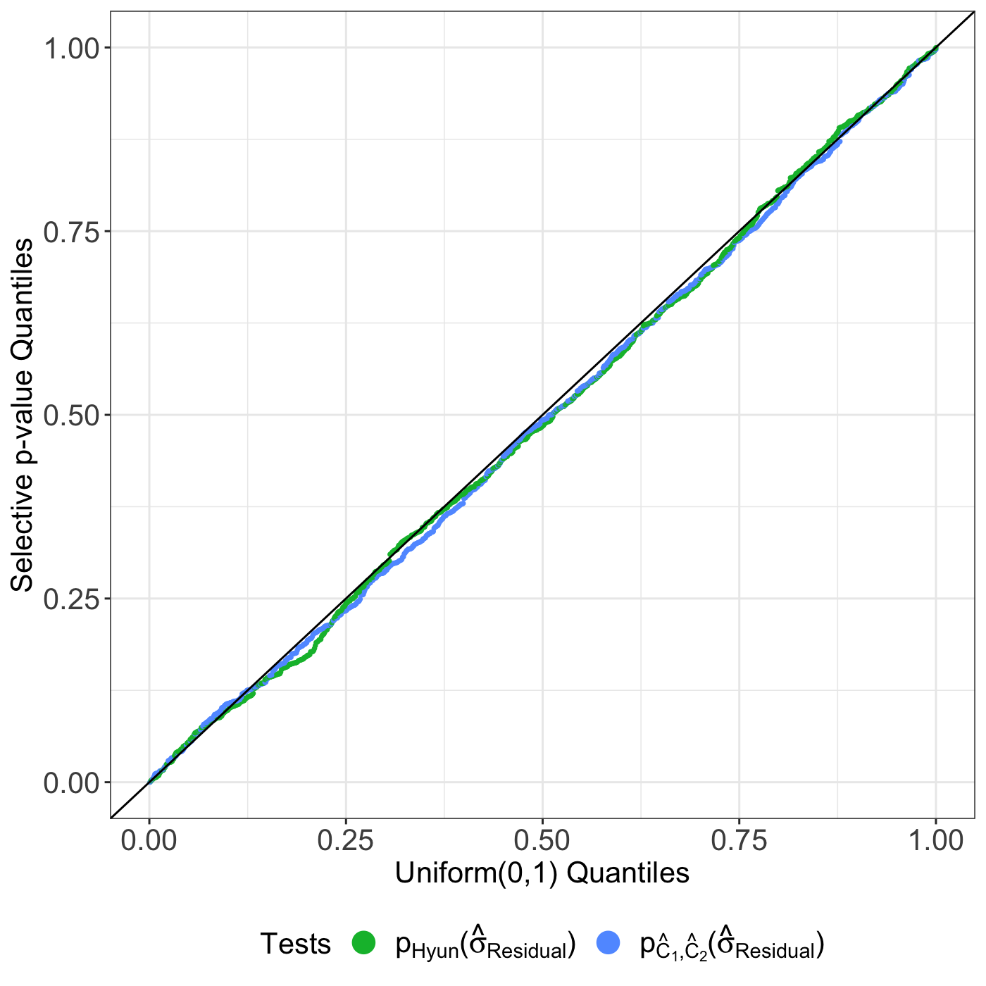

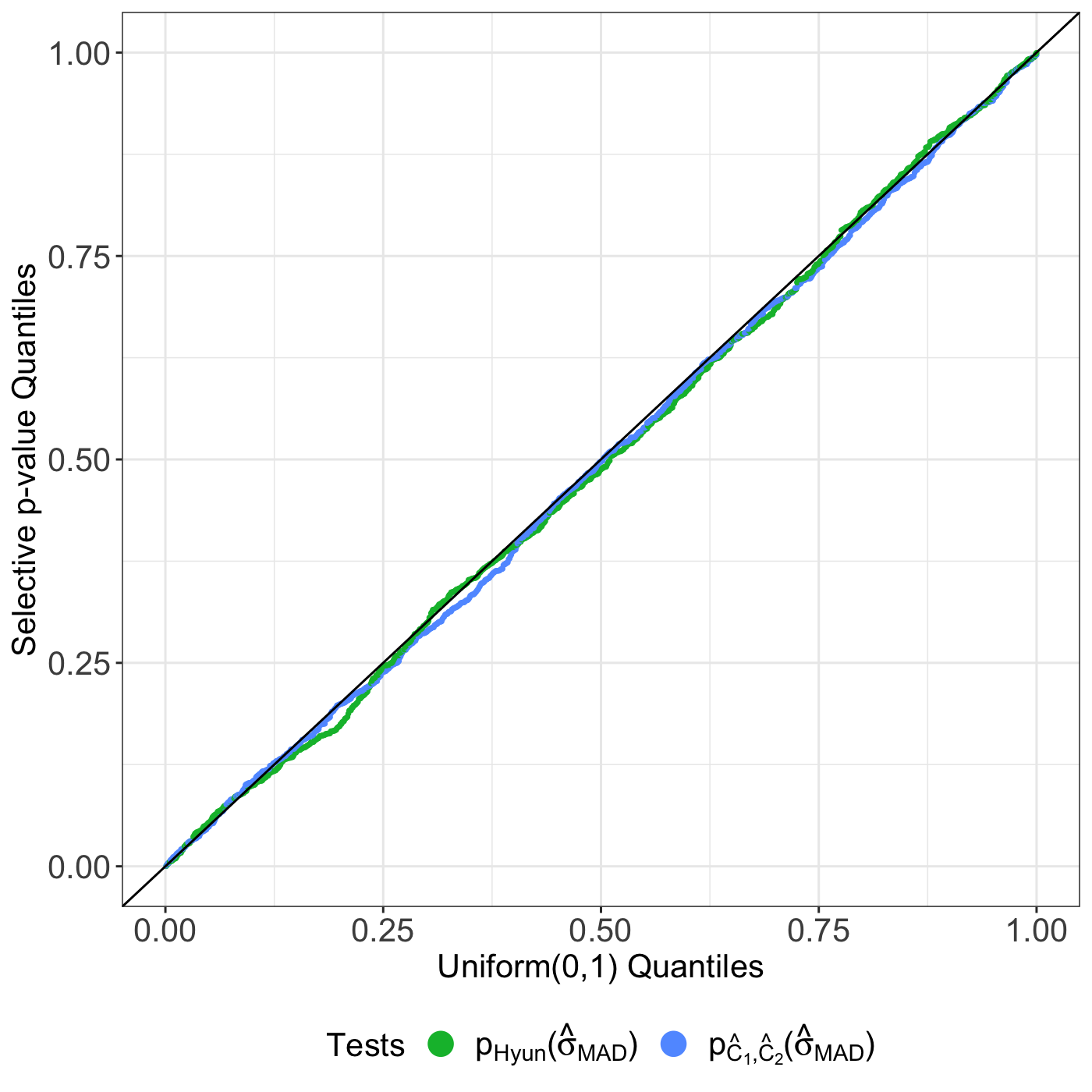
Figure 13 displays the quantiles of the -values and computed using the estimated variances with the same simulation setup as in Section 5.1.1. All three estimators ( with , , and ) lead to selective Type I error control under the global null.
In addition, we compared the power of the tests based on estimated variance with that obtained using the true variance. Results from a simulation study with the same setup as in Section 5.1.2 are aggregated in Figure 14. We see that the tests based on with or result in nearly identical power to the test based on the true variance . By contrast, using leads to a less powerful test, especially for larger values of . Moreover, the test based on is more powerful than the counterpart based on , regardless of the chosen variance estimator.
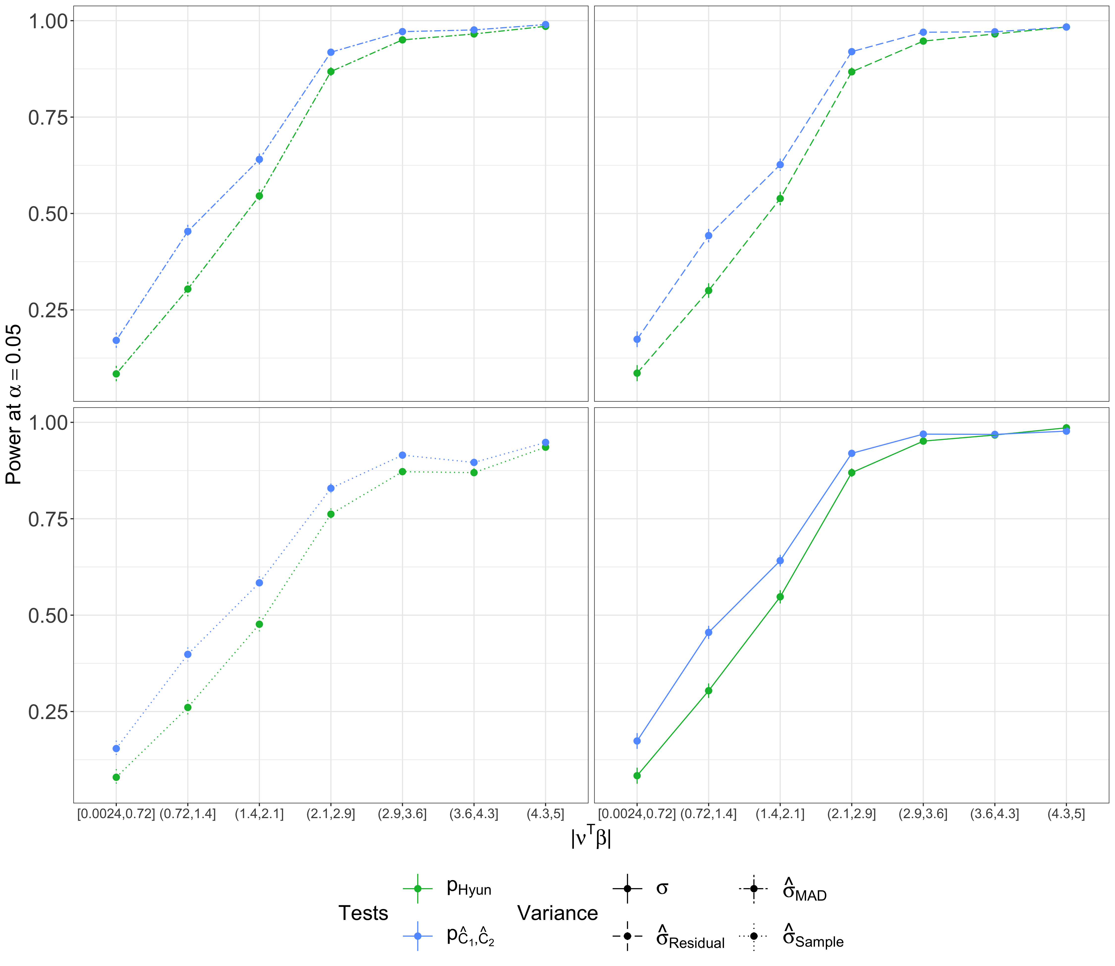
Our empirical results agree with observations made in related problems for selective inference: (i) when the global null does not hold, is a conservative estimator of the true variance \citepappendixTibshirani2018-rr,Hyun2018-gx,Gao2020-yt,Rugamer2020-fz; (ii) has good empirical performance when is correctly specified; and (iii) in the case of the one-dimensional fused lasso, is an asymptotically consistent estimator under appropriate assumptions \citepappendixKovacs2020-qb,jewell2019testing.
A.11 Timing complexity for Algorithm 2
In this section, we first characterize the computational complexity of Algorithm 2 using the following Proposition.
Proposition 7.
We omit the proof of Proposition 7, as it directs follows from Algorithm 2 and the definition of . Proposition 7 implies that the time complexity for Algorithm 2 is instance-dependent, and can in principle be prohibitively large. For instance, in the one-dimensional fused lasso case, is upper bounded by , where is the number of observations, and is the number of steps in the dual path algorithm. However, in practice, we are nowhere near this worst case scenario: in the experiments in Section 5, is of reasonable size. In particular, for the one-dimensional fused lasso simulations described in Section 5.1.1, the upper bound postulates that can be as large as (). However, as displayed in Figure 15(a), empirically, falls under 500 in all instances.
In addition, because we re-implemented the polyhedron approach in \citetappendixHyun2018-ta using the ideas from \citetappendixArnold2016-ue, each graph fused lasso instance and its corresponding intervals of the form (see Section 3 for more details) can be computed efficiently.
Figure 15(b) displays the running time of Algorithm 2, computed on a MacBook Pro with a 1.4 GHz Intel Core i5 processor, over 1,000 replicate datasets simulated according to the one-dimensional fused lasso model in Section 5.1.1 with . The graph fused lasso problem is solved using the the dual path algorithm with . The average running time for running Algorithm 2 to test each hypothesis is 2.7 seconds.
When the empirical size of defined in (42) is large, we could alternatively use an importance sampling approach to obtain an approximate -value with ideas from, e.g., \citetappendixYang2016-km,Rugamer2022-yz,Rugamer2020-fz.

A.12 Additional results for data applications
Here, we repeat the analysis in Sections 6.1 and 6.2 with and , respectively. Results are displayed in Figures 16 and 17. Similar to the case of , the test based on leads to more rejections than the test based on at . Furthermore, the confidence intervals based on are considerably shorter than those based on , and in some cases, even comparable to the naive confidence intervals that do not have proper coverage for the true parameter .
(a) (b) (c)
 0.24
0.22
0.59
0.005
0.02
0.82
0.04
0.73
0.20
0.27
0.69
0.04
0.50
0.36
(d)
0.24
0.22
0.59
0.005
0.02
0.82
0.04
0.73
0.20
0.27
0.69
0.04
0.50
0.36
(d)
(a) (b) (c)
 0.67
0.99
0.74
0.07
0.26
0.13
0.34
0.26
0.02
0.65
0.24
0.12
0.71
0.14
0.61
0.34
0.78
0.71
(d)
0.67
0.99
0.74
0.07
0.26
0.13
0.34
0.26
0.02
0.65
0.24
0.12
0.71
0.14
0.61
0.34
0.78
0.71
(d)
A.13 A comparison of and
In this section, we first briefly review the -value proposal of \citetappendixLe_Duy2021-iy (henceforth referred to as ), and elaborate on the conceptual differences between and (11). Next, we provide results from a simulation study that compares the selective Type I error (6) and the power of the tests based on , , and . In the simulations that follow, we will only consider the one-dimensional fused lasso problem, since the extension to a non-chain graph has not been implemented by \citetappendixLe_Duy2021-iy at the time of writing. We used the software for computing provided by the authors at https://github.com/vonguyenleduy/parametric_generalized_lasso_selective_inference.
A.13.1 A conceptual comparison of and
Le_Duy2021-iy consider the -value defined as
| (43) |
where, with a slight abuse of notation, is the solution to (2) with data . Using a similar argument to Proposition 3, they showed that (43) can be recast as the cumulative distribution function of a random variable, truncated to a set that can be efficiently computed. We note that in the case of the graph fused lasso (3), the set is equivalent to the set of edges used to determine the connected components of ; in other words, conditioning on the event is equivalent to conditioning on , for an appropriate choice of \citepappendixTibshirani2011-fq.
What advantages, then, does our proposal in (11) offer when compared to ?
-
•
Smaller conditioning set: first of all, we condition on even less information when constructing : conditions on the set of edges that are used to determine the connected components of , and therefore implicitly, on all of the connected components in (see, e.g., Proposition 1). By contrast, in (11), we condition only on the pair of connected components under investigation, thereby obtaining higher power.
-
•
Interpretability: the conditioning set for is based on the connected components of after running the dual path algorithm for steps. By contrast, conditions on the output of (3) with a specific . We argue that, as a result, is more interpretable. Consider the widely-popular one-dimensional fused lasso problem and a pair of estimated piecewise constant segments . answers the question:
Assuming that there is no difference between the population means of and , then what’s the probability of observing such a large difference in the sample means of and , given that and are among the piecewise constant segments estimated from the data?
On the other hand, answers the question:
Assuming that there is no difference between the population means of and , then what’s the probability of observing such a large difference in the sample means of and , given that and are among the piecewise constant segments estimated from the data with a specific ?
Here, is answering the question about piecewise constant segments, where is a very interpretable quantity (i.e., the number of estimated changepoints). In contrast, for , the meaning of could vary greatly across different datasets — the value of that yields estimated changepoints on one dataset could yield far more or fewer estimated changepoints on another dataset.
-
•
Numerical stability: \citetappendixLe_Duy2021-iy solved the primal problem (3) using an iterative solver, which in practice leads to numerical issues when identifying the set \citepappendixArnold2016-ue, and consequently, in computing . By contrast, we chose to work with the dual problem (7), which avoids these numerical issues and yields the exact connected components of when computing .
A.13.2 A simulation study comparing , , and
Next, we conducted a simulation study to compare the selective Type I error and power of the tests based on the following -values: in (10), in (11), and in (43). We tested the null hypothesis , where is defined in (5) for a randomly-chosen pair of adjacent piecewise constant segments , in the solution to the one-dimensional fused lasso problem.
The signal is piecewise constant with 10 changepoints (or equivalently, 11 piecewise constant segments), and the values of alternate between 0 and after each changepoint:
| (44) |
where and . Figure 18(a) displays an instance of (44) with and .
In the simulations that follow, the software accompanying \citetappendixLe_Duy2021-iy returned an empty string for for around 27% of the hypotheses. Upon inquiring, the authors of \citetappendixLe_Duy2021-iy said that this is due to numerical stability issues in identifying the conditioning set in . Consequently, the displayed results for are based on the subset of the hypotheses for which the authors’ software successfully returned a -value.
We first investigate the selective Type I error control by simulating from (44) with and . Therefore, the null hypothesis holds for all contrast vectors , regardless of the pair of piecewise constant segments under investigation. For and , we solved (3) with steps in the dual path algorithm, which yields exactly 11 piecewise constant segments by the properties of the one-dimensional fused lasso. For , we selected the tuning parameter so that (3) yields exactly 11 piecewise constant segments on the data.
Figure 18(b) displays the observed -value quantiles versus Uniform quantiles, aggregated over 1,000 hypothesis tests. We see that all three tests based on (10), (11), and (43) control the selective Type I error as in (6).
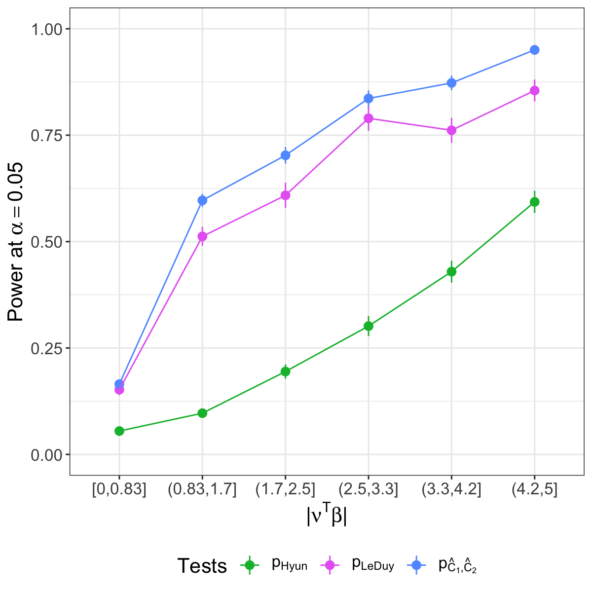
Next, we show that the test based on has higher power than the test based on , and both tests have higher power than the test based on . We generated 500 datasets from (44) for each of ten evenly-spaced values of . For each simulated dataset, we solved (3) with for , and , and chose the tuning parameter so that (3) yields 10 estimated changepoints for . We rejected the null hypothesis if the -value was less than . As in Section 5.1.2, we consider the power as a function of .
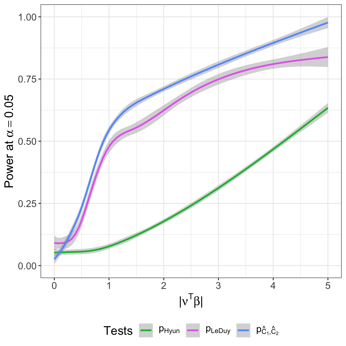
Figure 18(c) displays the power estimated by first creating six evenly-spaced bins of the observed values of , and then computing the proportion of simulated datasets for which we rejected within each bin. Alternatively, we could estimate the power as a smooth function of using a regression spline (see Figure 18(d)). In both cases, the test based on has 10–15% higher power than the test based , and both have substantially higher power than the test based on .
apalike \bibliographyappendixref.bib