The supremum principle selects simple, transferable models

Abstract

We consider how mathematical models enable predictions for conditions that are qualitatively different from the training data. We propose techniques based on information topology to find models that can apply their learning in regimes for which there is no data. The first step is to use the Manifold Boundary Approximation Method to construct simple, reduced models of target phenomena in a data-driven way. We consider the set of all such reduced models and use the topological relationships among them to reason about model selection for new, unobserved phenomena. Given minimal models for several target behaviors, we introduce the supremum principle as a criterion for selecting a new, transferable model. The supremal model, i.e., the least upper bound, is the simplest model that reduces to each of the target behaviors. We illustrate how to discover supremal models with several examples; in each case, the supremal model unifies causal mechanisms to transfer successfully to new target domains. We use these examples to motivate a general algorithm that has formal connections to theories of analogical reasoning in cognitive psychology.

One of the first important tasks in modeling data is selecting the form for a mathematical model. The form of the model defines the types of predictions a model can make and therefore–accurately or not–creates a type of “hypothesis space” called inductive bias Baxter (2000). In this study, we use the geometric and topological relationships among candidate models to reason about inductive bias and model selection. Of particular interest are predictions for qualitatively different conditions than those on which a model was trained, such as predicting a time series outside of the range of sampled time points, predicting under different experimental conditions, or applying insights from two populations to a third. A model’s ability to make such out-of-domain predictions is sometimes known as transferability, which is stronger than generalization, i.e., predicting data generated for inputs similar to those on which it was trained Weiss et al. (2016). We propose a general principle of model selection, the supremum principle, that encodes a preference for simplicity with respect to target quantities of interest while enabling model transferability and whose construction uses topological relationships formally equivalent to models of human analogical reasoning.

One of the key struggles of model selection is balancing inductive bias against model flexibility. Consider, for example, explaining the change in a cell’s state (e.g., healthy to cancerous) in terms of the proteome. A potential hypothesis space could include all possible interactions between all $\sim$25,000 known proteins. This has very little bias since the correct explanation is somewhere in this space; however, it would require an unreasonable amount of data to learn all the parameters of such a complex model. Furthermore, it would be even more difficult to interpret the model afterwards as most of the interactions are merely explanatory noise relative to the phenomenon of interest Batterman . Therefore, we seek to restrict the hypothesis space to the one that minimally includes our behavioral regimes of interest. Such a model doesn’t fit both states with one set of parameters, rather, it fits either set of data independently, i.e. some parameters could be unidentifiable to data from either state. In addition to describing cells in either state, this model predicts a mechanism for switching between them.

A minimal criterion for a useful predictive model is that it reproduces the training data within statistical noise, that is, a kind of coarse interpolation. Common statistical practices such as holdout, jackknife, and cross-validation reinforce this intuition. Sloppy models Brown and Sethna (2003); Brown et al. (2004); Waterfall et al. (2006); Machta et al. (2013), a class of over-parameterized models, further formalize the relation between prediction and interpolation using information geometry Amari and Nagaoka (2007); Transtrum et al. (2010). The predictions of sloppy models are controlled by only a few stiff parameter combinations and so are said to have a low effective dimensionalityTranstrum et al. (2010); LaMont and Wiggins (2019). Effective dimensionality is quantified in terms of widths of a model manifold, rigorous bounds for which are given by theorems from interpolation theory Transtrum et al. (2010); Quinn et al. (2019). Indeed, it has been suggested that predictive models are generalized interpolation schemes Transtrum et al. (2011a).

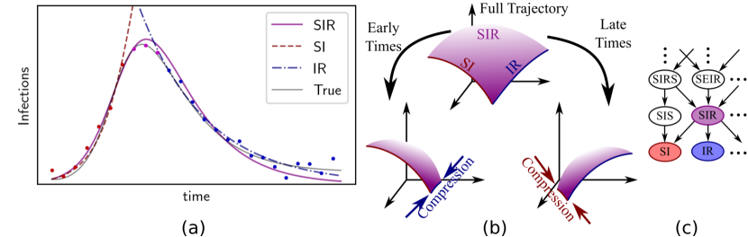
Figure 1: (a) Infections versus time for a hypothetical epidemic. Data taken at different times—early (red), late (blue), and intermediate (purple)—exhibit qualitatively different types of behaviors. These data carry information about different aspects of the generating process. The “True” curve represents the model from which data was generated, without the corruption of Gaussian noise. (b) Information geometry quantifies how data identify a model’s parameters. The full trajectory completely identifies an SIR model, manifest by a model manifold that is not compressed along either direction. Restricting to data at early times compresses the directions related to a recovery rate so that the model is well-approximated by an effective SI model. Similarly, restricting to late times compresses information about infection, leading to an effective IR model. (c) Candidate models of varying complexity can be arranged hierarchically in a directed graph. The SIR model is the supremum of the SI and IR models, i.e., the simplest model that combines information from both early and late times. It can use the information from data in two of the regimes to accurately predict a third.

However, there is a sense that more than simple interpolation ought to be possible Lake et al. (2017); Webb et al. (2020). Human cognition is driven by understanding, rather than mere pattern mimicry. When we reason about molecular bonds as if they were balls and springs, we use analogical reasoning to identify abstract relationships and transfer insights among superficially different systems. Can machines similarly analogize to make predictions of a qualitatively different nature than those on which they were trained?

To explore this question, we use information geometry to assess parameter identifiability and predictive performance for models fit to data from different regimes and reason about the hypotheses they encode. The Fisher Information Matrix (FIM) is information geometry’s fundamental object, a Riemannian metric on a manifold of models using parameters as coordinates Transtrum et al. (2010); Brouwer and Eisenberg (2018). Model manifolds are often thin, and boundaries correspond to simplified models, i.e., having fewer parameters Transtrum and Qiu (2014). Distances measured by the FIM typically compress the model manifold into a few relevant directions Machta et al. (2013) so that the manifold is thin and well-approximated by a low-dimensional, simplified model that resides on the boundary. Given training data, the Manifold Boundary Approximation Method (MBAM) explicitly finds limiting approximations to give a minimal, reduced model that encodes the information in the data. MBAM is an enabling technology for our approach and is described in detail elsewhere referencesTranstrum and Qiu (2014); Transtrum et al. (2015).

Given several reduced models for target quantities of interest, we next seek a single model that unifies their simplified explanations. To choose an appropriate model, we introduce the supremum principle: select the simplest model that is reducible to each of the target behaviors. One of the primary contributions of this paper is to show that this intuitive idea can be given a rigorous definition using the formalism of information topology. We call this model the supremal model and give an algorithm below for constructing it. The supremum principle formally encapsulates a preference for simplicity akin to Occam’s razor, motivated by the assumption that abstract models that explain multiple behaviors are more likely to transfer accurately to novel behaviors than models developed for a single phenomenon.

As a motivating example, consider modeling infection trajectories during an epidemic. Fig. 1a shows data generated from an MSEIR model with birth and death rates (six parameters, fifth-order dynamics) and corrupted by Gaussian noise. We partition the data into three qualitatively distinct regimes—early (red), intermediate (purple), and late (blue)—and ask: Which subsets of the data are informative for predicting data in another regime?

To illustrate the key principles, consider fitting the data with a simple SIR model (two parameters, second-order dynamics),

$$\frac{dS}{dt} =-\beta I\frac{S}{N}, \frac{dI}{dt} =-\gamma I+\beta I\frac{S}{N}, \frac{dR}{dt} =\gamma I.$$ (1)

When fitting to qualitatively different data, the two dimensional SIR model manifold is compressed depending on the informativity of the available data. The compression determines which parameters are identifiable from data and leads to an appropriate reduced model.

We focus on two reduced models on the boundary of the SIR model, shown in Fig. 1b. The first boundary segment, corresponding to $\gamma\rightarrow 0$, is the model with no recovery compartment, i.e., an “SI” model. Similarly, the “IR” model with $\beta\rightarrow\infty$ has a very fast infection rate. Consider only data from early times (red in Fig. 1). The FIM compresses the model manifold along the SI boundary segment, rendering the recovery rate $\gamma$ irrelevant. The approximate SI model (red dashed line in Fig. 1) has an effective infection rate that fits the early exponential growth . However, recovery data at later stages (blue), render $\beta$ irrelevant and are well approximated by the IR model.

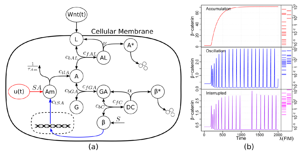
Figure 2: (a) A network diagram showing the “full” model of the Wnt pathway. The red indicates mechanisms that are unique to the accumulation model, and blue indicates mechanisms unique to the oscillation model. (b) Three possible behaviors of beta-catenin in response to Wnt. The accumulation Goentoro and Kirschner (2009) and oscillation Jensen et al. (2010) behaviors are known to occur naturally, while behaviors similar to the interrupted behavior have been reported in Riedel-Kruse et al. (2007); Gibb et al. (2009); Goldbeter and Pourquié (2008); Gomez et al. (2008); Rui et al. (2007).

The SI and IR models interpolate in their respective domains, but fail to transfer beyond those domains. The SIR model is the simplest that can interpolate all three regimes. Formally, the hierarchy of potential models forms a graded Partially Ordered Set (POSet). A POSet generalizes the concept of order within a set. Real numbers are completely ordered, that is $\forall a,b\in\mathbb{R}$, with $a\neq b$, either $a>b$ or $a<b$. POSets additionally allow for elements to be incomparable, i.e., neither $a>b$ nor $a<b$. Discrete POSets can be represented by a directed graph known as a Hasse diagram Transtrum et al. (2014) as in Fig. 1c. In this formalism, the SI and IR models are incomparable; there is no path in the directed graph connecting them. The SIR model is the supremum (i.e., least upper bound) of the SI and IR models as it is the simplest model connected to both the SI and IR models within the Hasse diagram. The topological relationships (the adjacency relationships summarized in the Hasse diagram) among candidate models enable reasoning about the mechanisms at play in diverse contexts and inform the construction of the supremal model which minimally merges model elements. The resulting supremal model is more expressive than either of its children, and so enables predictions under qualitatively different conditions than either training set. This is because the supremal model’s additional parameters have been identified by the reduction steps as meaningful, and so by definition must create at least one novel behavior in combination.

This simple example suggests the possibility of an algorithm for finding supremal models. The next example will introduce mathematical concepts necessary for a general algorithm, but the conceptual steps in the process are already clear. First, select a hypothesis space, i.e., pick a function form for a model that describes the behaviors of interest, the MSEIR model in this case. Second, reduce the model via MBAM to find minimal models that described each behavior of interest, the IR and SI models. Finally, find the reductions that are common to each of the child models and apply them to the full model. In this case, the SI model removed all parameters except $\beta$ while the IR model removed all parameters except $\gamma$ so the supremal model is the SIR model, the simplest model to include both parameters. In generic scenarios, some of the reductions may combine parameters in the reduced models in ways that obscure which are the common approximations. The example below illustrates this possibility and introduces a formalism to deal with it.

The supremum principle is applicable to any hierarchical family of models. In this paper, we focus specifically on hierarchies generated by MBAM, which includes things as diverse as power systems Svenda et al. (2021); Sarić et al. (2020); Francis et al. (2019); Transtrum et al. (2016), systems biology Jeong et al. (2018); Transtrum and Qiu (2016); Mannakee et al. (2016); Transtrum et al. (2015), materials science Kurniawan et al. (2021), biogeochemistry Marschmann et al. (2019), nuclear physics Nikšić et al. (2017), neuroscience Rasband (2021), and others Paré et al. (2019); Gerach et al. (2019); Lombardo and Rappel (2017); Paré et al. (2015). To better illustrate the general algorithm, we demonstrate the construction of supremal models in the supplement with a simple network spin model, and in a more complex biological system below.

The Wnt signaling pathway induces cell division in animals, and is one of the best studied in all of biology (See Fig 2a and the Appendix). Via a multi-step process, an extracellular Wnt molecule causes a change in intracellular levels of the transcription factor $\beta$-catenin. In vivo, $\beta$-catenin either “accumulates” to a new, higher equilibrium Lee et al. (2003); Goentoro and Kirschner (2009), or “oscillates” between a low baseline and periodic spikes of high concentration Jensen et al. (2010), as illustrated in Fig. 2b.

The hypothesis space, i.e., functional form, we chose to model these two phenomena is a slight adaptation of that proposed by Jensen et al. Jensen et al. (2010), summarized in Fig 2a. We adapt this model to the accumulation phase by removing the negative feedback loop and replacing it with a controllable activation of Axin2 (as in vivo by USP7 Ji et al. (2019) among others) denoted by $u(t)$ in Fig. 2. Fig. 2b presents characteristic time series for each of these two models. In each case, the system begins in steady state and a Wnt stimulus is introduced at 200 minutes. In the first case, $\beta$-catenin accumulates and equilibrates at a new steady state Lee et al. (2003); Goentoro and Kirschner (2009). In the second case, the negative feedback loop triggers a Hopf bifurcation leading to sustained oscillations Jensen et al. (2010).

Each model has 14 parameters. A sloppy model analysis Gutenkunst et al. (2007); Transtrum et al. (2011b) reveals many small eigenvalues (right panel in Fig. 2b) in the respective FIM, indicating that many parameters are unidentifiable. We remove irrelevant parameters using the Manifold Boundary Approximation Method (MBAM) Transtrum and Qiu (2014), as summarized in Fig. 3a. The accumulation behavior is minimally described by three parameters while the oscillation phenomenon requires nine.

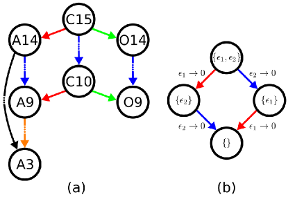
Figure 3: (a) The Hasse diagram of key reduced models for the Wnt system. The nodes (models) are labeled by “A” for accumulation, “O” for oscillation, “C” for combined, as well as the number of parameters each model contains. The black line represents the original sequence of reduced accumulation models and the blue line represents the new sequence with parameter limits reordered to match those in the oscillation models. The central, blue arrow shows that the original model can be reduced to the supremal model using the same set of limits used to arrive at A9 and O9. Details about the model equations and sequence of limits can be found in the supplemental material. (b) A general example of the diamond property. Consider a model with $N$ parameters containing two parameters $\epsilon_{1}$ and $\epsilon_{2}$. The diamond property states that the order in which parameters can be removed commutes. The same model with $N-2$ parameters can be reached by first taking either $\epsilon_{1}$ or $\epsilon_{2}$ to zero, and then taking the other to zero. The diamond property is used to reorder the limits of a sequence, to build a supremal model.

The MBAM reductions are not black boxes. Although the reduced models do abstract away many specific details, they retain vestiges of the full mechanisms, analogous to the SI and IR models in our epidemiology example. To relate these behaviors, we now seek the supremum of these two minimal representations. However, unlike the simple example, the minimal Wnt models contain partially overlapping combinations of parameters, so the construction is non-trivial.

Each reduction can be rewritten as a single parameter taken to zero. For example, consider an equilibrium approximation, i.e., $c_{f},c_{b}\rightarrow\infty$. This can be rewritten as a time constant going to zero $\tau_{f}=1/c_{f}\rightarrow 0$ and a nonzero equilibrium constant $K_{D}=c_{b}/c_{f}$. This form, however, is not unique as we could also have chosen $\tau_{b}=1/c_{b}\rightarrow 0$. For all equilibrium approximations we adopt the first as a standard form.

Next, we observe that the same reduced models could be derived by applying the same approximations in different orders. Commuting the order of reductions creates a diamond motif in the Hasse diagram, as in Fig. 3b. Because of the ambiguity in how reductions are labeled, consecutive limits including the same parameters can obscure this commutation relation. For example, consider the consecutive limits of an equilibrium approximation ($c_{bGA}\rightarrow\infty$, $c_{fGA}\rightarrow\infty$ with $c_{bGA}/c_{fGA}$ constant and finite) followed by an irreversible approximation ($c_{bGA}/c_{fGA}\rightarrow 0$, $c_{fAL}\rightarrow\infty$). Reparameterizing as $\epsilon_{1}=1/c_{fGA}$, $\epsilon_{2}=1/c_{fAL}$, and $\phi=c_{fAL}c_{bGA}/c_{fGA}$ makes the diamond property apparent. The two limits of the diamond property can now be written as $\epsilon_{1}\rightarrow 0$ and $\epsilon_{2}\rightarrow 0$.

Writing all of the reductions in a standard form allows us to identify the approximations common to both reduced models. Applying these common approximations to the original full model constructs the supremal model, as illustrated by the blue line connecting C15 to C10 in Fig. 3. This process motivates a general algorithm for finding supremal models, and is given below.

1. Define the hypothesis space by selecting a complex, multiparameter model to describe all desired behaviors.

2. Perform MBAM to find reduced models that minimally describe each behavior.

3. Reparameterize the models to detangle any conflated limits and find the approximations common to the both reduced models.

4. Apply those common approximations to the original, full model to obtain the supremal model.

Each of these steps is illustrated in Fig. 3. The original hypothesis space is represented by C15 (step 1). Models A3 and O9 minimally describe the accumulation and oscillation behaviors, respectively (step 2). Using the diamond property, illustrated in Fig. 3b, we reparameterize and find the approximations common to each reduced model, represented by the blue arrows (step 3). Applying these common approximations to C15 gives the supremal model, C10 (step 4). This process is described in more detail in the supplementary material, including a discussion on fitting the supremal model parameters and application to the Wnt model. Additionally, the supplemental material presents a second algorithm that exploits a general duality inherent in POSets.

Since the supremum has more parameters than either of the reduced models, the original data sets cannot individually constrain all of the supremal parameters. However, since each parameter is constrained by one data set of the other (e.g., $SA$ is constrained by the accumulation data but not eh oscillation data), fitting the supremal model to both data sets simultaneously does identify each parameter. By including both the feedback loop and external control, and their associated parameters, the supremum enables the accumulation and oscillation phenomena, as well as additional behaviors neither A14 nor O14 can produce. Fig. 2b demonstrates one such example, the “interrupted” behavior, in which the external control modulates the phase of the oscillation. Regular oscillatory behavior in the Wnt pathway is well-known in vivo from the segmentation clock in vertebrate embryos along the anterior-posterior axis to establish, for example, the repeating pattern of vertebrae and ribs Pourquie (2003). These regular oscillations can have their period and phase modified, stopped, or restarted through manipulation of “dorsalizing” or “ventralizing” molecular regulators, much like the interrupted behavior we see in the supremal model Riedel-Kruse et al. (2007); Gibb et al. (2009); Goldbeter and Pourquié (2008); Gomez et al. (2008); Rui et al. (2007). To validate our model, we apply MBAM to the full model using data for the interrupted regime. This reduction gives the supremal model constructed by our algorithm, indicating that the supremum is the model that would have been selected had observations been available for this behavior.

The supremum principle shows promise for transferring predictability to truly new domains. For example, the SI and IR models fail in the intermediate regime, and the accumulation and oscillation models fail in the interrupted regime, but the supremal models in each case are able to embrace all three behaviors. It does this by including key modeling elements (e.g., feedback and external control) that are missing from the reduced models. Since the supremal model combines distinct modeling elements, it enables new behaviors in regimes in which those modeling elements are all necessary. With a different starting model, couched in a different hypothesis space, the supremal model will be different, but it will still transfer according to the given hypothesis. This is more than the simple generalization of, e.g., multi-task learning (MTL) Caruana (1997). Supremal models apply in a more global way; they aim to improve the transferability to data in a completely new regime.

Classical psychological theories use geometric constructions to represent analogical relationships. Most notably, in the parallelogram model Rumelhart and Abrahamson (1973), an analogy such as man:king::woman:queen is represented as four corners of a parallelogram with analogical relationships forming parallel sides Peterson et al. (2020). Such constructions are widespread in AI applications ranging from recommender systems Musto (2010) to natural language processing Reid and Katz (2018). The key property, however, is the topological relationship between analogous elements Gentner (1983) that for parallelograms form the same diamond motif as in Fig. 3. The analogical relationships among words are the same as those between reduced models. Kings are subsets of men just as reduced models are restricted cases of more general models, and classifications based on royalty analogize across genders just as approximations transfer across models. Thus, the supremum construction identifies the mathematical “analogies” between models by teasing out the common mechanisms or analogous reductions (see the colored arrows in Fig. 3). The approximations in linking model C15 to model C10 are the same as those connecting model A14 to model A9, i.e., C15:C10::A14:A9. The colored arrows indicate the many other possible analogies that could be drawn among the models.

The supremum principle is applicable to any hierarchical family of models, and so there are some inherent limitations and potential extensions. First, the algorithm we present here is specific to hierarchies generated by MBAM, but future work could consider other families. Next, the result depends on the hierarchy one uses, for example, our Wnt study used the hierarchy generated by the model of Jensen et al. Jensen et al. (2010). Given different hierarchies, supremal models are a principled way of reasoning about the implications of those hypothesis. Future work may use supremal models to guide experimental design for hypothesis testing or parameter estimation. Finally, one could consider models that are derived independently of a hierarchical family. Future work could explore how to most naturally embed such models within a hierarchy to enable transferability.

Beyond the appeal of elegant, simplified models, we expect supremal models to be of broad practical use; for example, in systems that need a controller to move between two behavioral states, but is difficult to fully model and a reduced model is needed. Such systems include shifting from diseased to healthy states in medical contexts, failing to stable power grids in electrical engineering, ductile to brittle structures in material science, and collapsed to restored resources in ecosystem-based management. Supremal models are also designed for maximal simplicity while retaining some transferability, i.e., attempting to predict in regimes not yet examined, such as in climate modeling, prosperous non-growth-based economics, and human behavior during a pandemic. Practitioners from a wide variety of fields will find supremum modeling a powerful addition to their toolboxes.

This work was supported by the US National Science Foundation under Award NSF-1753357 (CP, CA, MKT), CMMT-1834332 (CP, MKT), and EPCN-1710727 (CA, MKT). We thank Sean Warnick, Kolten Barfuss, and Alex Stankovic for helpful conversations. We thank Ben Francis, Dan Karls, Ellad Tadmor, and Ryan Elliott and two anonymous reviewers for comments on the manuscript.

References

- Baxter (2000) J. Baxter, Journal of Artificial Intelligence Research 12, 149 (2000).
- Weiss et al. (2016) K. Weiss, T. M. Khoshgoftaar, and D. Wang, Journal of Big Data 3, 9 (2016).
- (3) R. W. Batterman, The Devil in the Details: Asymptotic Reasoning in Explanation, Reduction, and Emergence (Oxford University Press) google-Books-ID: EiIM5koj_J0C.
- Brown and Sethna (2003) K. S. Brown and J. P. Sethna, Physical Review E 68, 021904 (2003).
- Brown et al. (2004) K. S. Brown, C. C. Hill, G. A. Calero, C. R. Myers, K. H. Lee, J. P. Sethna, and R. A. Cerione, Physical Biology 1, 184 (2004).
- Waterfall et al. (2006) J. J. Waterfall, F. P. Casey, R. N. Gutenkunst, K. S. Brown, C. R. Myers, P. W. Brouwer, V. Elser, and J. P. Sethna, Physical Review Letters 97, 150601 (2006).
- Machta et al. (2013) B. B. Machta, R. Chachra, M. K. Transtrum, and J. P. Sethna, Science 342, 604 (2013).
- Amari and Nagaoka (2007) S.-i. Amari and H. Nagaoka, Methods of information geometry, Vol. 191 (American Mathematical Soc., 2007).
- Transtrum et al. (2010) M. K. Transtrum, B. B. Machta, and J. P. Sethna, Phys. Rev. Lett. 104, 060201 (2010).
- LaMont and Wiggins (2019) C. H. LaMont and P. A. Wiggins, Physical Review E 99, 052140 (2019).
- Quinn et al. (2019) K. N. Quinn, H. Wilber, A. Townsend, and J. P. Sethna, Physical Review Letters 122, 158302 (2019).
- Transtrum et al. (2011a) M. K. Transtrum, B. B. Machta, and J. P. Sethna, Physical Review E 83, 036701 (2011a).
- Lake et al. (2017) B. M. Lake, T. D. Ullman, J. B. Tenenbaum, and S. J. Gershman, Behavioral and Brain Sciences 40, e253 (2017).
- Webb et al. (2020) T. Webb, Z. Dulberg, S. Frankland, A. Petrov, R. O’Reilly, and J. Cohen, in Proceedings of the 37th International Conference on Machine Learning, Proceedings of Machine Learning Research, Vol. 119, edited by H. D. III and A. Singh (PMLR, 2020) pp. 10136–10146.
- Brouwer and Eisenberg (2018) A. F. Brouwer and M. C. Eisenberg, arXiv:1802.05641 [math] (2018), arXiv: 1802.05641.
- Transtrum and Qiu (2014) M. K. Transtrum and P. Qiu, Physical Review Letters 113, 098701 (2014).
- Transtrum et al. (2015) M. K. Transtrum, B. B. Machta, K. S. Brown, B. C. Daniels, C. R. Myers, and J. P. Sethna, The Journal of chemical physics 143, 07B201_1 (2015).
- Note (1) Although this approximation is constructed by taking , it does not require the “true” value of to be small. Rather, the role of the recovery mechanism can be compressed into a simpler model with an effective infection rate, similar to the effective electron mass in a condensed matter system.
- Goentoro and Kirschner (2009) L. Goentoro and M. W. Kirschner, Molecular Cell 36, 872 (2009).
- Jensen et al. (2010) P. B. Jensen, L. Pedersen, S. Krishna, and M. H. Jensen, Biophysical Journal 98, 943 (2010).
- Riedel-Kruse et al. (2007) I. H. Riedel-Kruse, C. Müller, and A. C. Oates, Science 317, 1911 (2007).
- Gibb et al. (2009) S. Gibb, A. Zagorska, K. Melton, G. Tenin, I. Vacca, P. Trainor, M. Maroto, and J. K. Dale, Developmental Biology 330, 21 (2009).
- Goldbeter and Pourquié (2008) A. Goldbeter and O. Pourquié, Journal of Theoretical Biology 252, 574 (2008).
- Gomez et al. (2008) C. Gomez, E. M. Özbudak, J. Wunderlich, D. Baumann, J. Lewis, and O. Pourquié, Nature 454, 335 (2008).
- Rui et al. (2007) Y. Rui, Z. Xu, B. Xiong, Y. Cao, S. Lin, M. Zhang, S. C. Chan, W. Luo, Y. Han, Z. Lu, Z. Ye, H. M. Zhou, J. Han, A. Meng, and S. C. Lin, Developmental Cell 13, 268 (2007).
- Transtrum et al. (2014) M. K. Transtrum, G. Hart, and P. Qiu, CoRR (2014), arXiv:1409.6203 [physics.data-an] .
- Svenda et al. (2021) V. G. Svenda, M. K. Transtrum, B. L. Francis, A. T. Saric, and A. M. Stankovic, IEEE Transactions on Power Systems (2021).
- Sarić et al. (2020) A. T. Sarić, A. A. Sarić, M. K. Transtrum, and A. M. Stanković, IEEE Transactions on Power Systems 36, 2390 (2020).
- Francis et al. (2019) B. L. Francis, J. R. Nuttall, M. K. Transtrum, A. T. Sarić, and A. M. Stanković, in 2019 North American Power Symposium (NAPS) (IEEE, 2019) pp. 1–6.
- Transtrum et al. (2016) M. K. Transtrum, A. T. Sarić, and A. M. Stanković, IEEE Transactions on Power Systems 32, 2243 (2016).
- Jeong et al. (2018) J. E. Jeong, Q. Zhuang, M. K. Transtrum, E. Zhou, and P. Qiu, Quantitative Biology 6, 287 (2018).
- Transtrum and Qiu (2016) M. K. Transtrum and P. Qiu, PLoS computational biology 12, e1004915 (2016).
- Mannakee et al. (2016) B. K. Mannakee, A. P. Ragsdale, M. K. Transtrum, and R. N. Gutenkunst, in Uncertainty in Biology (Springer, 2016) pp. 271–299.
- Kurniawan et al. (2021) Y. Kurniawan, C. L. Petrie, K. J. Williams, M. K. Transtrum, E. B. Tadmor, R. S. Elliott, D. S. Karls, and M. Wen, arXiv preprint arXiv:2112.10851 (2021).
- Marschmann et al. (2019) G. L. Marschmann, H. Pagel, P. Kügler, and T. Streck, Environmental Modelling & Software 122, 104518 (2019).
- Nikšić et al. (2017) T. Nikšić, M. Imbrišak, and D. Vretenar, Physical Review C 95, 054304 (2017).
- Rasband (2021) J. Rasband, Two Reduced Models of Nerve Behavior, Bachelor’s thesis, Brigham Young University (2021).
- Paré et al. (2019) P. E. Paré, D. Grimsman, A. T. Wilson, M. K. Transtrum, and S. Warnick, IEEE Transactions on Automatic Control 64, 4796 (2019).
- Gerach et al. (2019) T. Gerach, D. Weiß, O. Dössel, and A. Loewe, in 2019 Computing in Cardiology (CinC) (IEEE, 2019) p. 1.
- Lombardo and Rappel (2017) D. M. Lombardo and W.-J. Rappel, Chaos: An Interdisciplinary Journal of Nonlinear Science 27, 093914 (2017).
- Paré et al. (2015) P. E. Paré, A. T. Wilson, M. K. Transtrum, and S. C. Warnick, in 2015 American Control Conference (IEEE, 2015) pp. 1989–1994.
- Lee et al. (2003) E. Lee, A. Salic, R. Krüger, R. Heinrich, and M. W. Kirschner, PLOS Biology 1, e10 (2003).
- Ji et al. (2019) L. Ji, B. Lu, R. Zamponi, O. Charlat, R. Aversa, Z. Yang, F. Sigoillot, X. Zhu, T. Hu, J. S. Reece-Hoyes, C. Russ, G. Michaud, J. S. Tchorz, X. Jiang, and F. Cong, Nature Communications 10, 4184 (2019).
- Gutenkunst et al. (2007) R. N. Gutenkunst, J. J. Waterfall, F. P. Casey, K. S. Brown, C. R. Myers, and J. P. Sethna, PLOS Computational Biology 3, e189 (2007).
- Transtrum et al. (2011b) M. K. Transtrum, B. B. Machta, and J. P. Sethna, Physical Review E 83, 036701 (2011b).
- Pourquie (2003) O. Pourquie, Science 301, 328 (2003).
- Caruana (1997) R. Caruana, Machine Learning 28, 41 (1997).
- Rumelhart and Abrahamson (1973) D. E. Rumelhart and A. A. Abrahamson, Cognitive Psychology 5, 1 (1973).
- Peterson et al. (2020) J. C. Peterson, D. Chen, and T. L. Griffiths, Cognition 205, 104440 (2020).
- Musto (2010) C. Musto, in Proceedings of the fourth ACM conference on Recommender systems (2010) pp. 361–364.
- Reid and Katz (2018) J. N. Reid and A. N. Katz, Metaphor and Symbol 33, 280 (2018).
- Gentner (1983) D. Gentner, Cognitive Science 7, 155 (1983).