Thermodynamics of an Ising-like $XXZ$ chain in a longitudinal magnetic field in the framework of the Quantum Transfer Matrix approach

P.Β N.Β Bibikov
(Russian State Hydrometeorological University, Saint-Petersburg, Russia)
Abstract

Taking the Ising chain as a reference model we have derived a perturbative expression for the free energy density of the Heisenberg-Ising chain with strong easy-axis anisotropy. All calculations are performed on the ground of the Quantum Transfer Matrix approach. The obtained result agrees with the direct high-temperature expansion. It also agrees with the low-temperature cluster expansion in the special subregime when quantum fluctuations are weak against thermodynamical ones.


1 Introduction

One of the basic models of one-dimensional quantum magnetism is the $XXZ$ spin chain in a longitudinal magnetic field $h$ [1]. It corresponds to the Hamiltonian

$$\hat{H}=\sum_{n=1}^{N}\Big{[}\frac{J}{2}\Big{(}{\bf S}^{+}_{n}{\bf S}^{-}_{n+1}+{\bf S}^{-}_{n}{\bf S}^{+}_{n+1}\Big{)}+J_{z}\Big{(}{\bf S}^{z}_{n}{\bf S}^{z}_{n+1}-\frac{1}{4}I\Big{)}-h{\bf S}_{n}^{z}\Big{]},\qquad h\geq 0,$$ (1)

where ${\bf S}_{n}^{z}$ and ${\bf S}_{n}^{\pm}={\bf S}_{n}^{x}\pm i{\bf S}_{n}^{y}$ are the usual spin-1/2 operators. At $J=0$ the model (1) reduces to the Ising chain solvable by a rather simple machinery [2].

Being purely classical ($[{\bf S}_{m}^{z},{\bf S}_{n}^{z}]=0$) the Ising model is rather poor (for example the Ising magnons are dispersionless). Nevertheless it was suggested for a number of magnetic compounds [3, 4, 5]. However since the condition $J=0$ does not follow from any symmetry it is natural to suppose that a more adequate model for these compounds is the Ising-like chain described by Hamiltonian (1) supplemented by the condition

$$\Delta\equiv\frac{J_{z}}{J}\gg 1.$$ (2)

The model (1), (2) was also suggested for some real compounds [6, 7]. Being quantum it has a more rich physical behavior and at the same time should allow a perturbative treatment around the Ising model.

In the last two decades a new machinery for evaluation of thermodynamics of quantum spin chains was suggested basing on the Quantum Transfer Matrix (QTM) approach (see reviews [8, 9] and references therein). The latter has two main stages. Within the former one a system of integral equations on specially introduced auxiliary functions is derived. Within the latter one an integral representations for the free energy density

$$f(T,h)=-\frac{1}{\beta}\lim_{N\rightarrow\infty}\frac{1}{N}\ln{Z_{N}(T,h)},$$ (3)

(as usual $Z_{N}(T,h)$ is the partition function and $\beta\equiv 1/T$) and correlation functions are obtained in this framework.

In the Ising $J=0$ case the corresponding free energy density has the form

fI​s​(T,h)=e0​(h)βˆ’1β​ln⁑(1+eβˆ’Ξ²β€‹h+(1βˆ’eβˆ’Ξ²β€‹h)2+4​eβ​(Jzβˆ’h)2),superscriptπ‘“πΌπ‘ π‘‡β„Žsubscript𝑒0β„Ž1𝛽1superscripteπ›½β„Žsuperscript1superscripteπ›½β„Ž24superscripte𝛽subscriptπ½π‘§β„Ž2f^{Is}(T,h)=e_{0}(h)-\frac{1}{\beta}\ln{\left(\frac{1+{\rm e}^{-\beta h}+\sqrt{(1-{\rm e}^{-\beta h})^{2}+4{\rm e}^{\beta(J_{z}-h)}}}{2}\right)}, (4)

where

$$e_{0}(h)=-\frac{h}{2}$$ (5)

is the ground state energy density. Formula (4) readily follows from the representation [2]

fI​s​(T,h)=βˆ’1β​ln⁑Λ+​(Ξ²,h),superscriptπ‘“πΌπ‘ π‘‡β„Ž1𝛽subscriptΞ›π›½β„Žf^{Is}(T,h)=-\frac{1}{\beta}\ln{\Lambda_{+}(\beta,h)}, (6)

where

$$\Lambda_{\pm}(\beta,h)=\cosh{\frac{\beta h}{2}}\pm\sqrt{\sinh^{2}{\frac{\beta h}{2}}+{\rm e}^{\beta J_{z}}},$$ (7)

are eigenvalues of the special transfer matrix

$$T=\left(\begin{array}[]{cc}{\rm e}^{\beta h/2}&{\rm e}^{\beta J/2}\\ {\rm e}^{\beta J/2}&{\rm e}^{-\beta h/2}\end{array}\right),$$ (8)

related to the Hamiltonian (1) at $J=0$. As it has been mentioned in [10] formula (4) also may be obtained within the approach of [8, 9].

In the present paper we extend the result of [10] studying the model (1), (2) at the vicinity of the Ising point in the first two perturbation orders. The paper is organized as follows. In Sect. 2 following [10] we introduce the basic auxiliary functions and corresponding integral equations. We use however rather different notations which seem us to be more convenient for our treatment. We also show how to account singularities in the kernels of the integral equations. In Sect. 3 we extract the auxiliary functions related to the Ising model [10] and reduce the integral equations to the form convenient for perturbative expansion. In Sect. 4 we calculate the first two terms of the perturbation expansion and evaluate the corresponding correction to the free energy density. In Sect. 5 treating the high-temperature regime

$$h,|J_{z}|,|J|\ll k_{B}T\Longleftrightarrow\beta\cdot\max{(h,|J_{z}|,|J|)}\ll 1,$$ (9)

we compare the first order terms of the high-temperature expansion which follows from the obtained formula for $f(T,h)$ with the one directly related to (3). Showing that both approaches give the same result we confirm the effectiveness of the approach [8, 9] at high temperatures [11]. In Sect. 6 we study the low-temperature regime in the phase related to the ferromagnetically polarized ground state

$$|\emptyset\rangle=\dots\otimes|\uparrow\rangle\otimes|\uparrow\rangle\otimes|\uparrow\rangle\otimes\dots,\qquad{\bf S}^{z}|\uparrow\rangle=\frac{1}{2}|\uparrow\rangle,$$ (10)

and non-zero magnon gap energy [12]

$$E_{gap}=h-J_{z}-|J|>0.$$ (11)

Comparing the calculated peturbative result with the one obtained previously by the low-temperature cluster expansion [12] we show that in the extreme low-temperature subregime

$$k_{B}T\ll\frac{E_{width}}{2},$$ (12)

where

$$E_{width}=2|J|,$$ (13)

is the magnon band width, the both approaches totally disagree. However they give similar results in the scaled low-temperature subregime

$$\frac{E_{width}}{2}\ll k_{B}T\ll E_{gap}+\frac{E_{width}}{2}.$$ (14)

If one suggest that low-temperature quantum fluctuations arise from transitions within the magnon band then the associated fluctuation of energy should be $E_{width}$. Hence the scaled low-temperature regime corresponds to weakness of quantum fluctuations against thermodynamical ones.

2 Foundations of the ${\mathfrak{b}}_{+}$-${\mathfrak{b}}_{-}$-formalism

Following [10] (however with unconventional notations $\mathfrak{b}_{+}(x)$ and $\mathfrak{b}_{-}(x)$ instead of $\mathfrak{b}(x)$ and $\bar{\mathfrak{b}}(x)$) we suggest the following system of equations

$$\ln{\mathfrak{b}_{\pm}}(x)+\int_{-\pi/2}^{\pi/2}dy\Big{(}\kappa_{\mp}(x-y)\ln{\mathfrak{B}_{\mp}}(y)-\kappa(x-y)\ln{\mathfrak{B}_{\pm}}(y)\Big{)}=\mp\frac{\beta h}{2}-J_{z}\beta c(x),$$ (15)

where

$$\mathfrak{B}_{\pm}(x)=1+\mathfrak{b}_{\pm}(x),$$ (16)

and the $T=\infty$ condition

$$\lim_{T\rightarrow\infty}{\mathfrak{b}_{\pm}}(x,T,h)=1.$$ (17)

Here

$\displaystyle d(x)=\sum_{m=-\infty}^{\infty}\frac{{\rm e}^{2imx}}{{\rm ch}{(\eta m)}},\qquad c(x)=\frac{d(x)\tanh{\eta}}{2},\qquad\kappa(x)=\frac{1}{\pi}\sum_{m=-\infty}^{\infty}\frac{{\rm e}^{2imx}}{1+{\rm e}^{2\eta|m|}},$
$\displaystyle\kappa_{\pm}(x)=\kappa(x\pm i\eta\mp i\epsilon)=\frac{1}{\pi}\sum_{m=-\infty}^{\infty}\frac{{\rm e}^{\mp 2(\eta-\epsilon)m}}{1+{\rm e}^{2\eta|m|}}{\rm e}^{2imx},$ (18)

and it is assumed that

$$\cosh{\eta}=\frac{J_{z}}{J},\qquad\eta>0.$$ (19)

Functions $\kappa_{\pm}(x)$ have singular parts. In order to extract them we shall use the following extended representations

$\displaystyle\kappa_{+}(x)=\frac{1}{\pi}\Big{[}\frac{1}{2}+\sum_{m=1}^{\infty}\frac{{\rm e}^{2(ix-\eta)m}}{1+{\rm e}^{2\eta m}}+\sum_{m=-\infty}^{-1}\Big{(}1-\frac{1}{1+{\rm e}^{2\eta|m|}}\Big{)}{\rm e}^{2(ix+\epsilon)m}\Big{]},$
$\displaystyle\kappa_{-}(x)=\frac{1}{\pi}\Big{[}\frac{1}{2}+\sum_{m=1}^{\infty}\Big{(}1-\frac{1}{1+{\rm e}^{2\eta m}}\Big{)}{\rm e}^{2(ix-\epsilon)m}+\sum_{m=-\infty}^{-1}\frac{{\rm e}^{2(ix+\eta)m}}{1+{\rm e}^{2\eta|m|}}\Big{]}.$ (20)

Hence for a function

$$\varphi(x)=\varphi^{(0)}+\varphi^{(+)}(x)+\varphi^{(-)}(x),$$ (21)

where $\varphi^{(0)}$ is a number and

$$\varphi^{(+)}(x)=\sum_{m=1}^{\infty}\varphi^{(m)}{\rm e}^{2imx},\qquad\varphi^{(-)}(x)=\sum_{m=1}^{\infty}\varphi^{(-m)}{\rm e}^{-2imx},$$ (22)

one has

$$\int_{-\pi/2}^{\pi/2}\kappa_{\pm}(x-y)\varphi(y)dy=\frac{\varphi^{(0)}}{2}+\varphi^{(\mp)}(x)+\int_{-\pi/2}^{\pi/2}\tilde{\kappa}_{\pm}(x-y)(\varphi^{(+)}(y)+\varphi^{(+)}(y))dy,$$ (23)

where

$\displaystyle\tilde{\kappa}_{+}(x)=\frac{1}{\pi}\left(\sum_{m=1}^{\infty}\frac{{\rm e}^{2(ix-\eta)m}}{1+{\rm e}^{2\eta m}}-\sum_{m=-\infty}^{-1}\frac{{\rm e}^{2ixm}}{1+{\rm e}^{2\eta|m|}}\right),$
$\displaystyle\tilde{\kappa}_{-}(x)=\frac{1}{\pi}\left(-\sum_{m=1}^{\infty}\frac{{\rm e}^{2ixm}}{1+{\rm e}^{2\eta m}}+\sum_{m=-\infty}^{-1}\frac{{\rm e}^{2(ix+\eta)m}}{1+{\rm e}^{2\eta|m|}}\right).$ (24)

With the use of the auxiliary functions ${\mathfrak{B}}_{\pm}(x)$ the free energy density (3) may be represented by the formula [10]

$$f(T,h)=-\frac{J_{z}\tanh{\eta}}{2}\sum_{m=-\infty}^{\infty}\frac{{\rm e}^{-\eta|m|}}{\cosh{(\eta m)}}-\frac{1}{2\pi\beta}\int_{-\pi/2}^{\pi/2}dxd(x)\ln{({\mathfrak{B}}_{+}(x){\mathfrak{B}}_{-}(x))}.$$ (25)

3 The Ising solution and around

At the Ising point

$$J=0\Longleftrightarrow\eta=\infty,$$ (26)

one has from (18) and (24)

dI​s​(x)=1,cI​s​(x)=12,ΞΊI​s​(x)=12​π,ΞΊ~Β±I​s​(x)=0,formulae-sequencesuperscript𝑑𝐼𝑠π‘₯1formulae-sequencesuperscript𝑐𝐼𝑠π‘₯12formulae-sequencesuperscriptπœ…πΌπ‘ π‘₯12πœ‹subscriptsuperscript~πœ…πΌπ‘ plus-or-minusπ‘₯0d^{Is}(x)=1,\qquad c^{Is}(x)=\frac{1}{2},\qquad\kappa^{Is}(x)=\frac{1}{2\pi},\qquad\tilde{\kappa}^{Is}_{\pm}(x)=0, (27)

so the right side of (15) does not depend on $x$ and a substitution

π”ŸΒ±β€‹(x)βŸΆπ”ŸΒ±I​s,𝔅±​(x)βŸΆπ”…Β±I​s=1+π”ŸΒ±I​sformulae-sequence⟢subscriptπ”Ÿplus-or-minusπ‘₯superscriptsubscriptπ”Ÿplus-or-minusπΌπ‘ βŸΆsubscript𝔅plus-or-minusπ‘₯superscriptsubscript𝔅plus-or-minus𝐼𝑠1superscriptsubscriptπ”Ÿplus-or-minus𝐼𝑠{\mathfrak{b}}_{\pm}(x)\longrightarrow{\mathfrak{b}}_{\pm}^{Is},\qquad{\mathfrak{B}}_{\pm}(x)\longrightarrow{\mathfrak{B}}_{\pm}^{Is}=1+{\mathfrak{b}}_{\pm}^{Is} (28)

yields the following system of algebraic equations

$$\ln{\mathfrak{b}_{\pm}^{Is}}+\frac{\ln{\mathfrak{B}_{\mp}^{Is}}-\ln{\mathfrak{B}_{\pm}^{Is}}}{2}=\mp\frac{\beta h}{2}-\frac{J_{z}\beta}{2}\Longleftrightarrow({\mathfrak{b}}_{\pm}^{Is})^{2}\frac{1+{\mathfrak{b}}_{\mp}^{Is}}{1+{\mathfrak{b}}_{\pm}^{Is}}={\rm e}^{\beta(-J_{z}\mp h)},$$ (29)

or in an equivalent form

π”Ÿ+I​sβ€‹π”Ÿβˆ’I​s=eβˆ’Ξ²β€‹Jz,(π”ŸΒ±I​s)2+eβˆ’Ξ²β€‹Jzβ€‹π”ŸΒ±I​sπ”ŸΒ±I​s+1=eβ​(βˆ’Jzβˆ“h).formulae-sequencesuperscriptsubscriptπ”ŸπΌπ‘ superscriptsubscriptπ”ŸπΌπ‘ superscripte𝛽subscript𝐽𝑧superscriptsuperscriptsubscriptπ”Ÿplus-or-minus𝐼𝑠2superscripte𝛽subscript𝐽𝑧superscriptsubscriptπ”Ÿplus-or-minus𝐼𝑠superscriptsubscriptπ”Ÿplus-or-minus𝐼𝑠1superscripte𝛽minus-or-plussubscriptπ½π‘§β„Ž{\mathfrak{b}}_{+}^{Is}{\mathfrak{b}}_{-}^{Is}={\rm e}^{-\beta J_{z}},\qquad\frac{({\mathfrak{b}}_{\pm}^{Is})^{2}+{\rm e}^{-\beta J_{z}}{\mathfrak{b}}_{\pm}^{Is}}{{\mathfrak{b}}_{\pm}^{Is}+1}={\rm e}^{\beta(-J_{z}\mp h)}. (30)

At the same time formula (25) in the Ising case (26) reduces to

fI​s​(T,h)=βˆ’Jz2βˆ’12​β​ln⁑(𝔅+I​sβ€‹π”…βˆ’I​s).superscriptπ‘“πΌπ‘ π‘‡β„Žsubscript𝐽𝑧212𝛽subscriptsuperscript𝔅𝐼𝑠subscriptsuperscript𝔅𝐼𝑠f^{Is}(T,h)=-\frac{J_{z}}{2}-\frac{1}{2\beta}\ln{({\mathfrak{B}}^{Is}_{+}{\mathfrak{B}}^{Is}_{-})}. (31)

System (30), (17) has the single solution

$${\mathfrak{b}}_{\pm}^{Is}={\rm e}^{-\beta(J_{z}\pm h/2)}\Big{(}\sqrt{\sinh^{2}{\frac{\beta h}{2}}+{\rm e}^{\beta J_{z}}}\mp\sinh{\frac{\beta h}{2}}\Big{)}.$$ (32)

According to (16) and (30)

𝔅+I​sβ€‹π”…βˆ’I​s=1+eβˆ’Ξ²β€‹Jz+π”Ÿ+I​s+π”Ÿβˆ’I​s,superscriptsubscript𝔅𝐼𝑠superscriptsubscript𝔅𝐼𝑠1superscripte𝛽subscript𝐽𝑧superscriptsubscriptπ”ŸπΌπ‘ superscriptsubscriptπ”ŸπΌπ‘ {\mathfrak{B}}_{+}^{Is}{\mathfrak{B}}_{-}^{Is}=1+{\rm e}^{-\beta J_{z}}+{\mathfrak{b}}_{+}^{Is}+{\mathfrak{b}}_{-}^{Is}, (33)

so a substitution of (32) into (33) gives

$\displaystyle{\mathfrak{B}}_{+}^{Is}{\mathfrak{B}}_{-}^{Is}=1+{\rm e}^{-\beta J_{z}}\Big{(}2\cosh{\frac{\beta h}{2}}\cdot\sqrt{\sinh^{2}{\frac{\beta h}{2}}+{\rm e}^{\beta J_{z}}}+\cosh^{2}{\frac{\beta h}{2}}+\sinh^{2}{\frac{\beta h}{2}}\Big{)}$
$\displaystyle={\rm e}^{-\beta J_{z}}\Big{(}\cosh{\frac{\beta h}{2}}+\sqrt{\sinh^{2}{\frac{\beta h}{2}}+{\rm e}^{\beta J_{z}}}\Big{)}^{2}.$ (34)

So (4) really follows from (31) and (34) [10].

Let us now extract the Ising solution taking

π”ŸΒ±β€‹(x)=π”ŸΒ±I​s+π”Ÿ~±​(x),f​(T,h)=fI​s​(T,h)+f~​(T,h),formulae-sequencesubscriptπ”Ÿplus-or-minusπ‘₯superscriptsubscriptπ”Ÿplus-or-minus𝐼𝑠subscript~π”Ÿplus-or-minusπ‘₯π‘“π‘‡β„Žsuperscriptπ‘“πΌπ‘ π‘‡β„Ž~π‘“π‘‡β„Ž{\mathfrak{b}}_{\pm}(x)={\mathfrak{b}}_{\pm}^{Is}+{\tilde{\mathfrak{b}}}_{\pm}(x),\qquad f(T,h)=f^{Is}(T,h)+\tilde{f}(T,h), (35)

as well as

d​(x)=dI​s+d~​(x),c​(x)=cI​s+c~​(x),κ​(x)=ΞΊI​s+ΞΊ~​(x),formulae-sequence𝑑π‘₯superscript𝑑𝐼𝑠~𝑑π‘₯formulae-sequence𝑐π‘₯superscript𝑐𝐼𝑠~𝑐π‘₯πœ…π‘₯superscriptπœ…πΌπ‘ ~πœ…π‘₯d(x)=d^{Is}+\tilde{d}(x),\qquad c(x)=c^{Is}+\tilde{c}(x),\qquad\kappa(x)=\kappa^{Is}+\tilde{\kappa}(x), (36)

where according to (18), (27) and (36)

$\displaystyle\tilde{d}(x)=2\sum_{m=1}^{\infty}\frac{\cos{2mx}}{\cosh{\eta m}},\qquad\tilde{c}(x)=\tanh\eta\sum_{m=1}^{\infty}\frac{\cos{2mx}}{{\rm ch}{(\eta m)}}-\frac{{\rm e}^{-2\eta}}{1+{\rm e}^{-2\eta}},$
$\displaystyle\tilde{\kappa}(x)=\frac{2}{\pi}\sum_{m=1}^{\infty}\frac{\cos{2mx}}{1+{\rm e}^{2\eta m}}.$ (37)

From (24) and (37) readily follows that

$$\int_{-\pi/2}^{\pi/2}\tilde{d}(x)dx=\int_{-\pi/2}^{\pi/2}\tilde{\kappa}(x)dx=\int_{-\pi/2}^{\pi/2}\tilde{\kappa}_{\pm}(x)dx=0.$$ (38)

Using now (35)-(38) one may reduce (15) and (25) to the forms

$\displaystyle\ln{\Big{(}1+\frac{\tilde{\mathfrak{b}}_{\pm}(x)}{\mathfrak{b}_{\pm}^{Is}}\Big{)}}+\int_{-\pi/2}^{\pi/2}dy\Big{[}\kappa_{\mp}(x-y)\ln{\Big{(}1+\frac{\tilde{\mathfrak{b}}_{\mp}(y)}{\mathfrak{B}_{\mp}^{Is}}\Big{)}}$
$\displaystyle-\kappa(x-y)\ln{\Big{(}1+\frac{\tilde{\mathfrak{b}}_{\pm}(y)}{\mathfrak{B}_{\pm}^{Is}}\Big{)}}\Big{]}=-J_{z}\beta\tilde{c}(x),$ (39)

and

$\displaystyle\tilde{f}(T,h)=J_{z}\Big{(}\frac{1-\tanh{\eta}}{2}-2\tanh{\eta}\sum_{m=1}^{\infty}\frac{{\rm e}^{-2\eta m}}{1+{\rm e}^{-2\eta m}}\Big{)}$
$\displaystyle-\frac{1}{2\pi\beta}\int_{-\pi/2}^{\pi/2}dxd(x)\Big{[}\ln{\Big{(}1+\frac{\tilde{\mathfrak{b}}_{+}(x)}{\mathfrak{B}_{+}^{Is}}\Big{)}}+\ln{\Big{(}1+\frac{\tilde{\mathfrak{b}}_{-}(x)}{\mathfrak{B}_{-}^{Is}}\Big{)}}\Big{]},$ (40)

more convenient for the perturbative series expansion.

4 Series expansion near the Ising point

Suggesting the series expansions

$\displaystyle{\tilde{\mathfrak{b}}}_{\pm}(x)=\sum_{j=1}^{\infty}{\rm e}^{-\eta j}{\mathfrak{b}}_{\pm}^{(j)}(x),$ (41)
$\displaystyle\tilde{f}(T,h)=\sum_{j=1}^{\infty}{\rm e}^{-\eta j}f^{(j)}(T,h),$ (42)

and representing each ${\mathfrak{b}}_{\pm}^{(j)}(x)$ in the separated form (21)

$${\mathfrak{b}}_{\pm}^{(j)}(x)={\mathfrak{b}}_{\pm}^{(j;0)}+{\mathfrak{b}}_{\pm}^{(j;+)}(x)+{\mathfrak{b}}_{\pm}^{(j;-)}(x),$$ (43)

where

$${\mathfrak{b}}_{\pm}^{(j;+)}(x)=\sum_{m=1}^{\infty}{\mathfrak{b}}_{\pm}^{(j;2m)}{\rm e}^{2imx},\qquad{\mathfrak{b}}_{\pm}^{(j;-)}(x)=\sum_{m=1}^{\infty}{\mathfrak{b}}_{\pm}^{(j;-2m)}{\rm e}^{-2imx},$$ (44)

we shall calculate ${\mathfrak{b}}_{\pm}^{(j)}(x)$ and $f^{(j)}(T,h)$ for $j=1,2$. Since

$$\frac{1}{\Delta}\equiv\frac{1}{\cosh{\eta}}=2{\rm e}^{-\eta}+o({\rm e}^{-2\eta}),$$ (45)

formula

$$\tilde{f}(T,h)={\rm e}^{-\eta}f^{(1)}(T,h)+{\rm e}^{-2\eta}f^{(2)}(T,h)+o({\rm e}^{-2\eta}),$$ (46)

is equivalent to

$$\tilde{f}(T,h)=\frac{f^{(1)}(T,h)}{2\Delta}+\frac{f^{(2)}(T,h)}{4\Delta^{2}}+o\Big{(}\frac{1}{\Delta^{2}}\Big{)}.$$ (47)

For evaluation of the first two terms in the right sides of (41) and (42) we also need the expansions

$\displaystyle\tilde{c}(x)=2{\rm e}^{-\eta}\cos{2x}+(2\cos{4x}-1){\rm e}^{-2\eta}+o({\rm e}^{-2\eta}),$
$\displaystyle\tilde{\kappa}(x)=\frac{2{\rm e}^{-2\eta}}{\pi}\cos{2x}+o({\rm e}^{-2\eta}),$
$\displaystyle\tilde{\kappa}_{\pm}(x)=-\frac{{\rm e}^{2(\mp ix-\eta)}}{\pi}+o({\rm e}^{-2\eta}),$
$\displaystyle d(x)=1+4({\rm e}^{-\eta}\cos{2x}+{\rm e}^{-2\eta}\cos{4x})+o({\rm e}^{-2\eta}),$
$\displaystyle\frac{1-\tanh{\eta}}{2}-2\tanh{\eta}\sum_{m=1}^{\infty}\frac{{\rm e}^{-2\eta m}}{1+{\rm e}^{-2\eta m}}=-{\rm e}^{-2\eta}+o({\rm e}^{-2\eta}),$ (48)

which directly follow from (37) and (24).

Using (48) one readily gets in the order ${\rm e}^{-\eta}$

$$f^{(1)}(T,h)=-\frac{1}{2\pi\beta}\int_{-\pi/2}^{\pi/2}\Big{(}\frac{\mathfrak{b}_{+}^{(1)}(x)}{\mathfrak{B}_{+}^{Is}}+\frac{\mathfrak{b}_{-}^{(1)}(x)}{\mathfrak{B}_{-}^{Is}}\Big{)}dx=-\frac{1}{2\beta}\Big{(}\frac{\mathfrak{b}_{+}^{(1;0)}}{\mathfrak{B}_{+}^{Is}}+\frac{\mathfrak{b}_{-}^{(1;0)}}{\mathfrak{B}_{-}^{Is}}\Big{)},$$ (49)

and

$$\frac{\mathfrak{b}_{\pm}^{(1)}(x)}{\mathfrak{b}_{\pm}^{Is}}+\frac{\mathfrak{b}_{\mp}^{(1;\pm)}(x)}{\mathfrak{B}_{\mp}^{Is}}+\frac{1}{2\pi}\int_{-\pi/2}^{\pi/2}\Big{[}\frac{\mathfrak{b}_{\mp}^{(1)}(y)}{\mathfrak{B}_{\mp}^{Is}}-\frac{\mathfrak{b}_{\pm}^{(1)}(y)}{\mathfrak{B}_{\pm}^{Is}}\Big{]}dy=-2J_{z}\beta\cos{2x},$$ (50)

or in an expanded form

$\displaystyle\frac{\mathfrak{b}_{\pm}^{(1;0)}}{\mathfrak{b}_{\pm}^{Is}}+\frac{1}{2}\Big{[}\frac{\mathfrak{b}_{\mp}^{(1;0)}}{\mathfrak{B}_{\mp}^{Is}}-\frac{\mathfrak{b}_{\pm}^{(1;0)}}{\mathfrak{B}_{\pm}^{Is}}\Big{]}=0,$ (51)
π”Ÿ+(1;2)​(x)π”Ÿ+I​s+π”Ÿβˆ’(1;2)​(x)π”…βˆ’I​s=βˆ’Jz​β,π”Ÿ+(1;βˆ’2)​(x)π”Ÿ+I​s=βˆ’Jz​β,formulae-sequencesuperscriptsubscriptπ”Ÿ12π‘₯superscriptsubscriptπ”ŸπΌπ‘ superscriptsubscriptπ”Ÿ12π‘₯superscriptsubscript𝔅𝐼𝑠subscript𝐽𝑧𝛽superscriptsubscriptπ”Ÿ12π‘₯superscriptsubscriptπ”ŸπΌπ‘ subscript𝐽𝑧𝛽\displaystyle\frac{\mathfrak{b}_{+}^{(1;2)}(x)}{\mathfrak{b}_{+}^{Is}}+\frac{\mathfrak{b}_{-}^{(1;2)}(x)}{\mathfrak{B}_{-}^{Is}}=-J_{z}\beta,\qquad\frac{\mathfrak{b}_{+}^{(1;-2)}(x)}{\mathfrak{b}_{+}^{Is}}=-J_{z}\beta,
π”Ÿβˆ’(1;2)​(x)π”Ÿβˆ’I​s=βˆ’Jz​β,π”Ÿβˆ’(1;βˆ’2)​(x)π”Ÿβˆ’I​s+π”Ÿ+(1;βˆ’2)​(x)𝔅+I​s=βˆ’Jz​β.formulae-sequencesuperscriptsubscriptπ”Ÿ12π‘₯superscriptsubscriptπ”ŸπΌπ‘ subscript𝐽𝑧𝛽superscriptsubscriptπ”Ÿ12π‘₯superscriptsubscriptπ”ŸπΌπ‘ superscriptsubscriptπ”Ÿ12π‘₯superscriptsubscript𝔅𝐼𝑠subscript𝐽𝑧𝛽\displaystyle\frac{\mathfrak{b}_{-}^{(1;2)}(x)}{\mathfrak{b}_{-}^{Is}}=-J_{z}\beta,\qquad\frac{\mathfrak{b}_{-}^{(1;-2)}(x)}{\mathfrak{b}_{-}^{Is}}+\frac{\mathfrak{b}_{+}^{(1;-2)}(x)}{\mathfrak{B}_{+}^{Is}}=-J_{z}\beta. (52)

Representing homogeneous linear system (51) as

$$(2+\mathfrak{b}_{\pm}^{Is})t_{\pm}+\mathfrak{b}_{\pm}^{Is}t_{\mp}=0,\qquad t_{\pm}\equiv\frac{\mathfrak{b}_{\pm}^{Is}}{1+\mathfrak{b}_{\pm}^{Is}},$$ (53)

one readily concludes that its nontrivial solvability implies condition π”Ÿ+I​s+π”Ÿβˆ’I​s=βˆ’2superscriptsubscriptπ”ŸπΌπ‘ superscriptsubscriptπ”ŸπΌπ‘ 2\mathfrak{b}_{+}^{Is}+\mathfrak{b}_{-}^{Is}=-2 which can not be fulfilled because both $\mathfrak{b}_{\pm}^{Is}$ in (32) are positive. Hence (51) yields

$$\mathfrak{b}_{\pm}^{(1;0)}=0,$$ (54)

and according to (49) and (54)

$$f^{(1)}(T,h)=0.$$ (55)

The remaining system (52) gives

π”Ÿ+(1;2)=βˆ’Jzβ€‹Ξ²β€‹π”Ÿ+I​sπ”…βˆ’I​s,π”Ÿ+(1;βˆ’2)=βˆ’Jzβ€‹Ξ²β€‹π”Ÿ+I​sformulae-sequencesuperscriptsubscriptπ”Ÿ12subscript𝐽𝑧𝛽superscriptsubscriptπ”ŸπΌπ‘ superscriptsubscript𝔅𝐼𝑠superscriptsubscriptπ”Ÿ12subscript𝐽𝑧𝛽superscriptsubscriptπ”ŸπΌπ‘ \displaystyle\mathfrak{b}_{+}^{(1;2)}=-\frac{J_{z}\beta\mathfrak{b}_{+}^{Is}}{\mathfrak{B}_{-}^{Is}},\qquad\mathfrak{b}_{+}^{(1;-2)}=-J_{z}\beta\mathfrak{b}_{+}^{Is}
π”Ÿβˆ’(1;2)=βˆ’Jzβ€‹Ξ²β€‹π”Ÿβˆ’I​s,π”Ÿβˆ’(1;βˆ’2)=βˆ’Jzβ€‹Ξ²β€‹π”Ÿβˆ’I​s𝔅+I​s.formulae-sequencesuperscriptsubscriptπ”Ÿ12subscript𝐽𝑧𝛽superscriptsubscriptπ”ŸπΌπ‘ superscriptsubscriptπ”Ÿ12subscript𝐽𝑧𝛽superscriptsubscriptπ”ŸπΌπ‘ superscriptsubscript𝔅𝐼𝑠\displaystyle\mathfrak{b}_{-}^{(1;2)}=-J_{z}\beta\mathfrak{b}_{-}^{Is},\qquad\mathfrak{b}_{-}^{(1;-2)}=-\frac{J_{z}\beta\mathfrak{b}_{-}^{Is}}{\mathfrak{B}_{+}^{Is}}. (56)

Turning to $f^{(2)}(T,h)$ and accounting (48) one readily gets from (40)

$\displaystyle f^{(2)}(T,h)=-J_{z}+\frac{1}{2\pi\beta}\int_{-\pi/2}^{\pi/2}\Big{[}-4\Big{(}\frac{\mathfrak{b}_{+}^{(1)}(x)}{\mathfrak{B}_{+}^{Is}}+\frac{\mathfrak{b}_{-}^{(1)}(x)}{\mathfrak{B}_{-}^{Is}}\Big{)}\cos{2x}$
$\displaystyle+\frac{1}{2}\Big{(}\frac{\mathfrak{b}_{+}^{(1)}(x)}{\mathfrak{B}_{+}^{Is}}\Big{)}^{2}-\frac{\mathfrak{b}_{+}^{(2)}(x)}{\mathfrak{B}_{+}^{Is}}+\frac{1}{2}\Big{(}\frac{\mathfrak{b}_{-}^{(1)}(x)}{\mathfrak{B}_{-}^{Is}}\Big{)}^{2}-\frac{\mathfrak{b}_{-}^{(2)}(x)}{\mathfrak{B}_{-}^{Is}}\Big{]}dx$
$\displaystyle=-J_{z}+\frac{1}{2\beta}\Big{[}-2\Big{(}\frac{\mathfrak{b}_{+}^{(1;2)}(x)}{\mathfrak{B}_{+}^{Is}}+\frac{\mathfrak{b}_{-}^{(1;2)}(x)}{\mathfrak{B}_{-}^{Is}}+\frac{\mathfrak{b}_{+}^{(1;-2)}(x)}{\mathfrak{B}_{+}^{Is}}+\frac{\mathfrak{b}_{-}^{(1;-2)}(x)}{\mathfrak{B}_{-}^{Is}}\Big{)}$
$\displaystyle-\frac{\mathfrak{b}_{+}^{(2;0)}}{\mathfrak{B}_{+}^{Is}}-\frac{\mathfrak{b}_{-}^{(2;0)}}{\mathfrak{B}_{-}^{Is}}+\frac{\mathfrak{b}_{+}^{(1;2)}(x)\mathfrak{b}_{+}^{(1;-2)}(x)}{(\mathfrak{B}_{+}^{Is})^{2}}+\frac{\mathfrak{b}_{-}^{(1;2)}(x)\mathfrak{b}_{-}^{(1;-2)}(x)}{(\mathfrak{B}_{-}^{Is})^{2}}\Big{]}.$ (57)

So for an evaluation of $f^{(2)}(T,h)$ we additionally need only $\mathfrak{b}_{\pm}^{(2;0)}(x)$. The latter may be extracted from the equation

$\displaystyle\frac{\mathfrak{b}_{\pm}^{(2)}(x)}{\mathfrak{b}_{\pm}^{Is}}-\frac{1}{2}\Big{(}\frac{\mathfrak{b}_{\pm}^{(1)}(x)}{\mathfrak{b}_{\pm}^{Is}}\Big{)}^{2}+\frac{\mathfrak{b}_{\mp}^{(2;\pm)}(x)}{\mathfrak{B}_{\mp}^{Is}}-\frac{1}{2}\Big{(}\frac{\mathfrak{b}_{\mp}^{(1;\pm)}(x)}{\mathfrak{B}_{\mp}^{Is}}\Big{)}^{2}+\frac{1}{2\pi}\int_{-\pi/2}^{\pi/2}\Big{[}\frac{\mathfrak{b}_{\mp}^{(2)}(y)}{\mathfrak{B}_{\mp}^{Is}}$
$\displaystyle-\frac{1}{2}\Big{(}\frac{\mathfrak{b}_{\mp}^{(1)}(y)}{\mathfrak{B}_{\mp}^{Is}}\Big{)}^{2}-\frac{\mathfrak{b}_{\pm}^{(2)}(y)}{\mathfrak{B}_{\pm}^{Is}}+\frac{1}{2}\Big{(}\frac{\mathfrak{b}_{\pm}^{(1)}(y)}{\mathfrak{B}_{\pm}^{Is}}\Big{)}^{2}\Big{]}dy=J_{z}\beta(1-2\cos{4x}),$ (58)

which follows from (39) in the order ${\rm e}^{-2\eta}$. According to (58)

$$\frac{\mathfrak{b}_{\pm}^{(2;0)}}{\mathfrak{b}_{\pm}^{Is}}-\frac{\mathfrak{b}_{\pm}^{(1;2)}\mathfrak{b}_{\pm}^{(1;-2)}}{(\mathfrak{b}_{\pm}^{Is})^{2}}+\frac{1}{2}\Big{[}\frac{\mathfrak{b}_{\mp}^{(2;0)}}{\mathfrak{B}_{\mp}^{Is}}-\frac{\mathfrak{b}_{\mp}^{(1;2)}\mathfrak{b}_{\mp}^{(1;-2)}}{(\mathfrak{B}_{\mp}^{Is})^{2}}-\frac{\mathfrak{b}_{\pm}^{(2;0)}}{\mathfrak{B}_{\pm}^{Is}}+\frac{\mathfrak{b}_{\pm}^{(1;2)}\mathfrak{b}_{\pm}^{(1;-2)}}{(\mathfrak{B}_{\pm}^{Is})^{2}}\Big{]}=J_{z}\beta.$$ (59)

Taking now

$\displaystyle\mathfrak{b}_{\pm}^{(2;0)}\equiv\mathfrak{B}_{\pm}^{(Is)}x_{\pm},$ (60)
$\displaystyle A_{\pm}\equiv 2J_{z}\beta+J_{z}^{2}\beta^{2}\Big{(}\frac{2}{\mathfrak{B}_{\mp}^{(Is)}}+\frac{(\mathfrak{b}_{\mp}^{(Is)})^{2}\mathfrak{B}_{\pm}^{(Is)}-(\mathfrak{b}_{\pm}^{(Is)})^{2}\mathfrak{B}_{\mp}^{(Is)}}{(\mathfrak{B}_{\pm}^{(Is)}\mathfrak{B}_{\mp}^{(Is)})^{2}}\Big{)},$ (61)

and a substituting $\mathfrak{b}_{\pm}^{(1;2)}$ and $\mathfrak{b}_{\pm}^{(1;-2)}$ from (56) one reduces (59) to the form

$$\Big{(}\frac{2}{\mathfrak{b}_{\pm}^{(Is)}}+1\Big{)}x_{\pm}+x_{\mp}=A_{\pm},$$ (62)

which yields

xΒ±=π”Ÿ+(I​s)β€‹π”Ÿβˆ’(I​s)𝔅+(I​s)+π”…βˆ’(I​s)​(AΒ±π”Ÿβˆ“(I​s)+AΒ±βˆ’Aβˆ“2).subscriptπ‘₯plus-or-minussuperscriptsubscriptπ”ŸπΌπ‘ superscriptsubscriptπ”ŸπΌπ‘ superscriptsubscript𝔅𝐼𝑠superscriptsubscript𝔅𝐼𝑠subscript𝐴plus-or-minussuperscriptsubscriptπ”Ÿminus-or-plus𝐼𝑠subscript𝐴plus-or-minussubscript𝐴minus-or-plus2x_{\pm}=\frac{\mathfrak{b}_{+}^{(Is)}\mathfrak{b}_{-}^{(Is)}}{\mathfrak{B}_{+}^{(Is)}+\mathfrak{B}_{-}^{(Is)}}\Big{(}\frac{A_{\pm}}{\mathfrak{b}_{\mp}^{(Is)}}+\frac{A_{\pm}-A_{\mp}}{2}\Big{)}. (63)

So according to (60) and (63)

π”Ÿ+(2;0)𝔅+I​s+π”Ÿβˆ’(2;0)π”…βˆ’I​s=x++xβˆ’=A+β€‹π”Ÿ+I​s+Aβˆ’β€‹π”Ÿβˆ’I​s𝔅+I​s+π”…βˆ’I​s,superscriptsubscriptπ”Ÿ20superscriptsubscript𝔅𝐼𝑠superscriptsubscriptπ”Ÿ20superscriptsubscript𝔅𝐼𝑠subscriptπ‘₯subscriptπ‘₯subscript𝐴superscriptsubscriptπ”ŸπΌπ‘ subscript𝐴superscriptsubscriptπ”ŸπΌπ‘ superscriptsubscript𝔅𝐼𝑠superscriptsubscript𝔅𝐼𝑠\frac{\mathfrak{b}_{+}^{(2;0)}}{\mathfrak{B}_{+}^{Is}}+\frac{\mathfrak{b}_{-}^{(2;0)}}{\mathfrak{B}_{-}^{Is}}=x_{+}+x_{-}=\frac{A_{+}\mathfrak{b}_{+}^{Is}+A_{-}\mathfrak{b}_{-}^{Is}}{\mathfrak{B}_{+}^{Is}+\mathfrak{B}_{-}^{Is}}, (64)

and a direct substitution of (61) into (64) gives

A+β€‹π”Ÿ+I​s+Aβˆ’β€‹π”Ÿβˆ’I​s=2​Jz​β​(π”˜βˆ’2)+Jz2​β2​[2​(π”˜β€‹(π”˜βˆ’1)π”™βˆ’2)+(1βˆ’π”™)​(π”˜2βˆ’4​𝔙)𝔙2],subscript𝐴superscriptsubscriptπ”ŸπΌπ‘ subscript𝐴superscriptsubscriptπ”ŸπΌπ‘ 2subscriptπ½π‘§π›½π”˜2superscriptsubscript𝐽𝑧2superscript𝛽2delimited-[]2π”˜π”˜1𝔙21𝔙superscriptπ”˜24𝔙superscript𝔙2A_{+}\mathfrak{b}_{+}^{Is}+A_{-}\mathfrak{b}_{-}^{Is}=2J_{z}\beta(\mathfrak{U}-2)+J_{z}^{2}\beta^{2}\Big{[}2\Big{(}\frac{\mathfrak{U}(\mathfrak{U}-1)}{\mathfrak{V}}-2\Big{)}+\frac{(1-\mathfrak{V})(\mathfrak{U}^{2}-4\mathfrak{V})}{\mathfrak{V}^{2}}\Big{]}, (65)

where

$${\mathfrak{U}}=\mathfrak{B}_{+}^{(Is)}+\mathfrak{B}_{-}^{(Is)},\qquad{\mathfrak{V}}=\mathfrak{B}_{+}^{(Is)}\mathfrak{B}_{-}^{(Is)}.$$ (66)

Now from (64) and (65) follows that

$$\frac{\mathfrak{b}_{+}^{(2;0)}}{\mathfrak{B}_{+}^{Is}}+\frac{\mathfrak{b}_{-}^{(2;0)}}{\mathfrak{B}_{-}^{Is}}=2J_{z}\beta\Big{(}1-\frac{2}{\mathfrak{U}}\Big{)}+J_{z}^{2}\beta^{2}\Big{(}\frac{\mathfrak{U}-2}{\mathfrak{V}}-\frac{4}{\mathfrak{U}\mathfrak{V}}+\frac{\mathfrak{U}}{\mathfrak{V}^{2}}\Big{)}.$$ (67)

At the same time according to (56)

βˆ’π”Ÿ+(1;2)𝔅+I​sβˆ’π”Ÿβˆ’(1;2)π”…βˆ’I​sβˆ’π”Ÿ+(1;βˆ’2)𝔅+I​sβˆ’π”Ÿβˆ’(1;βˆ’2)π”…βˆ’I​s=2​Jzβ€‹Ξ²β€‹π”Ÿ+I​s+π”Ÿβˆ’I​s+π”Ÿ+I​sβ€‹π”Ÿβˆ’I​s𝔅+I​sβ€‹π”…βˆ’I​s=2​Jz​β​(1βˆ’1𝔙),superscriptsubscriptπ”Ÿ12superscriptsubscript𝔅𝐼𝑠superscriptsubscriptπ”Ÿ12superscriptsubscript𝔅𝐼𝑠superscriptsubscriptπ”Ÿ12superscriptsubscript𝔅𝐼𝑠superscriptsubscriptπ”Ÿ12superscriptsubscript𝔅𝐼𝑠2subscript𝐽𝑧𝛽superscriptsubscriptπ”ŸπΌπ‘ superscriptsubscriptπ”ŸπΌπ‘ superscriptsubscriptπ”ŸπΌπ‘ superscriptsubscriptπ”ŸπΌπ‘ superscriptsubscript𝔅𝐼𝑠superscriptsubscript𝔅𝐼𝑠2subscript𝐽𝑧𝛽11𝔙\displaystyle-\frac{\mathfrak{b}_{+}^{(1;2)}}{\mathfrak{B}_{+}^{Is}}-\frac{\mathfrak{b}_{-}^{(1;2)}}{\mathfrak{B}_{-}^{Is}}-\frac{\mathfrak{b}_{+}^{(1;-2)}}{\mathfrak{B}_{+}^{Is}}-\frac{\mathfrak{b}_{-}^{(1;-2)}}{\mathfrak{B}_{-}^{Is}}=2J_{z}\beta\frac{\mathfrak{b}_{+}^{Is}+\mathfrak{b}_{-}^{Is}+\mathfrak{b}_{+}^{Is}\mathfrak{b}_{-}^{Is}}{\mathfrak{B}_{+}^{Is}\mathfrak{B}_{-}^{Is}}=2J_{z}\beta\Big{(}1-\frac{1}{\mathfrak{V}}\Big{)},
π”Ÿ+(1;2)​(x)β€‹π”Ÿ+(1;βˆ’2)​(x)(𝔅+I​s)2+π”Ÿβˆ’(1;2)​(x)β€‹π”Ÿβˆ’(1;βˆ’2)​(x)(π”…βˆ’I​s)2=Jz2​β2𝔅+I​sβ€‹π”…βˆ’I​s​((π”Ÿ+I​s)2𝔅+I​s+(π”Ÿβˆ’I​s)2π”…βˆ’I​s)superscriptsubscriptπ”Ÿ12π‘₯superscriptsubscriptπ”Ÿ12π‘₯superscriptsuperscriptsubscript𝔅𝐼𝑠2superscriptsubscriptπ”Ÿ12π‘₯superscriptsubscriptπ”Ÿ12π‘₯superscriptsuperscriptsubscript𝔅𝐼𝑠2superscriptsubscript𝐽𝑧2superscript𝛽2superscriptsubscript𝔅𝐼𝑠superscriptsubscript𝔅𝐼𝑠superscriptsuperscriptsubscriptπ”ŸπΌπ‘ 2superscriptsubscript𝔅𝐼𝑠superscriptsuperscriptsubscriptπ”ŸπΌπ‘ 2superscriptsubscript𝔅𝐼𝑠\displaystyle\frac{\mathfrak{b}_{+}^{(1;2)}(x)\mathfrak{b}_{+}^{(1;-2)}(x)}{(\mathfrak{B}_{+}^{Is})^{2}}+\frac{\mathfrak{b}_{-}^{(1;2)}(x)\mathfrak{b}_{-}^{(1;-2)}(x)}{(\mathfrak{B}_{-}^{Is})^{2}}=\frac{J_{z}^{2}\beta^{2}}{\mathfrak{B}_{+}^{Is}\mathfrak{B}_{-}^{Is}}\Big{(}\frac{(\mathfrak{b}_{+}^{Is})^{2}}{\mathfrak{B}_{+}^{Is}}+\frac{(\mathfrak{b}_{-}^{Is})^{2}}{\mathfrak{B}_{-}^{Is}}\Big{)}
$\displaystyle=J_{z}^{2}\beta^{2}\Big{(}\frac{\mathfrak{U}-4}{\mathfrak{V}}+\frac{\mathfrak{U}}{\mathfrak{V}^{2}}\Big{)},$ (68)

and a substitution of (67) and (68) into (57) results in

$$f^{(2)}(T,h)=2J_{z}\Big{(}\frac{1}{\mathfrak{U}}-\frac{1}{\mathfrak{V}}\Big{)}+J_{z}^{2}\beta\Big{(}\frac{2}{{\mathfrak{U}}{\mathfrak{V}}}-\frac{1}{\mathfrak{V}}\Big{)}.$$ (69)

According to (16), (32), (33) and (66)

$$\mathfrak{U}=2+\mathfrak{T},\qquad\mathfrak{V}=1+{\rm e}^{-\beta J_{z}}+\mathfrak{T},$$ (70)

where

$$\mathfrak{T}=2{\rm e}^{-\beta J_{z}}\Big{(}\cosh{\frac{\beta h}{2}}\sqrt{\sinh^{2}{\frac{\beta h}{2}}+{\rm e}^{\beta J_{z}}}+\sinh^{2}{\frac{\beta h}{2}}\Big{)}.$$ (71)

With the use of (70) one may rewrite (69) in the form

$$f^{(2)}(T,h)=2J_{z}\mathfrak{f}_{1}+J_{z}^{2}\mathfrak{f}_{2},$$ (72)

where

$$\mathfrak{f}_{1}=\frac{{\rm e}^{-\beta J_{z}}-1}{(2+\mathfrak{T})(1+{\rm e}^{-\beta J_{z}}+\mathfrak{T})},\qquad\mathfrak{f}_{2}=-\frac{\beta\mathfrak{T}}{(2+\mathfrak{T})(1+{\rm e}^{-\beta J_{z}}+\mathfrak{T})}.$$ (73)

Formulas (71)-(73) express the main result of the paper.

5 The high-temperature regime

Rigorously speaking validity of the QTM approach was proved only for high temperatures [11]. That is why a comparison between the direct high-temperature expansion and the one which follows from (71)-(73) may be considered only as a good check of the calculations.

At high temperatures one has

$$f(T,h)=-\lim_{N\rightarrow\infty}\frac{1}{\beta N}\ln{{\rm tr}\Big{(}I-\beta\hat{H}+\frac{(\beta\hat{H})^{2}}{2}\Big{)}}+o(\beta).$$ (74)

Since

$\displaystyle{\rm tr}I=2^{N},\qquad{\rm tr}\hat{H}=2^{N}\frac{N}{4}{\rm tr}H,$
$\displaystyle{\rm tr}\hat{H}^{2}=2^{N}\frac{N}{4}\Big{(}{\rm tr}H^{2}+{\rm tr}H_{12}H_{23}+\frac{N-3}{4}({\rm tr}H)^{2}\Big{)},$ (75)

where the $4\times 4$ matrix (here $I_{n}$ is $n\times n$ identity matrix and $I=I_{2^{N}}$)

$$H=\frac{J}{2}\Big{(}{\bf S}^{+}\otimes{\bf S}^{-}+{\bf S}^{-}\otimes{\bf S}^{+}\Big{)}+J_{z}\Big{(}{\bf S}^{z}\otimes{\bf S}^{z}-\frac{1}{4}I_{4}\Big{)}-\frac{h}{2}\Big{(}{\bf S}^{z}\otimes I_{2}+I_{2}\otimes{\bf S}^{z}\Big{)},$$ (76)

is the Hamiltonian density related to (1) and

$$H_{12}=H\otimes I_{2},\qquad H_{23}=I_{2}\otimes H.$$ (77)

Substituting (75) into (74) and expanding the logarithm one readily gets

$\displaystyle f(T,h)=-\frac{\ln{2}}{\beta}-\lim_{N\rightarrow\infty}\frac{1}{\beta N}\ln\Big{[}1-\frac{\beta N}{4}{\rm tr}H+\frac{\beta^{2}N}{8}\Big{(}{\rm tr}(H^{2}+H_{12}H_{23})$
$\displaystyle+\frac{N-3}{4}({\rm tr}H)^{2}\Big{)}\Big{]}+o(\beta)$
$\displaystyle=-\frac{\ln{2}}{\beta}+\frac{{\rm tr}H}{4}-\beta\Big{(}\frac{{\rm tr}H^{2}+{\rm tr}H_{12}H_{23}}{8}-\frac{3}{32}({\rm tr}H)^{2}\Big{)}\Big{]}+o(\beta),$ (78)

or

$$f(T,h)=-\frac{2}{\beta}+\frac{{\rm tr}H}{4}+\frac{\beta}{32}\Big{(}3({\rm tr}H)^{2}-4[{\rm tr}H^{2}+{\rm tr}(H_{12}H_{23})]\Big{)}+o(\beta).$$ (79)

At the same time from (76) follows that

$${\rm tr}H=-J_{z},\qquad{\rm tr}H^{2}=\frac{J^{2}+J_{z}^{2}+h^{2}}{2},\qquad{\rm tr}(H_{12}H_{23})=\frac{J_{z}^{2}+h^{2}}{2}.$$ (80)

So a substitution of (80) into (78) yields

$$\tilde{f}(T,h)=-\frac{\beta J_{z}^{2}}{16\Delta^{2}}+o(\beta),$$ (81)

and according to (47)

$$f^{(2)}(T,h)=-\frac{\beta J_{z}^{2}}{4}.$$ (82)

This formula may be also readily obtained from (72), (73) and the high temperature expansion

$$\mathfrak{T}=2-J_{z}\beta+o(\beta),$$ (83)

which directly follows from exact formula (71).

6 The low-temperature polarized regime

Before evaluating the low-temperature expansion for the free energy density of the Ising-like chain in the polarized phase (10), (11) we shall study the pure Ising chain. A low-temperature expansion of the free energy density (4) under the condition (11) (with $J=0$) results in the formula

fI​s​(T,h)=e0​(h)+fm​a​g​nI​s​(T,h)+fb​o​u​n​dI​s​(T,h)+fs​c​a​t​tI​s​(T,h)+o​(e2​β​(Jzβˆ’h)),superscriptπ‘“πΌπ‘ π‘‡β„Žsubscript𝑒0β„Žsubscriptsuperscriptπ‘“πΌπ‘ π‘šπ‘Žπ‘”π‘›π‘‡β„Žsubscriptsuperscriptπ‘“πΌπ‘ π‘π‘œπ‘’π‘›π‘‘π‘‡β„Žsubscriptsuperscriptπ‘“πΌπ‘ π‘ π‘π‘Žπ‘‘π‘‘π‘‡β„Žπ‘œsuperscripte2𝛽subscriptπ½π‘§β„Žf^{Is}(T,h)=e_{0}(h)+f^{Is}_{magn}(T,h)+f^{Is}_{bound}(T,h)+f^{Is}_{scatt}(T,h)+o({\rm e}^{2\beta(J_{z}-h)}), (84)

where

fm​a​g​nI​s​(T,h)=βˆ’eβˆ’Ξ²β€‹Em​a​g​nI​sΞ²,fb​o​u​n​dI​s​(T,h)=βˆ’eβˆ’Ξ²β€‹Eb​o​u​n​dI​sΞ²,formulae-sequencesubscriptsuperscriptπ‘“πΌπ‘ π‘šπ‘Žπ‘”π‘›π‘‡β„Žsuperscripte𝛽subscriptsuperscriptπΈπΌπ‘ π‘šπ‘Žπ‘”π‘›π›½subscriptsuperscriptπ‘“πΌπ‘ π‘π‘œπ‘’π‘›π‘‘π‘‡β„Žsuperscripte𝛽subscriptsuperscriptπΈπΌπ‘ π‘π‘œπ‘’π‘›π‘‘π›½\displaystyle f^{Is}_{magn}(T,h)=-\frac{{\rm e}^{-\beta E^{Is}_{magn}}}{\beta},\qquad f^{Is}_{bound}(T,h)=-\frac{{\rm e}^{-\beta E^{Is}_{bound}}}{\beta},
fs​c​a​t​tI​s​(T,h)=3​eβˆ’Ξ²β€‹Es​c​a​t​tI​s2​β.subscriptsuperscriptπ‘“πΌπ‘ π‘ π‘π‘Žπ‘‘π‘‘π‘‡β„Ž3superscripte𝛽subscriptsuperscriptπΈπΌπ‘ π‘ π‘π‘Žπ‘‘π‘‘2𝛽\displaystyle f^{Is}_{scatt}(T,h)=\frac{3{\rm e}^{-\beta E^{Is}_{scatt}}}{2\beta}. (85)

The parameters

Em​a​g​nI​s=hβˆ’Jz,Eb​o​u​n​dI​s=2​hβˆ’Jz,Es​c​a​t​tI​s=2​(hβˆ’Jz),formulae-sequencesubscriptsuperscriptπΈπΌπ‘ π‘šπ‘Žπ‘”π‘›β„Žsubscript𝐽𝑧formulae-sequencesubscriptsuperscriptπΈπΌπ‘ π‘π‘œπ‘’π‘›π‘‘2β„Žsubscript𝐽𝑧subscriptsuperscriptπΈπΌπ‘ π‘ π‘π‘Žπ‘‘π‘‘2β„Žsubscript𝐽𝑧E^{Is}_{magn}=h-J_{z},\qquad E^{Is}_{bound}=2h-J_{z},\qquad E^{Is}_{scatt}=2(h-J_{z}), (86)

are the energies of a one magnon state (a single excited spin $\dots\otimes|\uparrow\rangle\otimes|\downarrow\rangle\otimes|\uparrow\rangle\dots$), a two-magnon bound state (two neighboring excited spins) and a two-magnon scattering states (two isolated excited spins). The physical meaning of the expansion (84) is quite clear and expresses a subdivision of the energy spectrum on independent subsectors. More specific is hierarchy of the terms in (84). Of course the condition (11) yields Em​a​g​nI​s<Eb​o​u​n​dI​s,Es​c​a​t​tI​ssubscriptsuperscriptπΈπΌπ‘ π‘šπ‘Žπ‘”π‘›subscriptsuperscriptπΈπΌπ‘ π‘π‘œπ‘’π‘›π‘‘subscriptsuperscriptπΈπΌπ‘ π‘ π‘π‘Žπ‘‘π‘‘E^{Is}_{magn}<E^{Is}_{bound},E^{Is}_{scatt} so that fm​a​g​nI​s​(T,h)subscriptsuperscriptπ‘“πΌπ‘ π‘šπ‘Žπ‘”π‘›π‘‡β„Žf^{Is}_{magn}(T,h) is the leading term of the expansion (if $e_{0}(h)$ is treated as the constant term)

fl​e​a​dI​s​(T,h)=fm​a​g​nI​s​(T,h).subscriptsuperscriptπ‘“πΌπ‘ π‘™π‘’π‘Žπ‘‘π‘‡β„Žsubscriptsuperscriptπ‘“πΌπ‘ π‘šπ‘Žπ‘”π‘›π‘‡β„Žf^{Is}_{lead}(T,h)=f^{Is}_{magn}(T,h). (87)

The subleading terms are however different for ferromagnets and (magnetically polarized) antiferromagnets. Namely as it follows from (85) and (86)

fs​u​b​l​e​a​dI​s​(T,h)=fb​o​u​n​dI​s​(T,h),Jz<0,formulae-sequencesubscriptsuperscriptπ‘“πΌπ‘ π‘ π‘’π‘π‘™π‘’π‘Žπ‘‘π‘‡β„Žsubscriptsuperscriptπ‘“πΌπ‘ π‘π‘œπ‘’π‘›π‘‘π‘‡β„Žsubscript𝐽𝑧0\displaystyle f^{Is}_{sublead}(T,h)=f^{Is}_{bound}(T,h),\qquad J_{z}<0, (88)
fs​u​b​l​e​a​dI​s​(T,h)=fs​c​a​t​tI​s​(T,h),h>Jz>0.formulae-sequencesubscriptsuperscriptπ‘“πΌπ‘ π‘ π‘’π‘π‘™π‘’π‘Žπ‘‘π‘‡β„Žsubscriptsuperscriptπ‘“πΌπ‘ π‘ π‘π‘Žπ‘‘π‘‘π‘‡β„Žβ„Žsubscript𝐽𝑧0\displaystyle f^{Is}_{sublead}(T,h)=f^{Is}_{scatt}(T,h),\qquad h>J_{z}>0. (89)

Let us now again turn back to the Ising-like chain. First of all let us note that reproducing the cluster expansion result of [12] we have to account that the Hamiltonian (17) of [12] turns into (1) only after changing signs of the couplings $J_{z}\rightarrow-J_{z}$, $J\rightarrow-J$ and renormalization of the Zeeman term ${\bf S}_{n}^{z}-1/2I\longrightarrow{\bf S}_{n}^{z}$. Under this procedure the low-temperature cluster expansion formula for the free energy density of the XXZ spin chain in the polarized phase has the form (84) however with

$\displaystyle f_{magn}(T,h)=-\frac{{\rm e}^{\beta(J_{z}-h)}}{2\pi\beta}\int_{-\pi}^{\pi}{\rm e}^{-\beta J\cos{k}}dk=-\frac{{\rm e}^{\beta(J_{z}-h)}}{2\pi\beta}\int_{-\pi}^{\pi}{\rm e}^{\beta|J|\cos{k}}dk,$ (90)
$\displaystyle f_{bound}(T,h)=-\frac{{\rm e}^{\beta(J_{z}-2h)}}{2\pi\beta}\int_{0}^{2\pi}dk\Theta(J_{z}^{2}-J^{2}\cos^{2}{k/2}){\rm e}^{-\beta J^{2}/J_{z}\cos^{2}(k/2)},$ (91)
fs​c​a​t​t​(T,h)=e2​β​(Jzβˆ’h)4β€‹Ο€β€‹Ξ²β€‹βˆ«02​π𝑑k​(eβˆ’2​β​J​cos⁑k+JzΟ€β€‹βˆ«βˆ’Ο€Ο€π‘‘ΞΊβ€‹e2​β​J​cos⁑k/2​cos⁑κJzβˆ’J​eβˆ’i​κ​cos⁑k/2).subscriptπ‘“π‘ π‘π‘Žπ‘‘π‘‘π‘‡β„Žsuperscripte2𝛽subscriptπ½π‘§β„Ž4πœ‹π›½superscriptsubscript02πœ‹differential-dπ‘˜superscripte2π›½π½π‘˜subscriptπ½π‘§πœ‹superscriptsubscriptπœ‹πœ‹differential-dπœ…superscripte2π›½π½π‘˜2πœ…subscript𝐽𝑧𝐽superscripteπ‘–πœ…π‘˜2\displaystyle f_{scatt}(T,h)=\frac{{\rm e}^{2\beta(J_{z}-h)}}{4\pi\beta}\int_{0}^{2\pi}dk\Big{(}{\rm e}^{-2\beta J\cos{k}}+\frac{J_{z}}{\pi}\int_{-\pi}^{\pi}d\kappa\frac{{\rm e}^{2\beta J\cos{k/2}\cos{\kappa}}}{J_{z}-J{\rm e}^{-i\kappa}\cos{k/2}}\Big{)}. (92)

(Here (91) is an improved version of (77) in [12]). Accounting that in the Ising-like case $\Theta(J_{z}^{2}-J^{2}\cos^{2}{k/2})=1$ one readily reduce (91) to the form

$$f_{bound}(T,h)=-\frac{{\rm e}^{\beta(J_{z}-2h)}}{2\pi\beta}\int_{0}^{2\pi}dk{\rm e}^{-\beta J^{2}/J_{z}\cos^{2}(k/2)}.$$ (93)

As in the Ising case the magnon contribution $f_{magn}(T,h)$ gives the leading low-temperature asymptotics to the free energy density while $f_{bound}(T,h)$ and fs​c​a​t​t​(T,h)subscriptπ‘“π‘ π‘π‘Žπ‘‘π‘‘π‘‡β„Žf_{scatt}(T,h) give a subleading one correspondingly in ferromagnetic and polarized antiferromagnetic cases.

The expansion (84) as well as the corresponding one based on(90)-(93) are efficient only in the low-temperature regime governed by the inequality

$$\beta(h-J_{z})\gg 1,$$ (94)

or according to (11) and (13)

$$k_{B}T\ll E_{gap}+\frac{E_{width}}{2}.$$ (95)

In the extreme low-temperature subregime when (94) or (95) are replaced by a more strict inequality

$$\beta|J|\gg 1\Longleftrightarrow k_{B}T\ll\frac{E_{width}}{2},$$ (96)

the saddle-point integration reduces (90) to an approximative asymptotic expression

$$f_{magn}(T,h)\approx f^{extr}_{magn}(T,h)=-\frac{{\rm e}^{\beta(J_{z}+|J|-h)}}{2\pi\beta}\int_{-\infty}^{\infty}{\rm e}^{-\beta|J|k^{2}/2}dk=-\frac{{\rm e}^{-\beta E_{gap}}}{\sqrt{2\pi\beta^{3}|J|}},$$ (97)

which obviously can not be reproduced within the perturbation theory based on the QTM approach.

At the same time if

$$\frac{|J|}{h-J_{z}}=\frac{E_{width}}{2E_{gap}+E_{width}}\ll 1,$$ (98)

then there is additionally the scaled low-temperature subregime governed by the supplemental condition

$$\beta|J|\ll 1\Longleftrightarrow k_{B}T\gg\frac{E_{width}}{2}.$$ (99)

In this case the first two terms of the power expansion for the exponent in (90) yield

fm​a​g​n​(T,h)β‰ˆfm​a​g​ns​c​a​l​(T,h)=βˆ’eβ​(Jzβˆ’h)β​(1+Ξ²2​J24)=βˆ’eβ​(Jzβˆ’h)β​(1+Ξ²2​Jz24​Δ2).subscriptπ‘“π‘šπ‘Žπ‘”π‘›π‘‡β„Žsubscriptsuperscriptπ‘“π‘ π‘π‘Žπ‘™π‘šπ‘Žπ‘”π‘›π‘‡β„Žsuperscripte𝛽subscriptπ½π‘§β„Žπ›½1superscript𝛽2superscript𝐽24superscripte𝛽subscriptπ½π‘§β„Žπ›½1superscript𝛽2superscriptsubscript𝐽𝑧24superscriptΞ”2f_{magn}(T,h)\approx f^{scal}_{magn}(T,h)=-\frac{{\rm e}^{\beta(J_{z}-h)}}{\beta}\Big{(}1+\frac{\beta^{2}J^{2}}{4}\Big{)}=-\frac{{\rm e}^{\beta(J_{z}-h)}}{\beta}\Big{(}1+\frac{\beta^{2}J_{z}^{2}}{4\Delta^{2}}\Big{)}. (100)

In a similar manner (93) gives

fb​o​u​n​d​(T,h)β‰ˆfb​o​u​n​ds​c​a​l​(T,h)=βˆ’eβ​(Jzβˆ’2​h)β​(1βˆ’Jz​β2​Δ2).subscriptπ‘“π‘π‘œπ‘’π‘›π‘‘π‘‡β„Žsuperscriptsubscriptπ‘“π‘π‘œπ‘’π‘›π‘‘π‘ π‘π‘Žπ‘™π‘‡β„Žsuperscripte𝛽subscript𝐽𝑧2β„Žπ›½1subscript𝐽𝑧𝛽2superscriptΞ”2f_{bound}(T,h)\approx f_{bound}^{scal}(T,h)=-\frac{{\rm e}^{\beta(J_{z}-2h)}}{\beta}\Big{(}1-\frac{J_{z}\beta}{2\Delta^{2}}\Big{)}. (101)

Derivation of an analogous expansion for fs​c​a​t​t​(T,h)subscriptπ‘“π‘ π‘π‘Žπ‘‘π‘‘π‘‡β„Žf_{scatt}(T,h) is a bit more cumbersome. Namely

$\displaystyle\frac{J_{z}}{2\pi}\int_{-\pi}^{\pi}d\kappa\frac{{\rm e}^{-2\beta J\cos{k/2}\cos{\kappa}}}{J_{z}-J{\rm e}^{-i\kappa}\cos{k/2}}=\frac{1}{2\pi}\int_{-\pi}^{\pi}d\kappa\Big{(}1+\frac{{\rm e}^{-i\kappa}}{\Delta}\cos{\frac{k}{2}}+\frac{{\rm e}^{-2i\kappa}}{\Delta^{2}}\cos^{2}{\frac{k}{2}}+o\Big{(}\frac{1}{\Delta^{2}}\Big{)}\Big{)}$
$\displaystyle\Big{(}1-2\beta J\cos{\frac{k}{2}}\cos{\kappa}+2\beta^{2}J^{2}\cos^{2}{\frac{k}{2}}\cos^{2}{\kappa}+o(\beta^{2}J^{2})\Big{)}$
$\displaystyle=1+\frac{\beta^{2}J_{z}^{2}-\beta J_{z}}{\Delta^{2}}\cos^{2}{\frac{k}{2}}+o(\beta^{2}J^{2})+o\Big{(}\frac{1}{\Delta^{2}}\Big{)}.$ (102)

So according to (92) and (102)

fs​c​a​t​t​(T,h)β‰ˆfs​c​a​t​ts​c​a​l​(T,h)=e2​β​(Jzβˆ’h)β​(32+2​β2​Jz2βˆ’Ξ²β€‹Jz2​Δ2).subscriptπ‘“π‘ π‘π‘Žπ‘‘π‘‘π‘‡β„Žsubscriptsuperscriptπ‘“π‘ π‘π‘Žπ‘™π‘ π‘π‘Žπ‘‘π‘‘π‘‡β„Žsuperscripte2𝛽subscriptπ½π‘§β„Žπ›½322superscript𝛽2superscriptsubscript𝐽𝑧2𝛽subscript𝐽𝑧2superscriptΞ”2f_{scatt}(T,h)\approx f^{scal}_{scatt}(T,h)=\frac{{\rm e}^{2\beta(J_{z}-h)}}{\beta}\Big{(}\frac{3}{2}+\frac{2\beta^{2}J_{z}^{2}-\beta J_{z}}{2\Delta^{2}}\Big{)}. (103)

Let us now reproduce the asymptotic formulas (100), (101) and (103) by the QTM approach. Representing (71) in the form

$$\mathfrak{T}={\rm e}^{-\beta J_{z}}({\rm e}^{\beta h}-1)\left[1+\frac{1+{\rm e}^{-\beta h}}{2}\left(\sqrt{1+\frac{{\rm e}^{\beta J_{z}}}{\sinh^{2}{(\beta h/2)}}}-1\right)\right],$$ (104)

one readily gets at $\beta\rightarrow\infty$

$$\mathfrak{T}={\rm e}^{\beta(h-J_{z})}-{\rm e}^{-\beta J_{z}}+1+o(\min(1,{\rm e}^{-\beta J_{z}})).$$ (105)

So according to (73) and (105)

$$\mathfrak{f}_{2}=\beta\Big{(}-{\rm e}^{\beta(J_{z}-h)}+4{\rm e}^{2\beta(J_{z}-h)}\Big{)}+o({\rm e}^{2\beta(J_{z}-h)}).$$ (106)

The corresponding expression for $\mathfrak{f}_{1}$ cardinally depends on the sign of $J_{z}$. Namely

$$\mathfrak{f}_{1}=\left\{\begin{array}[]{rcl}{\rm e}^{\beta(J_{z}-2h)}+o({\rm e}^{\beta(J_{z}-2h)}),\qquad J_{z}<0\\ -{\rm e}^{2\beta(J_{z}-h)}+o({\rm e}^{2\beta(J_{z}-h)}),\qquad J_{z}>0.\end{array}\right.$$ (107)

Now a substitution of (106) and (107) into (72) reproduces (100), (101) and (103).

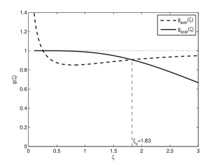
In order to visualize the difference between the low-temperature and scaled low-temperature regimes we may introduce according to (90), (97) and (100) the following two universal functions

$\displaystyle g_{extr}(\zeta)=\frac{\displaystyle f_{magn}^{extr}(T,h)}{\displaystyle f_{magn}(T,h)}=\frac{\displaystyle\sqrt{2\pi}{\rm e}^{\zeta}}{\displaystyle\sqrt{\zeta}\int_{-\pi}^{\pi}{\rm e}^{\zeta\cos{k}}dk},$
gs​c​a​l​(ΞΆ)=fm​a​g​ns​c​a​l​(T,h)fm​a​g​n​(T,h)=π​(4+ΞΆ2)2β€‹βˆ«βˆ’Ο€Ο€e΢​cos⁑k​𝑑k.subscriptπ‘”π‘ π‘π‘Žπ‘™πœsuperscriptsubscriptπ‘“π‘šπ‘Žπ‘”π‘›π‘ π‘π‘Žπ‘™π‘‡β„Žsubscriptπ‘“π‘šπ‘Žπ‘”π‘›π‘‡β„Žπœ‹4superscript𝜁22superscriptsubscriptπœ‹πœ‹superscripteπœπ‘˜differential-dπ‘˜\displaystyle g_{scal}(\zeta)=\frac{\displaystyle f_{magn}^{scal}(T,h)}{f_{magn}(T,h)}=\frac{\displaystyle\pi(4+\zeta^{2})}{\displaystyle 2\int_{-\pi}^{\pi}{\rm e}^{\zeta\cos{k}}dk}. (108)

where $\zeta=\beta|J|$. According to (96), (99) and (108) the extreme low-temperature regime corresponds to $\zeta\gg 1$ and $g_{extr}(\zeta)\approx 1$, while the scaled low-temperature regime corresponds to $\zeta\ll 1$ and gs​c​a​l​(ΞΆ)β‰ˆ1subscriptπ‘”π‘ π‘π‘Žπ‘™πœ1g_{scal}(\zeta)\approx 1. Namely, as it readily follows from (108)

limΞΆβ†’βˆžge​x​t​r​(ΞΆ)=limΞΆβ†’0gs​c​a​l​(ΞΆ)=1.subscriptβ†’πœsubscript𝑔𝑒π‘₯π‘‘π‘Ÿπœsubscriptβ†’πœ0subscriptπ‘”π‘ π‘π‘Žπ‘™πœ1\lim_{\zeta\rightarrow\infty}g_{extr}(\zeta)=\lim_{\zeta\rightarrow 0}g_{scal}(\zeta)=1. (109)

The plots of $g_{extr}(\zeta)$ and gs​c​a​l​(ΞΆ)subscriptπ‘”π‘ π‘π‘Žπ‘™πœg_{scal}(\zeta) are presented in Figure 1.

Refer to caption
Figure 1: Plots of $g_{extr}(\zeta)$ and gs​c​a​l​(ΞΆ)subscriptπ‘”π‘ π‘π‘Žπ‘™πœg_{scal}(\zeta).

From Fig.1 we see that $f^{extr}_{magn}(T,h)$ gives a better approximation to $f_{magn}(T,h)$ than fm​a​g​ns​c​a​l​(T,h)subscriptsuperscriptπ‘“π‘ π‘π‘Žπ‘™π‘šπ‘Žπ‘”π‘›π‘‡β„Žf^{scal}_{magn}(T,h) only for $\zeta>\zeta_{c}\approx 1.83$.

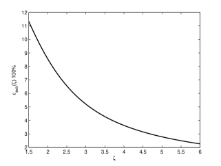
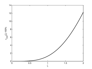
In order to give a more detailed characterization of these approximations we suggest two relative errors functions

Ξ΅a​(ΞΆ)=|fm​a​g​na​(T,h)βˆ’fm​a​g​n​(T,h)fm​a​g​n​(T,h)|=|ga​(ΞΆ)βˆ’1|,a=e​x​t​r,s​c​a​l.formulae-sequencesubscriptπœ€π‘Žπœsuperscriptsubscriptπ‘“π‘šπ‘Žπ‘”π‘›π‘Žπ‘‡β„Žsubscriptπ‘“π‘šπ‘Žπ‘”π‘›π‘‡β„Žsubscriptπ‘“π‘šπ‘Žπ‘”π‘›π‘‡β„Žsubscriptπ‘”π‘Žπœ1π‘Žπ‘’π‘₯π‘‘π‘Ÿπ‘ π‘π‘Žπ‘™\varepsilon_{a}(\zeta)=\left|\frac{f_{magn}^{a}(T,h)-f_{magn}(T,h)}{f_{magn}(T,h)}\right|=|g_{a}(\zeta)-1|,\qquad a=extr,\,scal. (110)

Plots of these functions are presented in Figure 2 and Figure 3.

Refer to caption
Figure 2: Plot of $\varepsilon_{extr}(\zeta)\cdot 100\%$.
Refer to caption
Figure 3: Plot of Ξ΅s​c​a​l​(ΞΆ)β‹…100%β‹…subscriptπœ€π‘ π‘π‘Žπ‘™πœpercent100\varepsilon_{scal}(\zeta)\cdot 100\%.

7 Summary

In the present paper extending the result of [10] belonging to the Ising chain we studied within the QTM approach a highly anisotropic Heisenberg-Ising chain and have suggested the perturbative formula (see (71)-(73)) for the free energy density. At high temperatures the result agrees with the direct high-temperature expansion. At low temperatures an agreement with the cluster expansion is only in the special scaled regime (14) which may be realized only under the condition (98) and for which quantum fluctuations are small against the thermodynamical ones. We suggest that the obtained result confirms effectiveness of the QTM approach and may be extended on perturbative evaluation of correlation functions.

References

  • [1] H. J. Mikeska, A. K. Kolezhuk One-dimensional magnetism Lect. Notes in Phys. 645 1-83 (2004)
  • [2] R. Baxter, Exactly Solved Models in Statistical Mechanics (Academic Press London, 1982)
  • [3] K. Kopinga, M. Steiner, W. J. M. Jonge, Quasi-one-dimensional magnetic behavior of the Ising system ${\rm CsFeCl}_{3}\cdot{\rm 2aq}$, J. Phys. C: Solid State Phys. 18, 3511-3520 (1985)
  • [4] R. E. Greeney, C. P. Landee, J. H. Zhang, W. M. Reiff, One-dimensional Ising ferromagnet $[({\rm CH}_{3})_{2}{\rm NH]FeCl}_{3}\cdot 2{\rm H}_{2}{\rm O}$: Magnetic properties, crystal structure, and ${\rm M\ddot{o}ssbauer}$ spectroscopy, Phys. Rev. B39, 12200-12214 (1989)
  • [5] R. J. C. Dixey, G. B. G. Stenning, P. Manuel, F. Orlandi, P. J. Saines, Ferromagneic Ising chains in frustrated ${\rm LnODCO}_{3}$: the influence of magnetic structure in magnetocaloric frameworks, J. Mater. Chem. C7, 13111 (2019)
  • [6] S. E. Nagler, W. J. L. Buyers, R. L. Armstrong, B. Briat, Ising-like spin-$\frac{1}{2}$ quasi-one-dimensional antiferromagnets: Spin-wave response in ${\rm CsCoX}_{3}$ salts, Phys. Rev. B27, 1784-1799
  • [7] S. Kimura, T. Takeuchi, K. Okunishi, M. Hagiwara, Z. He, K. Kindo, T. Taniyama, M. Itoh, Novel ordering of an S=1/2 quasi one-dimensional Ising-like antiferromagnet in magnetic field, Phys. Rev. Lett. 100, 057202 (2008)
  • [8] A. ${\rm Kl\ddot{u}mper}$, Integrability of quantum chains: theory and applications to the spin-1/2 XXZ chain, in Lect. Notes Phys. 645 (Springer Verlag, Berlin 2004)
  • [9] F. ${\rm G\ddot{o}hmann}$, Statistical mechanics of integrable quantum spin systems, SciPost Phys. Lect. Notes 16 (2020)
  • [10] M. Bortz, F. ${\rm G\ddot{o}hmann}$, Exact thermodynamic limit of short-range correlation functions of the antiferromagnetic XXZ-chain at finite temperatures, Eur. Phys. J. B46, 399 (2005)
  • [11] F. ${\rm G\ddot{o}hmann}$, S. Goomanee, K. K. Kozlowski, J. Suzuki, Thermodynamics of the spin-1/2 Heisenberg-Ising chain at high temperatures: a rigorous approach, Comm. Math. Phys. 377, 627-673 (2020)
  • [12] P. N. Bibikov, Second cluster integral from the spectrum of an infinite $XXZ$ chain, Annals of Phys. 354, 705-714 (2015)