Beyond Discriminant Patterns: On the Robustness of Decision Rule Ensembles

Abstract

Local decision rules are commonly understood to be more explainable, due to the local nature of the patterns involved. With numerical optimization methods such as gradient boosting, ensembles of local decision rules can gain good predictive performance on data involving global structure. Meanwhile, machine learning models are being increasingly used to solve problems in high-stake domains including healthcare and finance. Here, there is an emerging consensus regarding the need for practitioners to understand whether and how those models could perform robustly in the deployment environments, in the presence of distributional shifts. Past research on local decision rules has focused mainly on maximizing discriminant patterns, without due consideration of robustness against distributional shifts. In order to fill this gap, we propose a new method to learn and ensemble local decision rules, that are robust both in the training and deployment environments. Specifically, we propose to leverage causal knowledge by regarding the distributional shifts in subpopulations and deployment environments as the results of interventions on the underlying system. We propose two regularization terms based on causal knowledge to search for optimal and stable rules. Experiments on both synthetic and benchmark datasets show that our method is effective and robust against distributional shifts in multiple environments.

Introduction

Local decision rule learning aims to discover the most discriminant patterns that can distinguish data points with different labels (Hand 2002; Morik and Boulicaut 2005). Local rules are commonly understood to be more explainable and transparent (Fürnkranz, Gamberger, and Lavrač 2012). For example, in clinical health care, one can find rule like “BMI $>$ 25 and Blood pressure $>$ 140 $\rightarrow$ Diagnostic Results”. Domain experts can easily identify useful information to assist decision making (Powers 2020).

Existing work is mainly focused on the discovery of either the most discriminant patterns (Belfodil, Belfodil, and Kaytoue 2018) or fast and high-accuracy ensembles (Chen and Guestrin 2016; Ke et al. 2017). Some recent research started to analyze the fairness of discovered subgroups (Kalofolias, Boley, and Vreeken 2017; Du et al. 2020), the causal rules that are reliable across different subgroups (Budhathoki, Boley, and Vreeken 2021), and rules that can explain the prediction of a groups of neurons (Fischer, Olah, and Vreeken 2021). Some close work employs small amount of data from Randomized Controlled Trials to learn causal invariant random forests (Zeng et al. 2021), or verifies the robustness of tree ensembles with perturbation of samples (Devos, Meert, and Davis 2021). The robustness of decision rule prediction on purely pooled data without knowing the environment label is still underexplored. It is urgent and necessary to investigate whether and how the local decision rules and their ensembles could perform robustly in deployment environments against the distributional shifts (Quiñonero-Candela et al. 2009; Kull and Flach 2014).

In this paper, we consider the problem of distributional shifts from a causal view, as the consequence of interventions on the underlying data generating systems. The goal is to learn a stable classifier that performs robustly across different environments. Existing work either focuses on mitigating the worst case performance of the model on potential environments (Duchi and Namkoong 2021; Sinha et al. 2017; Sagawa et al. 2019), which is called distributional robust optimization (DRO); or focuses on learning causal invariant correlations that can be stable across different environments (Magliacane et al. 2017; Gong et al. 2016; Rojas-Carulla et al. 2018). Solving the invariant learning problem without knowing any additional information is nearly impossible. Existing work requires to know environment labels or causal knowledge represented by Bayesian networks. In this paper, we study this problem by assuming that the environment label is unknown, and the causal graph is partly known. Our aim is to leverage graph criteria that can guide the rule generating algorithms to construct highly predictive and robust decision rules. Specifically, we focus on binary classification in this paper, though it is possible to generalize to multi-class classification.

Main Contributions

• We formulate the problem of robust local decision rule ensembles across various environments. To learn robust decision rules, we propose two regularization terms to encourage the use of causal invariant features for rule generating.

• We propose a graph-based regularization derived from a causal graph and develop a soft mask feature selection method guiding the rule search algorithm.

• We propose a variance-based regularization by introducing artificial features and develop an iterative procedure to guide the rule generating algorithm.

• Experimental results on both synthetic and benchmark datasets demonstrate the effectiveness of our method quantitatively and qualitatively, showing that the two regularization terms are effective in encouraging the algorithms to use invariant features resulting higher robustness across different environments.

Problem Setup

Assume a set of measurable features $X=\{X_{1},\cdots,X_{s}\}$ and label $Y$. Their joint $P(X,Y)$ is governed by an underlying system, where other unmeasurable variables $A$ exist. Following (Arjovsky et al. 2019; Rojas-Carulla et al. 2018), we assume that the datasets $\mathcal{D}=\{D_{e}\}_{1}^{K}$ are collected from a mixture of original environment and environments after interventions. Here $e\in\varepsilon$, $\varepsilon$ denote the environment space. For each environment $e$, $D_{e}=\{x^{i},y^{i}\}_{1}^{N^{e}}$. The robustness of a classifier $F$ will be measured as:

$$\phi(F)=\max_{e\in\varepsilon}\mathbb{E}_{X,Y}[L(Y,F(X))|e].$$

Here, $L:Y\times\hat{Y}\rightarrow\mathbb{R}$ denotes a loss function that measures the performance of a model regarding $Y$, $\hat{Y}$, where $\hat{Y}$ is a random variable representing model predictions. This implies that the robustness of a model $F$ is represented by the worst case performance of $F$ on the potential environments.

We further assume that the values of $X$ are taken from unrestricted domain $\mathcal{A}$. A local decision rule can be defined as a function $r:\mathcal{A}\rightarrow\{-1,1\}$. A data point is covered by rule $r$ as positive sample if and only if $r(x^{i}_{1},\cdots,x^{i}_{s})=1$. The quality of a decision rule is measured by a real-valued function: $\varphi(r)\rightarrow\mathbb{R}$ on how it can discriminate the label $Y$. In this paper, we mainly consider $Y$ as binary class, though it can be generalized to multi-class. Now we formulate the main target problem for this paper:

Problem 1 (Robust Decision Rule Ensembles)

Given a dataset $\mathcal{D}=\{D_{e}\}_{1}^{K}$, $D_{e}=\{x^{i},y^{i}\}_{1}^{N^{e}}$ that comes from an environment governed by a underlying system and other environments after interventions. Without knowing labels of the environments, the task is to learn a classifier $F:\mathcal{X}\rightarrow\mathcal{Y}$ of decision rule ensembles, which can obtain highly predictive performance on the deployment environment that consists of any combination of the potential environments.

The general way to solve this problem is to ensure the performance of the model on each potential environment by applying a measurement. However, since we cannot observe the environment label for the data at hand, we need additional assumptions about the prior knowledge or the structural relations as help. Following (Bühlmann 2020; Gong et al. 2016), we define the following assumptions:

Assumption 1 (Invariant mechanism)

For a set of measurable features $X$ and target label $Y$ under a system with some unmeasurable variables $A$ which might affect both $X$ and $Y$, we assume that it is possible to decompose a subset $X^{\prime}$ from $X$ so that:

$$\forall e\in\varepsilon,P(Y|X^{\prime},e)=P(Y|X^{\prime}).$$

Here we abuse $e$ to represent the potential interventions on the systems because we do not know where the interventions will be added.

Assumption 2 (Sufficient mechanism)

$$\exists f,P(\hat{Y}|X^{\prime})=f(X^{\prime})+P(\epsilon),$$

so that $\mathcal{L}(P(Y|X^{\prime}),P(\hat{Y}|X^{\prime}))<\delta$ holds.

Assumption 1 ensures that it is possible to find a stable mechanism across different interventional environments. Assumption 2 indicates that it is possible to learn a stable mapping function that is sufficient to predict the label $Y$ accurately using the invariant mechanisms.

Now we can formulate the robust decision rule ensembles as an optimization problem:

$$\begin{split}\min_{\{\alpha_{1},\ldots,\alpha_{M}\},\{r_{1},\ldots,r_{M}\}}\max_{e\in\varepsilon}\mathbb{E}_{X,Y}&\left[L\left(Y,\sum_{m=1}^{M}\alpha_{m}\cdot r_{m}(X)\right)\middle|e\right]\\ &+||\alpha||_{2},\end{split}$$ (1)

where

$$r_{m}=\text{arg}\max_{r}\varphi(r).$$ (2)

The objective implies to find a set of rules and their associated coefficients that can minimize the maximal loss across all the environments. By introducing Assumption 1, it is encouraged to construct rules with invariant features, so that the rules can have similar predictive performance across environments. By introducing Assumption 2, rules that are constructed with invariant features are able to achieve highly predictive performance.

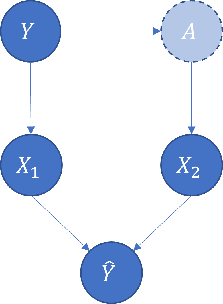
(a) $\mathcal{G}$

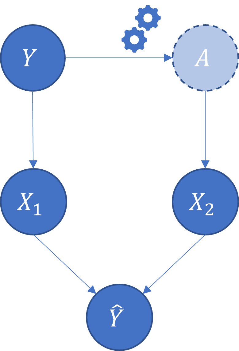
(b) $\mathcal{G}^{\prime}$

Figure 1: Causal graphs representing the data generating process before and after intervention.

Example 1

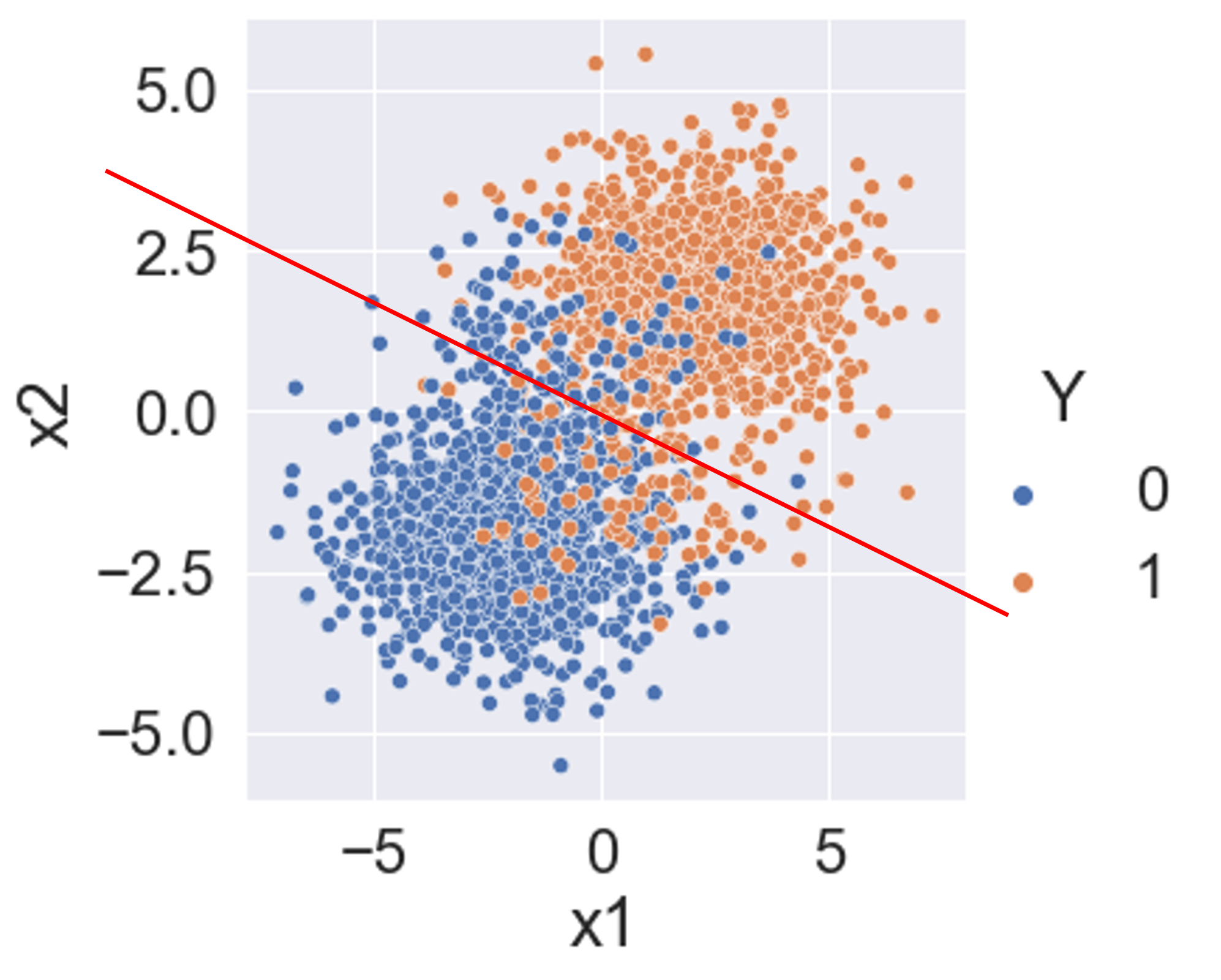
(a) Train data with a non-robust classifier.

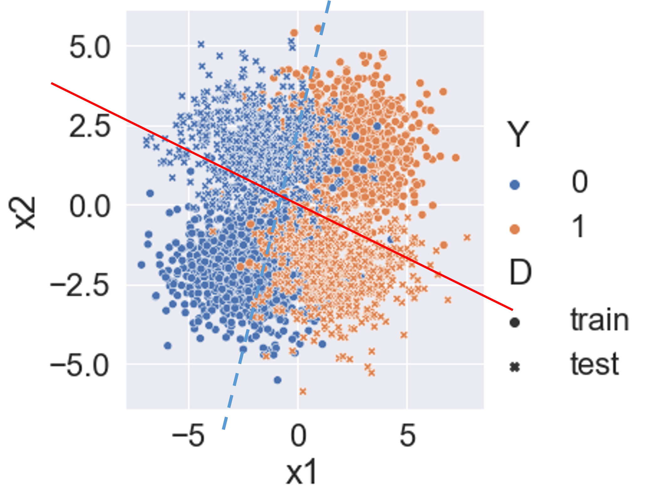
(b) Train and test data with a robust classifier.

Figure 2: Left: a classifier that overfits train data. Right: when adding test data from interventional environments, the previous classifier cannot distinguish target label anymore. A more robust classifier is shown as the dashed line.

We firstly give an example to show how traditional boosting rule ensembles fail on this problem. As shown in Figure 1, the distributional shifts are modeled by a soft intervention (Kocaoglu et al. 2019) on variable $A$, which replaces the original function from $Y$ to $A$. We assume as original data generating process:

$$\begin{array}[]{ll}\phantom{A|}Y\sim\text{Bernoulli}(U_{0}),&X_{1}|Y\sim\mathcal{N}(f_{1}(Y),\sigma_{1}),\\ A|Y\sim\mathcal{N}(f_{2}(Y),\sigma_{2}),&X_{2}|A\sim\mathcal{N}(f_{3}(A),\sigma_{3}),\end{array}$$

where $U_{0},\sigma_{1},\sigma_{2},\sigma_{3}$ are hyper-parameters. According to the local Markov condition (Peters, Janzing, and Schölkopf 2017), the joint distribution $P(X_{1},X_{2},Y,A)$ can be represented as:

$$P(X_{1},X_{2},Y,A)=P(Y)P(X_{1}|Y)P(X_{2}|A)P(A|Y).$$

The intervention implies that $f_{2}(\cdot)$ is replaced with $f_{2}^{\prime}(\cdot)$, so that the joint distribution associated with $G^{\prime}$ (cf. Figure 1b) is shifted by replacing $P(A|Y)$ with $P^{\prime}(A|Y)$. For the learning process, we assume that only $X=\{X_{1},X_{2}\},Y$ are observed; the task is to predict $Y$ with $X$.

We draw 90 percent of train data from joint $P(X,Y)$ and another 10 percent from $P^{\prime}(X,Y)$. For the test data we draw 50 percent from both of them. The data are plotted in Figure 2. The decision rule ensemble algorithm we investigate in this paper is by (Friedman and Popescu 2008). The rule search algorithm is from (Duivesteijn, Feelders, and Knobbe 2016). As shown in Algorithm 1, there are two iterative steps in the learning process: in the boosting step, local rule ensembles are used for loss computation; in the rule generating step, the beam search algorithm evaluates and generates high quality local rules.

Algorithm 1 Local Decision Rule Learning.

1:Dataset $\mathcal{D}$, Quality Measure $\varphi$, Refinement Operator $\eta$, Integer $w$, $d$, $Q$, $M$, $N$,

2:Classifier $F(X)$.

3:function RuleGen($\mathcal{D}$, $\varphi$, $\eta$, $w$, $d$, $Q$, $Res$))

4:     candQ $\leftarrow$ new Queue;

5:     candQ.enqueue($\{\}$);

6:     resultSet $\leftarrow$ new PriorityQueue($Q$);

7:     while level $\leq$ d do

8:         beam $\leftarrow$ new PriorityQueue($w$);

9:         while candQ $\neq$ $\varnothing$ do

10:              seed $\leftarrow$ candQ.dequeue();

11:              set $\leftarrow$ $\eta$(seed);

12:              for all r $\in$ set do

13:                  q $\leftarrow$ $\varphi(r)$;

14:                  resultSet.insert_with_priority(r, q);

15:                  beam.insert_with_priority(r, q);                        

16:         while beam $\neq$ $\varnothing$ do

17:              candQ.enqueue(beam.get_from_element());               

18:     return resultSet;

19:

20:function RuleEnsemble($\mathcal{D}$, $M$, $N$)

21:     $F_{0}(X)=0$;

22:     for $m=1$ to $M$ do

23:         $Res$ $\leftarrow$ $y_{i}-Sigmoid(F(x_{i}))$, $i=1,\cdots,N$;

24:         $r_{m},\alpha_{m}$ $\leftarrow$ RuleGen($\mathcal{D}$, $\varphi$, $\eta$, $w$, $d$, $Q$, $Res$)

25:         $F_{m}(X)\leftarrow F_{m-1}(X)+\alpha_{m}\cdot r_{m}(X)$

26:         $F(X)\leftarrow F_{m}(X)$      

27:     return $F(X)$;

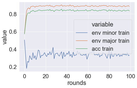
(a) Train.

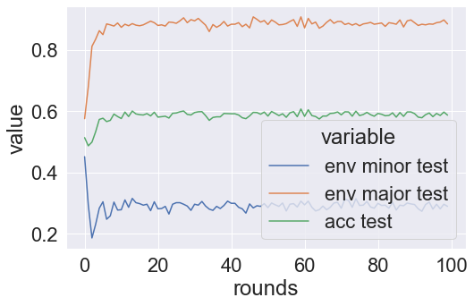
(b) Test.

Figure 3: Accuracy on train and test set, regarding to majority and minority environments.

Table 1: True positive rate of basis decision rules for the ensemble classifier.

$r$	TPR Train	TPR Test
$x7\leq-0.86$ and $x8\phantom{0}>-1.61$	$0.83$	$0.16$
$x9\leq-0.41$ and $x6\phantom{0}\leq-0.88$	$0.85$	$0.18$
$x8>\phantom{-}0.98$ and $x9\phantom{0}>\phantom{-}0.14$	$0.73$	$0.20$
$x8>-0.96$ and $x10>-1.21$	$0.81$	$0.11$
$x6>-0.34$ and $x10\leq-1.21$	$0.79$	$0.13$

As shown in Figure 3, given sufficient boosting iterations, the accuracy on data collected from the majority environment is high. However, the accuracy on data collected from the interventional environment is low. This shows that the patterns in subgroups generated by the interventional environment are ignored; and the model cannot generalize well in the presence of distributional shifts. The same phenomenon is displayed in Table 1, listing 5 rules that are used to build the ensemble classifier. As we can see, the true positive rate of those rules reduce substantially on the test data.

Methodology

The core work of this paper is to investigate the robustness of decision rule ensembles under distributional shifts, and provide a method to ensure the robust performance across various environments. First of all, we need to look into details of the performance of the model.

Robustness Investigation

From Equation (1), we can see that the classifier $F$ is a convex combination of local decision rules. The decision rule generating algorithm plays an important part in our method. In general, we apply a real-valued function $\varphi(\cdot)$ to evaluate each local decision rule. True positive rate and false positive rate are used to evaluate whether a rule can maximally discriminate the target label (Fürnkranz and Flach 2005).

In Algorithm 1, we implemented a quality measure based on that method. Let us recall Example 1; in Table 1, we list some of the rules that are used by the final classifier. As we can see, the true positive rate of those rules deteriorates in the data collected from environment after intervention. This is because the rule generating algorithm selected the variant features that are not against the intervention to construct the rule.

So the question is: in what kind of situation could variant features be naturally selected rather than the invariant feature? The reason might be that the search algorithm is forced to maximize the discriminant patterns, so that the most informative features are selected. We have conducted multiple experiments by investigating the performance of the algorithm regarding to mutual information ratio between invariant and variant features. When the variant features are more informative than the invariant features, the models are very likely to fail on out-of-distribution (OOD) environments. The supplementary material encompasses more details.

Graph-based regularization

From the analysis in the previous section, we know that rule generating algorithm should be aware of the invariant mechanism while searching for the most discriminant features. Feature selection methods are usually known for their effectiveness on improving the generalization ability of the model on OOD data (Chandrashekar and Sahin 2014). In this section, we propose a graph-based method to regularize the feature selection process in the rule generating algorithm.

The core idea is that we can decompose the joint distribution into product conditional distributions of each c-component (Correa and Bareinboim 2019; Tian and Pearl 2002; Pearl 2009). Each variable in c-component is only dependent on its non-descendant variables in the c-component and the effective parents of its non-descendant variables in the c-component. We derive the following theorem for causal invariant decomposition:

Theorem 1

Let $X,Y\subseteq V$ be disjoint sets of variables. Let $W=An(X\cup Y)_{\mathcal{G}}$ be partitioned into c-components $C(W)=\{C_{1}(W_{1}),\ldots,C_{H}(W_{H})\}$ in causal graph $\mathcal{G}_{[An(X\cup Y)]}$. Let $A$ be a set of manipulable variables for potential interventions. Then $X^{\prime}\in C_{h}(W_{h})$ is an invariant feature across interventional environments when either of the following conditions holds:

$$C_{h}(W_{h})\cap A=\emptyset,$$ (3)

$$C_{h}(W_{h})\cap De(Y)=\emptyset,$$ (4)

where $De(Y)$ represents the descendants of $Y$.

We do not specify the direction between feature set $X$ and $Y$. This means that, if there is no direct intervention on $Y$, then features that are parents of $Y$ can be identified as invariant features. Another implication is that if there is an intervention on the Markov blanket of $Y$ that blocks the path from $Y$ to the feature, then we should consider the feature as variant feature.

Given a causal graph by domain knowledge, we can separate invariant subset of features $X^{\prime}$ from $X$. Then the general method is to build a mask set $\{\beta_{1},\ldots,\beta_{s}\}$ where $\beta\in\{0,1\}$ for the feature selection. The optimization problem in Equation (1) can be reformed as:

$$\begin{split}\min_{\{\alpha_{1},\ldots,\alpha_{M}\},\{r_{1},\ldots,r_{M}\}}\max_{e\in\varepsilon}&\mathbb{E}_{X,Y}\left[L\left(Y,\sum_{m=1}^{M}\alpha_{m}\cdot r_{m}(X)\right)\middle|e\right]\\ &+||\alpha||_{2}+||\beta||_{0}.\end{split}$$ (5)

In the rule construction process, we construct the candidate rule by enumerating features one by one. By applying feature masks, the variant features are filtered in this step. Finally, the high quality features are kept for the next beam search iteration. Such a hard selection method might cause high variance and information loss (Maddison, Mnih, and Teh 2016). Following (Yamada et al. 2020), we adapt the soft feature selection method for rule generating algorithm, using Gaussian-based continuous relaxation for Bernoulli variables $\beta$. Here, $\beta_{s}$ is defined by $\beta_{s}=\max(0,\min(1,\mu_{s}+\sigma_{s}))$, where $\sigma_{s}\sim\mathcal{N}(0,\sigma^{2})$. For $X_{s}\in X^{\prime}$, we set $\beta_{s}=0$. For $X_{s}\in X\setminus X^{\prime}$, we set $\mu_{s}$ empirically, according to the mutual information ratio between $I(X_{s};Y)$ and $I(X_{inv};Y)$, where $X_{inv}$ represents $X\setminus X^{\prime}$. Then we sample a $\mu_{s}$ to compute $\beta_{s}$.

In rule generating algorithm we apply Laplace or M-estimate (Cestnik 1990) to measure the quality of discriminant patterns. We define the following quality measure:

$$\varphi(r)=\frac{p+1}{p+n+2}-\lambda\cdot\beta_{s},$$ (6)

where $p$, $n$ denote the positive and negative samples that are covered by the rule, $\lambda$ is scale parameter. By replacing $\varphi(r)$ in Algorithm 1 with Equation (6), we encourage the algorithm to use rules that can maximize the discriminant patterns as well as considering the variant penalties.

Here we recall Example 1 to explain the search process based on Equation (6): in the search process, we equally bin (Meeng and Knobbe 2021) the feature values. Suppose, e.g., we got base rule $r=$ ‘$x_{2}>0$ and $x_{2}<1$’, then we compute the quality of this rule using Equation (6). The highest quality rules are kept in the beam for the next level of search. In the next iteration, we enumerate all the features again. Because the use of the regularization term, in Example 1, the quality of rules including $X_{2}$ are penalized, so that the algorithm are keen to construct rules with $X_{1}$. Then the top rule returned by the beam search algorithm is passed to ‘RuleEnsemble()’ in each boosting step.

Variance-based regularization

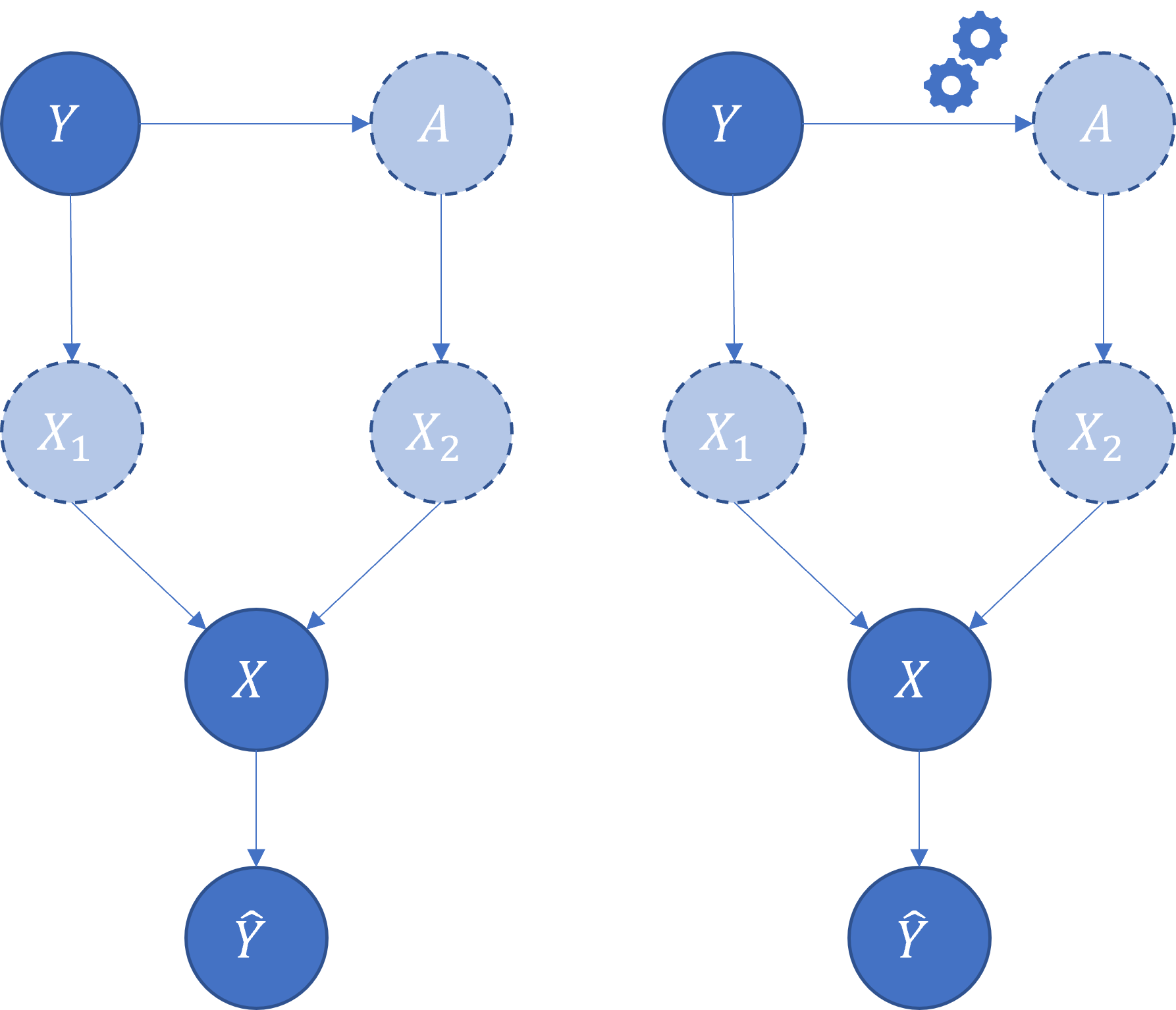
Figure 4: Example 2, causal graph with unobserved features.

In realistic scenarios, it is usually difficult to obtain accurate causal graphs. In some situations, we cannot observe the features that contribute to the mixed features. Here we show Example 2, in which $X_{1}$ and $X_{2}$ are unobservable, while $X$ is derived from the combination of $X_{1},X_{2}$, as shown in Figure 4. It is impossible to decompose invariant features from $X$ directly from the graph. As a consequence, we cannot build masks for feature selection. This usually happens on image datasets. Invariant features include the structures of the objects and variant features include color, background, or lightness.

Previous research (Janzing 2019; Oberst et al. 2021) points out that, by applying regularization properly, a general regressor can gain the causal invariant property. Following this route, we aim to set up a variance-based regularization to build a classifier that uses causal invariant mechanisms. Specifically, we would like to artificially construct a new feature, which is stable with regard to environments and target labels. In Example 2, we can assume that the new feature is the child of $Y$ and parents of $X_{1},X_{2}$. This feature can be used as a proxy to regularize the learning algorithm to employ the causal invariant features for prediction. The variance-based regularization term is adapted according to (Heinze-Deml and Meinshausen 2017):

$$C_{F,\nu}=E[\text{Var}(F(X)|Y,ID)^{\nu}],$$

$$C_{L,\nu}=E[\text{Var}(L(Y,F(X))|Y,ID)^{\nu}],$$

then the optimization problem can be reformed as:

$$\begin{split}\min_{\{\alpha_{1},\ldots,\alpha_{M}\},\{r_{1},\ldots,r_{M}\}}\max_{e\in\varepsilon}&\mathbb{E}_{X,Y}\left[L\left(Y,\sum_{m=1}^{M}\alpha_{m}\cdot r_{m}(X)\right)\middle|e\right]\\ &+||\alpha||_{2}+C,\end{split}$$ (7)

where $C$ is a general representation of $C_{F,\nu}$, $C_{L,\nu}$. Here the challenges are twofold. On the one hand, as opposed to neural networks (where the regularization term is used to guide the optimization of weights), in our case, the regularization should be used for the rule generating algorithm. On the other hand, the variance is computed on global data, while the traditional rule search algorithm only considers local discriminant patterns. How to enclose the variance to guide the search of local rule, which further benefits the ensembles, is a challenge.

Specifically, we can compute $C_{L,1}$ as:

$$\hat{C}_{L,1}=\frac{1}{q}\sum_{j=1}^{q}\frac{1}{|G_{j}|}\sum_{i\in G_{j}}(L(Y,F(x_{i}))-\hat{\mu}_{L,j})^{2},$$

where

$$\hat{\mu}_{L,j}=\frac{1}{|G_{j}|}\sum_{i\in G_{j}}L(Y,F(x_{i})).$$

We employ the exponential loss function:

$$L(Y,F(X))=e^{-Y\cdot F(X)},$$

where for each new candidate rule in step $m$, we have:

$$e^{-Y\cdot F_{m}(X)}=e^{-Y\cdot(F_{m-1}(X)+\alpha_{m}r_{m}(X))}.$$ (8)

By this definition, we can iteratively compute the variance term in each boosting loop for each candidate rule. Then the quality measure can be reformulated as:

$$\varphi(r)=\frac{p+1}{p+n+2}-\lambda\cdot C_{L,F_{m-1},r_{m},\nu}.$$ (9)

This enables the search algorithm to select local decision rules with highly discriminant patterns as well as low global variance in each boosting step. Rather then only considering TPR and FPR, with Equation (9), we can compute the influence of the new added rule to the global level by computing the variance. Equation (8) allows us to reuse the results in previous boosting steps, reducing the computional cost. The same method can be applied to compute $C_{F,\nu}$.

Experiments

In this section, we design multiple experiments to validate our method against the following questions:

RQ1 How effectively can graph-based regularization ensure the robustness of decision rule ensembles?

RQ2 How effectively can variance-based regularization ensure the robustness of decision rule ensembles?

Implementation

We mainly consider beam search parameter: width $w$, depth $d$ and regularization scale $\lambda$; the boosting rounds $M$; and the environmental parameter: number of environments $K$. We fix the beam search width to $30$, depth to $3$ and boosting rounds to $100$. Experiments are varied by different regularization scale $\lambda$ and number of environments $K$. For all the experiments, we collect training data from one majority environment and several minority environments. For test data, we use data from several potential environments. We run the experiments on multiple synthetic and benchmark datasets. All the experiments are conducted on a single CPU (i5-11600K) desktop.

Experiments on graph-based regularization

To validate RQ1, we design experiments on synthetic data based on Example 1, and a public benchmark.

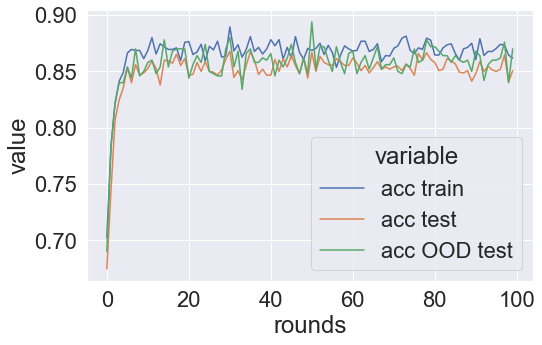
Figure 5: Accuracy on train, test, OOD test for synthetic data in Example 1 with graph-based regularization.

Table 2: Example 1, TPR and FPR of basis decision rules for the ensemble classifier.

$r$	TPR, FPR	TPR, FPR
	Train	Test
$x8>1.01$ and $x3>-1.90$	$0.56$, $0.08$	$0.50$, $0.18$
or $x2>3.06$
$x3>-2.23$ and $x4>-1.88$	$0.80$, $0.15$	$0.71$, $0.22$
and $x5>-3.57$
$x1>-2.69$ and $x2>0.71$	$0.71$, $0.14$	$0.69$, $0.23$
or $x1>3.96$
$x9>-0.66$ and $x3>0.31$	$0.70$, $0.19$	$0.59$, $0.26$
or $x1>2.22$
$x4>1.30$ or $x5>2.72$	$0.80$, $0.19$	$0.68$, $0.21$
or $x2>5.59$

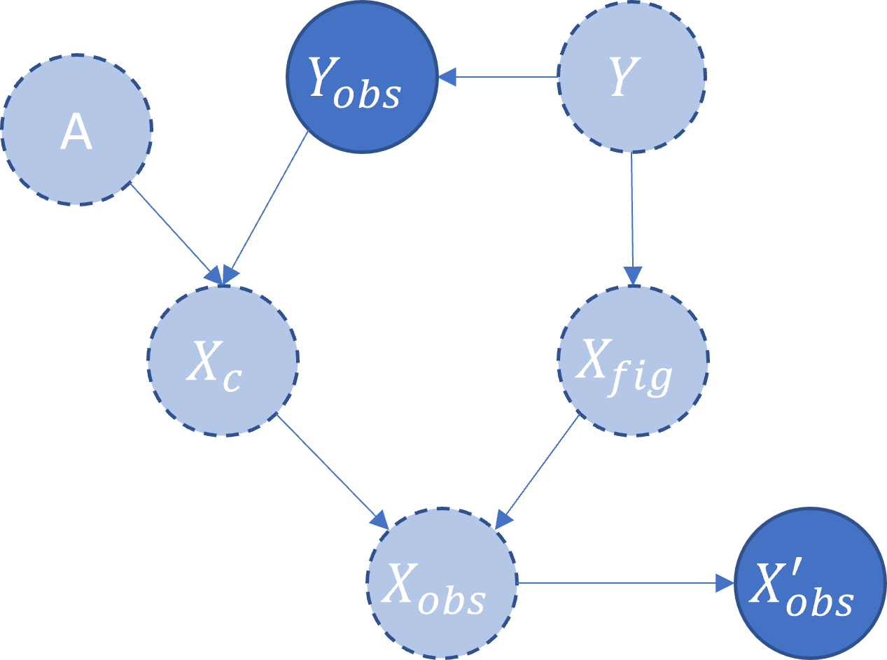
Figure 6: Generating process for CMNIST benchmark.

The public benchmark that we use is introduced by (Aubin et al. 2021). The problem is a linear version of spiral binary classification called ‘small invariant margin’ (Parascandolo et al. 2020). We would like to test the performance of our method on multiple environments. Hence, we first sample a set of $K$ environments $\{e\}^{K}$. Then, according to the data generating process $P(X,Y|e)$, we sample data for each of the environments $\{D_{e}\}_{1}^{K}$, $D_{e}=\{X^{i},Y^{i}\}^{n_{e}}_{1}$. Similar as Example 1, in each generating loop, we sample invariant feature set $X_{inv}$ and variant feature set $X_{var}$ then concatenate them to construct the observable features. Data sampled from various environments are scrambled by a full rank matrix. By this setting, the pooled data prevents us from using a small subset to construct the invariant predictor.

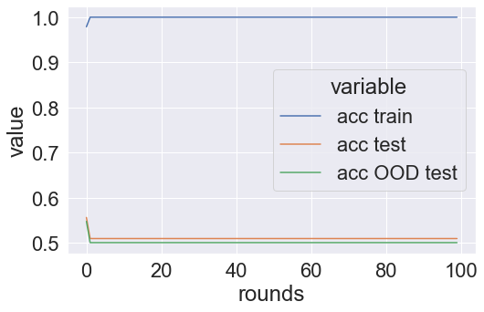
(a) before regularization.

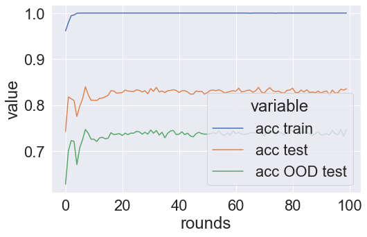
(b) graph-based regularization.

Figure 7: Accuracy on train, test, OOD test for benchmark dataset with 3 environments.

Table 3: Public benchmark (‘small invariant margin’), TPR and FPR of basis decision rules for the ensemble classifier.

$r$	TPR, FPR	TPR, FPR
	Train	Test
$x6>0.55$ or $x5\leq-0.09$	$0.97$, $0.003$	$0.55$, $0.32$
and $x6>-0.88$
$x6>-0.88$ and $x2\leq-0.15$	$0.98$, $0.02$	$0.68$, $0.27$
and $x4\leq 0.10$
$x2\leq-0.13$ or $x6>0.55$	$0.98$, $0.06$	$0.63$, $0.31$
or $x1\leq-0.07$
$x3\leq 0.02$ and $x4\leq-0.01$	$0.98$, $0.03$	$0.65$, $0.33$
or $x6>0.55$
$x1<0.04$ and $x6>0.88$	$0.91$, $0.01$	$0.63$, $0.33$
and $x5\leq 0.08$

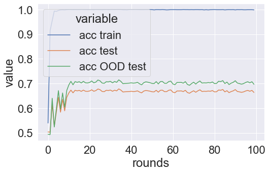
(a) env5

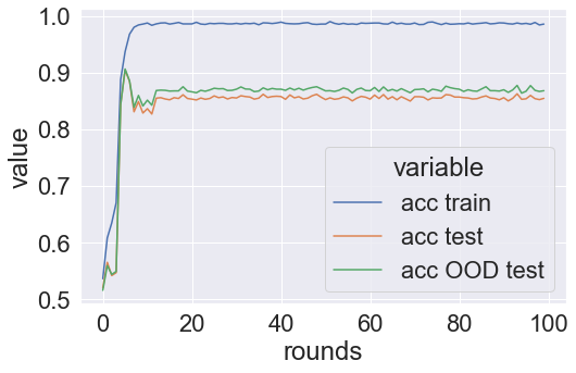
(b) env7

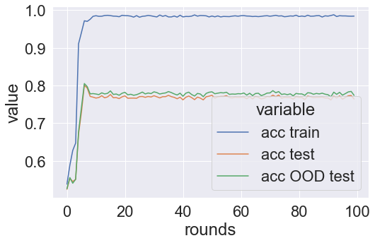
(c) env10

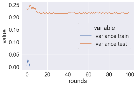
(d) env5

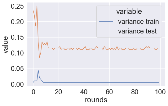
(e) env7

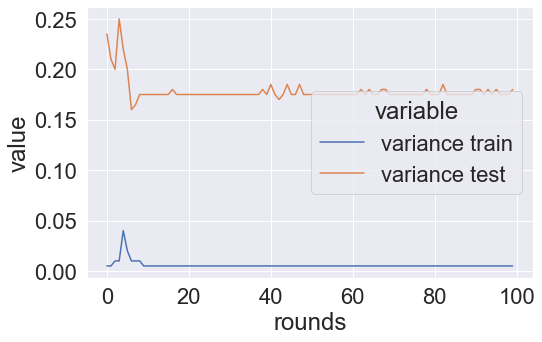
(f) env10

Figure 8: Performance on ‘small invariant margin’ benchmark. We show that variance-based regularization is effective to improve the robustness.

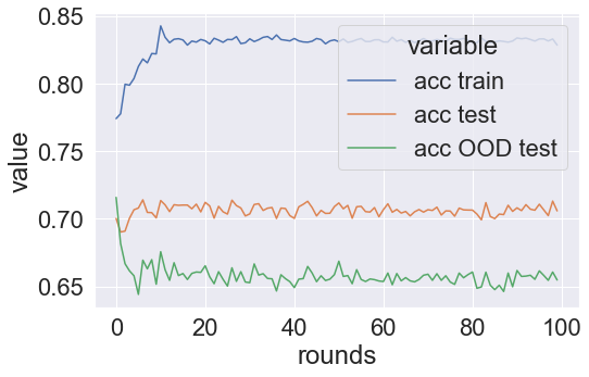
(a) $\lambda=1$.

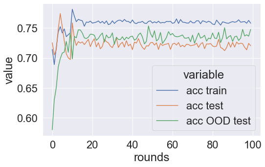
(b) $\lambda=3$.

Figure 9: Accuracy on train, test, OOD test for color MNIST benchmark with different $\lambda$ settings.

Figure 5 shows the results with graph-based regularization for Example 1. As we can see, compared with Figure 3, the accuracy on test and OOD test data are significantly improved. This shows that the decomposition of invariant features from causal graph is sufficient to estimate the target label. In Table 2, we list basis rules that are used for the classifier. Here, $x_{1},\ldots,x_{5}$ are invariant features, and $x_{6},\ldots,x_{9}$ are variant features. As we can see, the TPR and FPR are relatively worse in test environments but still keep good prediction performance. Also because of the using of soft mask for feature selection process, some variant features also contribute to the construction of basis rules. This shows that the soft mask feature selection can regularize the algorithm for high discriminant patterns as well as keeping stable across different environments.

In Figure 7, we plot the results on benchmark ‘small invariant margin’. With a naive setting of the rule ensemble classifier, the accuracy on training data can reach $1.0$. However, the test and OOD test accuracy are close to a random guess. This means that the model is fully governed by the variant features. In Figure 7b, the results show that after graph regularization, the test and OOD test accuracy are substantially improved. In Table 3, we list several basis rules. As we can see, the basis rules are highly discriminant on training environments, while the TPR and FPR are worse in test environments but still have good prediction performance. Some variants also contribute to the construction of rules. These results show that soft mask for feature selection based on graph regularization is effective against distributional shift.

Experiments on variance-based regularization

To validate RQ2, we design experiments on one benchmark (‘small invariant margin’) dataset also used in the previous section, and another benchmark called color MNIST (Arjovsky et al. 2019). For the former benchmark, we construct the artificial feature ‘ID’ according to two groups of invariant features in the original generating process. We test the performance of our method by varying the the number of potential environments $5,7,10$ with dimension of invariant and variant features setting to $5,5$. As shown in Figure 8, the variance-based regularization is effective in improving the robustness of the model across multiple environments, without knowing the environment labels. We also notice that the test accuracies on minority data are even a bit better. This shows that with the restricting of the regularization term, the rule search algorithm sacrifices the accuracy to explore invariant patterns.

In this paper, we adapt the generating process of color MNIST (Koyama and Yamaguchi 2020). In order to reduce the rule search space, the final dimension of input features is reduced to $50$ by applying SVD transform. This can still keep the structural property for predictive information. We calculate the variance by constructing additional features regarding to each digit number as same group. As shown in Figure 12, we plot the performance of our method with regularization scale setting to $1,3$. This shows that, with lower scale, the algorithm is encouraged to use more discriminant patterns. With larger regularization scale, the variance term restricts the use of variant features, which improves the robustness of the model.

Finally, in order to compare our method with baselines, we run boosting classifier implemented in sklearn (Pedregosa et al. 2011) on those benchmarks (cf. Table 4).

Table 4: Performance of Traditional Boosting classifier on benchmarks.

Dataset	Traditional Boosting
Example 1	$0.5235$
CMNIST	$0.5004$
‘small invariant margin’ 13	0.5160
‘small invariant margin’ 15	0.5432
‘small invariant margin’ 17	0.3009
‘small invariant margin’ 10	0.5318

Conclusion

In this paper, we study the problem of robustness of local decision rule ensembles. Local decision rules could provide both high predictive performance and explainability. However, the stability of those explanations given by the rules is still underexplored. Our work aims to fill this gap. We start from analyzing the robustness of decision rule ensembles guided by potential causal graph. Empirical results show how the performance of traditional rule ensembles vary across environments. The distributional shifts are assumed to be caused by potential interventions on the underlying system. We further propose two regularization terms to improve the robustness of decision rule ensembles. The graph-based term is built by decomposing invariant features using a given causal graph; the variance-based term relies on an additional artificial feature that can restrict the model’s decision boundary within groups. We conduct experiments on several synthetic and benchmark datasets. The experimental results show that our method can significantly improve the robustness of rule ensembles across environments.

Appendix A Robustness investigation

We apply a mutual information measure between features and the target label. Then according to the ratio of mutual information score between variant and invariant features, we run the model on different realizations of Example 1. The results are shown in Figure 10. As we can see, the performance of the model on OOD test environment are highly correlated with the ratio. This means that when the variant features are more informative than the invariant features in the given datasets, the models are very likely to fail on OOD environments.

In order to mitigate this risk, we propose to apply regulation on the rule generating algorithm forcing it to learn the rules using causal invariant features.

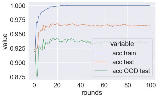
(a) 1

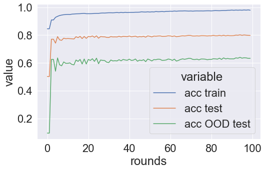
(b) 3

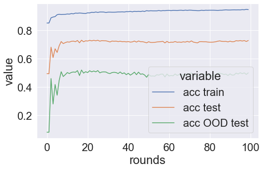
(c) 5

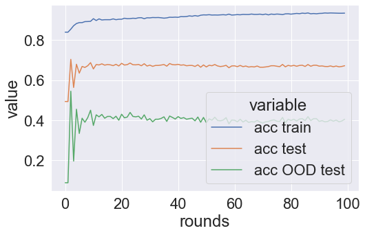
(d) 7

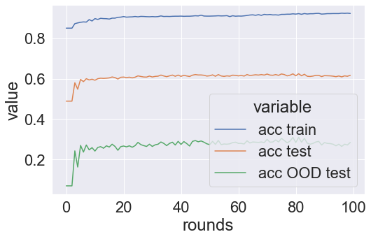
(e) 10

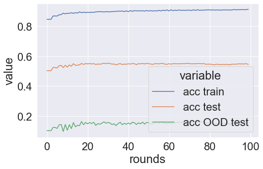
(f) 15

Figure 10: Comparison for the performance of decision rule ensemble regarding to the mutual information ratio between variant and invariant features.

Appendix B Invariant feature decomposition

The core idea is that we can decompose the joint distribution into product conditional distributions of each c-component (Correa and Bareinboim 2019; Tian and Pearl 2002; Pearl 2009). Each variable in c-component is only dependent on its non-descendant variables in the c-component and the effective parents of its non-descendant variables in the c-component. We derive the following theorem for causal invariant decomposition:

Theorem 2

Let $X,Y\subseteq V$ be disjoint sets of variables. Let $W=An(X\cup Y)_{\mathcal{G}}$ be partitioned into c-components $C(W)=\{C_{1}(W_{1}),\ldots,C_{H}(W_{H})\}$ in causal graph $\mathcal{G}_{[An(X\cup Y)]}$. Let $A$ be a set of manipulable variables for potential interventions. Then $X^{\prime}\in C_{h}(W_{h})$ is an invariant feature across interventional environments when either of the following conditions holds:

$$C_{h}(W_{h})\cap A=\emptyset,$$ (10)

$$C_{h}(W_{h})\cap De(Y)=\emptyset,$$ (11)

where $De(Y)$ represents the descendants of $Y$.

Proof 1

First, from Assumption 1 we can know $A\cap Pa(Y)=\emptyset$. When $C_{h}(W_{h})\cap A=\emptyset$, there is no manipulable variable in $C_{h}(W_{h}$. Because each variable in c-component is only dependent on its non-descendant variables in the c-component and the effective parents of its non-descendant variables in the c-component, we have $P(Y|X_{h},A)=P(Y|X_{h})$. When $C_{h}(W_{h})\cap De(Y)=\emptyset$, $X_{h}$ can block the path from $A_{h}$ to $Y$, then we have $P(Y|X_{h},A_{h})=P(Y|X_{h})$.

Algorithm 2 Invariant feature decomposition.

1:Dataset $\Omega$, Graph $\mathcal{G}$, c-components decomposition operator $\psi$

2:$X^{\prime}$

3:function CCS($\Omega,\mathcal{G}$, $\psi$)

4:     $X^{\prime}\leftarrow\{\}$;

5:     $W\leftarrow An(X\cup Y)_{\mathcal{G}}$;

6:     $C_{1}(W_{1}),\cdots,C_{H}(W_{H})\leftarrow\psi(G_{[An(X\cup Y)]})$;

7:     for $h=1$ to $H$ do

8:         if $C_{h}(W_{h})\cap A=\emptyset$ then

9:              $X^{\prime}\leftarrow C_{h}(W_{h})$;          

10:         if $C_{h}(W_{h})\cap De(Y)=\emptyset$ then

11:              $X^{\prime}\leftarrow C_{h}(W_{h})\setminus A$               

12:     return $X^{\prime}$;

We developed Algorithm 2 to find set of invariant features $X^{\prime}$. The c-component decomposition operator $\psi$ is based on (Tian and Pearl 2002).

Appendix C Details of rule ensemble learning

Problem 2 (Robust Decision Rule Ensembles)

Given a dataset $\mathcal{D}=\{D_{e}\}_{1}^{K}$, $D_{e}=\{x^{i},y^{i}\}_{1}^{N^{e}}$ that comes from an environment governed by a underlying system and other environments after interventions. Without knowing labels of the environments, the task is to learn a classifier $F:\mathcal{X}\rightarrow\mathcal{Y}$ of decision rule ensembles, which can obtain highly predictive performance on the deployment environment that consists of any combination of the potential environments.

Here we recall Algorithm 1 to explain how do we plan to solve Problem 2 by learning the invariant and sufficient mapping function. As shown in Figure 11, there are mainly two iterative steps in decision rule ensemble learning: in the rule generating step, the algorithm enumerate features and their combination to seek a rule that can maximally discriminate the target label, a subset of features and values ranges are considered to construct the decision rule; in the boosting step, the model are evaluated based on all the learned rules, and the residuals calculated are propagated to the rule generating algorithm for next iteration. Here in Figure 11, we abuse $l,r$ to represent the cutting point in feature’s value space. $l$ represents the left cutting point, $r$ represents the right cutting point.

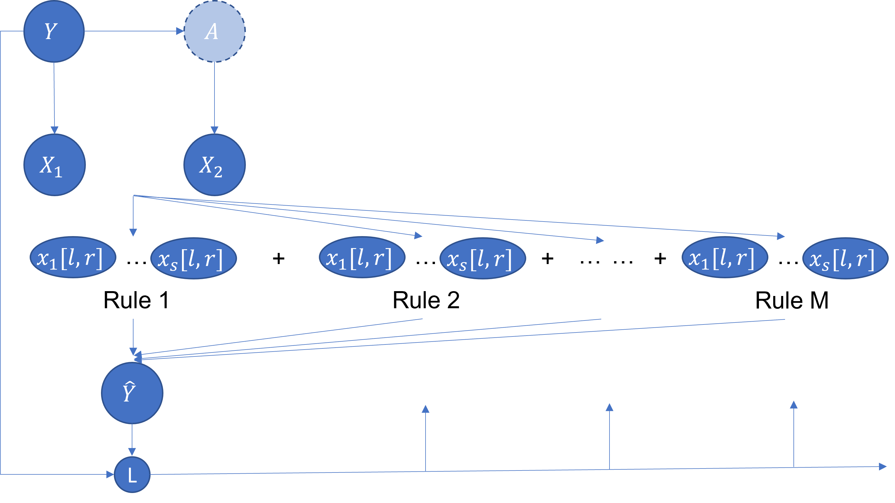
Figure 11: Decision Rule Ensemble Learning.

Appendix D Variance-based regularization

For each single decision rule, we have $r(x)\in\{-1,1\}$. Hence we have $F(x)=\sum_{m=1}^{M}\alpha_{m}r_{m}(x)\in\mathbb{R}$. Then we can map the output to $[0,1]$ by applying the sigmoid funciton. Here we abuse $F(x)$ as $Sigmoid(F(x))$. Here we recall:

$$C_{F,\nu}=E[\text{Var}(F(X)|Y,ID)^{\nu}],$$

specifically, following (Heinze-Deml and Meinshausen 2017), we can compute $C_{F,1}$ as:

$$\hat{C}_{F,1}=\frac{1}{q}\sum_{j=1}^{q}\frac{1}{|G_{j}|}\sum_{i\in G_{j}}(F(x_{i})-\hat{\mu}_{F,j})^{2},$$

where

$$\hat{\mu}_{F,j}=\frac{1}{|G_{j}|}\sum_{i\in G_{j}}F(x_{i}).$$

This variance term indicates that the decision boundary of $F(x)$ for data points in same group by artificial feature and label should be similar, quantifying by the predictive probability.

Appendix E Details of Datasets

‘small invariant margin’

This benchmark is from (Aubin et al. 2021), as a linear version of spiral binary classification problem which is originally introduced by (Parascandolo et al. 2020). The basic idea is to create variant features with large-margin decision boundary and invariant features with small-margin decision boundary. For each specific environment $e\in\varepsilon$, the data generating process is:

$$\begin{split}&y\sim\text{Bernoulli}(U_{0}),\\ &\text{when}\quad y=0,\\ &x_{inv}\sim\mathcal{N}(\gamma,10^{-1}),\quad x_{spu}\sim\mathcal{N}(\mu,10^{-1}),\\ &\text{when}\quad y=1,\\ &x_{inv}\sim\mathcal{N}(-\gamma,10^{-1}),\quad x_{spu}\sim\mathcal{N}(-\mu,10^{-1}),\end{split}$$

where $\mu\sim\mathcal{N}(0,1)$, $\gamma=0.1\cdot 1_{d_{inv}}$. For different, we sample different $\mu$, so that the patterns in variant features vary across environments. The input features can be scrambled by a fixed random rotation matrix across potential environments. This prevents the algorithms from using a small subset to make invariant prediction. We generate datasets both with and without scrambles.

‘cows versus camels’

This benchmark is also from (Aubin et al. 2021), as an imitation version of binary classification problem for cows and camels. The variant feature is denoted by the background (Beery, Van Horn, and Perona 2018). The intuition is ‘most cows appear in grass and most camels appear in sand’. For this benchmark, our method always achieves accuracy $1.0$, TPR $1.0$ and FPR $0.0$, which is similar with (Koyama and Yamaguchi 2020). So we think it is meaningless to discuss the performance on this benchmark.

For benchmarks ‘cows versus camels’ and ‘small invariant margin’, we sample the datasets using open source from Github https://github.com/facebookresearch/InvarianceUnitTests.

Color MNIST

For this benchmark, we following the original version from (Arjovsky et al. 2019). The data generating process is:

$$\begin{split}&\text{If digit}(Y)<5:Y_{obs}=0,\\ &\text{else}:Y_{obs}=1,\\ &t\sim\mathcal{U}(0,1),\\ &\text{If}\quad t<0.25:Y_{obs}=-Y_{obs},\\ &X_{fig}\sim f_{1}(Y)+\sigma,\\ &\text{color C}(X_{c})=f_{2}(Y_{obs})+f_{3}(A),\\ &X_{obs}=X_{fig}\times[X_{c},(1-X_{c}),0],\\ &X_{obs}^{\prime}=\text{SVD}(X_{obs}),\end{split}$$

where SVD represents Singular value decomposition (Wall, Rechtsteiner, and Rocha 2003). In Figure 12, we plot some data samples of generated images. In Figure 13, we visualize the final input data with t-SNE (Van der Maaten and Hinton 2008). As we can see, the patterns for each digits are kept in the transformed feature space. The reason is to reduce the dimension of feature space for the rule constructing. Even though with the increase of search depth in beam search, it is possible to explore the rules in original space.

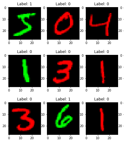
Figure 12: Samples in Color MNIST.

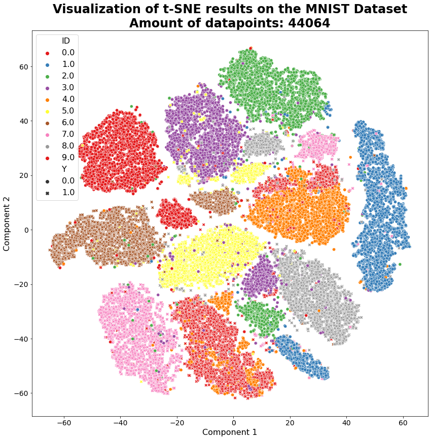
Figure 13: t-SNE visualization of final observations for Color MNIST.

References

- Arjovsky et al. (2019) Arjovsky, M.; Bottou, L.; Gulrajani, I.; and Lopez-Paz, D. 2019. Invariant risk minimization. arXiv preprint arXiv:1907.02893.
- Aubin et al. (2021) Aubin, B.; Słowik, A.; Arjovsky, M.; Bottou, L.; and Lopez-Paz, D. 2021. Linear unit-tests for invariance discovery. arXiv preprint arXiv:2102.10867.
- Beery, Van Horn, and Perona (2018) Beery, S.; Van Horn, G.; and Perona, P. 2018. Recognition in terra incognita. In Proceedings of the European conference on computer vision (ECCV), 456–473.
- Belfodil, Belfodil, and Kaytoue (2018) Belfodil, A.; Belfodil, A.; and Kaytoue, M. 2018. Anytime subgroup discovery in numerical domains with guarantees. In Joint European Conference on Machine Learning and Knowledge Discovery in Databases, 500–516. Springer.
- Budhathoki, Boley, and Vreeken (2021) Budhathoki, K.; Boley, M.; and Vreeken, J. 2021. Discovering reliable causal rules. In Proceedings of the 2021 SIAM International Conference on Data Mining (SDM), 1–9. SIAM.
- Bühlmann (2020) Bühlmann, P. 2020. Invariance, causality and robustness. Statistical Science, 35(3): 404–426.
- Cestnik (1990) Cestnik, B. 1990. Estimating probabilities: A crucial task in machine learning. In Proc. 9th European Conference on Artificial Intelligence, 1990.
- Chandrashekar and Sahin (2014) Chandrashekar, G.; and Sahin, F. 2014. A survey on feature selection methods. Computers & Electrical Engineering, 40(1): 16–28.
- Chen and Guestrin (2016) Chen, T.; and Guestrin, C. 2016. Xgboost: A scalable tree boosting system. In Proceedings of the 22nd acm sigkdd international conference on knowledge discovery and data mining, 785–794.
- Correa and Bareinboim (2019) Correa, J. D.; and Bareinboim, E. 2019. From statistical transportability to estimating the effect of stochastic interventions. In Proceedings of the Twenty-Eighth IJCAI-19.
- Devos, Meert, and Davis (2021) Devos, L.; Meert, W.; and Davis, J. 2021. Versatile Verification of Tree Ensembles. In International Conference on Machine Learning, 2654–2664. PMLR.
- Du et al. (2020) Du, X.; Pei, Y.; Duivesteijn, W.; and Pechenizkiy, M. 2020. Fairness in network representation by latent structural heterogeneity in observational data. In 34th AAAI conference on Artificial Intelligence (AAAI2020).
- Duchi and Namkoong (2021) Duchi, J. C.; and Namkoong, H. 2021. Learning models with uniform performance via distributionally robust optimization. The Annals of Statistics, 49(3): 1378–1406.
- Duivesteijn, Feelders, and Knobbe (2016) Duivesteijn, W.; Feelders, A. J.; and Knobbe, A. 2016. Exceptional model mining. Data Mining and Knowledge Discovery, 30(1): 47–98.
- Fischer, Olah, and Vreeken (2021) Fischer, J.; Olah, A.; and Vreeken, J. 2021. What’s in the Box? Exploring the Inner Life of Neural Networks with Robust Rules. In International Conference on Machine Learning, 3352–3362. PMLR.
- Friedman and Popescu (2008) Friedman, J. H.; and Popescu, B. E. 2008. Predictive learning via rule ensembles. The Annals of Applied Statistics, 2(3): 916–954.
- Fürnkranz and Flach (2005) Fürnkranz, J.; and Flach, P. A. 2005. Roc ‘n’rule learning—towards a better understanding of covering algorithms. Machine learning, 58(1): 39–77.
- Fürnkranz, Gamberger, and Lavrač (2012) Fürnkranz, J.; Gamberger, D.; and Lavrač, N. 2012. Foundations of rule learning. Springer Science & Business Media.
- Gong et al. (2016) Gong, M.; Zhang, K.; Liu, T.; Tao, D.; Glymour, C.; and Schölkopf, B. 2016. Domain adaptation with conditional transferable components. In International conference on machine learning, 2839–2848. PMLR.
- Hand (2002) Hand, D. J. 2002. Pattern detection and discovery. In Pattern Detection and Discovery, 1–12. Springer.
- Heinze-Deml and Meinshausen (2017) Heinze-Deml, C.; and Meinshausen, N. 2017. Conditional variance penalties and domain shift robustness. arXiv preprint arXiv:1710.11469.
- Janzing (2019) Janzing, D. 2019. Causal regularization. arXiv preprint arXiv:1906.12179.
- Kalofolias, Boley, and Vreeken (2017) Kalofolias, J.; Boley, M.; and Vreeken, J. 2017. Efficiently discovering locally exceptional yet globally representative subgroups. In 2017 IEEE International Conference on Data Mining (ICDM), 197–206. IEEE.
- Ke et al. (2017) Ke, G.; Meng, Q.; Finley, T.; Wang, T.; Chen, W.; Ma, W.; Ye, Q.; and Liu, T.-Y. 2017. Lightgbm: A highly efficient gradient boosting decision tree. Advances in neural information processing systems, 30: 3146–3154.
- Kocaoglu et al. (2019) Kocaoglu, M.; Jaber, A.; Shanmugam, K.; and Bareinboim, E. 2019. Characterization and learning of causal graphs with latent variables from soft interventions. In Advances in Neural Information Processing Systems, 14369–14379.
- Koyama and Yamaguchi (2020) Koyama, M.; and Yamaguchi, S. 2020. Out-of-distribution generalization with maximal invariant predictor. arXiv preprint arXiv:2008.01883.
- Kull and Flach (2014) Kull, M.; and Flach, P. 2014. Patterns of dataset shift. In First International Workshop on Learning over Multiple Contexts (LMCE) at ECML-PKDD.
- Maddison, Mnih, and Teh (2016) Maddison, C. J.; Mnih, A.; and Teh, Y. W. 2016. The concrete distribution: A continuous relaxation of discrete random variables. arXiv preprint arXiv:1611.00712.
- Magliacane et al. (2017) Magliacane, S.; van Ommen, T.; Claassen, T.; Bongers, S.; Versteeg, P.; and Mooij, J. M. 2017. Domain adaptation by using causal inference to predict invariant conditional distributions. arXiv preprint arXiv:1707.06422.
- Meeng and Knobbe (2021) Meeng, M.; and Knobbe, A. J. 2021. For real: a thorough look at numeric attributes in subgroup discovery. Data Mining and Knowledge Discovery, 35(1): 158–212.
- Morik and Boulicaut (2005) Morik, K.; and Boulicaut, J.-F. 2005. Local Pattern Detection: International Seminar Dagstuhl Castle, Germany, April 12-16, 2004, Revised Selected Papers, volume 3539. Springer Science & Business Media.
- Oberst et al. (2021) Oberst, M.; Thams, N.; Peters, J.; and Sontag, D. 2021. Regularizing towards Causal Invariance: Linear Models with Proxies. arXiv preprint arXiv:2103.02477.
- Parascandolo et al. (2020) Parascandolo, G.; Neitz, A.; Orvieto, A.; Gresele, L.; and Schölkopf, B. 2020. Learning explanations that are hard to vary. arXiv preprint arXiv:2009.00329.
- Pearl (2009) Pearl, J. 2009. Causality. Cambridge university press.
- Pedregosa et al. (2011) Pedregosa, F.; Varoquaux, G.; Gramfort, A.; Michel, V.; Thirion, B.; Grisel, O.; Blondel, M.; Prettenhofer, P.; Weiss, R.; Dubourg, V.; Vanderplas, J.; Passos, A.; Cournapeau, D.; Brucher, M.; Perrot, M.; and Duchesnay, E. 2011. Scikit-learn: Machine Learning in Python. Journal of Machine Learning Research, 12: 2825–2830.
- Peters, Janzing, and Schölkopf (2017) Peters, J.; Janzing, D.; and Schölkopf, B. 2017. Elements of causal inference: foundations and learning algorithms.
- Powers (2020) Powers, D. M. 2020. Evaluation: from precision, recall and F-measure to ROC, informedness, markedness and correlation. arXiv preprint arXiv:2010.16061.
- Quiñonero-Candela et al. (2009) Quiñonero-Candela, J.; Sugiyama, M.; Lawrence, N. D.; and Schwaighofer, A. 2009. Dataset shift in machine learning. Mit Press.
- Rojas-Carulla et al. (2018) Rojas-Carulla, M.; Schölkopf, B.; Turner, R.; and Peters, J. 2018. Invariant models for causal transfer learning. The Journal of Machine Learning Research, 19(1): 1309–1342.
- Sagawa et al. (2019) Sagawa, S.; Koh, P. W.; Hashimoto, T. B.; and Liang, P. 2019. Distributionally robust neural networks for group shifts: On the importance of regularization for worst-case generalization. arXiv preprint arXiv:1911.08731.
- Sinha et al. (2017) Sinha, A.; Namkoong, H.; Volpi, R.; and Duchi, J. 2017. Certifying some distributional robustness with principled adversarial training. arXiv preprint arXiv:1710.10571.
- Tian and Pearl (2002) Tian, J.; and Pearl, J. 2002. On the testable implications of causal models with hidden variables. In Proceedings of the Eighteenth conference on Uncertainty in artificial intelligence, 519–527. Morgan Kaufmann Publishers Inc.
- Van der Maaten and Hinton (2008) Van der Maaten, L.; and Hinton, G. 2008. Visualizing data using t-SNE. Journal of machine learning research, 9(11).
- Wall, Rechtsteiner, and Rocha (2003) Wall, M. E.; Rechtsteiner, A.; and Rocha, L. M. 2003. Singular value decomposition and principal component analysis. In A practical approach to microarray data analysis, 91–109. Springer.
- Yamada et al. (2020) Yamada, Y.; Lindenbaum, O.; Negahban, S.; and Kluger, Y. 2020. Feature selection using stochastic gates. In International Conference on Machine Learning, 10648–10659. PMLR.
- Zeng et al. (2021) Zeng, S.; Bayir, M. A.; Pfeiffer III, J. J.; Charles, D.; and Kiciman, E. 2021. Causal transfer random forest: Combining logged data and randomized experiments for robust prediction. In Proceedings of the 14th ACM International Conference on Web Search and Data Mining, 211–219.