Improving the Silicon Interactions of GFN-xTB

Abstract

A general-purpose Density Functional Tight Binding method, the GFN-xTB model is gaining increased popularity in accurate simulations that are out of scope for conventional ab initio formalisms. We show that in its original GFN1-xTB parametrization, organosilicon compounds are described poorly. This issue is addressed by re-fitting the model’s silicon parameters to a data set of ten thousand reference compounds, geometry-optimized with the revPBE functional. The resulting GFN1-xTB-Si parametrization shows improved accuracy in the prediction of system energies, nuclear forces and geometries and should be considered for all applications of the GFN-xTB Hamiltonian to systems that contain silicon.

CCM]Center for Molecular Modeling (CMM), Ghent University, Technologiepark-Zwijnaarde 46, B-9052, Ghent, Belgium CCM]Center for Molecular Modeling (CMM), Ghent University, Technologiepark-Zwijnaarde 46, B-9052, Ghent, Belgium

1 Background & Summary

Silicon is the second most abundant element on earth.¹ Its physical properties make it a crucial building block for applications in electronics^{2, 3, 4} and materials science.^{5, 6, 7} More recently organosilicon compounds have become of increasing interest to the field of organic synthesis in the role of (selective) intermediates^{8, 9, 10} or catalysts.^{11, 12} One way scientists can study any of the aforementioned applications is through computational simulations of appropriate systems on modern computer hardware. Compared to experimental laboratory work, this domain of computational chemistry offers a high amount of flexibility when it comes to throughput, man-hours and overall cost. A myriad of models can be employed to simulate a system of interest – too many to give a a comprehensive overview of all of them here (we point the reader to Refs. 13, 14 for a comprehensive introduction to the topic). Instead, we roughly classify two fundamental model types: ab initio and empirical. The former describes a model that is derived from the fundamental laws of physics and, without introducing approximations fitted to (experimental) reference data. Examples of ab initio models are the Hartree-Fock (HF) formalism, configuration interaction (CI) methods and density functional theory (DFT) with non-empirical functionals like PBE ¹⁵. Explicit treatment of the electronic structure means that ab initio computations can be highly accurate, but computationally slow and only limited to small systems of roughly tens to hundreds of atoms. Empirical models in contrast are fast and can handle system sizes of up to millions of atoms. This speed-up is achieved through simplifications in the description of interatomic interactions. Examples for empirical models are classical force fields (FF) or machine learning potentials (MLP). One benefit of empirical models is the ability to fit their parameters to a specific chemical space. This allows for an improvement in prediction accuracy without the need to switch to a computationally more expensive model. The semi-empirical GFN1-xTB¹⁶ formalism falls under this category. The model has found a broad application in the modeling of small-to-medium organic molecules, where it is predominantly used for geometry optimizations ^{17, 18, 19, 20}. Despite its success, we have observed large discrepancies between GFN1-xTB and DFT when comparing relative energies, optimized geometries and nuclear gradients of organosilicon compounds. This issue is addressed by fitting the silicon parameters of GFN1-xTB to higher-level DFT data. We describe a reference data set of 10000 organosilicon compounds, followed by the parameter optimization procedure in the Methods Section. The Results Section discusses shortcomings of the original GFN1-xTB model in more detail and compares it to our newly obtained parameters as well as to similar models from the literature. In contrast to the original parametrization, our parameters reproduce system energies and geometries more accurately, without compromise to the prediction accuracy of non-silicon organic compounds, as tested on a subset of the ANI-1x²¹ data.

2 Methods

Organosilicon Reference Data

Initial structures for our reference data set are taken from the PubChem library.^{22, 23} The search query included the following filters:

• Heavy atom count between 1 and 15

• Compound contains Si, O, C

• Covalent unit count of 1

• Molecular weight less or equal to 200 g/mol

• Total formal charge of 0

From the total of 50750 compounds matching the query, a random subset of 10k structures is selected. The resulting set has a mean heavy atom count of 10.5 (smallest: 3, largest: 13, standard deviation: 1.9). In addition to the chemical elements defined in the search query, H, N, Cl, S, F, P and Br are included in the set. Elemental occurrences are presented in Table LABEL:tab:occurrences, with nitrogen being the most, and bromine the least prominent among the additional elements (other than Si, O and C) in the set. All structures are geometry-optimized with the Amsterdam Density Functional²⁴ (ADF) molecular simulation package, as integrated in the Amsterdam Modeling Suite²⁵. We use the revPBE functional, ^{26, 27} a ’Small’ frozen core and the double-zeta polarized (DZP) basis set. Geometry convergence criteria are left at their default values, namely 0.001 Hartree/Å, 0.00001 Hartree/Atom and 0.1 Å for atomic gradients, energy and atomic displacements respectively. A Quasi-Newton optimizer²⁸ in the delocalized coordinates space is used for the optimizations. Distributions of all the convergence criteria at each structure’s last optimization step are provided in Figure S1. Training and validation data sets are constructed from (1) atomic forces at the initial (un-optimized) geometries, considering Si atoms only, (2) energy differences between the same compound’s initial and optimized geometries, (3) root-mean-square deviation (RMSD) of the optimized geometries. Prior to the construction of the data sets, improbable outlier geometries are filtered by excluding 123 systems with an energy difference larger than 5 kJ/mol per atom between optimized and initial geometries.

Table 1: Elemental occurrences in the reference data set. Structures containing at least one atom of the listed element are counted in the upper part. Structures with the exact number of silicon atoms are counted in the lower part.

Element	Occurrence
C	10000
O	10000
Si	10000
H	9994
N	3252
Cl	573
S	461
F	295
P	85
Br	27
1 Si	9318
2 Si	613
3 Si	59
4 Si	9
5 Si	1

2.1 Optimization of the Silicon GFN-xTB Parameters

Developed by Grimme et al., the GFN-xTB (also GFN1-xTB) model is a semiempirical method for the computation of a chemical system’s Hamiltonian.¹⁶ The method follows a Density Functional Tight Binding (DFTB) approximation, which describes the electronic energy $E_{\mathrm{el}}$ of a molecule as a functional of its (valence) electron density $\rho(\bm{r})=\rho_{0}(\bm{r})+\delta\rho(\bm{r})$, where $\bm{r}$ is a spatial coordinate.^{29, 30} The reference density $\rho_{0}$ is typically a superposition of individual atomic contributions, whereas $\delta\rho$ is the consequence chemical bonding and is assumed to be relatively small. In the DFTB formalism, the energy is approximated by a Taylor series up to the third order in $\delta\rho$ (corresponding to DFTB3), such that

$$E_{\mathrm{el}}[\rho]=E^{0}[\rho_{0}]+E^{1}[\rho_{0},(\delta\rho)^{1}]+E^{2}[\rho_{0},(\delta\rho)^{2}]+E^{3}[\rho_{0},(\delta\rho)^{3}].$$ (1)

The total GFN1-xTB energy is divided into electronic (el), repulsive (rep), dispersion (disp) and halogen-bonding (xb) interactions and can be written as

$$E=E_{\mathrm{el}}+E_{\mathrm{rep}}+E_{\mathrm{disp}}+E_{\mathrm{xb}}.$$ (2)

Reference 16 describes the GFN-xTB Hamiltonian in more detail.

The parameter optimization is performed with the ParAMS parameter fitting package.³¹ Starting from Grimme’s original parametrization¹⁶, we optimize all 17 silicon parameters from the electronic and repulsive terms, plus one parameter specific to the Si-O atom-pair for a total of 18 parameters. A summary of all optimized parameters, and their values in the original parametrization are provided in Table LABEL:tab:params along with upper and lower parameter ranges that were used during the optimization. Training and validation sets are created by randomly splitting the complete data set into relative sizes of 80 and 20 percent respectively (splitting is based on unique structures, not their properties). Within the training set, each entry of relative energies, atomic forces and RMSD is assigned a weight of 2.4, 28.0 and 1.0 respectively. The weights were determined by minimizing the standard deviation of all per-entry contributions to the overall root-mean-square error (RMSE), as calculated with the initial GFN1-xTB parameters. Covariance matrix adaptation evolution strategy (CMA-ES)^{32, 33}, a gradient-free, population-based optimization algorithm is used to optimize the GFN-xTB parameters. Population size and initial sampling width $\sigma$ are set to 12 and 0.2 respectively. The optimization is set up to run for a maximum of 72 hours. To prevent a waste of computation time when stuck in local minima, an early stopping algorithm is set up to abort the optimization if there is no improvement in the training set loss after 1000 evaluations. At every optimization step, only a batch of 800 randomly selected jobs is computed to speed up convergence. To compensate for both, the noise introduced through the aforementioned batching and the pseudo-random sampling of CMA-ES, 8 independent optimizations are performed. The best parameter set is selected based the lowest training set loss function value.

Table 2: List of all optimized parameter names (Si only where applicable, atomic subscript dropped), their initial values and the equation number that lists the parameter as described in Ref. 16, followed by the optimization bounds used in this work and the optimized values.

Parameter	Equation	Original Value	Optimization Bounds	Optimized Value
$\eta$	5	+0.438	(+0.100, +3.500)	+2.251
$\Gamma$	9	+1.500	(+1.000, +2.000)	+1.125
$\alpha$	13	+0.948	(+0.500, +1.800)	+1.036
$Z$	13	+16.898	(+8.000, +25.000)	+21.357
$EN$	10	+1.900	(+1.710, +2.090)	+2.089
$K_{\mathrm{SiO}}$	10	+1.000	(+0.900, +1.100)	+0.969
3s level
$k^{\mathrm{poly}}_{l}$	11	-14.202	(-24.000, +15.000)	+14.825
$\kappa^{l}$	5	+0.000	(-10.000, +10.000)	-4.972
$H^{l}$	12	-14.506	(-30.000, -2.000)	-20.800
$\zeta_{l}$	7	+1.522	(+0.400, +4.000)	+2.337
3p level
$k^{\mathrm{poly}}_{l}$	11	-3.893	(-10.000, +30.000)	-8.629
$\kappa^{l}$	5	-5.926	(-10.926, -0.926)	-6.046
$H^{l}$	12	-7.557	(-17.557, +2.443)	-3.526
$\zeta_{l}$	7	+1.609	(+0.400, +4.000)	+1.576
3d level
$k^{\mathrm{poly}}_{l}$	11	+25.499	(-30.000, +44.000)	+36.572
$\kappa^{l}$	5	+0.000	(-10.000, +10.000)	+6.072
$H^{l}$	12	-2.508	(-12.508, +7.492)	-3.321
$\zeta_{l}$	7	+1.169	(+0.400, +4.000)	+2.474

3 Results and Discussion

Performance of Models from the Literature

To serve as a baseline, the performance of three DFTB parametrizations from the literature is compared on our validation set. The first three rows of Figure 1 compare three general-purpose models, namely GFN1-xTB¹⁶ (the initial parameter set used for our optimizations), GFN2-xTB³⁴ and the QUASINANO2015³⁵ set. Overall, GFN2-xTB (Fig. 1 second row) is the most accurate of the three, with the lowest errors in the energy differences and the RMSD of geometry-optimized structures. Both GFN models predict atomic forces with the same accuracy (Fig. 1 middle column, first and second rows). Although the QUASINANO2015 parameters are the least accurate of the three when comparing relative energies and atomic forces, distributions of the RMSD are better than for GFN1-xTB. We found that in most cases, the poor RMSD of GFN1-xTB can be traced back to unrealistic Si-O-R bond angles. This problem is visualized in Figure 2, showing the distributions of all Si-O-C angles for each of the aforementioned models. Note how DFT predicts an average angle of 121 degrees (Fig. 2a), while most angles computed with GFN1-xTB are almost colinear with an angle close to 180 degrees (Fig. 2b). This issue is not observed for the GFN2-xTB and QUASINANO2015 models (Fig. 2c,d). In more extreme cases geometry optimizations with GFN1-xTB resulted in rearrangements and bond dissociations. One example is presented in Figure 3, showing the optimized structure of sulfosilyloxymethane, as computed with revPBE and GFN1-xTB.

Optimized Silicon Parameters for GFN1-xTB

We report all optimized parameter values in Table LABEL:tab:params. Following the previous section, we compare our new set of parameters, which we refer to as GFN1-xTB-Si, in the last row of Figure 1 and Figure 2e. Substantial improvements can be observed in all three of the fitted properties, bringing GFN1-xTB-Si to an accuracy level that is comparable to GFN2-xTB. At the same time, calculations with the GFN1-xTB Hamiltonian have shown to be roughly 35% faster when compared to the GFN2-xTB model. This has been tested by randomly selecting a batch of 200 geometries from our data set and measuring the time it took both models to calculate energies and atomic forces for all structures. The set-up has been repeated 100 times to produce average timings.

A sanity check is performed by calculating the atomic gradients on a separate test set. We use the ANI-1x reference data by Smith et al.²¹ for this purpose, which includes atomic gradients calculated with the $\omega B97X$³⁶ functional. The test set is constructed from one randomly selected conformation for each of the 3113 unique configurations in the ANI-1x data. Atomic gradients are computed with the GFN1-xTB and GFN1-xTB-Si parameters. As expected, both parametrizations predict the same forces for the test set, since the ANI-1x data does not include any silicon atoms. A correlation plot between the $\omega B97X$ and GFN1-xTB forces is presented in Figure S2. For the ANI-1x set, the RMSE of the atomic gradients is roughly 28.5 kJ/mol/Å. This leads us to the conclusion that the GFN1-xTB-Si parametrization can be used without any compromises when computing energies, gradients and geometries of isolated organic compounds.

We would like to stress that this work introduces a parameter set that has been fitted to geometries, nuclear gradients and energies, and as such should only be used for applications related to these properties. This forms a contrast to the original claim of the GFN model – the ability to represent Geometries, Frequencies and Non-covalent interactions accurately, as the latter two properties have neither been investigated nor fitted here. Although this calls for a future investigation, we argue that a first focus on corrected geometries, forces and energies is most logical since (1) optimized geometries are the most popular prediction target when using GFN1-xTB^{17, 18, 19, 20} and (2) we expect that predictions of frequencies and non-covalent interactions on systems with poorly-described geometries and energies will be of limited interest. Furthermore, the reduced error on the silicon forces for slightly distorted geometries suggests that the Hessian of the potential energy improved as well, which should be beneficial for the prediction of vibrational frequencies.

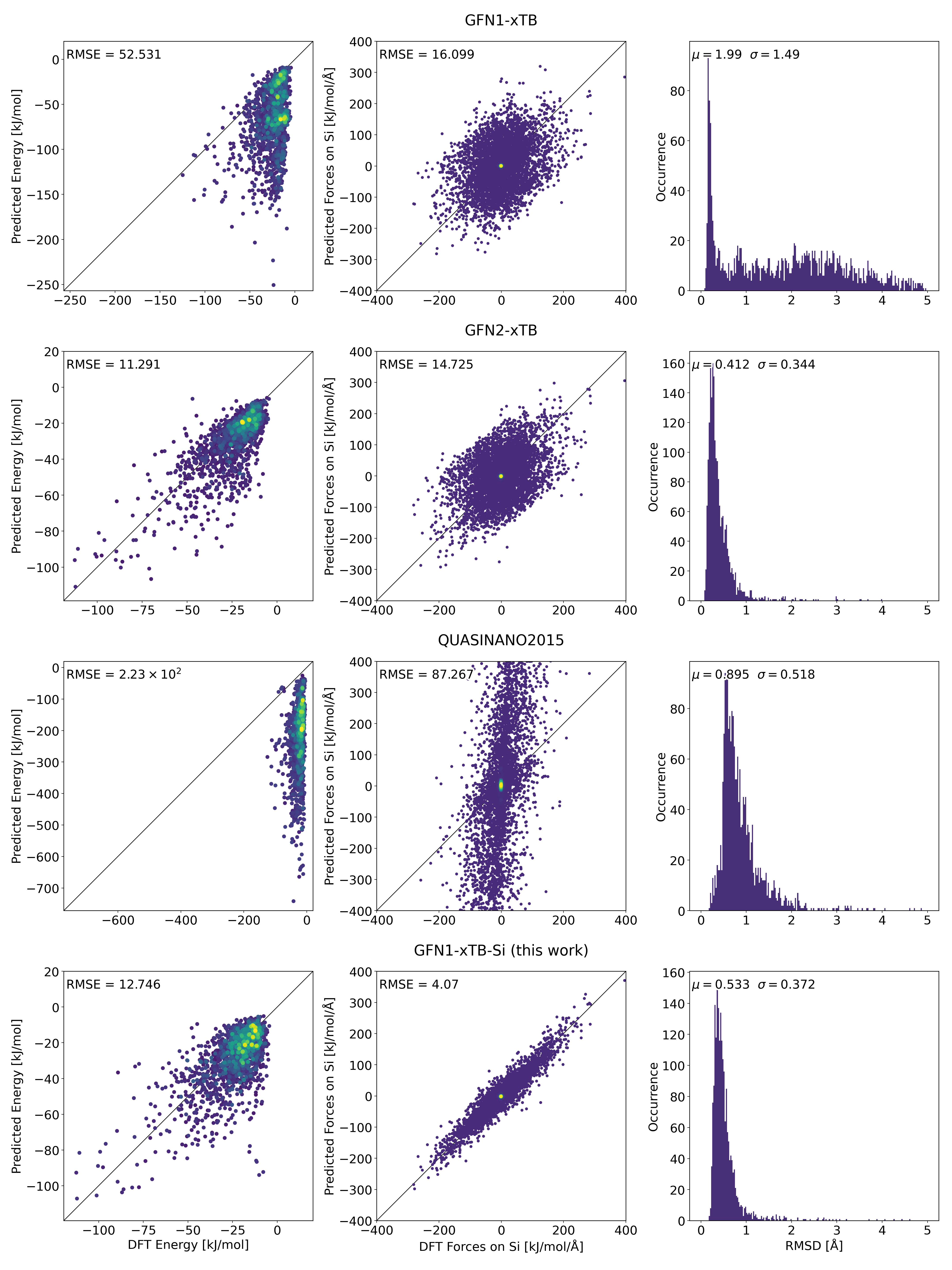
Figure 1: Validation set performance of various Density Functional Tight Binding models. Comparing GFN1-xTB¹⁶, GFN2-xTB³⁴, QUASINANO2015³⁵ and this GFN1-xTB-Si (this work) from top to bottom. Columns, from left to right depict energy differences, force components on the Si atoms, and RMSD of atomic positions (as described in the Methods Section). X and Y values in the first two columns are reference properties and their DFTB predictions respectively. Areas of lower point densities are depicted in dark blue; higher densities in bright green. Root-mean-square error (RMSE) printed in the same units as the axes. Histograms in the right column show the RMSD between geometry-optimized reference and DFTB structures. Mean $\mu$ and standard deviation $\sigma$ printed in ångström.

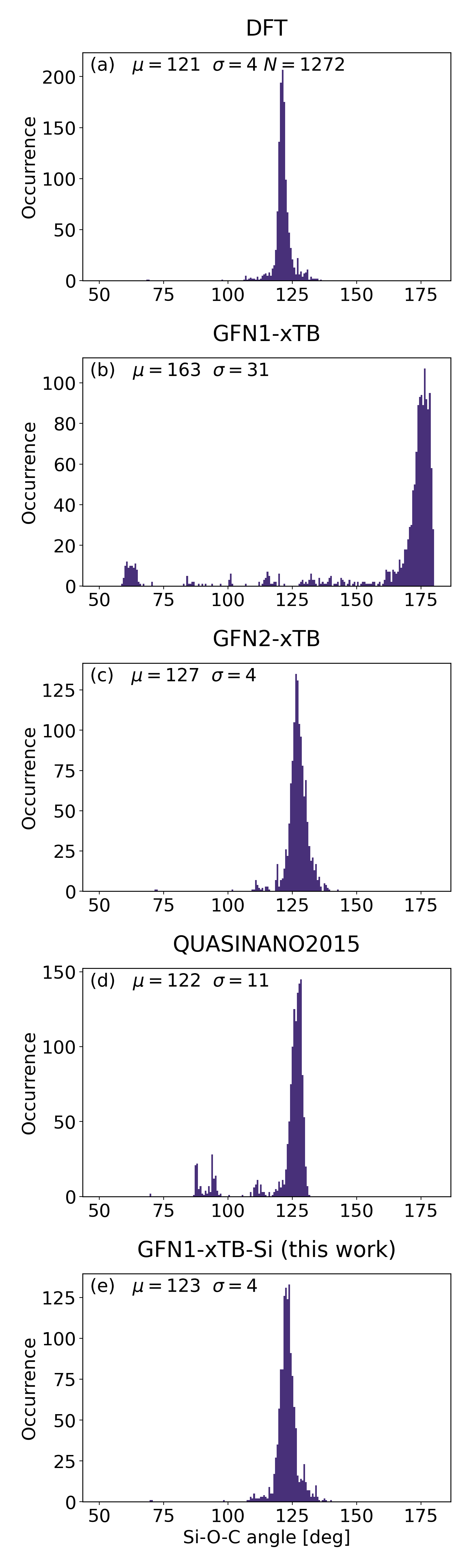
Figure 2: Si-O-C angle distributions of all optimized structures in the validation set. Comparing the revPBE²⁷, GFN1-xTB¹⁶, GFN2-xTB³⁴, QUASINANO2015³⁵ and this GFN1-xTB-Si (this work) in a,b,c,d,e respectively. Printed text shows mean ($\mu$), standard deviation ($\sigma$) and the total number of points ($N$).

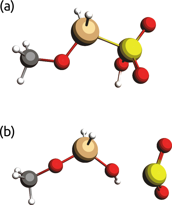
Figure 3: Optimized geometries of sulfosilyloxymethane (PubChem ID 154240983). Structures optimized with (a) revPBE and (b) GFN1-xTB. The latter shows a re-arrangement and Si-O-R angles close to 180 degrees. Hydrogen, carbon, oxygen, silicon and sulfur depicted in white, grey, red, beige and yellow respectively.

4 Data and Software Availability

GFN1-xTB-Si parameters (in the AMS format), reference data, including training and validation sets, and files needed to run the parameter optimization scheme are available at DOI: 10.24435/materialscloud:14-4m or the Materials Cloud Archive record 2021.152. See the Supporting Information or data repository for a description of the reference data formats. For the ANI-1x test set, please refer to Ref. 21. The Amsterdam Modeling Suite²⁵ (v. 2020.203), which includes the ParAMS package³¹ (v. 0.5.1), is a commercial software, for which a free trial may be requested at www.scm.com.

5 Acknowledgements

This project has received funding from the European Union’s Horizon 2020 research and innovation programme under grant agreement No 814143. T.V. acknowledges funding of the research board of Ghent University. The computational resources (Stevin Supercomputer Infrastructure) and services used in this work were provided by the VSC (Flemish Supercomputer Center), funded by Ghent University, FWO and the Flemish Government – department EWI.

Author contributions statement

L.K. designed and performed the study. Both authors wrote the manuscript. T.V. oversaw the project

Competing interests

The authors declare no competing interests.

References

- Rumble 2020 Rumble, J. CRC handbook of chemistry and physics : a ready-reference book of chemical and physical data; CRC Press/Taylor & Francis Group, 2020
- McConnell et al. 1992 McConnell, H. M.; Owicki, J. C.; Parce, J. W.; Miller, D.; Baxter, G. s.; Wada, H. G.; Pitchford, S. The cytosensor microphysiometer: biological applications of silicon technology. Science 1992, 257, 1906–1912
- Bruel 1995 Bruel, M. Silicon on insulator material technology. Electronics letters 1995, 31, 1201–1202
- Chapin et al. 1954 Chapin, D. M.; Fuller, C. S.; Pearson, G. L. A new silicon p-n junction photocell for converting solar radiation into electrical power. Journal of Applied Physics 1954, 25, 676–677
- Baerlocher et al. 2007 Baerlocher, C.; McCusker, L. B.; Olson, D. H. Atlas of zeolite framework types; Elsevier, 2007
- Park et al. 2009 Park, J.-H.; Gu, L.; Von Maltzahn, G.; Ruoslahti, E.; Bhatia, S. N.; Sailor, M. J. Biodegradable luminescent porous silicon nanoparticles for in vivo applications. Nature materials 2009, 8, 331–336
- Yang et al. 2012 Yang, P.; Gai, S.; Lin, J. Functionalized mesoporous silica materials for controlled drug delivery. Chemical Society Reviews 2012, 41, 3679–3698
- Zhang et al. 2013 Zhang, H.-J.; Priebbenow, D. L.; Bolm, C. Acylsilanes: valuable organosilicon reagents in organic synthesis. Chemical Society Reviews 2013, 42, 8540
- Lalonde and Chan 1985 Lalonde, M.; Chan, T. Use of organosilicon reagents as protective groups in organic synthesis. Synthesis 1985, 1985, 817–845
- Hatanaka and Hiyama 1991 Hatanaka, Y.; Hiyama, T. Highly selective cross-coupling reactions of organosilicon compounds mediated by fluoride ion and a palladium catalyst. Synlett 1991, 1991, 845–853
- dos Santos et al. 2000 dos Santos, J. H. Z.; Greco, P. P.; Stedile, F. C.; Dupont, J. Organosilicon-modified silicas as support for zirconocene catalyst. Journal of Molecular Catalysis A: Chemical 2000, 154, 103–113
- Walker et al. 2019 Walker, J. C. L.; Klare, H. F. T.; Oestreich, M. Cationic silicon Lewis acids in catalysis. Nature Reviews Chemistry 2019, 4, 54–62
- Cramer 2004 Cramer, C. Essentials of computational chemistry : theories and models; Wiley: Chichester, West Sussex, England Hoboken, NJ, 2004
- Frenkel 2002 Frenkel, D. Understanding molecular simulation : from algorithms to applications; Academic Press: San Diego, 2002
- Perdew et al. 1996 Perdew, J.; Burke, K.; Ernzerhof, M. Generalized Gradient Approximation Made Simple. Physical review letters 1996, 77, 3865–3868, Number: 18
- Grimme et al. 2017 Grimme, S.; Bannwarth, C.; Shushkov, P. A Robust and Accurate Tight-Binding Quantum Chemical Method for Structures, Vibrational Frequencies, and Noncovalent Interactions of Large Molecular Systems Parametrized for All spd-Block Elements (Z = 1–86). Journal of Chemical Theory and Computation 2017, 13, 1989–2009
- Cavasin et al. 2018 Cavasin, A. T.; Hillisch, A.; Uellendahl, F.; Schneckener, S.; Göller, A. H. Reliable and Performant Identification of Low-Energy Conformers in the Gas Phase and Water. Journal of Chemical Information and Modeling 2018, 58, 1005–1020
- Hahn et al. 2018 Hahn, R.; Bohle, F.; Fang, W.; Walther, A.; Grimme, S.; Esser, B. Raising the Bar in Aromatic Donor–Acceptor Interactions with Cyclic Trinuclear Gold(I) Complexes as Strong -Donors. Journal of the American Chemical Society 2018, 140, 17932–17944
- Casajus et al. 2020 Casajus, H.; Dubreucq, E.; Tranchimand, S.; Perrier, V.; Nugier-Chauvin, C.; Cammas-Marion, S. Lipase-Catalyzed Ring-Opening Polymerization of Benzyl Malolactonate: An Unusual Mechanism? Biomacromolecules 2020, 21, 2874–2883
- Backhouse et al. 2021 Backhouse, O. J.; Santana-Bonilla, A.; Booth, G. H. Scalable and Predictive Spectra of Correlated Molecules with Moment Truncated Iterated Perturbation Theory. The Journal of Physical Chemistry Letters 2021, 12, 7650–7658
- Smith et al. 2020 Smith, J. S.; Zubatyuk, R.; Nebgen, B.; Lubbers, N.; Barros, K.; Roitberg, A. E.; Isayev, O.; Tretiak, S. The ANI-1ccx and ANI-1x data sets, coupled-cluster and density functional theory properties for molecules. Scientific Data 2020, 7
- Kim et al. 2018 Kim, S.; Chen, J.; Cheng, T.; Gindulyte, A.; He, J.; He, S.; Li, Q.; Shoemaker, B. A.; Thiessen, P. A.; Yu, B.; Zaslavsky, L.; Zhang, J.; Bolton, E. E. PubChem 2019 update: improved access to chemical data. Nucleic Acids Research 2018, 47, D1102–D1109
- Kim et al. 2018 Kim, S.; Chen, J.; Cheng, T.; Gindulyte, A.; He, J.; He, S.; Li, Q.; Shoemaker, B. A.; Thiessen, P. A.; Yu, B.; Zaslavsky, L.; Zhang, J.; Bolton, E. E. PubChem 2019 update: improved access to chemical data. Nucleic Acids Research 2018, 47, D1102–D1109
- te Velde et al. 2001 te Velde, G.; Bickelhaupt, F. M.; Baerends, E. J.; Guerra, C. F.; van Gisbergen, S. J. A.; Snijders, J. G.; Ziegler, T. Chemistry with ADF. J. Comput. Chem. 2001, 22, 931–967
- Rüger et al. 2019 Rüger,; Franchini,; Trnka,; Yakovlev,; van Lenthe,; Philipsen,; van Vuren,; Klumpers, B.; Soini, T. Amsterdam Modeling Suite. https://scm.com, 2019
- Perdew et al. 1996 Perdew, J. P.; Burke, K.; Ernzerhof, M. Generalized Gradient Approximation Made Simple. Physical Review Letters 1996, 77, 3865–3868
- Zhang and Yang 1998 Zhang, Y.; Yang, W. Comment on “Generalized Gradient Approximation Made Simple”. Physical Review Letters 1998, 80, 890–890
- Swart and Bickelhaupt 2006 Swart, M.; Bickelhaupt, F. M. Optimization of strong and weak coordinates. International Journal of Quantum Chemistry 2006, 106, 2536–2544
- Elstner and Seifert 2014 Elstner, M.; Seifert, G. Density functional tight binding. Philosophical Transactions of the Royal Society A: Mathematical, Physical and Engineering Sciences 2014, 372, 20120483
- Christensen et al. 2016 Christensen, A. S.; Kubař, T.; Cui, Q.; Elstner, M. Semiempirical Quantum Mechanical Methods for Noncovalent Interactions for Chemical and Biochemical Applications. Chemical Reviews 2016, 116, 5301–5337
- Komissarov et al. 2021 Komissarov, L.; Rüger, R.; Hellström, M.; Verstraelen, T. ParAMS: Parameter Optimization for Atomistic and Molecular Simulations. Journal of Chemical Information and Modeling 2021,
- Hansen and Ostermeier 2001 Hansen, N.; Ostermeier, A. Completely Derandomized Self-Adaptation in Evolution Strategies. Evol. Comput. 2001, 9, 159–195
- Hansen and Kern 2004 Hansen, N.; Kern, S. Evaluating the CMA Evolution Strategy on Multimodal Test Functions. Parallel Problem Solving from Nature PPSN VIII. 2004; pp 282–291
- Bannwarth et al. 2019 Bannwarth, C.; Ehlert, S.; Grimme, S. GFN2-xTB—An Accurate and Broadly Parametrized Self-Consistent Tight-Binding Quantum Chemical Method with Multipole Electrostatics and Density-Dependent Dispersion Contributions. J. Chem. Theory Comput. 2019, 15, 1652–1671
- Oliveira et al. 2015 Oliveira, A. F.; Philipsen, P.; Heine, T. DFTB Parameters for the Periodic Table, Part 2: Energies and Energy Gradients from Hydrogen to Calcium. Journal of Chemical Theory and Computation 2015, 11, 5209–5218
- Chai and Head-Gordon 2008 Chai, J.-D.; Head-Gordon, M. Long-range corrected hybrid density functionals with damped atom–atom dispersion corrections. Physical Chemistry Chemical Physics 2008, 10, 6615–6620