Wave Function Identity: A New Symmetry for 2-electron Systems in an Electromagnetic Field

Abstract

Stationary-state Schrödinger-Pauli theory is a description of electrons with a spin moment in an external electromagnetic field. For 2-electron systems as described by the Schrödinger-Pauli theory Hamiltonian with a symmetrical binding potential, we report a new symmetry operation of the electronic coordinates. The symmetry operation is such that it leads to the equality of the transformed wave function to the wave function. This equality is referred to as the Wave Function Identity. The symmetry operation is a two-step process: an interchange of the spatial coordinates of the electrons whilst keeping their spin moments unchanged, followed by an inversion. The Identity is valid for arbitrary structure of the binding potential, arbitrary electron interaction of the form $w(|{\bf{r}}-{\bf{r}}^{\prime}|)$, all bound electronic states, and arbitrary dimensionality. It is proved that the exact wave functions satisfy the Identity. On application of the permutation operation for fermions to the identity, it is shown that the parity of the singlet states is even and that of triplet states odd. As a consequence, it follows that at electron-electron coalescence, the singlet state wave functions satisfy the cusp coalescence constraint, and triplet state wave functions the node coalescence condition. Further, we show that the parity of the singlet state wave functions about all points of electron-electron coalescence is even, and that of the triplet state wave functions odd. The Wave Function Identity and the properties on parity, together with the Pauli principle, are then elucidated by application to the $2$-dimensional $2$-electron ‘artificial atoms’ or semiconductor quantum dots in a magnetic field in their first excited singlet $2^{1}S$ and triplet $2^{3}S$ states. The Wave Function Identity and subsequent conclusions on parity are equally valid for the special cases in which the 2-electron bound system, in both the presence and absence of a magnetic field, are described by the corresponding Schrödinger theory for spinless electrons.

I Introduction

This paper is concerned with a new symmetry operation of two interacting fermions in a static electromagnetic field. The symmetry operation then leads to further insights into the physics of the system. Symmetries, and the conservation laws that result therefrom, are fundamental to all branches of physics: high energy, condensed matter, crystallography, atomic and molecular, and of artificial matter. Symmetry operations leave the physical system invariant, and the use of symmetry facilitates the solution of problems associated with the corresponding Hamiltonian 1 . The study of the properties of two interacting particles in diverse physical systems has also contributed significantly to our understanding of the underlying physics. For interacting fermionic systems 2 , many-body theoretical methods are employed to obtain the properties of two-particle systems, such as bound states, scattering amplitudes, etc. by solution of the Bethe-Salpeter equation 3 . The understanding of the net attractive interaction near the Fermi surface at low temperatures as mitigated by the lattice motion – the singlet state Cooper pairs 4 – is foundational to the BCS theory of superconductivity 5 . It is the antisymmetric wave function made up of bound Cooper pairs that constitutes the BCS ground state 5 . Other natural bound two-electron systems studied are the negative ion of atomic Hydrogen, the Helium atom and its isoelectronic series 6 ; 7 ; 8 ; 9 ; 10 , and the Hydrogen molecule 11 ; 12 . Additionally, as a result of advances in semiconductor technology, there now exist ‘artificial atoms’ or quantum dots, and ‘artificial molecules’ made up of such quantum dots. A quantum dot differs from a natural atom in that the electronic binding potential is harmonic 13 ; 14 ; 15 ; 16 ; 17 ; 18 . The natural and ‘artificial’ two-electron systems have also recently been studied via the ‘Quantal Newtonian’ first and second laws 19 ; 20 ; 21 for the individual electron, and by Quantal Density Functional Theory 22 ; 23 , a local effective potential theory based on these laws.

In the present work we consider a two-electron system with interaction of the general form $w(|{\bf{r}}-{\bf{r}}^{\prime}|)$ in an arbitrary binding electrostatic field $\boldsymbol{\cal{E}}({\bf{r}})=-\boldsymbol{\nabla}v({\bf{r}})/e$, where $v({\bf{r}})$ is a symmetrical scalar potential, and a magnetostatic field $\boldsymbol{\cal{B}}({\bf{r}})=\boldsymbol{\nabla}\times{\bf{A}}({\bf{r}})$, with ${\bf{A}}({\bf{r}})$ the vector potential. The system considered is described within the context of stationary-state Schrödinger-Pauli theory 24 ; 25 which goes beyond Schrödinger theory 24 in that the electron spin moment is explicitly accounted for in the Hamiltonian. As such, the interaction of the magnetic field with both the orbital and spin angular momentum are considered.

We report the discovery of a new symmetry operation $O_{sym}$ about the center of symmetry of $2$-electron systems as described by the Schrödinger-Pauli theory equation with arbitrary and even binding potential $v({\bf{r}})$. The symmetry operation is such that the transformed wave function is equal to the wave function. The equality of the wave function to the transformed wave function is referred to as the Wave Function Identity. We prove that the exact wave function of $2$-electron systems defined by the Schrödinger-Pauli equation satisfies this identity. The application of the permutation operation $P$ for fermions to the transformed wave function then proves that the parity of all singlet states is even, and that of triplet states is odd. Thus, the product of the permutation $P$ and symmetry $O_{sym}$ operations is the inversion or parity operation $\Pi$. This, in turn, leads to the conclusion that at electron-electron coalescence, the singlet states satisfy the cusp coalescence constraint, whereas triplet states satisfy the node coalescence condition. Finally, it is concluded that the parity about each point of electron-electron coalescence in configuration space is even for singlet states and odd for triplet states.

The Schrödinger-Pauli theory eigenvalue equation for the bound $2$-electron systems in a magnetic field ${\boldsymbol{\cal{B}}}({\bf{r}})={\boldsymbol{\nabla}}\times{\bf{A}}({\bf{r}})$ is

$$\hat{H}\Psi({\bf{X}})=E\Psi({\bf{X}}),$$ (1)

with $\{\Psi({\bf{X}}),E\}$ the eigenfunctions and eigenvalues; ${\bf{X}}={\bf{x}}_{1},\ldots,{\bf{x}}_{N}$; ${\bf{x}}={\bf{r}}\sigma$; ${\bf{r}}$ and $\sigma$ the spatial and spin coordinates. The Hamiltonian $\hat{H}$ for spin $\frac{1}{2}$ particles is comprised of the sum of the Feynman 26 kinetic $\hat{T}_{F}$, the general electron-interaction potential $\hat{W}$, and electrostatic binding potential $\hat{V}$ operators. In atomic units (charge of electron $-e$; $e=\hbar=m=1$), and with all summations $k=1$ to $2$,

$$\hat{H}=\hat{T}_{F}+\hat{W}+\hat{V},$$ (2)

where

$$\hat{T}_{F} = \frac{1}{2}\sum_{k}\big{(}{\boldsymbol{\sigma}}\cdot\hat{\bf{p}}_{k,\mathrm{phys}}\big{)}\big{(}{\boldsymbol{\sigma}}\cdot\hat{\bf{p}}_{k,\mathrm{phys}}\big{)}$$ (3)

$$= \frac{1}{2}\sum_{k}\big{(}\hat{\bf{p}}_{k}+\frac{1}{c}{\bf{A}}({\bf{r}}_{k})\big{)}^{2}+\frac{1}{c}\sum_{k}{\boldsymbol{\cal{B}}}({\bf{r}}_{k})\cdot{\bf{s}}_{k},$$ (4)

$$\hat{W} = \frac{1}{2}\sideset{}{{}^{\prime}}{\sum}_{k,\ell}w(|{\bf{r}}_{k}-{\bf{r}}_{\ell}|),$$ (5)

$$\hat{V} = \sum_{k}v({\bf{r}}_{k}).$$ (6)

Here the physical momentum operator $\hat{\bf{p}}_{\mathrm{phys}}=\big{(}\hat{\bf{p}}+\frac{1}{c}{\bf{A}}({\bf{r}})\big{)}$, with $\hat{\bf{p}}=-i{\boldsymbol{\nabla}}$ the canonical momentum operator; ${\boldsymbol{\sigma}}$ is the Pauli spin matrix, ${\bf{s}}=\frac{1}{2}{\boldsymbol{\sigma}}$, and ${\bf{s}}$ the electron spin angular momentum vector operator. The general electron-interaction function $w(|{\bf{r}}-{\bf{r}}^{\prime}|)$ could be Coulombic, harmonic, screened-Coulomb, etc. The binding scalar electrostatic potential is $v({\bf{r}})$. For natural atoms and molecules this potential is Coulombic, whereas for ‘artificial atoms’ and ‘artificial molecules’, it is harmonic. The use of the Feynman kinetic energy operator leads to the correct gyromagnetic ratio of $g=2$.

The eigenfunctions $\Psi({\bf{X}})$ are of the form

$$\Psi({\bf{x}}_{1},{\bf{x}}_{2})\equiv\Psi({\bf{r}}_{1}\sigma_{1},{\bf{r}}_{2}\sigma_{2})=\psi({\bf{r}}_{1},{\bf{r}}_{2})\chi(\sigma_{1},\sigma_{2}),$$ (7)

where $\psi({\bf{r}}_{1},{\bf{r}}_{2}),\chi(\sigma_{1},\sigma_{2})$ are, respectively, the spatial and spin components. That these components are separable is a consequence of the lack of any spin-orbit interaction term in the Hamiltonian.

A property of the wave function $\Psi({\bf{X}})$ relevant to the present work is the constraint on it at electron-electron coalescence. A priori, it is not evident which state, singlet or triplet, satisfies the cusp or node coalescence constraint. The answer to this may be inferred from the structure of the wave function at coalescence. With the spin function component suppressed, the electron-electron coalescence constraint for the spatial part of the 2-electron wave function for dimensions $D\geq 2$ is 27 ; 28 ; 29 ; 30

$$\psi({\bf{r}}_{1},{\bf{r}}_{2})=\psi({\bf{r}}_{2},{\bf{r}}_{2})\bigg{(}1+\frac{1}{D-1}s\bigg{)}+{\bf{s}}\cdot{\bf{C}}({\bf{r}}_{2}),$$ (8)

where ${\bf{s}}={\bf{r}}_{2}-{\bf{r}}_{1}$, and ${\bf{C}}({\bf{r}}_{2})$ an unknown vector. From this (non-differential) form of the coalescence constraint, it is possible to understand why it is that the singlet states satisfy a cusp condition and the triplet states a node coalescence condition. For the singlet state, the two electrons have opposite spin. Hence, there is a finite (positive-definite) probability of the two electrons being at the same spatial position. That is, at coalescence, $\psi({\bf{r}}_{2},{\bf{r}}_{2})$ on the right hand side of Eq. (8) is finite. On the other hand, for the triplet state, the electron spins are parallel. As a consequence of the Pauli principle, the probability of two electrons of parallel spin being at the same physical position is zero. Thus, $\psi({\bf{r}}_{2},{\bf{r}}_{2})=0$ in Eq. (8), and the wave function vanishes at coalescence.

A brief summary of the properties of the wave functions $\Psi({\bf{x}}_{1},{\bf{x}}_{2})$, the eigenfunctions of the Hamiltonian $\hat{H}$ of Eq. (2), obtained in the present work follows:

(a) The wave functions satisfy the property we refer to as the Wave Function Identity. This is achieved via a symmetry operation $O_{sym}$, represented by the operator $\hat{O}_{sym}$, which transforms the wave function in a two-step process on the coordinates of the electrons: an interchange of the spatial coordinates whilst keeping the spin moments unchanged, followed by an inversion (reflection through the origin). The symmetry operation is such that the transformed wave function is equivalent to the wave function. This is the Wave Function Identity. It is valid for any $2$-electron system with an even binding potential and arbitrary interaction of the form $w(|{\bf{r}}-{\bf{r}}^{\prime}|)$. It is valid for arbitrary state whether ground or excited, i.e. the property is the same for both singlet and triplet states. It is also valid for arbitrary dimensionality. (Note that the switching of the electrons in the first step of the operation $O_{sym}$ is different from that of the Pauli principle 31 ; 32 ; 33 .)

(b) The application of the Pauli principle, or equivalently the permutation operation $P_{12}$ for fermions, to the Wave Function Identity then proves that the parity of the singlet states is even, and that of the triplet states is odd. This shows that the product of the permutation $P_{12}$ and symmetry $O_{sym}$ operations is equivalent to an inversion. In operator form $\hat{P}_{12}\hat{O}_{sym}=\hat{\Pi}$, where $\hat{\Pi}$ is the parity operator.

(c) That the singlet and triplet state wave functions have even and odd parity, respectively, then confirms that at electron-electron coalescence the singlet state wave functions satisfy the cusp coalescence constraint of Eq. (8), whereas the triplet state wave functions satisfy the node coalescence condition.

(d) The parity of the singlet and triplet state wave functions about the center of symmetry further shows that about all points of electron-electron coalescence, the parity of the singlet state wave functions is even, and that of the triplet state wave functions is odd.

(e) It is proved that the exact wave function of the $2$-electron system in an arbitrary but even binding potential $v({\bf{r}})$ and with an arbitrary interaction of the form $w(|{\bf{r}}-{\bf{r}}^{\prime}|)$ must satisfy the wave function identity.

The properties of the wave functions described above in parts (a) to (d) are then elucidated by application to the first excited singlet $2^{1}S$ and triplet $2^{3}S$ states of a $2$D $2$-electron ‘artificial atom’ or semiconductor quantum dot in a magnetic field. For these states of the ‘artificial atom’, the exact solutions of the corresponding Schrödinger-Pauli equations have been obtained in closed analytical form 19 ; 20 ; 21 . As such, the wave function properties are exhibited exactly. (The Schrödinger-Pauli Hamiltonian for the quantum dot and the expressions for the singlet and triplet state wave functions are given in the Appendix.)

We note that the above properties are equally valid for the eigenfunctions $\Psi({\bf{X}})$ of bound 2-electron systems as described by the Schrödinger theory of spinless electrons. (By spinless electrons is meant that the spin moment of the electron does not appear in the Hamiltonian.) The corresponding Hamiltonians in the presence and absence of a magnetic field, which each correspond to a special case of Eq. (2), are respectively:

$$\hat{H}_{spinless} = \hat{T}_{A}+\hat{W}+\hat{V};~{}~{}\hat{T}_{A}=\frac{1}{2}\sum_{k}\big{(}\hat{\bf{p}}_{k}+\frac{1}{c}{\bf{A}}({\bf{r}}_{k})\big{)}^{2},$$ (9)

$$\hat{H}_{spinless} = \hat{T}+\hat{W}+\hat{V};~{}~{}\hat{T}=\frac{1}{2}\sum_{k}\hat{p}_{k}^{2}.$$ (10)

In order to facilitate by contrast the switching of the electrons in the first step of the symmetry operation $O_{sym}$ and that of the Pauli principle, we begin in Sect. II by a brief discussion of the permutation operation $P_{12}$ that leads to the Pauli principle. A pictorial description of the Pauli principle for the first excited singlet and triplet states of a quantum dot in a magnetic field is also provided. Such a representation of the Pauli principle is of interest in its own right. In Sect. III we describe the symmetry operation, and explain how the Wave Function Identity is arrived at. In Sect. IV we prove that the parity of the singlet states is even whereas that of triplet states is odd. We then explain in Sect. V why the parity of singlet states about all points of electron-electron coalescence must be even and that of triplet states odd. In Sect. VI we prove that the exact wave function of a $2$-electron system in an arbitrary but symmetrical (even) binding potential, arbitrary interaction of the form $w(|{\bf{r}}-{\bf{r}}^{\prime}|)$, and arbitrary dimensionality satisfies the Wave Function Identity. A summary of the known properties of electronic wave functions together with the new results of the present work is provided in Sect. VII.

II Permutation Operation and the Pauli Principle

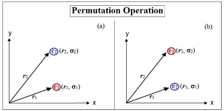
Figure 1: Vector description of the permutation operation of the electronic coordinates. (a) The coordinates before switching are spatial ${\bf{r}}_{1}$ and spin $\sigma_{1}$ coordinates for electron 1, and spatial ${\bf{r}}_{2}$ and spin $\sigma_{2}$ coordinates for electron 2; thus $e_{1}({\bf{r}}_{1},\sigma_{1})$ and $e_{2}({\bf{r}}_{2},\sigma_{2})$. (b) As a result of switching both the spatial and spin coordinates for each electron the new coordinates are spatial ${\bf{r}}_{2}$ and spin $\sigma_{2}$ coordinates for electron 1, and spatial ${\bf{r}}_{1}$ and spin $\sigma_{1}$ coordinates for electron 2; thus $e_{1}({\bf{r}}_{2},\sigma_{2})$ and $e_{2}({\bf{r}}_{1},\sigma_{1})$.

The permutation operation $P_{12}$ permutes the coordinates ${\bf{x}}_{1},{\bf{x}}_{2}$ of the electrons $1$ and $2$. Fig 1 is a $2$D vector description of the switching of the electronic coordinates. Fig. 1(a) corresponds to the initial coordinates of the two electrons, and Fig. 1(b) to the switched coordinates.

The corresponding permutation operator $\hat{P}_{12}$ commutes with the Hamiltonian $\hat{H}$:

$$[\hat{P}_{12},\hat{H}]=0,$$ (11)

so that the eigenfunctions of $\hat{H}$ with eigenvalue $E$ (Eq. (1)) are also eigenfunctions of the operator $\hat{P}_{12}$. The action of the operator $\hat{P}_{12}$ on $\Psi({\bf{x}}_{1},{\bf{x}}_{2})$ is thus

$$\hat{P}_{12}\Psi({\bf{x}}_{1},{\bf{x}}_{2})=\Psi({\bf{x}}_{2},{\bf{x}}_{1}).$$ (12)

Operating with $\hat{P}_{12}$ on Eq. (12) one obtains

$$\hat{P}_{12}\hat{P}_{12}\Psi({\bf{x}}_{1},{\bf{x}}_{2})=\Psi({\bf{x}}_{1},{\bf{x}}_{2}),$$ (13)

so that

$$\hat{P}_{12}^{2}=\hat{I},$$ (14)

with $\hat{I}$ the unit operator. Therefore the eigenvalues of the operator $\hat{P}_{12}$ are $\epsilon=\pm 1$. The eigenfunctions that correspond to the eigenvalue $\epsilon=-1$ are such that

$$\hat{P}_{12}\Psi({\bf{x}}_{1},{\bf{x}}_{2})=\Psi({\bf{x}}_{2},{\bf{x}}_{1})=(-1)\Psi({\bf{x}}_{1},{\bf{x}}_{2})$$ (15)

are antisymmetric under the permutation $P_{12}$. This is the statement of the Pauli principle:

$$\Psi\big{[}e_{1}({\bf{r}}_{1}\sigma_{1}),e_{2}({\bf{r}}_{2}\sigma_{2})\big{]}=-\Psi\big{[}e_{1}({\bf{r}}_{2}\sigma_{2}),e_{2}({\bf{r}}_{1}\sigma_{1})\big{]}.$$ (16)

This statement is independent of the analytical structure or symmetry of the binding potential. It is independent of dimensionality. It is valid for arbitrary state. For wave functions of the form of Eq. (7), the statement of the Pauli principle is

$$\psi({\bf{r}}_{1},{\bf{r}}_{2})\chi(\sigma_{1},\sigma_{2})=-\psi({\bf{r}}_{2},{\bf{r}}_{1})\chi(\sigma_{2},\sigma_{1}).$$ (17)

A pictorial description of the Pauli principle for the excited singlet $2^{1}S$ and triplet $2^{3}S$ states of a quantum dot follows:

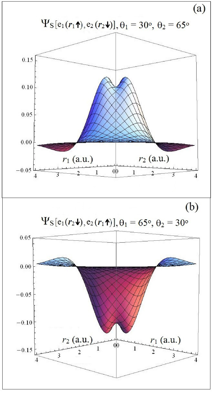
Figure 2: Satisfaction of the Pauli principle for the singlet $2^{1}S$ state wave function of the ‘artificial atom’: (a) $\Psi_{S}[e_{1}({\bf{r}}_{1}{\boldsymbol{\uparrow}})$, $e_{2}({\bf{r}}_{2}{\boldsymbol{\downarrow}})](\theta_{1}=30^{\circ},\theta_{2}=65^{\circ})$ ; (b) $\Psi_{S}[e_{1}({\bf{r}}_{2}{\boldsymbol{\downarrow}})$, $e_{2}({\bf{r}}_{1}{\boldsymbol{\uparrow}})](\theta_{1}=65^{\circ},\theta_{2}=30^{\circ})$. (Note the switch of the coordinate axes labels in Fig. 2(b).)

Singlet $2^{1}S$ state: Employing the exact analytical expression for the excited singlet state of the ‘artificial atom’ or quantum dot as given in the Appendix Eq. (A2), the wave function $\Psi_{S}[e_{1}({\bf{r}}_{1}{\boldsymbol{\uparrow}}),e_{2}({\bf{r}}_{2}{\boldsymbol{\downarrow}})](\theta_{1}=30^{\circ},\theta_{2}=65^{\circ})$ is plotted in Fig. 2(a). (This corresponds to the case of Fig. 1(a).) The plot for the wave function when the coordinates are switched, (corresponding to Fig. 1 (b)), which is $\Psi_{S}[e_{1}({\bf{r}}_{2}{\boldsymbol{\downarrow}}),e_{2}({\bf{r}}_{1}{\boldsymbol{\uparrow}})](\theta_{1}=65^{\circ},\theta_{2}=30^{\circ})$ is given in Fig. 2(b). (Note the switching of the coordinate axes labels in Fig. 2(b).) The satisfaction of the Pauli principle of Eq. (16) is evident.

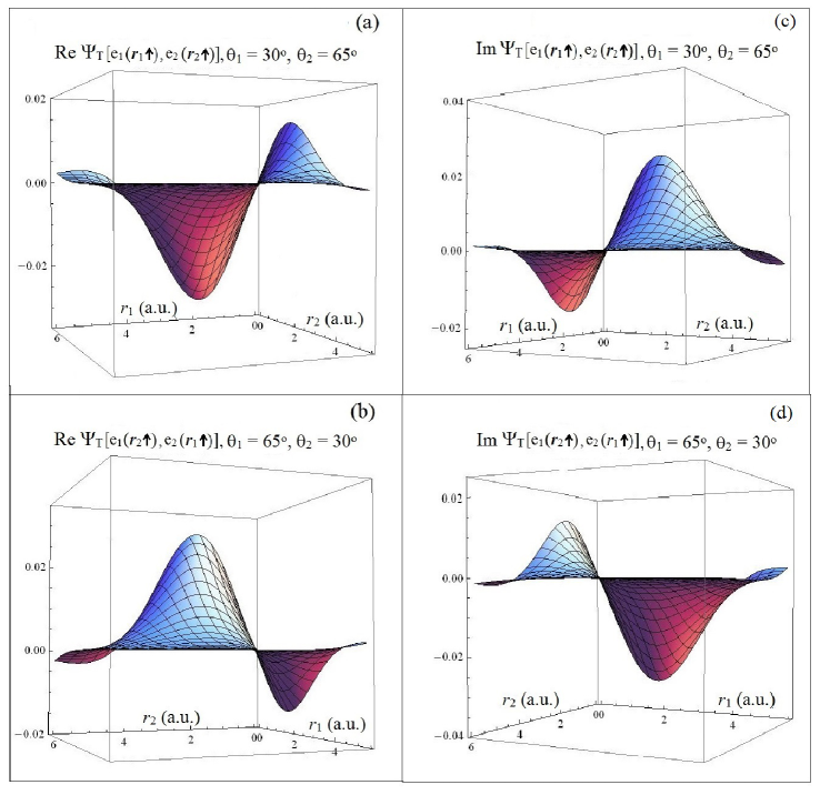
Figure 3: Satisfaction of the Pauli principle for the Real and Imaginary parts of the triplet $2^{3}S$ state wave function for the ‘artificial atom’: (a) $\Re\Psi_{T}[e_{1}({\bf{r}}_{1}{\boldsymbol{\uparrow}}),e_{2}({\bf{r}}_{2}{\boldsymbol{\uparrow}})](\theta_{1}=30^{\circ},\theta_{2}=65^{\circ})$ ; (b) $\Re\Psi_{T}[e_{1}({\bf{r}}_{2}{\boldsymbol{\uparrow}}),e_{2}({\bf{r}}_{1}{\boldsymbol{\uparrow}})]$ $(\theta_{1}=65^{\circ},\theta_{2}=30^{\circ})$. (Note the switching of the coordinate axes labels In Fig. 3(b).) (c) $\Im\Psi_{T}[e_{1}({\bf{r}}_{1}{\boldsymbol{\uparrow}}),e_{2}({\bf{r}}_{2}{\boldsymbol{\uparrow}})]$ $(\theta_{1}=30^{\circ},\theta_{2}=65^{\circ})$; (d) $\Im\Psi_{T}[e_{1}({\bf{r}}_{2}{\boldsymbol{\uparrow}}),e_{2}({\bf{r}}_{1}{\boldsymbol{\uparrow}})]$ $(\theta_{1}=65^{\circ},\theta_{2}=30^{\circ})$. (Note the switching of the coordinate axes labels in Fig. 3(d).)

Triplet $2^{3}S$ state: Employing the exact analytical expression for the triplet state wave function for the ‘artificial atom’ given in the Appendix by Eq. (A3), the Real part of the wave function $\Re\Psi_{T}[e_{1}({\bf{r}}_{1}{\boldsymbol{\uparrow}}),e_{2}({\bf{r}}_{2}{\boldsymbol{\uparrow}})](\theta_{1}=30^{\circ},\theta_{2}=65^{\circ})$ is plotted in Fig. 3(a). The Real part of the wave function with the switched coordinates $\Re\Psi_{T}[e_{1}({\bf{r}}_{2}{\boldsymbol{\uparrow}}),e_{2}({\bf{r}}_{1}{\boldsymbol{\uparrow}})](\theta_{1}=65^{\circ},\theta_{2}=30^{\circ})$ is plotted in Fig. 3(b). In Figs 3(c) and 3(d), the Imaginary parts of the wave function $\Im\Psi_{T}[e_{1}({\bf{r}}_{1}{\boldsymbol{\uparrow}}),e_{2}({\bf{r}}_{2}{\boldsymbol{\uparrow}})](\theta_{1}=30^{\circ},\theta_{2}=65^{\circ})$ and $\Im\Psi_{T}[e_{1}({\bf{r}}_{2}{\boldsymbol{\uparrow}}),e_{2}({\bf{r}}_{1}{\boldsymbol{\uparrow}})](\theta_{1}=65^{\circ},\theta_{2}=30^{\circ})$, respectively, are plotted. (Note the switching of the coordinate axes labels in Figs. 3(b) and 3(d), respectively.) The satisfaction of the Pauli principle of Eq. (16) by the Real and Imaginary parts of the wave function is evident.

III New Symmetry Operation and Wave Function Identity

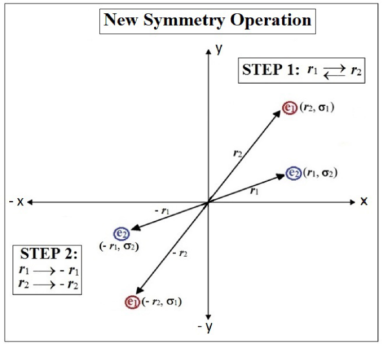
Figure 4: Vector description to illustrate the new symmetry operation. The original electronic coordinates are those described in Fig. 1 (a). The symmetry operation is a two-step process. STEP 1 (quadrant 1): The spatial coordinates are interchanged while the spin coordinates remain unchanged which results in spatial ${\bf{r}}_{2}$ and spin $\sigma_{1}$ coordinates for electron 1, and spatial ${\bf{r}}_{1}$ and spin $\sigma_{2}$ coordinates for electron 2; thus $e_{1}({\bf{r}}_{2},\sigma_{1})$ and $e_{2}({\bf{r}}_{1},\sigma_{2})$. STEP 2 (quadrant 3) is an inversion about the origin. Thus the final result is spatial $-{\bf{r}}_{2}$ and spin $\sigma_{1}$ coordinates for electron 1, and spatial $-{\bf{r}}_{1}$ and spin $\sigma_{2}$ coordinates for electron 2; hence $e_{1}(-{\bf{r}}_{2},\sigma_{1})$ and $e_{2}(-{\bf{r}}_{1},\sigma_{2})$.

With the initial coordinates of the electrons as exhibited in Fig. 1(a), the new symmetry operation $O_{sym}$ is a two-step process on the electron coordinates as explained in Fig. 4. In Step 1 the spatial coordinates of the electrons are switched $({\bf{r}}_{1}\leftrightarrow{\bf{r}}_{2})$ while keeping the spin coordinates associated with each electron unchanged (see quadrant 1). Step 2 is an inversion through the center of symmetry $({\bf{r}}_{1}\rightarrow-{\bf{r}}_{1}~{}\mbox{and}~{}{\bf{r}}_{2}\rightarrow-{\bf{r}}_{2})$ while the spin coordinates remain unchanged (see quadrant 3).

The operator $\hat{O}_{sym}$ corresponding to the symmetry operation $O_{sym}$ commutes with the Hamiltonian $\hat{H}$:

$$\big{[}\hat{O}_{sym},\hat{H}\big{]}=0,$$ (18)

so that the eigenfunctions of $\hat{O}_{sym}$ are the same as those of the Hamiltonian $\hat{H}$. Operating with the operator $\hat{O}_{sym}$ on the wave function $\Psi({\bf{x}}_{1},{\bf{x}}_{2})$ one obtains

$$\hat{O}_{sym}\Psi\big{[}e_{1}({\bf{r}}_{1}\sigma_{1}),e_{2}({\bf{r}}_{2}\sigma_{2})\big{]}=\Psi\big{[}e_{1}(-{\bf{r}}_{2}\sigma_{1}),e_{2}(-{\bf{r}}_{1}\sigma_{2})\big{]}.$$ (19)

Operating with $\hat{O}_{sym}$ a second time leads to

$$\hat{O}_{sym}\hat{O}_{sym}\Psi\big{[}e_{1}({\bf{r}}_{1}\sigma_{1}),e_{2}({\bf{r}}_{2}\sigma_{2})\big{]}=\Psi\big{[}e_{1}({\bf{r}}_{1}\sigma_{1}),e_{2}({\bf{r}}_{2}\sigma_{2})\big{]},$$ (20)

so that

$$\hat{O}_{sym}^{2}=\hat{I}.$$ (21)

Thus, the eigenvalues of the operator $\hat{O}_{sym}$ are $\lambda=\pm 1$. The wave functions that correspond to the eigenvalue $\lambda=+1$ are such that

$$\hat{O}_{sym}\Psi\big{[}e_{1}({\bf{r}}_{1}\sigma_{1}),e_{2}({\bf{r}}_{2}\sigma_{2})\big{]}=(+1)\Psi\big{[}e_{1}({\bf{r}}_{1}\sigma_{1}),e_{2}({\bf{r}}_{2}\sigma_{2})\big{]}.$$ (22)

The equality of the symmetry transformed wave function to the wave function is referred to as the Wave Function Identity:

$$\Psi\big{[}e_{1}({\bf{r}}_{1}\sigma_{1}),e_{2}({\bf{r}}_{2}\sigma_{2})\big{]}=\Psi\big{[}e_{1}(-{\bf{r}}_{2}\sigma_{1}),e_{2}(-{\bf{r}}_{1}\sigma_{2})\big{]}.$$ (23)

In terms of the wave function $\Psi({\bf{x}}_{1},{\bf{x}}_{2})$ of Eq. (7), the Wave Function Identity statement is

$$\psi({\bf{r}}_{1},{\bf{r}}_{2})\chi(\sigma_{1},\sigma_{2})=\psi(-{\bf{r}}_{2},-{\bf{r}}_{1})\chi(\sigma_{1},\sigma_{2}).$$ (24)

The Wave Function Identity is valid only for binding potentials $v({\bf{r}})$ that are even. In common with the Pauli principle, it is valid for binding potentials of arbitrary analytical structure, and arbitrary dimensionality. It is also valid for both singlet and triplet states.

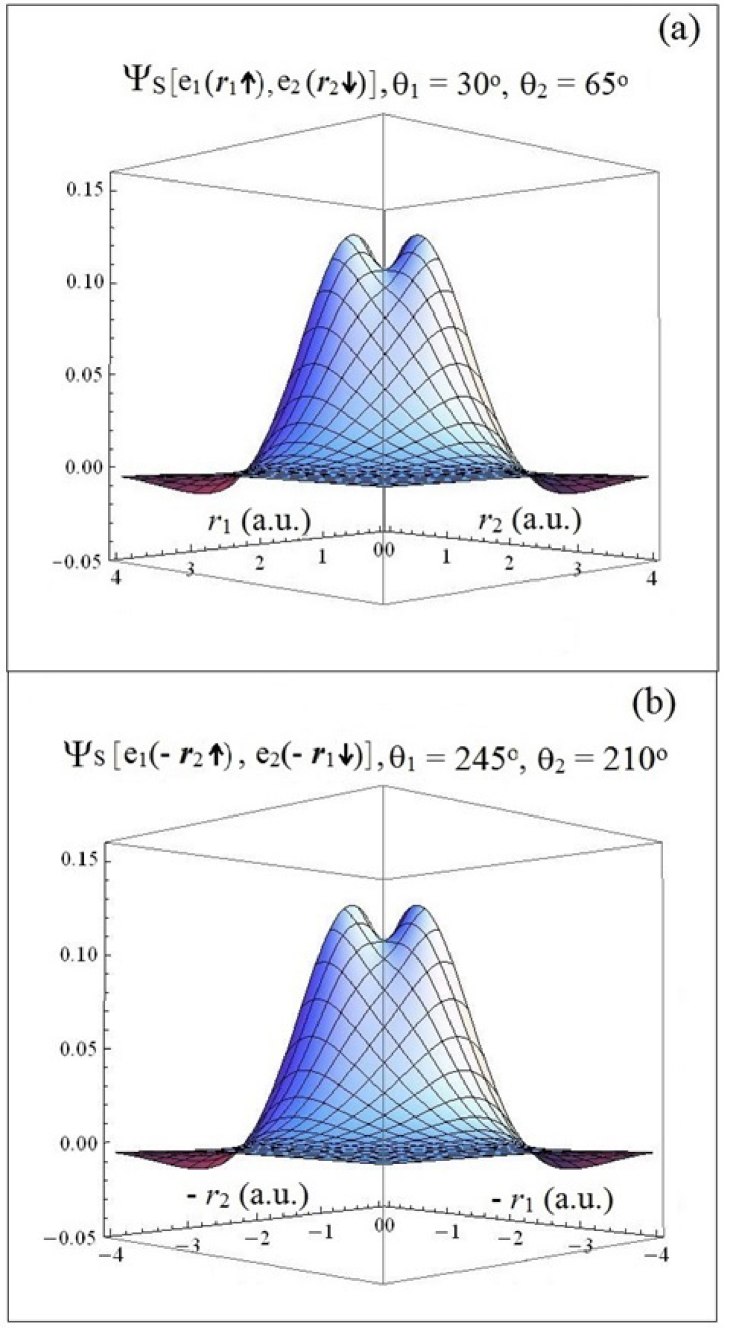
Figure 5: Satisfaction of the Wave Function Identity for the singlet $2^{1}S$ state of the ‘artificial atom’: (a) $\Psi_{S}[e_{1}({\bf{r}}_{1}{\boldsymbol{\uparrow}}),e_{2}({\bf{r}}_{2}{\boldsymbol{\downarrow}})]$ $(\theta_{1}=30^{\circ},\theta_{2}=65^{\circ})$ and (b) $\Psi_{S}[e_{1}(-{\bf{r}}_{2}{\boldsymbol{\uparrow}}),e_{2}(-{\bf{r}}_{1}{\boldsymbol{\downarrow}})]$ $(\theta_{1}=245^{\circ},\theta_{2}=210^{\circ})$.

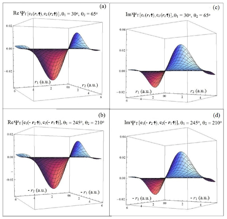
Figure 6: Satisfaction of the Wave Function Identity for the Real and Imaginary parts of the triplet $2^{3}S$ state of the ‘artificial atom’: (a) $\Re\Psi_{T}[e_{1}({\bf{r}}_{1}{\boldsymbol{\uparrow}}),e_{2}({\bf{r}}_{2}{\boldsymbol{\uparrow}})]$ $(\theta_{1}=30^{\circ},\theta_{2}=65^{\circ})$ and (b) $\Re\Psi_{T}[e_{1}(-{\bf{r}}_{2}{\boldsymbol{\uparrow}}),e_{2}(-{\bf{r}}_{1}{\boldsymbol{\uparrow}})]$ $(\theta_{1}=245^{\circ},\theta_{2}=210^{\circ})$ and (c) $\Im\Psi_{T}[e_{1}({\bf{r}}_{1}{\boldsymbol{\uparrow}}),e_{2}({\bf{r}}_{2}{\boldsymbol{\uparrow}})]$ $(\theta_{1}=30^{\circ},\theta_{2}=65^{\circ})$ and (d) $\Im\Psi_{T}[e_{1}(-{\bf{r}}_{2}{\boldsymbol{\uparrow}}),e_{2}(-{\bf{r}}_{1}{\boldsymbol{\uparrow}})]$ $(\theta_{1}=245^{\circ},\theta_{2}=210^{\circ})$.

A pictorial representation of the Wave Function Identity for the singlet and triplet states of a quantum dot is provided in Figs. 5 and 6.

Singlet $2^{1}S$ state: The Wave Function Identity of Eq. (23) is exhibited in Fig. 5. In Figs. 5(a) and 5(b), respectively, the wave functions $\Psi_{S}[e_{1}({\bf{r}}_{1}{\boldsymbol{\uparrow}}),e_{2}({\bf{r}}_{2}{\boldsymbol{\downarrow}})](\theta_{1}=30^{\circ},\theta_{2}=65^{\circ})$ and $\Psi_{S}[e_{1}(-{\bf{r}}_{2}{\boldsymbol{\uparrow}}),e_{2}(-{\bf{r}}_{1}{\boldsymbol{\downarrow}})](\theta_{1}=245^{\circ},\theta_{2}=210^{\circ})$ for the ‘artificial atom’ are plotted. (Note the change in the labels of the coordinate axes in Fig. 5(b).) The satisfaction of the Wave Function Identity is evident.

Triplet $2^{3}S$ state: In Figs. 6(a) and (b), respectively, the Real part of the triplet state wave functions for the ‘artificial atom’ $\Re\Psi_{T}[e_{1}({\bf{r}}_{1}{\boldsymbol{\uparrow}}),e_{2}({\bf{r}}_{2}{\boldsymbol{\uparrow}})](\theta_{1}=30^{\circ},\theta_{2}=65^{\circ})$ and $\Re\Psi_{T}[e_{1}(-{\bf{r}}_{2}{\boldsymbol{\uparrow}}),e_{2}(-{\bf{r}}_{1}{\boldsymbol{\uparrow}})](\theta_{1}=245^{\circ},\theta_{2}=210^{\circ})$ are plotted. In Figs. 6(c) and (d), the Imaginary part of the wave functions $\Im\Psi_{T}[e_{1}({\bf{r}}_{1}{\boldsymbol{\uparrow}}),e_{2}({\bf{r}}_{2}{\boldsymbol{\uparrow}})](\theta_{1}=30^{\circ},\theta_{2}=65^{\circ})$ and $\Im\Psi_{T}[e_{1}(-{\bf{r}}_{2}{\boldsymbol{\uparrow}}),e_{2}(-{\bf{r}}_{1}{\boldsymbol{\uparrow}})](\theta_{1}=245^{\circ},\theta_{2}=210^{\circ})$ are plotted. (Note the change in the labels of the coordinate axes in Figs. 6(b) and 6(d).)These figures demonstrate the satisfaction of the Wave Function Identity for the Real and Imaginary parts of the wave function for the triplet state.

IV Parity of Singlet and Triplet State Wave Functions

We next show by application of the permutation operator $\hat{P}_{12}$ to the Wave Function Identity that the parity of the singlet states is even, and that of the triplet states odd. To do so, consider the form of the wave function $\Psi({\bf{x}}_{1},{\bf{x}}_{2})$ to be that of Eq. (7). We know from the previous section that

$$\hat{O}_{sym}\big{[}\psi({\bf{r}}_{1},{\bf{r}}_{2})\chi(\sigma_{1},\sigma_{2})\big{]}=\psi(-{\bf{r}}_{2},-{\bf{r}}_{1})\chi(\sigma_{1},\sigma_{2}).$$ (25)

On application of the permutation operator $\hat{P}_{12}$ to Eq. (25), we have

$$\hat{P}_{12}\hat{O}_{sym}\big{[}\psi({\bf{r}}_{1},{\bf{r}}_{2})\chi(\sigma_{1},\sigma_{2})\big{]}=-\psi(-{\bf{r}}_{1},-{\bf{r}}_{2})\chi(\sigma_{2},\sigma_{1}).$$ (26)

(Note that the negative sign on the right is a consequence of the Pauli principle.) Let us consider the singlet and triplet states separately.

Singlet $2^{1}S$ state: For the singlet state $\Psi_{S}({\bf{x}}_{1},{\bf{x}}_{2})$, the spin component of the wave function $\chi_{S}(\sigma_{1},\sigma_{2})$ is antisymmetric in an interchange of the spin coordinates. Hence, the spatial component $\psi_{S}({\bf{r}}_{1},{\bf{r}}_{2})$ is symmetric in an interchange of the spatial coordinates. Employing these constraints, we then have from Eq. (24)

$$\hat{P}_{12}\hat{O}_{sym}\big{[}\psi_{S}({\bf{r}}_{1},{\bf{r}}_{2})\chi_{S}(\sigma_{1},\sigma_{2})\big{]} = -\psi_{S}(-{\bf{r}}_{1},-{\bf{r}}_{2})\chi_{S}(\sigma_{2},\sigma_{1})$$ (27)

$$= \big{[}-\psi_{S}(-{\bf{r}}_{1},-{\bf{r}}_{2})\big{]}\big{[}-\chi_{S}(\sigma_{1},\sigma_{2})\big{]}$$ (28)

$$= \psi_{S}(-{\bf{r}}_{1},-{\bf{r}}_{2})\chi_{S}(\sigma_{1},\sigma_{2})$$ (29)

$$= \psi_{S}(-{\bf{r}}_{2},-{\bf{r}}_{1})\chi_{S}(\sigma_{1},\sigma_{2}).$$ (30)

From a comparison of the Wave Function Identity of Eq. (24) to that of Eq. (30), together with Eq. (29), it follows that for the singlet state

$$\psi_{S}({\bf{r}}_{1},{\bf{r}}_{2})\chi(\sigma_{1},\sigma_{2})=\psi_{S}(-{\bf{r}}_{1},-{\bf{r}}_{2})\chi_{S}(\sigma_{1},\sigma_{2})$$ (31)

or more generally

$$\Psi_{S}({\bf{x}}_{1},{\bf{x}}_{2})=\Psi_{S}(-{\bf{x}}_{1},-{\bf{x}}_{2}),$$ (32)

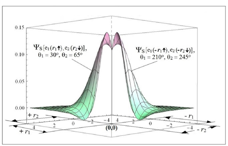
Figure 7: Even Parity of the singlet $2^{1}S$ state wave function of the ‘artificial atom’. The functions $\Psi_{S}[e_{1}({\bf{r}}_{1}{\boldsymbol{\uparrow}}),e_{2}({\bf{r}}_{2}{\boldsymbol{\downarrow}})]$ $(\theta_{1}=30^{\circ},\theta_{2}=65^{\circ})$ and $\Psi_{S}[e_{1}(-{\bf{r}}_{1}{\boldsymbol{\uparrow}}),e_{2}(-{\bf{r}}_{2}{\boldsymbol{\downarrow}})]$ $(\theta_{1}=210^{\circ},\theta_{2}=245^{\circ})$ are plotted.

where $-{\bf{x}}=-{\bf{r}}\sigma$. The right hand side of Eq. (31) corresponds to an inversion about the center of symmetry, and thus the singlet state has even parity. In Fig. 7 we demonstrate the even parity of the singlet state wave function for the ‘artificial atom’ by plotting $\Psi_{S}[e_{1}({\bf{r}}_{1}{\boldsymbol{\uparrow}}),e_{2}({\bf{r}}_{2}{\boldsymbol{\downarrow}})](\theta_{1}=30^{\circ};\theta_{2}=65^{\circ})$ and $\Psi_{S}[e_{1}(-{\bf{r}}_{1}{\boldsymbol{\uparrow}}),e_{2}(-{\bf{r}}_{2}{\boldsymbol{\downarrow}})](\theta_{1}=210^{\circ};\theta_{2}=245^{\circ})$.

Triplet $2^{3}S$ state: For the triplet state, the spin component of the wave function $\chi_{T}(\sigma_{1},\sigma_{2})$ is symmetric in an interchange of the spin coordinates, and therefore the spatial component $\psi_{T}({\bf{r}}_{1},{\bf{r}}_{2})$ is antisymmetric in an interchange of the spatial coordinates. Employing these constraints, we then have from Eq. (26)

$$\hat{P}_{12}\hat{O}_{sym}\big{[}\psi_{T}({\bf{r}}_{1},{\bf{r}}_{2})\chi_{T}(\sigma_{1},\sigma_{2})\big{]} = -\psi_{T}(-{\bf{r}}_{1},-{\bf{r}}_{2})\chi_{T}(\sigma_{2},\sigma_{1})$$ (33)

$$= -\psi_{T}(-{\bf{r}}_{1},-{\bf{r}}_{2})\chi_{T}(\sigma_{1},\sigma_{2})$$ (34)

$$= -[-\psi_{T}(-{\bf{r}}_{2},-{\bf{r}}_{1})]\chi_{T}(\sigma_{1},\sigma_{2})$$ (35)

$$= \psi_{T}(-{\bf{r}}_{2},-{\bf{r}}_{1})\chi_{T}(\sigma_{1},\sigma_{2}).$$ (36)

From a comparison of the Wave Function Identity of Eq. (24) to that of Eq. (36), together with Eq. (34), it follows that for the triplet state

$$\psi_{T}({\bf{r}}_{1},{\bf{r}}_{2})\chi(\sigma_{1},\sigma_{2})=-\psi_{T}(-{\bf{r}}_{1},-{\bf{r}}_{2})\chi_{T}(\sigma_{1},\sigma_{2})$$ (37)

or more generally

$$\Psi_{T}({\bf{x}}_{1},{\bf{x}}_{2})=-\Psi_{T}(-{\bf{x}}_{1},-{\bf{x}}_{2}).$$ (38)

Since on inversion, the wave function changes sign, the parity of the triplet states is odd.

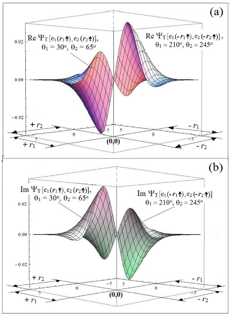
Figure 8: Odd Parity of the Real and Imaginary parts of the triplet $2^{3}S$ wave function for the ‘artificial atom’. The following functions are plotted (a)$\Re\Psi_{T}[e_{1}({\bf{r}}_{1}{\boldsymbol{\uparrow}}),e_{2}({\bf{r}}_{2}{\boldsymbol{\uparrow}})](\theta_{1}=30^{\circ},\theta_{2}=65^{\circ})$ and $\Re\Psi_{T}[e_{1}(-{\bf{r}}_{1}{\boldsymbol{\uparrow}}),e_{2}(-{\bf{r}}_{2}{\boldsymbol{\uparrow}})](\theta_{1}=210^{\circ},\theta_{2}=245^{\circ})$; (b) $\Im\Psi_{T}[e_{1}({\bf{r}}_{1}{\boldsymbol{\uparrow}}),e_{2}({\bf{r}}_{2}{\boldsymbol{\uparrow}})](\theta_{1}=30^{\circ},\theta_{2}=65^{\circ})$ and $\Im\Psi_{T}[e_{1}(-{\bf{r}}_{1}{\boldsymbol{\uparrow}}),e_{2}(-{\bf{r}}_{2}{\boldsymbol{\uparrow}})](\theta_{1}=210^{\circ},\theta_{2}=245^{\circ})$.

To exhibit the odd parity of the triplet state wave function, we plot in Fig. 8(a) $\Re\Psi_{T}[e_{1}({\bf{r}}_{1}{\boldsymbol{\uparrow}}),e_{2}({\bf{r}}_{2}{\boldsymbol{\uparrow}})](\theta_{1}=30^{\circ},\theta_{2}=65^{\circ})$ and $\Re\Psi_{T}[e_{1}(-{\bf{r}}_{1}{\boldsymbol{\uparrow}}),e_{2}(-{\bf{r}}_{2}{\boldsymbol{\uparrow}})](\theta_{1}=210^{\circ},\theta_{2}=245^{\circ})$ . In Fig. 8(b) we plot $\Im\Psi_{T}[e_{1}({\bf{r}}_{1}{\boldsymbol{\uparrow}}),e_{2}({\bf{r}}_{2}{\boldsymbol{\uparrow}})](\theta_{1}=30^{\circ},\theta_{2}=65^{\circ})$ and $\Im\Psi_{T}[e_{1}(-{\bf{r}}_{1}{\boldsymbol{\uparrow}}),e_{2}(-{\bf{r}}_{2}{\boldsymbol{\uparrow}})](\theta_{1}=210^{\circ},\theta_{2}=245^{\circ})$.

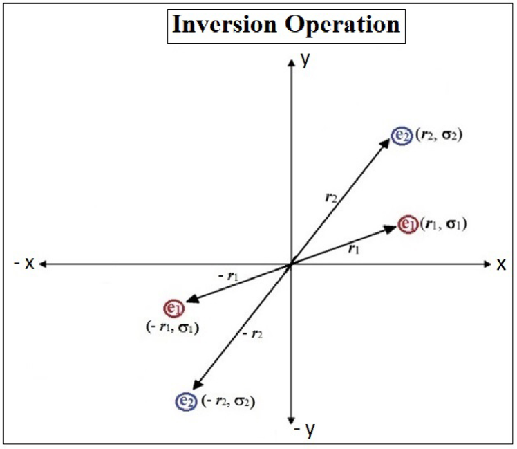
Figure 9: Vector description of the inversion operation. The figure is valid for both the singlet and triplet states. Quadrant 1 is the same as Fig. 1 (a). Quadrant 3: Electron 1 with spatial $-{\bf{r}}_{1}$ and spin $\sigma_{1}$ coordinates: $e_{1}(-{\bf{r}}_{1},\sigma_{1})$; Electron 2 with spatial $-{\bf{r}}_{2}$ and spin $\sigma_{2}$ coordinates: $e_{2}(-{\bf{r}}_{2},\sigma_{2})$.

It is evident from the above that the symmetry operation $O_{sym}$ followed by a permutation $P_{12}$ is equivalent to an inversion (see Fig. 9). In operator form,

$$\hat{P}_{12}\hat{O}_{sym}=\hat{\Pi},$$ (39)

where $\hat{\Pi}$ is the parity operator. The properties of the parity operator are the following: $[\hat{\Pi},\hat{H}]=0$; $\hat{\Pi}^{2}=\hat{I}$; the eigenvalues of $\hat{\Pi}$ are $\alpha=\pm 1$.

As a consequence of Eqs. (32), (38), (39), we conclude that the eigenfunctions of the parity operator for eigenvalue $\alpha=1$ are singlet states, and those of the eigenvalue $\alpha=-1$ are triplet states. Thus,

$$\hat{P}_{12}\hat{O}_{sym}\Psi_{S}({\bf{r}}_{1}\sigma_{1},{\bf{r}}_{2}\sigma_{2})=\hat{\Pi}\Psi_{S}({\bf{r}}_{1}\sigma_{1},{\bf{r}}_{2}\sigma_{2})=\Psi_{S}(-{\bf{r}}_{1}\sigma_{1},{-\bf{r}}_{2}\sigma_{2}),$$ (40)

and

$$\hat{P}_{12}\hat{O}_{sym}\Psi_{T}({\bf{r}}_{1}\sigma_{1},{\bf{r}}_{2}\sigma_{2})=\hat{\Pi}\Psi_{T}({\bf{r}}_{1}\sigma_{1},{\bf{r}}_{2}\sigma_{2})=-\Psi_{T}(-{\bf{r}}_{1}\sigma_{1},{-\bf{r}}_{2}\sigma_{2}).$$ (41)

Note that a priori it is not known that the positive eigenvalue of the parity operator $\hat{\Pi}$ corresponds to the singlet state, whereas the negative eigenvalue that of the triplet state. It is only a posteriori, that is following the proof that the parity of singlet states is even and that of triplet states odd, that one can associate the positive eigenvalue of the parity operator $\hat{\Pi}$ with singlet states and the negative eigenvalue with the triplet state.

V Parity about all Points of Electron-Electron Coalescence

As explained in the Introduction, one may conclude from the electron-electron coalescence condition of Eq.(8), that the singlet states satisfy the cusp coalescence constraint whereas the triplet states satisfy the node coalescence condition. In other words, the singlet state wave functions exhibit a cusp at all points of electron-electron coalescence, and triplet states exhibit a node at these points. We have also proved that the singlet states have even parity and the triplet states odd parity. The parity of a wave function is with respect to the center (origin) of the system as defined by the symmetrical binding potential. Now the origin of the system also constitutes a point of electron-electron coalescence. Thus for singlet states, the cusp at the origin must be such that the slope of the wave function as the origin is approached from the right must be the same but the negative of the slope when approached from the left. The slopes have a discontinuity at the origin. From the perspective of the coalescence of electrons, the origin is not a special point of configuration space. There is no reason why the parity about all other points of electron-electron coalescence should not also be the same. Hence, it follows that the parity of the singlet state wave functions at all points of electron-electron coalescence is even.

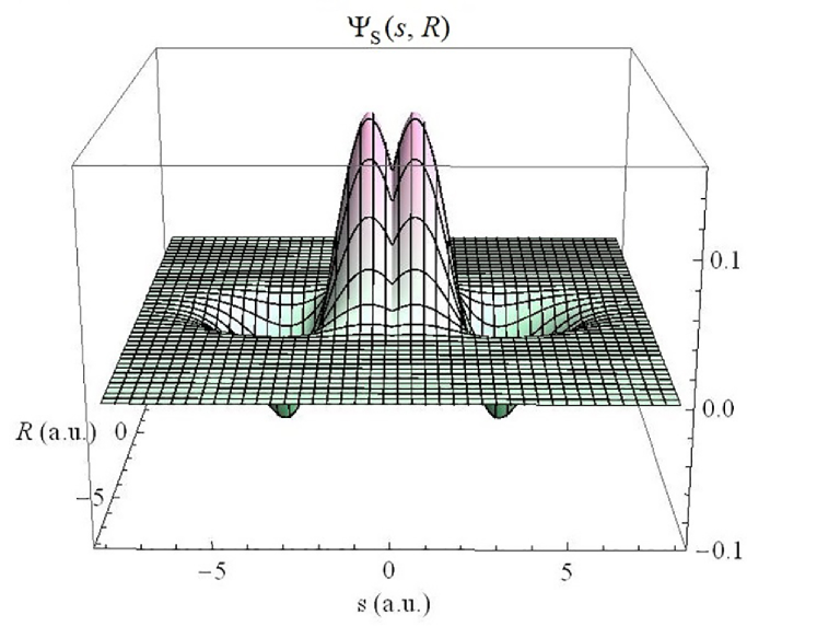
Figure 10: The singlet $2^{1}S$ state wave function of the ‘artificial atom’ plotted as a function of the center of mass ${\bf{R}}$ and relative ${\bf{s}}$ coordinates.

To show that this is the case, we plot in Fig. 10 the singlet $2^{1}S$ state wave function of the ‘artificial atom’ as a function of the center of mass ${\bf{R}}=({\bf{r}}_{1}+{\bf{r}}_{2})/2$ and relative ${\bf{s}}={\bf{r}}_{2}-{\bf{r}}_{1}$ coordinates. As may be observed from the figure, the parity of the wave function about the line ${\bf{s}}=0$ is even.

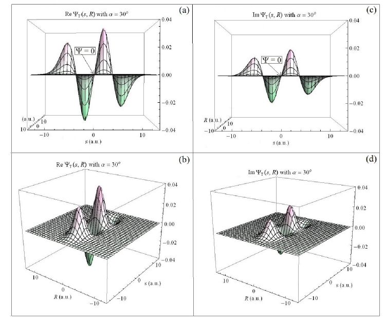
Figure 11: Two views of the Real (a), (b) and Imaginary (c), (d) parts of the triplet $2^{3}S$ wave function for the ‘artificial atom’ plotted as a function of the center of mass ${\bf{R}}$ and relative ${\bf{s}}$ coordinates for $\alpha=30^{\circ}$, where $\alpha$ is the angle of the relative coordinate ${\bf{s}}$.

The triplet state wave functions exhibit a node at the origin, and have odd parity. Hence, the functions are smooth, i.e. continuous and with continuous first derivatives, about the origin. Again, the origin corresponds to just one point of electron-electron coalescence. Thus, one may conclude that triplet state wave functions have odd parity about all points of electron-electron coalescence. In Fig. 11 (a) and (b), we plot two views of the Real part of the triplet $2^{3}S$ state wave function of the ‘artificial atom’ as a function of the coordinates $({\bf{s}},{\bf{R}})$ for $\alpha=30^{\circ}$, where $\alpha$ is the angle of the relative coordinate. Observe that the parity of the wave function about the line ${\bf{s}}=0$ is odd. In Fig. 11 (c) and (d), two views of the Imaginary part of the wave function are plotted. Again, the parity about the line ${\bf{s}}=0$ is odd.

Finally, implicit in the understanding that the singlet state wave functions have even parity is that they satisfy the cusp electron-electron coalescence constraint. This too is evident in Fig. 10 for all points ${\bf{s}}=0$. The fact that triplet states have odd parity then implies that these wave functions satisfy the node coalescence condition. This is evident for both the Real and Imaginary parts of the triplet state wave function in Fig. 11 along the ${\bf{s}}=0$ line.

VI Proof of Satisfaction of the Wave Function Identity by the Exact Wave Function

In this section we prove that the exact wave function of any $2$-electron system with symmetrical binding potential $v({\bf{r}})$ must satisfy the Wave Function Identity. The examples of the previous section show that this is the case for the $2$D ‘artificial atoms’ with symmetric harmonic binding potential. This is also the case for $3$D ‘artificial atoms’ with the magnetic field absent. This can be seen from the solutions of the corresponding Schrödinger equations which can also be obtained exactly in closed analytical form 22 ; 23 ; 34 ; 35 ; 36 ; 37 ; 38 ; 39 . Here we prove the result for arbitrary symmetrical potential $v({\bf{r}})$ and arbitrary interaction of the form $w(|{\bf{r}}-{\bf{r}}^{\prime}|)$.

The exact wave function $\Psi({\bf{x}}_{1},{\bf{x}}_{2})$ of Eq. (7) may be written as

$$\Psi({\bf{x}}_{1},{\bf{x}}_{2})=\bigg{[}\sum_{i}c_{i}\Phi_{i}({\bf{r}}_{1},{\bf{r}}_{2})\bigg{]}\chi(\sigma_{1},\sigma_{2}),$$ (42)

so that the spatial part $\psi({\bf{r}}_{1},{\bf{r}}_{2})$ is given by the infinite series expansion

$$\psi({\bf{r}}_{1},{\bf{r}}_{2})=\sum_{i}c_{i}\Phi_{i}({\bf{r}}_{1},{\bf{r}}_{2}),$$ (43)

where the determinantal functions $\Phi_{i}({\bf{r}}_{1},{\bf{r}}_{2})$ form a complete orthonormal set, with the coefficients $c_{i}$ being suitably chosen constants. If it is ensured that each determinant $\Phi_{i}({\bf{r}}_{1},{\bf{r}}_{2})$ satisfies the Wave Function Identity, the exact wave function will satisfy the identity.

Triplet States

Since for the triplet state, the spin component of the wave function $\chi(\sigma_{1},\sigma_{2})$ is symmetric in an interchange of the spin coordinates $(\sigma_{1},\sigma_{2})$, each spatial component determinant $\Phi_{i}({\bf{r}}_{1},{\bf{r}}_{2})$ must be antisymmetric in an interchange of the spatial coordinates $({\bf{r}}_{1},{\bf{r}}_{2})$. Thus, an arbitrary determinant $\Phi({\bf{r}}_{1},{\bf{r}}_{2})$ is given as

$$\Phi({\bf{r}}_{1},{\bf{r}}_{2})=\phi_{1}({\bf{r}}_{1})\phi_{2}({\bf{r}}_{2})-\phi_{2}({\bf{r}}_{1})\phi_{1}({\bf{r}}_{2}).$$ (44)

As the binding potential $v({\bf{r}})$ is symmetrical, it is possible to ensure that the orbital $\phi_{1}({\bf{r}})$ has even parity and the orbital $\phi_{2}({\bf{r}})$ has odd parity, i.e.

$$\phi_{1}({\bf{r}})=\phi_{1}(-{\bf{r}})~{};~{}~{}~{}~{}\phi_{2}({\bf{r}})=-\phi_{2}(-{\bf{r}}).$$ (45)

Then, the spatial part of the right hand side of the Wave Function Identity of Eq. (24) (with $\psi(-{\bf{r}}_{2},-{\bf{r}}_{1})$ replaced by $\Phi(-{\bf{r}}_{2},-{\bf{r}}_{1})$) employing Eq. (44) becomes

$$\Phi(-{\bf{r}}_{2},-{\bf{r}}_{1})=\phi_{1}(-{\bf{r}}_{2})\phi_{2}(-{\bf{r}}_{1})-\phi_{2}(-{\bf{r}}_{2})\phi_{1}(-{\bf{r}}_{1}).$$ (46)

On substituting Eq. (45) on the right hand side of Eq. (46), we have

$$\Phi(-{\bf{r}}_{2},-{\bf{r}}_{1}) = \phi_{1}({\bf{r}}_{2})[-\phi_{2}({\bf{r}}_{1})]-[-\phi_{2}({\bf{r}}_{2})]\phi_{1}({\bf{r}}_{1})$$ (47)

$$= \phi_{1}({\bf{r}}_{1})\phi_{2}({\bf{r}}_{2})-\phi_{2}({\bf{r}}_{1})\phi_{1}({\bf{r}}_{2})$$ (48)

$$= \Phi({\bf{r}}_{1},{\bf{r}}_{2}).$$ (49)

This proves that the Wave Function Identity is satisfied for each determinant $\Phi_{i}({\bf{r}}_{1},{\bf{r}}_{2})$ of $\psi({\bf{r}}_{1},{\bf{r}}_{2})$ of Eq. (43), and thereby by the exact triplet state wave function $\Psi({\bf{x}}_{1},{\bf{x}}_{2})$ of Eq. (42).

Singlet States

For the singlet state, the spin component of the wave function $\chi(\sigma_{1},\sigma_{2})$ is antisymmetric in an interchange of the spin coordinates $(\sigma_{1},\sigma_{2})$. Thus, each spatial component determinant $\Phi_{i}({\bf{r}}_{1},{\bf{r}}_{2})$ must be symmetric in an interchange of the spatial coordinates $({\bf{r}}_{1},{\bf{r}}_{2})$. Hence, the determinant $\Phi_{i}({\bf{r}}_{1},{\bf{r}}_{2})$ is given as

$$\Phi_{i}({\bf{r}}_{1},{\bf{r}}_{2})=\phi_{1}({\bf{r}}_{1})\phi_{2}({\bf{r}}_{2})+\phi_{2}({\bf{r}}_{1})\phi_{1}({\bf{r}}_{2}).$$ (50)

If one now ensures that both orbitals $\phi_{1}({\bf{r}})$ and $\phi_{2}({\bf{r}})$ have even parity, then once again following the procedure above, we have

$$\Phi(-{\bf{r}}_{2},-{\bf{r}}_{1})=\Phi({\bf{r}}_{1},{\bf{r}}_{2}),$$ (51)

Thus, each determinant $\Phi_{i}({\bf{r}}_{1},{\bf{r}}_{2})$, and therefore the exact singlet state wave function $\Psi({\bf{x}}_{1},{\bf{x}}_{2})$, too satisfies the Wave Function Identity.

What one also learns from the above, is that in the construction of approximate configuration-interaction type wave functions of the form of Eq. (42), one orbital $\phi_{1}({\bf{r}})$ must always have even parity, whereas the other $\phi_{2}({\bf{r}})$ must have even parity for singlet states and odd parity for triplet states. This will ensure not only the satisfaction of the Wave Function Identity, but also that the approximate singlet and triplet state wave functions will have even and odd parity, respectively, as they must. The approximate wave functions will then also have the correct parity about each point of electron-electron coalescence.

VII Summary of Results

For a bound $N$-electron system in the presence of a magnetic field as described by the Schrödinger-Pauli theory Hamiltonian which explicitly accounts for the spin moment of the electron, the wave function $\Psi({\bf{X}})$ possesses certain properties. Any approximation to the wave function must then be so constrained. These constraints are the following: (a) must be continuous, single valued, and bounded; (b) satisfy the Pauli principle; (c) be normalized with probability density $\geq 0$; (d) satisfy either the cusp or node electron-electron coalescence condition; (e) satisfy the electron-nucleus coalescence constraint for binding potentials that are singular at the nucleus; (f) possess the appropriate number of nodes and the correct asymptotic structure in the classically forbidden region; (g) have the correct parity. There are then additional properties of the wave function in momentum space 40 ; 41 .

For $2$-electron systems as described by the Schrödinger-Pauli equation with a symmetrical binding potential, we have discovered the following additional properties and facets of the wave function:

(i) A new symmetry operation which leads to the equality of the transformed wave function to the wave function, referred to as the Wave Function identity, has been discovered. In common with the Pauli principle, the Identity is valid for both singlet and triplet states; for arbitrary analytical structure of the binding potential; arbitrary interaction of the form $w(|{\bf{r}}-{\bf{r}}^{\prime}|)$; and for arbitrary dimensionality.

(ii) On application of the Pauli principle to the Wave Function Identity, it is shown that the parity of singlet states is even, and that of triplet states is odd. (A priori, the parity of these states is not evident, unless the Schrödinger-Pauli equation is solved in closed analytical form. The property of parity is thus not emphasized in the literature.)

(iii) As a consequence of the parity, at electron-electron coalescence, the singlet state wave functions satisfy the cusp coalescence constraint, whereas the triplet state wave functions satisfy the node coalescence condition. (The parity argument constitutes an independent way of arriving at this conclusion.)

(iv) Further, the parity of the wave function about each point of electron-electron coalescence is even for singlet states and odd for triplet states. (To our knowledge, this parity is not described in the literature. There is, however, substantial literature on the requirement of the satisfaction of the electron-electron coalescence constraints on approximate wave functions 42 . Additionally, there is work on the electron-nucleus coalescence constraint in differential form in terms of the electron density for Coulombic external potentials, see e.g. 43 .)

(v) Finally, it is proved that the exact wave function satisfies the Wave Function Identity.

The above properties, including the satisfaction of the Pauli principle, are elucidated for both the singlet $2^{1}S$ and triplet $2^{3}S$ states by application to the $2$-electron $2$D ‘artificial atoms’ or semiconductor quantum dots in a magnetic field. As the solutions of the corresponding Schrödinger-Pauli equation are known in closed analytical form, the description of the above properties is exact.

Note that the Schrödinger theory of spinless electrons, both in the presence and absence of a magnetic field, constitute special cases of Schrödinger-Pauli theory. As such all the above properties are equally valid for these separate descriptions of the system.

In conclusion, we now have an additional constraint – the Wave Function Identity – that must be satisfied by any approximate $2$-electron wave function. This will ensure that the approximate wave function has the correct parity, and the correct parity about each point of electron-electron coalescence.

We are presently investigating whether the Wave Function Identity is valid in general for solutions of the Schrödinger-Pauli equation for $N\geq 3$.

Acknowledgement: The authors thank Prof Xiaoyin Pan for his critique of the paper.

Appendix A The ‘Artificial Atom’ or Quantum Dot in a Magnetic Field

The physical system employed to exhibit the various properties of the wave function described in the text is the $2$D $2$-electron ‘artificial atom’ or semiconductor quantum dot in a magnetic field 44 ; 45 ; 46 ; 47 ; 48 ; 49 ; 50 . The motion of the electrons is confined to two dimensions in a quantum well within a thin layer of semiconductor such as GaAs which is sandwiched between two much thicker layers of another semiconductor AlGaAs. The lateral confinement is achieved by placing an electrostatic gate on this system. The electrons are further constrained by application of a magnetic field perpendicular to the plane of motion. For the ‘artificial atom’ the free electron mass $m$ is replaced by the semiconductor band effective mass $m^{\star}$, and the electron-interaction modified by the dielectric constant $\epsilon$.

In contrast to natural atoms, the electrons in the ‘artificial atom’ are bound by a harmonic potential $v({\bf{r}})=\frac{1}{2}m^{\star}\omega^{2}_{0}r^{2}$, with $\omega_{0}$ the harmonic frequency. The Schrödinger-Pauli equation is then

$$\bigg{[}\frac{1}{2m^{\star}}\sum^{2}_{k=1}\big{(}\hat{\bf{p}}_{k} + \frac{e}{c}{\bf{A}}({\bf{r}}_{k})\big{)}^{2}+g^{\star}\mu_{B}\sum^{2}_{k=1}{\boldsymbol{\cal{B}}}({\bf{r}}_{k})\cdot{\bf{s}}_{k}+\frac{1}{\epsilon}\frac{e^{2}}{|{\bf{r}}_{1}-{\bf{r}}_{2}|}$$ (52)

$$+ \frac{1}{2}m^{\star}\omega^{2}_{0}\sum^{2}_{k=1}r^{2}_{k}\bigg{]}\Psi({\bf{x}}_{1},{\bf{x}}_{2})=E\Psi({\bf{x}}_{1},{\bf{x}}_{2}),$$

where $\mu_{B}=e\hbar/2m$ is the Bohr magneton; $g^{\star}$ the gyromagnetic ratio; ${\bf{x}}={\bf{r}}\sigma$; ${\bf{r}}=(r\theta)$; ${\bf{r}}\sigma$ the spatial and spin coordinates.

In the symmetric gauge ${\bf{A}}({\bf{r}})=\frac{1}{2}{\boldsymbol{\cal{B}}}({\bf{r}})\times{\bf{r}}$ with the magnetic field in the $z$-direction ${\boldsymbol{\cal{B}}}({\bf{r}})={\cal{B}}{\bf{i}}_{z}$, the Schrödinger-Pauli equation can be solved 19 ; 20 ; 21 in closed analytical form by the method of Taut 44 ; 45 ; 46 for the first excited singlet $2^{1}S$ and triplet $2^{3}S$ states for a denumerably infinite set of frequencies $\omega_{0}$ and $\omega_{L}$ such that the effective force constant $k_{\mathrm{eff}}=\omega^{2}_{0}+\omega^{2}_{L}$, where $\omega_{L}={\cal{B}}/2c$ is the Larmor frequency. Effective atomic units are employed: $e^{2}/\epsilon=\hbar=m^{\star}=c=1$. The effective Bohr radius is $a^{\star}_{0}=a_{0}(m/m^{\star})$, the effective energy unit is $(a.u.)^{\star}=(a.u.)(m^{\star}/mc^{2})$. The wave functions are of the form $\Psi({\bf{x}}_{1},{\bf{x}}_{2})=\psi({\bf{r}}_{1},{\bf{r}}_{2})\chi(\sigma_{1},\sigma_{2})$ with $\psi({\bf{r}}_{1},{\bf{r}}_{2})$ the spatial and $\chi(\sigma_{1},\sigma_{2})$ the spin components. The expressions for the spatial components $\psi({\bf{r}}_{1},{\bf{r}}_{2})$ of the singlet and triplet states and their respective energies $E$ are given below.

Singlet $2^{1}S$ State

$$\psi({\bf{r}}_{1},{\bf{r}}_{2}) = Ne^{-{\sqrt{k_{\mathrm{eff}}}}(r^{2}_{1}+r^{2}_{2})/{2}}[1+|{\bf{r}}_{1}-{\bf{r}}_{2}|+c_{2}|{\bf{r}}_{1}-{\bf{r}}_{2}|^{2}+c_{3}|{\bf{r}}_{1}-{\bf{r}}_{2}|^{3}]$$

$$N = 0.108563~{}~{}~{}\mbox{(Normalization constant)}$$

$$k_{\mathrm{eff}} = 0.471716~{}~{}~{}\mbox{(Effective force constant)}$$

$$c_{2} = -0.265111;~{}~{}c_{3}=-0.182082~{}~{}~{}\mbox{(Coefficients of expansion)}$$

$$E = 3.434066~{}(a.u.)^{\star}~{}~{}~{}\mbox{(Energy)}.$$ (53)

Observe that since the spin component $\chi(\sigma_{1},\sigma_{2})$ is antisymmetric in an interchange of the spin coordinates $\sigma_{1}$ and $\sigma_{2}$, the spatial component $\psi({\bf{r}}_{1},{\bf{r}}_{2})$ is symmetric in an interchange of the coordinates ${\bf{r}}_{1}$ and ${\bf{r}}_{2}$.

Triplet $2^{3}S$ State

$$\psi({\bf{r}}_{1},{\bf{r}}_{2}) = Ne^{im\theta-{\sqrt{k_{\mathrm{eff}}}}(r^{2}_{1}+r^{2}_{2})/2}[|{\bf{r}}_{1}-{\bf{r}}_{2}|+c_{2}|{\bf{r}}_{1}-{\bf{r}}_{2}|^{2}+c_{3}|{\bf{r}}_{1}-{\bf{r}}_{2}|^{3}+c_{4}|{\bf{r}}_{1}-{\bf{r}}_{2}|^{4}]$$

$$N = 0.022466~{}~{}~{}\mbox{(Normalization constant)}$$

$$m = 1~{}~{}~{}\mbox{(Angular momentum quantum number)}$$

$$k_{\mathrm{eff}} = 0.072217~{}~{}~{}\mbox{(Effective force constant)}$$

$$c_{2} = \frac{1}{3};~{}~{}c_{3}=-0.059108;~{}~{}c_{4}=-0.015884~{}~{}~{}\mbox{(Coefficients of expansion)}$$

$$E = 1.612392~{}(a.u.)^{\star}~{}~{}~{}\mbox{(Energy)}.$$ (54)

Note that since the spin component $\chi(\sigma_{1},\sigma_{2})$ is symmetric in an interchange of the coordinates $\sigma_{1},\sigma_{2}$, the spatial component $\psi({\bf{r}}_{1},{\bf{r}}_{2})$ is antisymmetric in an interchange of ${\bf{r}}_{1}$ and ${\bf{r}}_{2}$. That this is the case results from the presence of the phase factor $e^{im\theta}$. When ${\bf{r}}_{1}$ and ${\bf{r}}_{2}$ are interchanged, the magnitude of the relative vector ${\bf{s}}={\bf{r}}_{2}-{\bf{r}}_{1}$ does not change, but its angle $\theta$ (which points from the tip of ${\bf{r}}_{1}$ to the tip of ${\bf{r}}_{2}$) changes to $\theta+\pi$. This changes the sign of the phase factor $e^{im\theta}$.

References

- (1) M. Lax, Symmetry Principles in Solid State and Molecular Physics, John Wiley and Sons, New York (1974).
- (2) P. Nozières, The Theory of Interacting Fermi Systems, W. A. Benjamin, Inc., New York, Amsterdam (1964).
- (3) E.E. Salpeter and H.A. Bethe, Phys. Rev. 84, 1232 (1951).
- (4) L.N. Cooper, Phys. Rev. 104, 1189 (1956).
- (5) J. Bardeen, L.N. Cooper, and J.R. Schriefer, Phys. Rev. 108, 1175 (1957).
- (6) H.A. Bethe and E.E. Salpeter, Quantum Mechanics of One- and Two-Electron Atoms, Springer-Verlag, Berlin, Göttingen, Heidelberg (1957).
- (7) M. Slamet and V. Sahni, Phys. Rev A 51, 2815 (1995).
- (8) V. Sahni, Top. Curr. Chem. 182, 1 (1996).
- (9) X.-Y. Pan, M. Slamet and V. Sahni, Phys. Rev. A 81, 042524 (2010).
- (10) G.W.F. Drake, J. Phys. B: At. Mol. Op. Phys. 53, 223001 (2020).
- (11) W. Kolos and C.C.J. Roothan, Rev. Mod. Phys. 32, 219 (1960).
- (12) X.-Y. Pan and V. Sahni, J. Chem. Phys. 120, 5642 (2004).
- (13) R.C. Ashoori et al, Phys. Rev. Lett. 68, 3088 (1992).
- (14) R.C. Ashoori, Nature 379, 413 (1996).
- (15) S.M. Reimann, M. Manninen, Rev. Mod. Phys. 74, 1283 (2002).
- (16) H. Saarikoski, et al, Rev. Mod. Phys. 82, 2785 (2010).
- (17) W. Zhou and J.J. Coleman, Curr. Opin. Solid State M, 20, 352 (2016).
- (18) M. Taut, Phys. Rev. B 62, 8126 (2000).
- (19) V. Sahni, Int J Quantum Chem. 2021;121:e26556.
- (20) M. Slamet and V. Sahni, Chem. Phys. 546, (2021) 111073.
- (21) M. Slamet, V. Sahni, Comp. Theor. Chem. 1114, 125 (2017).
- (22) V. Sahni, Quantal Density Functional Theory, 2nd Edition, Springer-Verlag, Berlin, Heidelberg (2016).
- (23) V. Sahni, Quantal Density Functional Theory II; Approximation Methods and Applications, Springer-Verlag, Berlin Heidelberg, (2010).
- (24) E. Schrödinger, Ann. Physik 79, 362 (1926); ibid 79, 489 (1926).
- (25) W. Pauli, Z. Physik 43, 601 (1927).
- (26) J.J. Sakurai, Advanced Quantum Mechanics, Addison-Wesley, Reading, MA (1967).
- (27) X.-Y. Pan, V. Sahni, J. Chem. Phys. 119, 7083 (2003).
- (28) W.A. Bingel, Z. Naturforsch. 18a, 1249 (1963).
- (29) R.T. Pack, W.B. Brown, J. Chem. Phys. 45, 556 (1966).
- (30) W.A. Bingel, Theoret. Chim. Acta. (Berl) 8, 54 (1967).
- (31) W. Pauli, Z. Physik 31, 765 (1925).
- (32) P.A.M. Dirac, Proc. Roy. Soc., A112, 661 (1926).
- (33) W. Heisenberg, Z. Physik 38, 411 (1926).
- (34) N.R. Kestner and O. Sinanoglu, Phys. Rev. 128, 2687 (1962).
- (35) S. Kais, D.R. Herschbach, and R.D. Levine, J. Chem. Phys. 91, 7791 (1989).
- (36) M. Taut, Phys. Rev. A 48, 3561 (1993).
- (37) Z. Qian and V. Sahni, Phys. Rev. A 57, 2527 (1998).
- (38) M. Slamet and V. Sahni, Int. J. Quantum. Chem. 85, 436 (2001).
- (39) V. Sahni and X.-Y. Pan, Phys. Rev. Lett. 90, 123001 (2003).
- (40) J. Lombardi, Phys. Rev. A 22, 797 (1980); J. Chem. Phys. 78, 2476 (1983); Chem. Phys. 530, (2020) 110636.
- (41) J. Lombardi and J.F. Ogilvie, Chem. Phys. 538, (2020) 110866.
- (42) A.J. Thakkar and V.H. Smith Jr., Chem. Phys. Lett. 42, 476 (1976); W. Kutzelnigg and W. Kopper, J. Chem. Phys. 94, 1985 (1991); H. Cox, S.J. Smith and B.T. Sutcliffe, Phys. Rev. A 49, 4520 (1994); F.S. Carvalho and J.P. Braga, J. Phys. B 51, 135001 (2018).
- (43) A. Nagy and K.D. Sen, Chem. Phys. Lett. 332, 154 (2000); J. Phys. B 33, 1745 (2000); J. Chem. Phys. 115, 6300 (2001).
- (44) M. Taut, J. Phys. Condens. Matter 12, 3689 (2000).
- (45) M. Taut, J. Phys. A 27, 1045 (1994); ibid 27, 4723 (1994) (Corrigenda).
- (46) M. Taut and H. Eschrig, Z. Phys. Chem. 224, 631 (2010).
- (47) M. Dineykhan, R.G. Nazmitdinov, Phys. Rev. B 55, 13707 (1997).
- (48) J.L. Zhu et al, Phys. Rev. B 55, 15819 (1997).
- (49) C. Yannouleas and U. Landman, Phys. Rev. Lett. 85, 1726 (2000).
- (50) X. Lopez et al, Phys. Rev. A 74, 042504 (2006).