Fine-grained Meta-Theorems for Vertex Integrity

Abstract

Vertex Integrity is a graph measure which sits squarely between two more well-studied notions, namely vertex cover and tree-depth, and that has recently gained attention as a structural graph parameter. In this paper we investigate the algorithmic trade-offs involved with this parameter from the point of view of algorithmic meta-theorems for First-Order (FO) and Monadic Second Order (MSO) logic. Our positive results are the following: (i) given a graph $G$ of vertex integrity $k$ and an FO formula $\phi$ with $q$ quantifiers, deciding if $G$ satisfies $\phi$ can be done in time $2^{O(k^{2}q+q\log q)}+n^{O(1)}$; (ii) for MSO formulas with $q$ quantifiers, the same can be done in time $2^{2^{O(k^{2}+kq)}}+n^{O(1)}$. Both results are obtained using kernelization arguments, which pre-process the input to sizes $2^{O(k^{2})}q$ and $2^{O(k^{2}+kq)}$ respectively.

The complexities of our meta-theorems are significantly better than the corresponding meta-theorems for tree-depth, which involve towers of exponentials. However, they are worse than the roughly $2^{O(kq)}$ and $2^{2^{O(k+q)}}$ complexities known for corresponding meta-theorems for vertex cover. To explain this deterioration we present two formula constructions which lead to fine-grained complexity lower bounds and establish that the dependence of our meta-theorems on $k$ is best possible. More precisely, we show that it is not possible to decide FO formulas with $q$ quantifiers in time $2^{o(k^{2}q)}$, and that there exists an MSO formula which cannot be decided in time $2^{2^{o(k^{2})}}$, both under the ETH. Hence, the quadratic blow-up in the dependence on $k$ is unavoidable and vertex integrity has a complexity for FO and MSO logic which is truly intermediate between vertex cover and tree-depth.

1 Introduction

An algorithmic meta-theorem is a general statement proving that a large class of problems is tractable. Such results are of great importance because they allow one to quickly classify the complexity of a new problem, before endeavoring to design a fine-tuned algorithm. In the domain of parameterized complexity theory for graph problems, possibly the most well-studied type of meta-theorems are those where the class of problems in question is defined using a language of formal logic, typically a variant of First-Order (FO) or Monadic Second-Order (MSO) logic, which are the logics that allow quantification over vertices or sets of vertices respectively. In this area, the most celebrated result is Courcelle’s theorem [6], which states that all properties expressible in MSO logic are solvable in linear time, parameterized by treewidth and the size of the MSO formula. In the thirty years since the appearance of this fundamental result, numerous other meta-theorems in this spirit have followed (we give an overview of some such results below).

Despite its great success, Courcelle’s theorem suffers from one significant weakness: the algorithm it guarantees for deciding an MSO formula $\phi$ on a graph $G$ with $n$ vertices and treewidth $k$ has running time $f(k,\phi)\cdot n$, where $f$ is, in the worst case, a tower of exponentials whose height can only be bounded as a function of $\phi$. Unfortunately, it has been known since the work of Frick and Grohe [20] that this terrible parameter dependence cannot be avoided, even if one only considers FO logic on trees (or MSO logic on paths [40]). This has motivated the study of the complexity of FO and MSO logic with parameters which are more restrictive than treewidth. In the context of such parameters, fixed-parameter tractability for all MSO-expressible problems is already given by Courcelle’s theorem, so the goal is to obtain more “fine-grained” meta-theorems which achieve a better dependence on $\phi$ and $k$.

The two results from this line of research which are most relevant to our paper are the meta-theorems for vertex cover given in [39], and the meta-theorem for tree-depth given by Gajarský and Hliněný [21]. Regarding vertex cover, it was shown in [39] that FO and MSO formulas with $q$ quantifiers can be decided on graphs with vertex cover $k$ in time roughly $2^{O(kq+q\log q)}$ and $2^{2^{O(k+q)}}$ respectively. Both of these results were shown to be tight, in the sense that improving their dependence on $k$ would violate the Exponential Time Hypothesis (ETH). For tree-depth, it was shown in [21] that FO and MSO formulas with $q$ quantifiers can be decided on graphs with tree-depth $k$ with a complexity that is roughly $k$-fold exponential. Hence, for fixed $k$, the complexity we obtain is elementary, but the height of the tower of exponentials increases with $k$, and this cannot be avoided under the ETH [40].

Vertex cover and tree-depth are among the most well-studied measures in parameterized complexity. In all graphs $G$ we have $\textrm{vc}(G)+1\geq\textrm{td}(G)\geq\textrm{pw}(G)\geq\textrm{tw}(G)$, so these parameters form a natural hierarchy with pathwidth and treewidth, with vertex cover being the most restrictive. As explained above, the distance between the performance of meta-theorems for vertex cover (which are double-exponential for MSO) and for tree-depth (which give a tower of exponentials of height td) is huge, but conceptually this is perhaps not surprising. Indeed, one could argue that the structural distance between graphs of vertex cover $k$ from the class of graphs of tree-depth $k$ is also huge. As a reminder, a graph has vertex cover $k$ if we can delete $k$ vertices to obtain an independent set; while a graph has tree-depth $k$ if there exists $k^{\prime}\leq k$ such that we can delete $k^{\prime}$ vertices to obtain a disjoint union of graphs of tree-depth $k-k^{\prime}$. Clearly, the latter (inductive) definition is more powerful and covers vastly more graphs, so it is natural that model-checking should be significantly harder for tree-depth.

The landscape of parameters described above indicates that there should be space to investigate interesting structural parameters between vertex cover and tree-depth, exactly because the distance between these two is large in terms of generality and complexity. One notion that has recently attracted attention in this area is Vertex Integrity [11], denoted as $\iota(G)$. A graph has vertex integrity $k$ if there exists $k^{\prime}\leq k$ such that we can delete $k^{\prime}$ vertices and obtain a disjoint union of graphs of size at most $k-k^{\prime}$. Hence, the definition of vertex integrity is the same as for tree-depth, except that we replace the inductive step by simply bounding the size of the components that result after deleting a separator of the graph. This produces a notion that is more restrictive than tree-depth, but still significantly more general than vertex cover (where the resulting components must be singletons). In all graphs $G$, we have $\textrm{vc}(G)+1\geq\iota(G)\geq\textrm{td}(G)$, so it becomes an interesting question to investigate the complexity trade-off associated with these parameters, that is, how the complexity of various problems deteriorates as we move from vertex cover, to vertex integrity, to tree-depth. This type of study was recently undertaken systematically for many problems by Gima et al. [29]. In this paper we make an investigation in the same direction from the lens of algorithmic meta-theorems.

Our results

We consider the problem of verifying whether a graph $G$ satisfies a property given by an FO or MSO formula with $q$ quantifiers, assuming $\iota(G)\leq k$. Our goal is to give a fine-grained determination of the complexity of this problem as a function of $k$. We obtain the following two positive results:

1. FO formulas with $q$ quantifiers can be decided in time $2^{O(k^{2}q+q\log q)}+n^{O(1)}$.

2. MSO formulas with $q$ vertex and set quantifiers can be decided in time $2^{2^{O(k^{2}+kq)}}+n^{O(1)}$.

Hence, we obtain meta-theorems stating that any problem that can be expressed in FO or MSO logic can be solved in the aforementioned times. Both of these results are obtained through a kernelization argument, similar in spirit to the arguments used in the meta-theorems of [21, 39]. To describe the main idea, recall that if $\iota(G)\leq k$, then there exists a separator $S$ of size at most $k$, such that removing it will disconnect the graph into components of size at most $k$. The key now is that these components can be partitioned into $2^{k^{2}}$ equivalence types, where components of the same type are isomorphic. We then argue that if we have a large number of isomorphic components, it is always safe to delete any one of them from the graph, as this does not change whether the given formula holds (Lemmas 3.3 and 3.7). We then complete the argument by applying the standard brute-force algorithms for FO and MSO logic on the kernels. We note that, even though we do not expend much effort to optimize the $n^{O(1)}$ terms in the above results, the hidden exponent is rather reasonable as our kernelization algorithms can easily be executed in time $n^{2}$.

We complement the results above by showing that the approach of kernelizing and then executing the brute-force algorithm is essentially optimal. More precisely, we show that, under the ETH, it is not possible to obtain a model-checking algorithm for FO logic running in time $2^{o(k^{2}q)}n^{O(1)}$; while for MSO we construct a single formula which cannot be model-checked in time $2^{2^{o(k^{2})}}$. Hence, the quadratic dependence on $k$, which distinguishes our meta-theorems from the corresponding meta-theorems for vertex cover, cannot be avoided.

Related work

The study of structural parameters which trade off the generality of treewidth for improved algorithmic properties is by now a standard topic in parameterized complexity. The most common type of work here is to consider a problem that is intractable parameterized by treewidth and see whether it becomes tractable parameterized by vertex cover or tree-depth [2, 10, 13, 16, 17, 31, 32, 35, 34, 36, 42, 41]. See [1] for a survey of results of this type. In this context, vertex integrity has only recently started being studied as an intermediate parameter between vertex cover and tree-depth, and it has been discovered that fixed-parameter tractability for several problems which are W-hard by tree-depth can be extended from vertex cover to vertex integrity [4, 12, 25, 27, 29]. Note that some works use a measure called core fracture number, which is a similar notion to vertex integrity.

Algorithmic meta-theorems are a well-studied topic in parameterized complexity (see [30] for a survey). Courcelle’s theorem has been extended to the more general notion of clique-width [7], and more efficient versions of these meta-theorems have been given for the more restricted parameters twin-cover [22], shrub-depth [24, 23], neighborhood diversity and max-leaf number [39]. Meta-theorems have also been given for even more general graph parameters, such as [5, 14, 19, 18], and for logics other than FO and MSO, with the goal of either targeting a wider class of problems [26, 37, 38, 44], or achieving better complexity [43]. Meta-theorems have also been given in the context of kernelization [3, 15, 28] and approximation [9]. To the best of our knowledge, the complexity of FO and MSO model checking parameterized by vertex integrity has not been explicitly studied before, but since vertex integrity is a restriction of tree-depth and a generalization of vertex cover, the algorithms of [21] and the lower bounds of [39] apply in this case.

2 Definitions and Preliminaries

First, let us formally define the notion of vertex integrity of a graph.

Definition 2.1.

For a graph $G$, we define its vertex integrity $\iota(G)$ as the minimal value that satisfies the following: there exists a set $S\subseteq V(G)$ such that, if $S^{\prime}\subseteq V(G)$ is the set of vertices of the largest connected component of $G\setminus S$ then $|S|+|S^{\prime}|\leq\iota(G)$.

Note that in the definition above, the separator $S$ is not necessarily a minimum-sized (or even minimal) separator of $G$. For example, if we take two stars $K_{1,n}$ and connect their centers, the resulting graph $G$ has $\iota(G)=3$, as witnessed by the set $S$ that contains both centers; however, the set $S$ is not a minimal separator of the graph, as either center alone is also a separator.

We recall that Drange et al. [11] have shown that deciding if a graph has $\iota(G)\leq k$ admits a kernel of order $O(k^{3})$. Hence, given a graph $G$ that is promised to have vertex integrity $k$, we can execute this kernelization algorithm and then look for the optimal separator $S$ in the kernel. As a result, finding a separator $S$ proving that $\iota(G)\leq k$ can be done in time roughly $k^{3k}+n^{2}$, where the latter term comes from the running time of the kernelization algorithm of [11] and the former represents all possible choices of $k$ vertices from a graph of order $k^{3}$. Since this running time is dominated by the running times of our meta-theorems, we will always silently assume that the separator $S$ is given in the input when the input graph has vertex integrity $k$.

A main question that will interest us is whether a graph satisfies a property expressible in First-Order (FO) or Monadic Second-Order (MSO) logic. Let us briefly recall the definitions of these logics. We use $x_{i},i\in\mathbb{N}$ to denote vertex (FO) variables and $X_{i},i\in\mathbb{N}$ to denote set (MSO) variables. Vertex variables take values from a set of vertex constants $U=\{u_{i},i\in\mathbb{N}\}$, whereas vertex set variables take values from a set of vertex set constants $D=\{D_{i},i\in\mathbb{N}\}$.

Now, given a graph $G$, in order to say that the assignment of a vertex variable $x_{i}$ or a vertex set variable $X_{i}$ to a constant corresponds to a particular vertex or vertex set of $G$, we make use of a labeling function $\ell$ that maps vertex constants to vertices of $V(G)$ and of a coloring function $\mathcal{C}$ that maps vertex set constants to vertex sets of $V(G)$. More formally, $\ell,\mathcal{C}$ are partial functions $\ell:U\rightarrow V(G)$ and $\mathcal{C}:D\rightarrow 2^{V(G)}$. The functions may be undefined for some constants, for example, if $\ell$ is not defined for the constant $u_{i}$ we write $\ell(u_{i})\uparrow$.

Definition 2.2.

Suppose we are given a triplet $G,\ell,\mathcal{C}$, a vertex $v\in V(G)$ is said to be unlabeled if there does not exist $u_{i}\in U$ such that $\ell(u_{i})=v$. A set of vertices $C_{1}\subseteq V(G)$ is unlabeled if all the vertices of $C_{1}$ are unlabeled.

Definition 2.3.

We say that two labeling functions $\ell,\ell^{\prime}$ agree on a constant $u_{i}$ if either they are both undefined on $u_{i}$ or $\ell(u_{i})=\ell^{\prime}(u_{i})$. Similarly, two coloring functions $\mathcal{C},\mathcal{C}^{\prime}$ agree on $D_{i}$ if they are both undefined or $\mathcal{C}(D_{i})=\mathcal{C}^{\prime}(D_{i})$.

Definition 2.4.

Suppose we are given two triplets $G_{1},\ell_{1},\mathcal{C}_{1}$ and $G_{2},\ell_{2},\mathcal{C}_{2}$ and a bijective function $f:V(G_{1})\to V(G_{2})$. For $C_{1}\subseteq V(G_{1})$, we define $f(C_{1})=\bigcup_{v\in C_{1}}\{f(v)\}$. We say that $V(G_{1})$ and $V(G_{2})$ have the same labelings for $f$ if $\forall u_{i}\in U$, either both $\ell_{1}(u_{i}),\ell_{2}(u_{i})$ are undefined or $f(\ell_{1}(u_{i}))=\ell_{2}(u_{i})$; we say that $V(G_{1})$ and $V(G_{2})$ have the same colorings for $f$ if $\forall D_{i}\in D$, either both $\mathcal{C}_{1}(D_{i}),\mathcal{C}_{2}(D_{i})$ are undefined or $f(\mathcal{C}_{1}(D_{i}))=\mathcal{C}_{2}(D_{i})$.

Definition 2.5.

An isomorphism between two triplets $G_{1},\ell_{1},\mathcal{C}_{1}$ and $G_{2},\ell_{2},\mathcal{C}_{2}$ is a bijective function $f:V(G_{1})\to V(G_{2})$ such that (i) for all $v,w\in V(G_{1})$ we have $(v,w)\in E(G_{1})$ if and only if $(f(v),f(w))\in E(G_{2})$, (ii) $V(G_{1})$ and $V(G_{2})$ have the same labelings and colorings for $f$. Two triplets $G_{1},\ell_{1},\mathcal{C}_{1}$ and $G_{2},\ell_{2},\mathcal{C}_{2}$ are isomorphic if there exists an isomorphism between them.

Definition 2.6.

Suppose we are given a triplet $G,\ell,\mathcal{C}$. We say that two sets $C_{1}\subseteq V(G)$ and $C_{2}\subseteq V(G)$ have the same type if there exists an isomorphism $f:V(G)\to V(G)$ between the triplets $G,\ell,\mathcal{C}$ and $G,\ell,\mathcal{C}$ such that $f$ maps elements of $C_{1}$ to $C_{2}$ and vice versa and elements from $V(G)\setminus(C_{1}\cup C_{2})$ to themselves.

Notice that only for vertices that do not belong in the sets $C_{1}$ and $C_{2}$ (which $f$ maps to themselves) we can have that $f(\ell(u_{i}))=\ell(u_{i})$. Indeed, if $C_{1}$ and $C_{2}$ are disjoint and a vertex $v\in C_{1}$ is labeled, since the isomorphism $f$ would have to map it to a vertex $v^{\prime}\in C_{2}$, we would have $v^{\prime}\neq v$. But in this case, $f$ would not correctly preserve the labels between the triplets $G,\ell,\mathcal{C}$ and $G,\ell,\mathcal{C}$. This leads to the following observation:

Observation 2.7.

In order for two disjoint sets $C_{1}$ and $C_{2}$ to have the same type, they should necessarily be unlabeled (that is, for all $u_{i}$, we have $\ell(u_{i})\not\in C_{1}\cup C_{2}$).

Definition 2.8.

Suppose we are given a triplet $G,\ell,\mathcal{C}$ and a set $C_{1}\subseteq V(G)$. The restriction of $\mathcal{C}$ to $G\setminus C_{1}$ is a function $\mathcal{C}^{\prime}:D\to V(G)\setminus C_{1}$ such that $\mathcal{C}^{\prime}(D_{i})=\mathcal{C}(D_{i})\setminus C_{1}$ for all $D_{i}\in D$ for which $\mathcal{C}(D_{i})\cap C_{1}\neq\emptyset$ and $\mathcal{C},\mathcal{C}^{\prime}$ agree on the rest of $D_{i}$.

An MSO formula is a formula produced by the following grammar, where $X$ represents a set variable, $x$ a vertex variable, $y$ a vertex variable or vertex constant, and $Y$ a set variable or constant:

$$\phi \to \exists X.\phi\ |\ \exists x.\phi\ |\ \phi\lor\phi\ |\ \neg\phi\ |\ y\sim y\ |\ y=y\ |\ y\in Y$$

The operations above are vertex set quantification, vertex quantification, disjunction, negation, edge relation, vertex equality, and set inclusion respectively. Their semantics are defined inductively in the usual way: given a triplet $G,\ell,\mathcal{C}$ and an MSO formula $\phi$, we say that the graph satisfies the property described by $\phi$, or simply that $G,\ell,\mathcal{C}$ models $\phi$, and write $G,\ell,\mathcal{C}\models\phi$ according to the following rules:

• $G,\ell,\mathcal{C}\models u_{i}\in D_{j}$ if $\ell(u_{i})$ is defined and $\ell(u_{i})\in\mathcal{C}(D_{j})$.

• $G,\ell,\mathcal{C}\models u_{i}=u_{j}$ if $\ell(u_{i}),\ell(u_{j})$ are defined and $\ell(u_{i})=\ell(u_{j})$.

• $G,\ell,\mathcal{C}\models u_{i}\sim u_{j}$ if $\ell(u_{i}),\ell(u_{j})$ are defined and $(\ell(u_{i}),\ell(u_{j}))\in E(G)$.

• $G,\ell,\mathcal{C}\models\phi\lor\psi$ if $G,\ell,\mathcal{C}\models\phi$ or $G,\ell,\mathcal{C}\models\psi$.

• $G,\ell,\mathcal{C}\models\neg\phi$ if it is not the case that $G,\ell,\mathcal{C}\models\phi$.

• $G,\ell,\mathcal{C}\models\exists x_{i}.\phi$ if there exists $v\in V(G)$ such that $G,\ell^{\prime},\mathcal{C}\models\phi[x_{i}\setminus u_{i}]$, where $\ell(u_{i})\uparrow$, $\phi[x_{i}\setminus u_{i}]$ is the formula obtained from $\phi$ if we replace every occurence of $x_{i}$ with the (new) constant $u_{i}$ and $\ell^{\prime}:U\to V(G)$ is a partial function for which $\ell^{\prime}(u_{i})=v$, and $\ell^{\prime},\ell$ agree on all other values $u_{j}\neq u_{i}$.

• $G,\ell,\mathcal{C}\models\exists X_{i}.\phi$ if there exists $S\subseteq V(G)$ such that $G,\ell,\mathcal{C}^{\prime}\models\phi[X_{i}\setminus D_{i}]$, where $\mathcal{C}(D_{i})\uparrow$, $\phi[X_{i}\setminus D_{i}]$ is the formula obtained from $\phi$ if we replace every occurence of $X_{i}$ with the (new) constant $D_{i}$ and $\mathcal{C}^{\prime}:D\to 2^{V(G)}$ is a partial function for which $\mathcal{C}^{\prime}(D_{i})=S$ and $\mathcal{C}^{\prime},\mathcal{C}$ agree on all other values $D_{j}\neq D_{i}$.

If none of the above applies then $G,\ell,\mathcal{C}$ does not model $\phi$ and we write $G,\ell,\mathcal{C}\not\models\phi$. Observe that, from the syntactic rules presented above, a formula can have free (non-quantified) variables. However, we will only define model-checking for formulas without free variables (also called sentences). Slightly abusing notation, we will write $G\models\phi$ to mean $G,\ell,\mathcal{C}\models\phi$ for the nowhere defined functions $\ell,\mathcal{C}$. Note that our definition does not contain conjunctions or universal quantifiers, but these can be obtained from disjunctions and existential quantifiers using negations in the usual way, so we will use them freely when constructing formulas.

An FO formula is defined as an MSO formula that uses no set variables $X_{i}$. In the remainder, we will assume that all formulas are given to us in prenex form, that is, all quantifiers appear in the beginning of the formula. Recall that it is a well-known fact that all FO and MSO formulas can be converted to prenex form without increasing the number of quantifiers, so our restriction is without loss of generality. We call the problem of deciding whether $G,\ell,\mathcal{C}\models\phi$ the model-checking problem.

We recall the following basic fact:

Lemma 2.9.

Let $G_{1},\ell_{1},\mathcal{C}_{1}$ and $G_{2},\ell_{2},\mathcal{C}_{2}$ be two isomorphic triplets. Then, for all MSO formulas $\phi$ we have $G_{1},\ell_{1},\mathcal{C}_{1}\models\phi$ if and only if $G_{2},\ell_{2},\mathcal{C}_{2}\models\phi$.

Proof 2.10.

$G_{1},\ell_{1},\mathcal{C}_{1}$ and $G_{2},\ell_{2},\mathcal{C}_{2}$ are isomorphic. Thus there exists a bijective function $f:V(G_{1})\to V(G_{2})$ such that (i) $f$ preserves in $G_{2}$ the (non-)edges between the pairs of images of vertices in $G_{1}$ and (ii) $V(G_{1})$ and $V(G_{2})$ have the same labelings and colorings for $f$.

We proceed by induction on the structure of $\phi$.

• For $\phi:=u_{i}\in D_{j}$. $G_{1},\ell_{1},\mathcal{C}_{1}\models\phi$ iff $\ell_{1}(u_{i})\in\mathcal{C}_{1}(D_{j})$ iff $f(\ell_{1}(u_{i}))\in f(\mathcal{C}_{1}(D_{j}))$ iff $\ell_{2}(u_{i})\in\mathcal{C}_{2}(D_{j})$ iff $G_{2},\ell_{2},\mathcal{C}_{2}\models\phi$

• For $\phi:=u_{i}=u_{j}$. $G_{1},\ell_{1},\mathcal{C}_{1}\models\phi$ iff $\ell_{1}(u_{i})=\ell_{1}(u_{j})$ iff $f(\ell_{1}(u_{i}))=f(\ell_{1}(u_{j}))$ iff $\ell_{2}(u_{i})=\ell_{2}(u_{j})$ iff $G_{2},\ell_{2},\mathcal{C}_{2}\models\phi$

• For $\phi:=u_{i}\sim u_{j}$. $G_{1},\ell_{1},\mathcal{C}_{1}\models\phi$ iff $(\ell_{1}(u_{i}),\ell_{1}(u_{j}))\in E(G_{1})$ iff $(f(\ell_{1}(u_{i})),f(\ell_{1}(u_{j})))\in E(G_{2})$ iff $(\ell_{2}(u_{i}),\ell_{2}(u_{j}))\in E(G_{2})$ iff $G_{2},\ell_{2},\mathcal{C}_{2}\models\phi$

• For $\phi:=\phi^{\prime}\lor\phi^{\prime\prime}$, or $\phi:=\neg\phi^{\prime}$ By the inductive hypothesis, $G_{1},\ell_{1},\mathcal{C}_{1}\models\phi^{\prime}$ iff $G_{2},\ell_{2},\mathcal{C}_{2}\models\phi^{\prime}$ and $G_{1},\ell_{1},\mathcal{C}_{1}\models\phi^{\prime\prime}$ iff $G_{2},\ell_{2},\mathcal{C}_{2}\models\phi^{\prime\prime}$. Thus the statement also holds for $\phi$.

• For $\phi:=\exists x_{i}.\phi^{\prime}$. We prove the one direction, the other is identical if we use $f^{-1}$ instead of $f$ in our arguments.

  $G_{1},\ell_{1},\mathcal{C}_{1}\models\exists x_{i}.\phi^{\prime}$ if there exists $v\in V(G_{1})$ such that $G_{1},\ell^{\prime}_{1},\mathcal{C}_{1}\models\phi[x_{i}\setminus u_{i}]$, where $\ell_{1}(u_{i})\uparrow$, $\ell^{\prime}_{1}(u_{i})=v$, and $\ell^{\prime}_{1},\ell_{1}$ agree on all other values $u_{j}\neq u_{i}$. We define a partial labeling function $\ell^{\prime}_{2}:U\to V(G_{2})$, such that $\ell^{\prime}_{2}(u_{i})=f(\ell^{\prime}_{1}(u_{i}))=f(v)$ and $\ell^{\prime}_{2},\ell_{2}$ agree on all other values. It is easy to see that $G_{1},\ell^{\prime}_{1},\mathcal{C}_{1}$ and $G_{2},\ell^{\prime}_{2},\mathcal{C}_{2}$ are isomorphic, thus by the inductive hypothesis $G_{2},\ell^{\prime}_{2},\mathcal{C}_{2}\models\phi[x_{i}\setminus u_{i}]$. Since $\exists f(v)\in V(G_{2})$ such that $G_{2},\ell^{\prime}_{2},\mathcal{C}_{2}\models\phi[x_{i}\setminus u_{i}]$ and $\ell_{2}(u_{i})\uparrow$ (since $\ell_{1}(u_{i})\uparrow$ and $V(G_{1})$ and $V(G_{2})$ have the same labelings for $f$), therefore $G_{2},\ell_{2},\mathcal{C}_{2}\models\exists x_{i}.\phi^{\prime}$.

• For $\phi:=\exists X_{i}.\phi^{\prime}$. The proof is similar with the above case. Once again we will only show the one direction.

  $G_{1},\ell_{1},\mathcal{C}_{1}\models\exists X_{i}.\phi^{\prime}$ if there exists $S\subseteq V(G_{1})$ such that $G_{1},\ell_{1},\mathcal{C}_{1}^{\prime}\models\phi[X_{i}\setminus D_{i}]$, where $\mathcal{C}_{1}(D_{i})\uparrow$, $\mathcal{C}_{1}^{\prime}(D_{i})=S$ and $\mathcal{C}_{1}^{\prime},\mathcal{C}_{1}$ agree on all other values $D_{j}\neq D_{i}$.

  We define a partial coloring function $\mathcal{C}_{2}^{\prime}:D\to 2^{V(G_{2})}$ such that $\mathcal{C}_{2}^{\prime}(D_{i})=f(\mathcal{C}_{1}^{\prime}(D_{i}))=f(S)$ and $\mathcal{C}_{2}^{\prime},\mathcal{C}_{2}$ agree on all other values. Once again, $G_{1},\ell_{1},\mathcal{C}^{\prime}_{1}$ and $G_{2},\ell_{2},\mathcal{C}^{\prime}_{2}$ are isomorphic, thus by the inductive hypothesis $G_{2},\ell_{2},\mathcal{C}_{2}^{\prime}\models\phi[X_{i}\setminus D_{i}]$. Since $\exists f(S)\subseteq V(G_{2})$ such that $G_{2},\ell_{2},\mathcal{C}_{2}^{\prime}\models\phi[X_{i}\setminus D_{i}]$ and we have that $\mathcal{C}_{2}(D_{i})\uparrow$, therefore $G_{2},\ell_{2},\mathcal{C}_{2}\models\exists X_{i}.\phi^{\prime}$.

3 FPT Algorithms for FO and MSO Model-Checking Parameterized by Vertex Integrity

In this section we prove Theorems 3.1 and 3.2. The statements appear right below.

Theorem 3.1.

Suppose we are given a graph $G$ with $\iota(G)\leq k$ and an FO formula $\phi$ in prenex form having at most $q$ quantifiers. Then deciding if $G\models\phi$ can be solved in time $(2^{O(k^{2})}\cdot q)^{q}+poly(|G|)$.

Theorem 3.2.

Suppose we are given a graph $G$ with $\iota(G)\leq k$ and an MSO formula $\phi$ in prenex form having at most $q_{1}$ vertex variable quantifiers and at most $q_{2}$ vertex set variable quantifiers. Then deciding if $G\models\phi$ can be solved in time $\left(2^{2^{O(k^{2}+kq_{2})}}\cdot q_{1}\right)^{q_{1}}+poly(|G|)$.

The proofs are heavily based on Lemmata 3.3 and 3.7. The first, which is about FO Model-Checking, says that if we have at least $q+1$ components of the same type then we can erase one such component from the graph. The reason essentially is that, if $G,\ell,\mathcal{C}$ models $\phi$ by labeling a vertex $v$ that belongs to the component to be removed, we can replace that vertex by a corresponding vertex in another component having the same type. Notice that the formula has $q$ quantifiers and thus the graph will have $q$ labels after the assignment. Since we have $q+1$ components of the same type, for one of these components the vertex that corresponds to $v$ will be unlabeled.

The second, which is about MSO Model-Checking, says that since we can quantify over sets of vertices, unlike the case for FO, each set quantification can potentially affect a large number of components that originally had the same type (by coloring its intersection with each of them). However, since each component has size at most $k$, we have $2^{k}$ ways that the quantified set can overlap with the components. Thus, if we originally had a sufficiently large number of same type components, even after the coloring, we will still have a sufficient number of components that are of the same type, such that even if we remove one such component the answer of the problem won’t change.

Lemmata 3.3 and 3.7, together with the fact that there exists a bounded number of types of components, give the kernels (Lemma 3.5 for FO and Lemma 3.9 for MSO).

Lemma 3.3.

Suppose we are given a triplet $G,\ell,\mathcal{C}$ having $q+1$ disjoint vertex sets $C_{1},C_{2},\ldots,C_{q+1}$ of the same type and $\phi$ an FO formula in prenex form having $q$ quantifiers. Then $G,\ell,\mathcal{C}\models\phi$ if and only if $G\setminus C_{1},\ell,\mathcal{C}^{\prime}\ \models\phi$, where $\mathcal{C}^{\prime}$ is the restriction of $\mathcal{C}$ to $V(G)\setminus C_{1}$.

Proof 3.4.

We proceed by induction on the structure of the formula $\phi$.

1. For $\phi:=u_{i}\in D_{j}$, $\phi:=u_{1}=u_{2}$, or $\phi:=u_{1}\sim u_{2}$. From Observation 2.7 the sets are unlabeled. Thus, there is no $v\in C_{1}$ for which $\ell(u_{1})=v$ or $\ell(u_{2})=v$. Thus the statement of the lemma holds for the base case.

2. For $\phi:=\phi_{1}\lor\phi_{2}$ or $\phi:=\neg\phi_{1}$. From the inductive hypothesis, we have that $G,\ell,\mathcal{C}\models\phi_{1}$ if and only if $G\setminus C_{1},\ell,\mathcal{C}^{\prime}\ \models\phi_{1}$ and that $G,\ell,\mathcal{C}\models\phi_{2}$ if and only if $G\setminus C_{1},\ell,\mathcal{C}^{\prime}\ \models\phi_{2}$. It is easy to see that the statement of the lemma holds also for $\phi$.

3. The most interesting case is for $\phi:=\exists x_{i}.\phi^{\prime}$. If $G,\ell,\mathcal{C}\models\phi$ then from the definition of the semantics of $\phi$ there exists $v\in V(G)$ such that $G,\ell^{\prime},\mathcal{C}\models\phi[x_{i}\setminus u_{i}]$ with $\ell(u_{i})\uparrow$ and $\ell^{\prime}:U\to V(G)$ being a partial function for which $\ell^{\prime}(u_{i})=v$, and $\ell^{\prime}$ agrees with $\ell$ on all other values $u_{j}\neq u_{i}$.

   First we prove that without loss of generality $v\not\in C_{1}$. Suppose that $v\in C_{1}$. Since $C_{1}$ and $C_{2}$ have the same type on $G,\ell,\mathcal{C}$, by Definition 2.6 there exists an isomorphism $f:C_{1}\to C_{2}$. Consider now a labeling function $\ell^{\prime\prime}:U\to V(G)$ where $\ell^{\prime\prime}(u_{i})=f(\ell^{\prime}(u_{i}))=f(v)$, otherwise $\ell^{\prime},\ell^{\prime\prime}$ agree on $u_{j}\neq u_{i}$. Observe that $G,\ell^{\prime},\mathcal{C}$ and $G,\ell^{\prime\prime},\mathcal{C}$ are isomorphic, thus from Lemma 2.9 we have that $G,\ell^{\prime},\mathcal{C}\models\phi$ iff $G,\ell^{\prime\prime},\mathcal{C}\models\phi$. In that case, instead of $v\in C_{1}$ we shall consider $f(v)\in C_{2}$. Thus, from now on we can assume that $v\not\in C_{1}$

   For the triplet $G,\ell^{\prime},\mathcal{C}$ $q$ of the sets $C_{1},C_{2},\ldots,C_{q+1}$ are still unlabeled and have the same type ($C_{1}$ is among them). Also $\phi^{\prime}$ has $q-1$ quantifiers. Thus, by the inductive step, $G,\ell^{\prime},\mathcal{C}\models\phi^{\prime}$ if and only if $G\setminus C_{1},\ell^{\prime},\mathcal{C}^{\prime}\models\phi^{\prime}$. Since $v\in V(G)\setminus C_{1}$, we have that $G\setminus C_{1},\ell,\mathcal{C}^{\prime}\models\phi$.

   For the other direction, observe that $v\in V(G)\setminus C_{1}$ implies that $v\in V(G)$. Thus the statement holds with similar reasoning as above.

Note that Lemma 3.3 can be seen as a kind of “pumping lemma”, as it states that, after a certain point, adding components of the same type to a graph does not affect whether the graph satisfies a formula.

Lemma 3.5.

For a triplet $G,\ell,\mathcal{C}$ with vertex integrity $\iota(G)\leq k$ and with $\ell,\mathcal{C}$ everywhere undefined and for a formula $\phi$ with $q$ quantifiers, FO Model Checking has a kernel of size $O(2^{k^{2}}\cdot q\cdot k)$, assuming we are given in the input $S\subseteq V(G)$ such that the largest component of $G\setminus S$ has size at most $k-|S|$.

Proof 3.6.

We give a polynomial-time algorithm to calculate an upper bound on the number of components of $G\setminus S$ having the same type. Observe that types are only specified by the neighborhoods of the vertices of the components ($\ell$ and $\mathcal{C}$ are everywhere undefined thus there are no labels or colors on $G$).

First, we arbitrarily number the vertices of $S$ and of each component. In order to classify the components into types, we map each component $C_{i}$ to a vector $[N_{1},N_{2},\ldots,N_{|C_{i}|}]$, where $N_{j}$ is an ordered set containing the (numbered) neighbors of the $j^{\textrm{th}}$ vertex of $C_{i}$ (starting from the neighbors in $S$). Clearly, if two components have the same vectors, then they also have the same type, as witnessed by the isomorphism that maps the $i$-th vertex of one to the $i$-th vertex of the other.

Since each component has at most $k$ vertices and each vertex has at most $2^{k}$ different types of neighborhoods $N_{j}$, we can have at most $2^{k^{2}}$ vectors, thus at most $2^{k^{2}}$ types of components. Furthermore, since we are given $S$, we can test in polynomial time if two components have the same type under the arbitrary numbering we used. From Lemma 3.3, if more than $q$ components have the same type we can remove one such component without changing the answer of the problem, thus we can in polynomial time either reduce the graph or conclude that each component type appears at most $q$ times. In the end we will have at most $2^{k^{2}}\cdot q$ components, each having at most $k$ vertices, thus the result.

By applying the straightforward algorithm which runs in time ${|V(G)|}^{q}\cdot poly(|G|)$ for FO Model Checking, together with Lemma 3.5 we get the complexity promised by Theorem 3.1.

In order to prove Theorem 3.2 we need a stronger version of Lemma 3.3.

Lemma 3.7.

Suppose we are given a triplet $G,\ell,\mathcal{C}$ with at least $q^{\prime}=2^{k\cdot q_{2}}\cdot q_{1}+1$ disjoint vertex sets $C_{1},C_{2},\ldots,C_{q^{\prime}}$ having the same type and sizes at most $k$ and an MSO formula $\phi$ in prenex form with $q_{1}$ FO quantifiers and $q_{2}$ MSO quantifiers. Then $G,\ell,\mathcal{C}\models\phi$ if and only if $G\setminus C_{1},\ell,\mathcal{C}_{1}\models\phi$, where $\mathcal{C}_{1}$ is the restriction of $\mathcal{C}$ to $V(G)\setminus C_{1}$.

Proof 3.8.

We proceed by induction on the structure of $\phi$. We can reuse the arguments of Lemma 3.3, except for the case where $\phi:=\exists X_{i}.\phi^{\prime}$, so we focus on this case.

For the one direction, if $G,\ell,\mathcal{C}\models\phi$, from the definition of the semantics of $\phi$, then there exists $S\subseteq V(G)$ such that $G,\ell,\mathcal{C}^{\prime}\models\phi[X_{i}\setminus D_{i}]$ with $\mathcal{C}(D_{i})\uparrow$ and $\mathcal{C}^{\prime}:D\to 2^{V(G)}$ being a partial function for which $\mathcal{C}^{\prime}(D_{i})=S$, and $\mathcal{C}^{\prime}$ agrees with $\mathcal{C}$ on all other values $D_{j}\neq D_{i}$.

Since each of the vertex sets $C_{1},C_{2},\ldots,C_{q^{\prime}}$ has size at most $k$, there are at most $2^{k}$ possible ways for $S$ to intersect with each of them. Therefore, by pigeonhole principle, one such intersection appears in at least $\lceil\frac{q^{\prime}}{2^{k}}\rceil=2^{k(q_{2}-1)}\cdot q_{1}+1$ sets, call that group $M$. In order to be able to apply the inductive hypothesis, we need to prove that, without loss of generality, $C_{1}\in M$.

Suppose that $C_{1}\not\in M$. We will do a “swapping” of $C_{1}$ with a vertex set (say $C_{2}$ without loss of generality) that does belong in the group $M$. Since $C_{1}$ and $C_{2}$ have the same type, that means that there exists an isomorphism $f:C_{1}\to C_{2}$.

We consider a new coloring function $\mathcal{C}^{\prime\prime}$ that agrees with $\mathcal{C}^{\prime}$ everywhere but on the constant $D_{i}$. This new coloring function will map $D_{i}$ to the set of vertices $S^{\prime}$ (instead of $S$), where we have replaced every $v\in S\cap C_{1}$ with $f(v)$ and every $v\in S\cap C_{2}$ with $f^{-1}(v)$ (see Figure 1). More formally, $\mathcal{C}^{\prime\prime}(D_{i})=S^{\prime}$ where $S^{\prime}=(S\setminus(C_{1}\cup C_{2}))\cup f(C_{1}\cap S)\cup f^{-1}(C_{2}\cap S)$. Then the triplets $G,\ell,\mathcal{C}^{\prime}$ and $G,\ell,\mathcal{C}^{\prime\prime}$ are isomorphic and from Lemma 2.9 we have that $G,\ell,\mathcal{C}^{\prime}\models\phi$ iff $G,\ell,\mathcal{C}^{\prime\prime}\models\phi$. From now on we assume that $C_{1}$ belongs in $M$.

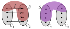
Figure 1: The way the vertex set $S^{\prime}$ intersects the vertex sets $C_{1}$ and $C_{2}$.

For the triplet $G,\ell,\mathcal{C}^{\prime}$, the sets in $M$ have all the same type and $|M|\geq 2^{k(q_{2}-1)}\cdot q_{1}+1$. Furthermore, the function $\phi^{\prime}$ has $q_{1}$ FO and $q_{2}-1$ MSO quantifiers. Therefore, by the inductive hypothesis we can remove a set from $M$ and the answer of the problem will not change, in other words we have that $G,\ell,\mathcal{C}^{\prime}\models\phi^{\prime}$ iff $G\setminus C_{1},\ell,\mathcal{C}^{\prime}_{1}\models\phi^{\prime}$, where $\mathcal{C}^{\prime}_{1}$ is the restriction of $\mathcal{C}^{\prime}$ on $V(G)\setminus C_{1}$. From the semantics of $\phi$ we have that $G\setminus C_{1},\ell,\mathcal{C}_{1}\models\phi.$

For the other direction, if $G\setminus C_{1},\ell,\mathcal{C}_{1}\models\phi$ then there exists $S_{1}\subseteq V(G)\setminus C_{1}$ such that $G\setminus C_{1},\ell,\mathcal{C}_{1}^{\prime}\models\phi[X_{i}\setminus D_{i}]$ with $\mathcal{C}_{1}(D_{i})\uparrow$ and $\mathcal{C}_{1}$ being a partial coloring function for which $\mathcal{C}_{1}^{\prime}(D_{i})=S_{1}$, and $\mathcal{C}_{1}^{\prime}$ agrees with $\mathcal{C}_{1}$ on all other values $D_{j}\neq D_{i}$.

As previously, $S_{1}$ partitions $C_{2},\ldots,C_{q^{\prime}}$ into $2^{k}$ equivalence classes, depending on the intersection of each set with $S_{1}$, such that sets placed in the same class (i.e. having isomorphic intersection with $S_{1}$) have the same type in $G\setminus C_{1},\ell,\mathcal{C}_{1}^{\prime}$. Hence, one of these classes has size at least $\frac{q^{\prime}-1}{2^{k}}=2^{k(q_{2}-1)}\cdot q_{1}$, call this class $M^{\prime}$. We construct a triplet $G,\ell,\mathcal{C}^{*}$ as follows: let $C_{j}\in M^{\prime}$ and $f^{\prime}$ be the isomorphism from $C_{j}$ to $C_{1}$; We set that $\mathcal{C}^{*}$ agrees with $\mathcal{C}$ on all sets except $D_{i}$; and for $D_{i}$ we have $\mathcal{C}^{*}(D_{i})=\mathcal{C}_{1}^{\prime}(D_{i})\cup f^{\prime}(S_{1}\cap C_{j})$. In other words, we define $\mathcal{C}^{*}$ in such a way that the set $C_{1}$ has the same type as all sets of the class $M^{\prime}$. But then we have $|M^{\prime}\cup\{C_{1}\}|\geq 2^{k(q_{2}-1)}\cdot q_{1}+1$ sets of the same type and by inductive hypothesis we have $G,\ell,\mathcal{C}^{*}\models\phi[X_{i}\setminus D_{i}]$. Therefore, by the semantics of MSO we have $G,\ell,\mathcal{C}\models\phi$.

Lemma 3.9.

For a triplet $G,\ell,\mathcal{C}$ with vertex integrity $\iota(G)\leq k$ and with $\ell,\mathcal{C}$ everywhere undefined and for a formula $\phi$ with $q_{1}$ FO quantifiers and $q_{2}$ MSO quantifiers, MSO Model Checking has a kernel of size $O(2^{(k^{2}+kq_{2})}\cdot q_{1}\cdot k)$, assuming we are given in the input $S\subseteq V(G)$ such that the largest component of $G\setminus S$ has size at most $k-|S|$.

Proof 3.10.

The proof is the same as for Lemma 3.5. The only thing that changes is the number of same-type components required to have before removing one such component ($q^{\prime}$ required by Lemma 3.7 versus $q+1$ required by Lemma 3.3).

Applying the straightforward algorithm for MSO Model-Checking that runs in $2^{q_{2}\cdot V(G)}\cdot V(G)^{q_{1}}\cdot poly|G|$ and Lemma 3.9 gives the complexity promised by Theorem 3.2.

4 Lower Bounds

In this section we show that the dependence of our meta-theorems on vertex integrity cannot be significantly improved, unless the ETH is false. Our strategy will be to present a unified construction which, starting from an arbitrary graph $G$ with $n$ vertices, produces a new graph $H(G)$, with small vertex integrity, such that we can deduce if two vertices of $G$ are connected using appropriate FO formulas that describe properties of $H$. This will, in principle, allow us to express an FO or MSO-expressible property of $G$ as a corresponding property of $H(G)$, and hence, if the original property is hard, to obtain a lower bound on model-checking on $H$. Let us describe this construction in more details.

Construction

We are given a graph $G$ on $n$ vertices, say $V(G)=\{v_{1},\ldots,v_{n}\}$, and $m$ edges. Let $k=\lceil\sqrt{\log n}\rceil$. We construct a graph $H$ as follows:

1. We begin constructing $V(H)$ by forming $n+m+1$ sets of vertices, called $S$, $W_{1},\ldots,W_{n}$, and $Y_{1},\ldots,Y_{m}$. We have $|S|=2k$, $|W_{i}|=k$ for all $i\in[n]$, and $|Y_{j}|=2k+1$ for all $j\in[m]$. The vertices of $S$ are numbered arbitrarily as $s_{1},s_{2},\ldots,s_{2k}$.

2. Internally, $S$ induces an independent set, each $W_{i}$, for $i\in[n]$ induces a clique, and each $Y_{j}$, for $j\in[m]$ induces a graph made up of two disjoint cliques of size $k$, denoted $Y_{j}^{1},Y_{j}^{2}$, and a vertex connected to all $2k$ vertices of the cliques $Y_{j}^{1},Y_{j}^{2}$.

3. For each $i\in[n]$, we attach a leaf to each vertex of $W_{i}$. For each $j\in[m]$, we attach two leaves to each vertex of $Y_{j}^{1}$, three leaves to each vertex of $Y_{j}^{2}$, and four leaves to the remaining vertex of $Y_{j}$.

4. For each $i\in[n]$, number the vertices of $W_{i}$ arbitrarily as $w_{(i,1)},w_{(i,2)},\ldots,w_{(i,k)}$. For each $\beta\in[k]$ we connect $w_{(i,\beta)}$ to $s_{\beta}$. Furthermore, let $b_{1}b_{2}\ldots b_{k^{2}}$ be the binary representation of $i-1$ with the least significant digit first, that is, a sequence of bits such that $\sum_{\beta}b_{\beta}2^{\beta-1}=i-1$. Note that $k^{2}\geq\log n$, therefore $k^{2}$ bits are sufficient to represent all numbers from $0$ to $n-1$. We partition this binary representation into $k$ blocks of $k$ bits. For $\beta\in[k]$ we consider the bits $b_{(\beta-1)k+1}\ldots b_{\beta k}$ and we use these bits to determine the connections between $w_{(i,\beta)}$ and the vertices $s_{k+1},\ldots,s_{2k}$. More precisely, for $\beta,\gamma\in[k]$, we set that $w_{(i,\beta)}$ is connected to $s_{k+\gamma}$ if and only if $b_{(\beta-1)k+\gamma}$ is equal to $1$.

5. For each $j\in[m]$ we do the following. Suppose the $j$-th edge of $G$ has endpoints $v_{i_{1}},v_{i_{2}}$. We number the vertices of $Y_{j}^{1}$ as $y_{(j,1)}^{1},\ldots,y_{(j,k)}^{1}$, and the vertices of $Y_{j}^{2}$ as $y_{(j,1)}^{2},\ldots,y_{(j,k)}^{2}$ in some arbitrary way. Now for all $\beta\in[k]$ we set that $y_{(j,\beta)}^{1}$ has the same neighbors in $S$ as $w_{(i_{1},\beta)}$ and $y_{(j,\beta)}^{2}$ has the same neighbors in $S$ as $w_{(i_{2},\beta)}$.

The construction of our graph is now complete. The intuition behind this construction is that each clique $W_{i}$ represents a vertex $v_{i}\in V(G)$. In order to distinguish the vertices, we use the $k^{2}\geq\log n$ possible edges between vertices in $W_{i}$ and the second part of $S$, that is $\{s_{k+1},\ldots,s_{2k}\}$. These edges should represent the binary representation of $i$. See Figure 2 for an example.

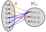
Figure 2: The connection between $S$ and the set $W_{47}$. For this example $k=3$, we can represent up to $2^{9}$ numbers in binary. In order to represent $47_{10}=000101111_{2}$, we shall connect $w_{(47,1)}$ with $s_{4},s_{5}$ and $s_{6}$ in order to represent the three least significant bits (which are all 1), and $w_{(47,2)}$ with $s_{4}$ and $s_{6}$ to represent the next triad of bits. The three most significant bits are all 0, therefore $w_{(47,3)}$ is not connected to any of $s_{4},s_{5},s_{6}$.

Vertices of $H$ may be (arbitrarily) labeled for the purpose of the construction but for the purpose of Model-Checking the graph $H$ is unlabeled. In order to give a numbering to the vertices of $W_{i}$, we use the matching between $W_{i}$ and the first $k$ vertices of the set $S$ (the first vertex of $W_{i}$ connects to the first vertex of $S$, etc).

The sets $Y_{j}$ represent edges in $G$. If the $j^{\textrm{th}}$ edge in $E(G)$ is the edge $(v_{i_{1}}v_{i_{2}})$, then $Y_{j}^{1}$ should have the same connections with $S$ as the set $W_{i_{1}}$ (similarly $Y_{j}^{2}$, $W_{i_{2}}$). In order to check in $H$ whether $(v_{i_{1}},v_{i_{2}})$ is an edge, we shall check if there exists a set $Y_{j}$ such that each vertex of $Y_{j}^{1}$ has the same neighborhood in $S$ as a vertex of $W_{i_{1}}$ and each vertex of $Y_{j}^{2}$ has the same neighborhood in $S$ as a vertex of $W_{i_{2}}$.

It is crucial here that the construction is such that $W_{i},W_{i^{\prime}}$ are distinguishable for $i\neq i^{\prime}$ in terms of their neighborhoods in $S$, that is, there always exists $w\in W_{i}$ for which no $w^{\prime}\in W_{i^{\prime}}$ has $N(w)\cap S=N(w^{\prime})\cap S$. We will show that it is not hard to express this property in FO logic. Furthermore, the leaves we have attached to various vertices will allow us to distinguish in FO logic whether a vertex belongs in a set $W_{i}$, $Y_{j}^{1}$, or $Y_{j}^{2}$.

We now establish some basic properties about $H$ and what can be expressed about its vertices in FO logic:

Lemma 4.1.

There exist FO formulas $\phi_{W}(x_{1}),\phi_{Y1}(x_{1}),\phi_{Y2}(x_{1}),\phi_{S}(x_{1})$ using one free variable $x_{1}$ and FO formulas $\phi_{WY}(x_{1},x_{2}),\phi_{adj}(x_{1},x_{2})$ using two free variables $x_{1},x_{2}$, such that any graph $H$ constructed as described above satisfies the following properties, for any coloring function $\mathcal{C}$.

1. We have $\iota(H)=O(\sqrt{\log n})$ and $|V(H)|=O(n^{2}\sqrt{\log n})$.

2. For each $i,i^{\prime}\in[n]$ with $i\neq i^{\prime}$, there exists a vertex $w\in W_{i}$ such that for all $w^{\prime}\in W_{i^{\prime}}$ we have $N(w)\cap S\neq N(w^{\prime})\cap S$.

3. $H,\ell,\mathcal{C}\models\phi_{W}[x_{1}\setminus u_{1}]$ (respectively $H,\ell,\mathcal{C}\models\phi_{Y1}[x_{1}\setminus u_{1}]$, $H,\ell,\mathcal{C}\models\phi_{Y2}[x_{1}\setminus u_{1}]$, $H,\ell,\mathcal{C}\models\phi_{S}[x_{1}\setminus u_{1}]$) if and only if $\ell(u_{1})\in W_{i}$ for some $i\in[n]$ (respectively $\ell(u_{1})\in Y_{j}^{1}$, $\ell(u_{1})\in Y_{j}^{2}$, for some $j\in[m]$, $\ell(u_{1})\in S$).

4. $H,\ell,\mathcal{C}\models\phi_{WY}[x_{1}\setminus u_{1}][x_{2}\setminus u_{2}]$ if and only if $\ell(u_{1})\in W_{i}$ for some $i\in[n]$, $\ell(u_{2})\in Y_{j}^{\alpha}$ for some $j\in[m],\alpha\in\{1,2\}$, and for all $\beta\in[k]$ we have $N(w_{(i,\beta)})\cap S=N(y_{(j,\beta)}^{\alpha})\cap S$.

5. $H,\ell,\mathcal{C}\models\phi_{adj}[x_{1}\setminus u_{1}][x_{2}\setminus u_{2}]$ if and only if $\ell(u_{1})\in W_{i}$ and $\ell(u_{2})\in W_{i^{\prime}}$ for some $i,i^{\prime}\in[n]$ such that $(v_{i},v_{i^{\prime}})\in E(G)$.

Proof 4.2.

For the first property, we observe that the largest component of $H\setminus S$ has size at most $10\sqrt{\log n}+2$, while $|S|\leq 2\sqrt{\log n}+2$. Furthermore, we have at most $m+n=O(n^{2})$ components after removing $S$.

For the second property, since $i\neq i^{\prime}$, their binary representations differ in some bit. Let $\beta,\gamma\in[k]$ be such that if $b_{1}\ldots b_{k^{2}}$ is the binary representation of $i-1$ and $b_{1}^{\prime}\ldots b_{k^{2}}^{\prime}$ is the binary representation of $i^{\prime}-1$, we have $b_{(\beta-1)k+\gamma}\neq b^{\prime}_{(\beta-1)k+\gamma}$. But then, exactly one of $w_{(i,\beta)},w_{(i^{\prime},\beta)}$ is connected to $s_{k+\gamma}$. Furthermore, $w_{(i,\beta)}$ is connected to $s_{\beta}$, but the only neighbor of $s_{\beta}$ in $W_{i^{\prime}}$ is $w_{(i^{\prime},\beta)}$. Hence, $w_{(i,\beta)}$ is the claimed vertex.

For the third property, observe that, in $H$, vertices of $S$ have no leaves attached, vertices of each $X_{i}$ have one leaf attached, vertices of $Y_{j}^{1}$ have two leaves attached, vertices of $Y_{j}^{2}$ have three leaves attached, and the remaining vertices have four leaves attached. Hence, it suffices to be able to express in FO the property “$x_{1}$ has exactly $c$ leaves attached”, where $c\in\{0,1,2,3\}$. This is not hard to do. For example, the formula $\phi_{2}(x_{1}):=\exists x_{2}\exists x_{3}\forall x_{4}\left((x_{2}\sim x_{1})\land(x_{3}\sim x_{1})\land(x_{2}\neq x_{3})\land\left((x_{4}=x_{1})\lor\left(\neg(x_{4}\sim x_{2})\land\neg(x_{4}\sim x_{3})\right)\right)\right)$ expresses the property that $x_{1}$ has at least two leaves attached to it. Using the same ideas we can construct $\phi_{c}(x_{1})$, for $c\in\{1,2,3,4\}$ and then $\phi_{S}(x_{1}):=\neg\phi_{1}(x_{1})$, $\phi_{W}(x_{1}):=\phi_{1}(x_{1})\land\neg\phi_{2}(x_{1})$, $\phi_{Y1}:=\phi_{2}(x_{1})\land\neg\phi_{3}(x_{1})$, $\phi_{Y2}(x_{1}):=\phi_{3}(x_{1})\land\neg\phi_{4}(x_{1})$.

For the fourth property, we set $\phi_{WY}(x_{1},x_{2}):=\phi_{WY1}(x_{1},x_{2})\lor\phi_{WY2}(x_{1},x_{2})$, where we define two formulas $\phi_{WY\alpha}$ depending on whether $\alpha=1$ or $\alpha=2$. We have

$$\phi_{WY\alpha}(x_{1},x_{2}) := \phi_{W}(x_{1})\land\phi_{Y\alpha}(x_{2})\land\forall x_{3}\big{(}(\neg\phi_{W}(x_{3}))\lor(\neg(x_{3}\sim x_{1})\land\neg(x_{3}=x_{1}))\lor$$

$$\exists x_{4}\left(\phi_{Y1}(x_{4})\land(x_{4}\sim x_{2}\lor x_{4}=x_{2})\land\forall x_{5}\left(\phi_{S}(x_{5})\to(x_{5}\sim x_{3}\leftrightarrow x_{5}\sim x_{4})\right)\right)\big{)}$$

What we are saying here is that $\phi_{WY1}[x_{1}\setminus u_{1}][x_{2}\setminus u_{2}]$ is satisfied if $\ell(u_{1})\in W_{i},\ell(u_{2})\in Y_{j}^{1}$, for some $i\in[n],j\in[m]$, and for every $x_{3}\in W_{i}$ there exists $x_{4}\in Y_{j}^{1}$ such that $N(x_{3})\cap S=N(x_{4})\cap S$. Therefore, if this property holds, then $W_{i}$ and $Y_{j}^{1}$ represent the same vertex of $V$ (similarly for $\phi_{WY2}$).

For the last property, we set

$$\phi_{adj}(x_{1},x_{2}) := \phi_{W}(x_{1})\land\phi_{W}(x_{2})\land\exists x_{3}\exists x_{4}\big{(}(\phi_{Y1}(x_{3})\land\phi_{Y_{2}}(x_{4}))\lor(\phi_{Y1}(x_{4})\land\phi_{Y_{2}}(x_{3}))\big{)}\land$$

$$\phi_{WY}(x_{1},x_{3})\land\phi_{WY}(x_{2},x_{4})\land\exists x_{5}(\neg\phi_{S}(x_{5})\land x_{3}\sim x_{5}\land x_{4}\sim x_{5})$$

In other words, $H,\ell,\mathcal{C}\models\phi_{adj}[x_{1}\setminus u_{1}][x_{2}\setminus u_{2}]$ if (i) $\ell(u_{1})\in W_{i}$ and $\ell(u_{2})\in W_{i^{\prime}}$, for some $i,i^{\prime}\in[n]$ (ii) there exist $x_{3},x_{4}$ such that $x_{3}\in Y_{j}^{1}$ and $x_{4}\in Y_{j}^{2}$ for the same $j$; this is verified because $x_{3},x_{4}$ have a common neighbor $x_{5}$ that does not belong in $S$ (iii) $W_{i},W_{i^{\prime}}$ correspond to the same pair of vertices as the set $Y_{j}=Y_{j}^{1}\cup Y_{j}^{2}$, which means that $(v_{i},v_{i^{\prime}})\in E(G)$.

We are now ready to prove our lower bounds.

Theorem 4.3.

If there exists an algorithm which, given an FO formula $\phi$ with $q$ quantifiers, an integer $k$, and a graph $G$ on $n$ vertices with $\iota(G)=k$, decides whether $G\models\phi$ in time $2^{o(k^{2}q)}n^{O(1)}$, then the ETH is false.

Proof 4.4.

We perform a reduction from $q$-Clique. It is well-known that, given a graph $G$ on $n$ vertices it is not possible to decide if $G$ contains a clique of size $q$ in time $n^{o(q)}$, unless the ETH is false [8]. We claim that we construct the graph $H(G)$, as previously described, and an FO formula $\phi_{C}$ such that $\phi_{C}$ will contain $O(q)$ quantifiers and $H,\ell,\mathcal{C}\models\phi_{C}$ for the nowhere defined functions $\ell,\mathcal{C}$ if and only if $G$ has a $q$-clique. If we achieve this, then, since by Lemma 4.1 we have $k=O(\sqrt{\log n})$, and the size of $H$ is polynomially related to the size of $G$, the stated running time would become $2^{o(q(\sqrt{\log n})^{2})}n^{O(1)}=n^{o(q)}$ and we refute the ETH. Our goal is then to define such an FO formula $\phi_{C}$. We define

$$\phi_{C} := \exists x_{1}\exists x_{2}\ldots\exists x_{q}\bigwedge_{i\in[q]}\phi_{W}(x_{i})\land\bigwedge_{i,i^{\prime}\in[q],i\neq i^{\prime}}(x_{i}\neq x_{i^{\prime}})$$

$$\forall x_{q+1}\forall x_{q+2}\bigwedge_{i\in[q]}\big{(}\neg(x_{q+1}=x_{i})\big{)}\lor\bigwedge_{i\in[q]}\big{(}\neg(x_{q+2}=x_{i})\big{)}\lor(x_{q+1}=x_{q+2})\lor$$

$$\phi_{adj}(x_{q+1},x_{q+2})$$

We now claim that by the construction of $H$, we have that $H,\ell,\mathcal{C}\models\phi_{C}$ if and only if $G$ has a clique. If $G$ has a clique $\{v_{i_{1}},v_{i_{2}},\ldots,v_{i_{q}}\}$, we map $x_{1},x_{2},\ldots,x_{q}$ to arbitrary vertices of $W_{i_{1}},\ldots,W_{i_{q}}$. For the next part of the formula, either $x_{q+1},x_{q+2}$ correspond to some (different) $x_{i},x_{i^{\prime}}$ or the formula is true. Last, we claim that $H,\ell^{\prime},\mathcal{C}\models\phi_{adj}[x_{q+1}\setminus u_{i}][x_{q+2}]\setminus u_{i^{\prime}}]$, where $x_{i},x_{i^{\prime}}$ are substituted by $u_{i},u_{i^{\prime}}$ and $\ell^{\prime}(u_{i})\in W_{i},\ell^{\prime}(u_{i^{\prime}})\in W_{i^{\prime}}$. Indeed, because we have a clique in $G$, by construction there exists a $Y_{j}$ such that each vertex of $Y_{j}^{1}$ has the same neighborhood in $S$ as $W_{i}$ and each vertex of $Y_{j}^{2}$ has the same neighborhood in $S$ as $W_{i^{\prime}}$ (or the same with the roles of $Y_{j}^{1},Y_{j}^{2}$ reversed). Hence, $\phi_{adj}$ is satisfied.

For the converse direction, suppose that $H,\ell,\mathcal{C}\models\phi_{C}$ for the nowhere defined labeling function $\ell$. Then there exists a labeling function $\ell^{\prime}$ that assigns $\ell^{\prime}(u_{1}),\ell^{\prime}(u_{2}),\ldots,\ell^{\prime}(u_{q})$ to some vertices of $\bigcup_{i\in[n]}W_{i}$ and is undefined everywhere else such that $\ell^{\prime}(u_{i})\neq\ell^{\prime}(u_{i^{\prime}})$ for $i\neq i^{\prime}$ and $H,\ell^{\prime},\mathcal{C}\models\phi_{C^{\prime}}$ where

$$\phi_{C^{\prime}}:=\forall x_{q+1}\forall x_{q+2}\bigwedge_{i\in[q]}\big{(}\neg(x_{q+1}=u_{i})\big{)}\lor\bigwedge_{i\in[q]}\big{(}\neg(x_{q+2}=u_{i})\big{)}\lor(x_{q+1}=x_{q+2})\lor\phi_{adj}(x_{q+1},x_{q+2})$$

We extract a multi-set $S$ of $q$ vertices of $G$ as follows: for $\beta\in[q]$, if $\ell^{\prime}(u_{\beta})\in W_{i}$, then we add $v_{i}$ to $S$. We claim that for any two elements $v_{i},v_{i^{\prime}}$ of $S$ we have $(v_{i},v_{i^{\prime}})\in E$. If we prove this, then the vertices of $S$ are distinct and form a $q$-clique in $G$.

Since we have universal quantifications for $x_{q+1},x_{q+2}$, we can define a new labeling function $\ell^{\prime\prime}$, with $\ell^{\prime\prime}(u_{q+1})=\ell^{\prime}(u_{i})$ and $\ell^{\prime\prime}(u_{q+2})=\ell^{\prime}(u_{i^{\prime}})$, for any $i,i^{\prime}\in[q],i\neq i^{\prime}$, with $\ell^{\prime\prime},\ell^{\prime}$ agreeing everywhere else. Observe that this selection imposes that $H,\ell^{\prime\prime},\mathcal{C}\models\phi_{adj}[x_{q+1}\setminus u_{i}][x_{q+2}\setminus u_{i^{\prime}}]$ and from property 5 of Lemma 4.1 we get that $\ell^{\prime}(u_{i}),\ell^{\prime}(u_{i^{\prime}})$ belong to two different $W_{j},W_{j^{\prime}}$ that correspond to the endpoints of an edge of $G$.

Theorem 4.5.

There is an MSO formula $\phi$ such that we have the following: if there exists an algorithm which, given a graph $G$ with $n$ vertices and $\iota(G)=k$, decides whether $G\models\phi$ in time $2^{2^{o(k^{2})}}n^{O(1)}$, then the ETH is false.

Proof 4.6.

Our strategy is similar to that of Theorem 4.3, except that we will now reduce from 3-Coloring, which is known not to be solvable in $2^{o(n)}$ on graphs on $n$ vertices, under the ETH [33]. We will produce a formula $\phi_{Col}$ with the property that $H,\ell,\mathcal{C}\models\phi_{Col}$ for the nowhere defined functions $\ell,\mathcal{C}$ if and only if $G$ is 3-colorable. Since $k=O(\sqrt{\log n})$ an algorithm running in $2^{2^{o(k^{2})}}$ would imply a $2^{o(n)}$ algorithm for 3-coloring $G$, contradicting the ETH. We define

$$\phi_{Col} := \exists X_{1}\exists X_{2}\exists X_{3}\forall x_{1}\forall x_{2}(x_{1}\in X_{1}\lor x_{1}\in X_{2}\lor x_{1}\in X_{3})\land$$

$$\bigwedge_{i=1,2,3}\phi_{adj}(x_{1},x_{2})\to\big{(}x_{1}\in X_{i}\to\neg(x_{2}\in X_{i})\big{)}$$

Assume that $G$ has a proper 3-coloring $c:V\to[3]$. Then we define, for $\alpha\in[2]$ $S_{\alpha}=\bigcup_{i:c(v_{i})=\alpha}W_{i}$ and $S_{3}=V(H)\setminus(S_{1}\cup S_{2})$. Let $\mathcal{C}^{\prime}$ be a coloring function such that $\mathcal{C}^{\prime}(D_{\alpha})=S_{\alpha}$ for $\alpha=1,2,3$ and $\mathcal{C}^{\prime}(D_{\alpha^{\prime}})\uparrow$ for $\alpha^{\prime}\not\in[3]$. We claim that $H,\ell,\mathcal{C}^{\prime}\models\phi_{Col}[X_{1}\setminus D_{1}][X_{2}\setminus D_{2}][X_{3}\setminus D_{3}]$. Indeed, for any labeling function $\ell^{\prime}$ that defines only $\ell^{\prime}(u_{1})$ and $\ell^{\prime}(u_{2})$ we have (i) $H,\ell^{\prime},\mathcal{C}^{\prime}\models u_{1}\in D_{1}\lor u_{1}\in D_{2}\lor u_{1}\in D_{3}$ (since $\mathcal{C}^{\prime}(D_{1}),\mathcal{C}^{\prime}(D_{2}),\mathcal{C}^{\prime}(D_{3})$ is a partition of $V(H)$); (ii) If $H,\ell^{\prime},\mathcal{C}^{\prime}\models\phi_{adj}[x_{1}\setminus u_{1}][x_{2}\setminus u_{2}]$ then $\ell^{\prime}(u_{1})\in W_{i},\ell^{\prime}(u_{2})\in W_{i^{\prime}}$ for some $i,i^{\prime}\in[n],i\neq i^{\prime}$ with $(v_{i},v_{i^{\prime}})\in E(G)$ (from property 5 of Lemma 4.1). Therefore $c(v_{i})\neq c(v_{i^{\prime}})$ so for $\alpha\in[3]$ $H,\ell^{\prime},\mathcal{C}^{\prime}\models\left(u_{1}\in D_{\alpha}\to\neg(u_{2}\in D_{\alpha})\right)$.

For the converse direction, suppose that $H,\ell,\mathcal{C}\models\phi_{Col}$ for the nowhere defined $\ell,\mathcal{C}$. Then there exists a coloring function $\mathcal{C}^{\prime}$ such that $\mathcal{C}^{\prime}(D_{\alpha})=S_{\alpha}$, for $\alpha\in[3]$ and $H,\ell,\mathcal{C}^{\prime}\models\phi_{Col}[X_{1}\setminus D_{1}][X_{2}\setminus D_{2}][X_{3}\setminus D_{3}]$. We extract a coloring of $V(G)$ as follows: for $i\in[n]$ we set $c(v_{i})$ to be the minimum $\alpha$ such that $W_{i}\cap S_{\alpha}\neq\emptyset$. We show that the coloring $c:V(G)\to[3]$ defined in this way is proper. Consider $i,i^{\prime}\in[n]$ such that $(v_{i},v_{i^{\prime}})\in E(G)$. Let $\ell^{\prime}$ be a labeling function such that $\ell^{\prime}(u_{1})\in W_{i}\cap S_{c(v_{i})}$ and $\ell^{\prime}(u_{2})\in W_{i^{\prime}}\cap S_{c(v_{i^{\prime}})}$. Observe that $W_{i}\cap S_{c(v_{i})}\neq\emptyset$ by the definition of $c(v_{i})$. Then $H,\ell^{\prime},\mathcal{C}^{\prime}\models\phi_{adj}[x_{1}\setminus u_{1}][x_{2}\setminus u_{2}]$. Therefore we have that for $\alpha\in[3]$, $H,\ell^{\prime},\mathcal{C}^{\prime}\models\left(u_{1}\in D_{\alpha}\to\neg(u_{2}\in D_{\alpha})\right)$. Therefore $S_{c(v_{i})}\neq S_{c(v_{i^{\prime}})}$, which means that $c(v_{i})\neq c(v_{i^{\prime}})$.

5 Conclusions

We have given tight upper and lower bounds on the complexity of model checking first-order and monadic second-order logic formulas parameterized by the vertex integrity of the input graph. Our results are of course only of theoretical interest, as the algorithms of Theorem 3.1 and Theorem 3.2 are not meant to be implemented in practice. One interesting avenue for further research would be to extend our results to monadic second-order logic with edge-set quantifiers, also known as MSO₂ logic. In the case of meta-theorems for vertex cover, the extension from MSO₁ to MSO₂ is not too complicated, as in a graph with vertex cover $k$, every set of edges can be described as the union of $k$ sets of vertices (every edge is incident on a vertex of the vertex cover, so it suffices to give, for each such vertex, the set of second endpoints of the edges selected incident to this vertex). It would be interesting to see if this basic argument can be extended to vertex integrity, and whether this makes the complexity of model checking MSO₂ formulas significantly worse than the complexity we gave for MSO₁ formulas.

References

- [1] Rémy Belmonte, Eun Jung Kim, Michael Lampis, Valia Mitsou, and Yota Otachi. Grundy distinguishes treewidth from pathwidth. SIAM J. Discret. Math., 36(3):1761–1787, 2022.
- [2] Rémy Belmonte, Michael Lampis, and Valia Mitsou. Parameterized (approximate) defective coloring. SIAM J. Discret. Math., 34(2):1084–1106, 2020.
- [3] Hans L. Bodlaender, Fedor V. Fomin, Daniel Lokshtanov, Eelko Penninkx, Saket Saurabh, and Dimitrios M. Thilikos. (Meta) kernelization. J. ACM, 63(5):44:1–44:69, 2016.
- [4] Hans L. Bodlaender, Tesshu Hanaka, Yasuaki Kobayashi, Yusuke Kobayashi, Yoshio Okamoto, Yota Otachi, and Tom C. van der Zanden. Subgraph isomorphism on graph classes that exclude a substructure. Algorithmica, 82(12):3566–3587, 2020.
- [5] Édouard Bonnet, Eun Jung Kim, Stéphan Thomassé, and Rémi Watrigant. Twin-width I: tractable FO model checking. In FOCS, pages 601–612. IEEE, 2020.
- [6] Bruno Courcelle. The monadic second-order logic of graphs. I. recognizable sets of finite graphs. Inf. Comput., 85(1):12–75, 1990.
- [7] Bruno Courcelle, Johann A. Makowsky, and Udi Rotics. Linear time solvable optimization problems on graphs of bounded clique-width. Theory Comput. Syst., 33(2):125–150, 2000.
- [8] Marek Cygan, Fedor V. Fomin, Lukasz Kowalik, Daniel Lokshtanov, Dániel Marx, Marcin Pilipczuk, Michal Pilipczuk, and Saket Saurabh. Parameterized Algorithms. Springer, 2015.
- [9] Anuj Dawar, Martin Grohe, Stephan Kreutzer, and Nicole Schweikardt. Approximation schemes for first-order definable optimisation problems. In LICS, pages 411–420. IEEE Computer Society, 2006.
- [10] Holger Dell, Eun Jung Kim, Michael Lampis, Valia Mitsou, and Tobias Mömke. Complexity and approximability of parameterized max-csps. Algorithmica, 79(1):230–250, 2017.
- [11] Pål Grønås Drange, Markus S. Dregi, and Pim van ’t Hof. On the computational complexity of vertex integrity and component order connectivity. Algorithmica, 76(4):1181–1202, 2016.
- [12] Pavel Dvorák, Eduard Eiben, Robert Ganian, Dusan Knop, and Sebastian Ordyniak. Solving integer linear programs with a small number of global variables and constraints. In Carles Sierra, editor, Proceedings of the Twenty-Sixth International Joint Conference on Artificial Intelligence, IJCAI 2017, Melbourne, Australia, August 19-25, 2017, pages 607–613. ijcai.org, 2017. doi:10.24963/ijcai.2017/85.
- [13] Pavel Dvořák and Dusan Knop. Parameterized complexity of length-bounded cuts and multicuts. Algorithmica, 80(12):3597–3617, 2018.
- [14] Zdenek Dvořák, Daniel Král, and Robin Thomas. Testing first-order properties for subclasses of sparse graphs. J. ACM, 60(5):36:1–36:24, 2013.
- [15] Eduard Eiben, Robert Ganian, and Stefan Szeider. Meta-kernelization using well-structured modulators. Discret. Appl. Math., 248:153–167, 2018.
- [16] Michael R. Fellows, Fedor V. Fomin, Daniel Lokshtanov, Frances A. Rosamond, Saket Saurabh, Stefan Szeider, and Carsten Thomassen. On the complexity of some colorful problems parameterized by treewidth. Inf. Comput., 209(2):143–153, 2011. doi:10.1016/j.ic.2010.11.026.
- [17] Jirí Fiala, Petr A. Golovach, and Jan Kratochvíl. Parameterized complexity of coloring problems: Treewidth versus vertex cover. Theor. Comput. Sci., 412(23):2513–2523, 2011. doi:10.1016/j.tcs.2010.10.043.
- [18] Markus Frick. Generalized model-checking over locally tree-decomposable classes. Theory Comput. Syst., 37(1):157–191, 2004.
- [19] Markus Frick and Martin Grohe. Deciding first-order properties of locally tree-decomposable structures. J. ACM, 48(6):1184–1206, 2001.
- [20] Markus Frick and Martin Grohe. The complexity of first-order and monadic second-order logic revisited. Ann. Pure Appl. Log., 130(1-3):3–31, 2004.
- [21] Jakub Gajarský and Petr Hliněný. Kernelizing MSO properties of trees of fixed height, and some consequences. Log. Methods Comput. Sci., 11(1), 2015.
- [22] Robert Ganian. Improving vertex cover as a graph parameter. Discret. Math. Theor. Comput. Sci., 17(2):77–100, 2015.
- [23] Robert Ganian, Petr Hliněný, Jaroslav Nešetřil, Jan Obdržálek, and Patrice Ossona de Mendez. Shrub-depth: Capturing height of dense graphs. Log. Methods Comput. Sci., 15(1), 2019.
- [24] Robert Ganian, Petr Hliněný, Jaroslav Nešetřil, Jan Obdržálek, Patrice Ossona de Mendez, and Reshma Ramadurai. When trees grow low: Shrubs and fast MSO1. In MFCS, volume 7464 of Lecture Notes in Computer Science, pages 419–430. Springer, 2012.
- [25] Robert Ganian, Fabian Klute, and Sebastian Ordyniak. On structural parameterizations of the bounded-degree vertex deletion problem. Algorithmica, 83(1):297–336, 2021.
- [26] Robert Ganian and Jan Obdržálek. Expanding the expressive power of monadic second-order logic on restricted graph classes. In IWOCA, volume 8288 of Lecture Notes in Computer Science, pages 164–177. Springer, 2013.
- [27] Robert Ganian, Sebastian Ordyniak, and M. S. Ramanujan. On structural parameterizations of the edge disjoint paths problem. Algorithmica, 83(6):1605–1637, 2021. doi:10.1007/s00453-020-00795-3.
- [28] Robert Ganian, Friedrich Slivovsky, and Stefan Szeider. Meta-kernelization with structural parameters. J. Comput. Syst. Sci., 82(2):333–346, 2016.
- [29] Tatsuya Gima, Tesshu Hanaka, Masashi Kiyomi, Yasuaki Kobayashi, and Yota Otachi. Exploring the gap between treedepth and vertex cover through vertex integrity. In CIAC, volume 12701 of Lecture Notes in Computer Science, pages 271–285. Springer, 2021.
- [30] Martin Grohe and Stephan Kreutzer. Methods for algorithmic meta theorems. Model Theoretic Methods in Finite Combinatorics, 558:181–206, 2011.
- [31] Gregory Z. Gutin, Mark Jones, and Magnus Wahlström. The mixed chinese postman problem parameterized by pathwidth and treedepth. SIAM J. Discrete Math., 30(4):2177–2205, 2016. doi:10.1137/15M1034337.
- [32] Ararat Harutyunyan, Michael Lampis, and Nikolaos Melissinos. Digraph coloring and distance to acyclicity. In STACS, volume 187 of LIPIcs, pages 41:1–41:15. Schloss Dagstuhl - Leibniz-Zentrum für Informatik, 2021.
- [33] Russell Impagliazzo, Ramamohan Paturi, and Francis Zane. Which problems have strongly exponential complexity? J. Comput. Syst. Sci., 63(4):512–530, 2001. doi:10.1006/jcss.2001.1774.
- [34] Ioannis Katsikarelis, Michael Lampis, and Vangelis Th. Paschos. Structural parameters, tight bounds, and approximation for (k, r)-center. Discret. Appl. Math., 264:90–117, 2019.
- [35] Ioannis Katsikarelis, Michael Lampis, and Vangelis Th. Paschos. Structurally parameterized -scattered set. Discrete Applied Mathematics, 2020. doi:https://doi.org/10.1016/j.dam.2020.03.052.
- [36] Leon Kellerhals and Tomohiro Koana. Parameterized complexity of geodetic set. In IPEC, volume 180 of LIPIcs, pages 20:1–20:14. Schloss Dagstuhl - Leibniz-Zentrum für Informatik, 2020.
- [37] Dusan Knop, Martin Koutecký, Tomás Masarík, and Tomás Toufar. Simplified algorithmic metatheorems beyond MSO: treewidth and neighborhood diversity. Log. Methods Comput. Sci., 15(4), 2019.
- [38] Dusan Knop, Tomás Masarík, and Tomás Toufar. Parameterized complexity of fair vertex evaluation problems. In MFCS, volume 138 of LIPIcs, pages 33:1–33:16. Schloss Dagstuhl - Leibniz-Zentrum für Informatik, 2019.
- [39] Michael Lampis. Algorithmic meta-theorems for restrictions of treewidth. Algorithmica, 64(1):19–37, 2012. doi:10.1007/s00453-011-9554-x.
- [40] Michael Lampis. Model checking lower bounds for simple graphs. Log. Methods Comput. Sci., 10(1), 2014.
- [41] Michael Lampis. Minimum stable cut and treewidth. In ICALP, volume 198 of LIPIcs, pages 92:1–92:16. Schloss Dagstuhl - Leibniz-Zentrum für Informatik, 2021.
- [42] Michael Lampis and Valia Mitsou. Treewidth with a quantifier alternation revisited. In IPEC, volume 89 of LIPIcs, pages 26:1–26:12. Schloss Dagstuhl - Leibniz-Zentrum für Informatik, 2017.
- [43] Michal Pilipczuk. Problems parameterized by treewidth tractable in single exponential time: A logical approach. In MFCS, volume 6907 of Lecture Notes in Computer Science, pages 520–531. Springer, 2011.
- [44] Stefan Szeider. Monadic second order logic on graphs with local cardinality constraints. ACM Trans. Comput. Log., 12(2):12:1–12:21, 2011.