Structure and Pore Size Distribution in Nanoporous Carbon

Abstract

We study the structural and mechanical properties of nanoporous (NP) carbon materials by extensive atomistic machine-learning (ML) driven molecular dynamics (MD) simulations. To this end, we retrain a ML Gaussian approximation potential (GAP) for carbon by recalculating the a-C structural database of Deringer and Csányi adding van der Waals interactions. Our GAP enables a notable speedup and improves the accuracy of energy and force predictions. We use the GAP to thoroughly study the atomistic structure and pore-size distribution in computational NP carbon samples. These samples are generated by a melt-graphitization-quench MD procedure over a wide range of densities (from 0.5 to 1.7 g/cm³) with structures containing 131,072 atoms. Our results are in good agreement with experimental data for the available observables, and provide a comprehensive account of structural (radial and angular distribution functions, motif and ring counts, X-ray diffraction patterns, pore characterization) and mechanical (elastic moduli and their evolution with density) properties. Our results show relatively narrow pore-size distributions, where the peak position and width of the distributions are dictated by the mass density of the materials. Our data allow further work on computational characterization of NP carbon materials, in particular for energy-storage applications, as well as suggest future experimental characterization of NP carbon-based materials.

Department of Applied Physics, QTF Center of Excellence, Aalto University, FIN-00076 Aalto, Espoo, Finland College of Physical Science and Technology, Bohai University, Jinzhou, 121013, China Interdisciplinary Centre for Mathematical Modelling and Department of Mathematical Sciences, Loughborough University, Loughborough, Leicestershire LE11 3TU, United Kingdom

1 Introduction

Nanoporous materials, where the pore-size distribution can be tuned according to growth conditions, can be engineered for specific applications, such as ionic and molecular transport ¹, biosensors ², air and water purification ³, or energy storage ⁴. In particular, nanopores in disordered graphitic carbons arise due to the misalignment and local curvature of the graphene-like sheets that make up these materials. These pores are defined as any interstitial space between graphene planes larger than the typical interlayer spacing in graphite ($\approx$ 3.5 Å) ⁴. When the pore sizes are of the order of a few nanometers, the graphitic carbons are referred to as “nanoporous” (NP) carbons. Nanopores significantly increase the effective surface area of NP carbons and confers this class of carbon materials with the ability to intercalate a number of small particles ⁵. Most notably, the nanopores can accommodate ions which can then migrate through the material or intercalate/deintercalate upon application of an external electric field, a mechanism exploited, for instance, in Li-ion batteries ⁴.

In addition to the existence and utility of pores in NP carbons, graphitic carbons in general display many attractive features that make them versatile materials for a number of technological and industrial applications. They are chemically stable, thanks to the large cohesive energy of the $sp^{2}$ bonds in elemental carbon. This makes them naturally resistant to corrosion and other degradation processes affecting material lifetimes in devices where electrochemical reactions are taking place, such as electrochemical sensors and batteries ^{2, 4}. Graphitic carbons also display some astonishing mechanical, thermal and electronic properties, with graphene or carbon nanotubes (CNTs) topping the charts of known materials in terms of some of their physical properties ^{6, 7, 8}. At the same time, carbon materials can be chemically functionalized to alter their reactivity, an important example being graphene oxide (GO) ^{9, 10}.

While graphite itself shows formidable in-plane strength, it can be easily deformed along the direction of stacking of its constituent graphene monolayers. On the other hand, disordered graphitic carbons, such as NP and glassy carbons (GCs), can show isotropic mechanical response to dimensional changes in all spatial directions even in the absence of noticeable $sp^{3}$ bonding. This happens whenever the graphitic planes are randomly oriented such that there is no preferential direction of stacking. These graphitic carbons are known as “non-graphitizing”, because it is not possible to experimentally transform them into crystalline graphite even when applying large amounts of pressure and/or heat ^{11, 4}.

For these reasons, NP carbons have attracted a great deal of attention in recent years and in particular because of their potential for electrochemical and electrocatalytical applications, and for energy storage. Unfortunately, as is often the case for disordered materials, experimental characterization of the structure of NP carbons is hindered by the lack of mid- and long-range order, which renders common characterization techniques inconclusive. The pore-size distribution in NP carbons is a critical parameter to assess their potential for ion intercalation. To this end, in this work we computationally examine the structure and pore-size distribution in NP carbons over a wide range of mass densities using state-of-the-art machine-learning-driven molecular dynamics (MLMD) simulations ¹². Overcoming typical shortcomings of accurate but expensive density functional theory (DFT), on the one hand, and cheap but inaccurate empirical interatomic potentials, on the other, MLMD grants us access to accurate atomistic simulation on time and length scales previously out of reach ^{13, 14}. In particular, we carry out computational generation of NP structures, with approximately 130,000 atoms each, in the mass density range from very low (0.5 g/cm³) to relatively high (1.7 g/cm³). The large number of atoms allows us to simulate pores whose size is not limited by the dimensions of the simulation box. On these structural models, we then perform a detailed characterization of the atomistic structure, pore-size distribution and elastic properties. We expect that these results will be useful in planning and interpretation of experimental studies of NP carbons targeting specific pore sizes, as well as to achieve a better fundamental understanding of the structure of this important class of carbon materials.

2 Methodology

Nanoporous carbons can be experimentally synthesized by high-temperature heating ($\lessapprox$ 1800 K) of a carbon-rich precursor of either organic or inorganic origin ⁴. At these high temperatures, the volatile molecules and elements in the precursor compound other than carbon will evaporate away, leaving behind the carbon-rich graphitic material. Since this is a very complicated process to simulate directly (even with MLMD) due to the complex chemistry and time scales involved, in this study we pursue a different route. We prepare a highly disordered (liquid) pure carbon precursor at very high temperature (9000 K) and then graphitize this system at 3500 K using MLMD at different mass densities. This approach ^{15, 16}, which we review in detail in this section, allows us to model the process of graphitization within accessible simulation times and leads to the generation of NP carbons with a wide range of pore sizes.

2.1 GAP potential for carbon

Our MLMD method of choice is the Gaussian approximation potential (GAP) framework ^{17, 18}. GAP is a kernel-based ML method for interpolation of atomic potential energy surfaces, i.e., interatomic energies and forces. To realistically simulate carbon graphitization we have retrained the GAP interatomic potential for a-C of Deringer and Csányi ¹⁹ (GAP17) for improved accuracy and computational performance. We used the same structural database of Ref. 19 as a baseline, but incorporated additional graphite and dimer structures, and recomputed it at the PBE+MBD level of theory ^{20, 21} as implemented in VASP ^{22, 23, 24}. The GAP17 database contains dimers, amorphous and liquid carbon structures, amorphous surfaces, diamond, and graphite configurations. The GAP potential itself uses kernel-based regression ¹⁷ with two-body (2b), three-body (3b) and many-body (mb) descriptors. Within this framework, a local atomic energy is predicted by the following expression:

$$\bar{\epsilon}_{*}= \left(\delta^{\text{(2b)}}\right)^{2}\sum_{s=1}^{N_{\text{sparse}}^{\text{(2b)}}}\sum_{j}^{\prime}\alpha_{s}^{\text{(2b)}}k^{\text{(2b)}}(\textbf{d}_{*j}^{\text{(2b)}},\textbf{d}_{s}^{\text{(2b)}})$$

$$+\left(\delta^{\text{(3b)}}\right)^{2}\sum_{s=1}^{N_{\text{sparse}}^{\text{(3b)}}}\sum_{jk}^{\prime}\alpha_{s}^{\text{(3b)}}k^{\text{(3b)}}(\textbf{d}_{*jk}^{\text{(3b)}},\textbf{d}_{s}^{\text{(3b)}})$$

$$+\left(\delta^{\text{(mb)}}\right)^{2}\sum_{s=1}^{N_{\text{sparse}}^{\text{(mb)}}}\alpha_{s}^{\text{(mb)}}k^{\text{(mb)}}(\textbf{d}_{*}^{\text{(mb)}},\textbf{d}_{s}^{\text{(mb)}}),$$ (1)

where $k(\textbf{d}_{*},\textbf{d}_{s})$ is a kernel, measuring the similarity (with a score from 0 to 1) between the atomic descriptor of the test configuration, $\textbf{d}_{*}$, and the atomic descriptors in the database, $\{\textbf{d}_{s}\}_{s=1}^{N_{\text{sparse}}}$. Each atomic environment, denoted with a star (*), has a set of 2b, 3b and mb descriptors associated to it. Typically, this comprises a 2b descriptor for each atom pair it belongs to, a 3b descriptor for each atomic triplet it belongs to, and one mb descriptor. The prime symbol indicates that the sums over neighbors are carried out up to a certain cutoff. The cutoff for the mb descriptor is embedded directly into it, since the mb descriptor itself is constructed using truncated sums over neighbor pairs. Descriptors of different types use different kernel functions, and have different sets of fitting coefficients $\{\alpha_{s}\}_{s=1}^{N_{\text{sparse}}}$ (obtained during training) and energy scale parameter $\delta$ associated to them. Finally, $N_{\text{sparse}}$, which is related to the number of training configurations in the database, is also descriptor specific. Forces can be obtained analytically from the gradients of Eq. (1). A detailed account of this approach has been given by Bartók and Csányi ¹⁸ and in the recent review by Deringer et al ²⁵. The retrained GAP uses the same 2b and 3b descriptors as the original GAP17 ¹⁹ but replaces the SOAP mb descriptors ²⁶ by soap_turbo descriptors ²⁷. soap_turbo offers computational and accuracy advantages, such as faster computation of descriptors, smoother radial basis functions and compression (a dimensionality reduction of the descriptor resulting in significant speedup).

The longest range for interatomic interactions that are accounted for by this GAP is 3.7 Å, as in GAP17. Van der Waals interactions are also explicitly incorporated, in a limited way, via a tabulated long-range pairwise interaction, which is optimized to reproduce the binding curve of graphite, as previously done in Ref. 28. We also used the tabulated potential to model the strong exchange repulsion taking place at very short interatomic distances; our “core” potential is fitted to reproduce the dimer curve of carbon up to 1.8 keV (or, equivalently, down to 0.1 Å separation). The van der Waals and core-potential corrections were absent from GAP17, and therefore we also expect this GAP to improve these two aspects, relevant for graphitic carbons and high-temperature or collision simulations, respectively. Training of the new GAP was carried out with the QUIP and GAP codes (with soap_turbo libraries). All testing and production MD simulations were done with the TurboGAP interface ²⁹. The new GAP is freely available online ³⁰.

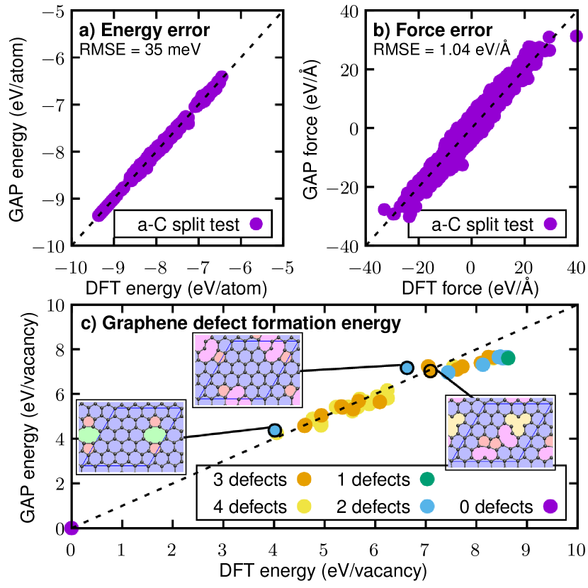
Figure 1: Accuracy benchmarks of the new carbon GAP. a) Scatter plot of predicted versus observed energies in a test set split from the training set. b) Same analysis as in a) but for the force components in this case. c) Comparison of 62 graphene structures with different numbers of vacancy defects computed with DFT versus the GAP prediction. The structures originally contained 50 atoms and vacancy defects were introduced by removing from 1 up to 4 atoms from random sites in the lattice. The structures are then relaxed and the DFT and GAP predictions compared. The insets show three example structures, where 5-, 6-, 8-, 9- and 12-membered rings are colored in red, blue, green, pink and yellow, respectively.

To ensure that the new GAP can accurately simulate the graphitization process, we performed some benchmarks as summarized in Fig. 1. We note that the root mean-square errors (RMSEs) on the “split test set” configurations (atomic configurations generated similarly to those used for training but that are excluded from the fit and reserved for testing) are smaller than those of the original GAP17. On the same test set, the new GAP reduces the error by 26% and 9% on energies and forces, respectively, as compared to GAP17. A more application-specific accuracy test was run with the new GAP for the vacancy defect formation energies in a graphene sheet. An accurate determination of these energies is critical because the graphitization process consists essentially of rearrangement of C atoms preferentially into 6-membered rings, with any deviation constituting a defect and thus incurring an energy penalty. The resulting ring and defect distribution in our porous carbon will thus be highly sensitive to the GAP’s ability to accurately reproduce these energies. In Fig. 1 c) we show how this GAP indeed succeeds at predicting the relative vacancy formation energies of a series of representative defects in close agreement with DFT. This is a stringent transferability test since structures similar to these are not included in the training set. The RMSE for defect formation energy in graphene shown in Fig. 1 c) are 0.52 eV/defect for the new GAP and 1.41 eV/defect for GAP17. Based on our tests with this and other GAPs, we ascribe this improved transferability to the use of the new soap_turbo descriptor, which provides smoother kernels.

The GAP also reproduces the cohesive energies (Fig. 2), structural and elastic properties (Table 1) of the three most important carbon allotropes: diamond, graphite and graphene. We highlight the accurate description of interlayer vdW interaction in graphite, with the only significant deviation being the $C_{33}$ elastic constant. This is a particularly positive feature of this potential given the notorious difficulty encountered by carbon force fields to reproduce vdW binding ³¹; PBE-DFT itself fails to bind graphite at all in the absence of explicit vdW corrections.

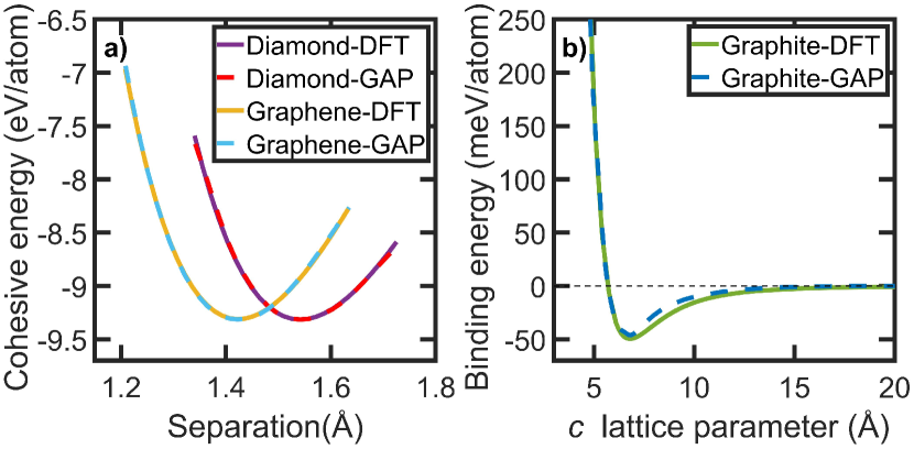
Figure 2: (a) Cohesive energy per atom versus the interatomic separation (first-nearest neighbors distance) for diamond and graphene. (b) Binding energy of graphene monolayers in graphite versus its lattice parameter $c$ (i.e., the exfoliation curve). The horizontal line is the reference for zero interaction.

Table 1: Lattice parameters (in Å) and elastic constants (in GPa) of diamond and graphite, calculated by DFT (PBE+MBD) and with the new GAP.

	Diamond		Graphite
	DFT	GAP	DFT	GAP
$a$	$3.557$	$3.560$	$2.461$	$2.463$
$c$			$6.762$	$6.803$
$C_{11}$	$1071$	$1028$	$1083$	$951$
$C_{12}$	$134$	$124$	$163$	$136$
$C_{13}$			$-4$	$4$
$C_{33}$			$35$	$129$
$C_{44}$	$582$	$538$	$5$	$7$
$C_{66}$			$460$	$407$

A crucially important aspect of the MLMD approach concerns its computational efficiency. Here we performed a comparison between the GAP17 running with LAMMPS ^{32, 33} and the new GAP running with TurboGAP for a test configuration containing 1000 C atoms (simple cubic lattice with 2 g/cm³ density and random initial velocities). We ran 1000 MD steps on a 40 CPU-core machine (the same hardware for both codes). The TurboGAP calculation ran in 0.47 CPUh or 1.7 ms/atom/MD step (42 s or 42 $\mu$s/atom/MD step of walltime) whereas the LAMMPS calculation ran in 3.3 CPUh or 12 ms/atom/MD step (297 s or 297 $\mu$s/atom/MD step of walltime), i.e., the new GAP runs about seven times faster and is more accurate. There are three main reasons for this significant speedup. First, the soap_turbo descriptors are intrinsically faster than the original SOAP because of more efficient iterative algorithms ²⁷. Second, soap_turbo implements compression, which in itself can be the single largest contribution to computational speedup in kernel-based ML potentials ³⁴. Third, TurboGAP implements efficient polynomial 3b kernels, which are also significantly faster to compute than the squared-exponential 3b kernels used in GAP17.

The result of adding the vdW correction is a computational overhead that strongly depends on the cutoff for the vdW interactions. For this benchmark comparison, a 10 Å vdW cutoff, the same as for the graphitization simulations in the next section, led to $\approx 13$ % slower TurboGAP execution (48 s, 0.53 CPUh or 1.9 ms/atom/MD step). Therefore, with the new GAP and using the TurboGAP interface, it is possible to tackle much larger systems than before which is of critical importance to achieve realistic pore sizes in the present work.

2.2 MD simulation details

We carried out all the MD simulations with the new GAP interatomic potential for carbon and the TurboGAP code ²⁹. For a comprehensive characterization of NP carbon, we performed simulations over a wide range of mass densities: $0.5$, $0.9$, $1.3$ and $1.7$ g/cm³. For each density value, a cubic simulation box with $131,072$ carbon atoms is generated with randomized initial atomic positions. The side lengths of the cubic boxes are $17.36$, $14.27$, $13.62$, and $11.54$ nm for the four densities considered above, respectively. The simulation box dimensions give an idea of the maximum pore sizes that can be modeled.

The protocol for NP carbon generation is as follows [see Fig. 3(a)]. First, we hold the highly disordered structure at a constant high temperature (9000 K) in the liquid state for 20 ps. Second, we quench the liquid with a linear decaying temperature profile for 5.5 ps down to 3500 K. The structure is then kept at 3500 K for 200 ps. This is the graphitization step ^{15, 16}, and the time has been specifically optimized to ensure that no significant further graphitization takes place after this period by monitoring the creation of 6-membered rings as a function of time, which is negligible after 200 ps at 3500 K [see Fig. 3(b)]. Finally, the graphitized sample is quenched down to 300 K over 3.2 ps, and annealed at 300 K for 10 ps to obtain the room-temperature structures. The velocity-rescaling Berendsen thermostat ³⁵ with time constant $\tau_{\text{t}}=100$ fs was used to control the temperature, and all GAP-MD simulations were performed under periodic boundary conditions within fixed box dimensions, with a Verlet integration time step of 1 fs.

For each density we performed six independent MD simulations as described above to assess the effect of individual random-seed structures on the final results. This is not needed for studying short-range structural properties such as coordination statistics, but is needed for accurate calculations of medium- and long-range structural properties such as ring statistics and pore-size distribution, as well as elasticity.

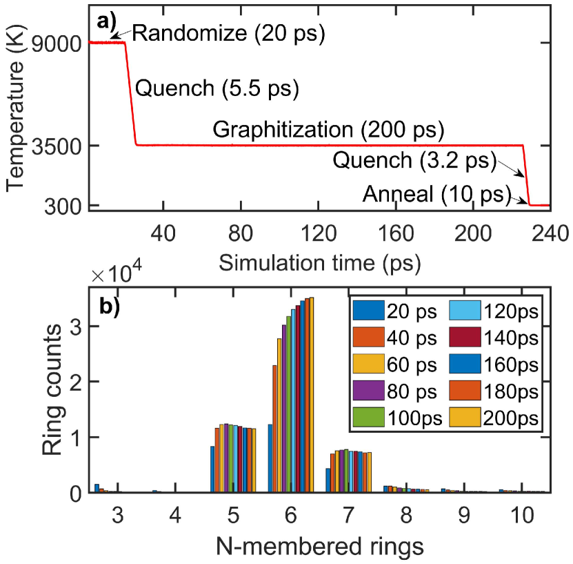
Figure 3: (a) Temperature profile during the melt-quench process. (b) Convergence of the number of $N$-membered rings ($3\leq N\leq 10$) during graphitization at $3500$ K in the system with density $0.5$ g/cm³. The number of 6-membered rings initially grows very fast, significantly slowing down towards the 200 ps mark.

2.3 Structural characterization

After obtaining the MD trajectories we used OVITO ³⁶ to calculate the radial distribution function (RDF) and the angular distribution function (ADF). The cutoff distance here was chosen as $2.0$, $1.9$, and $1.8$ Å at $9000$, $3500$, and $300$ K, respectively. This software was also used to render the structural images and calculate the coordination numbers of the $sp$, $sp^{2}$ and $sp^{3}$ structural motifs using a cutoff distance of $1.8$ Å, which fully encloses the first-neighbors shell for NP carbon. We used a single frame to calculate the RDF and ADF which is sufficient ^{37, 38} for systems with a large number of atoms.

The reciprocal-space diffraction scattering patterns, I(Q), were calculated using the Debye scattering equation as implemented in the Debyer code ³⁹:

$$I(Q)=\sum_{i}\sum_{j}f_{i}f_{j}\frac{\sin(Qr_{ij})}{Qr_{ij}}.$$ (2)

Here, $Q=4\pi\sin(\theta)/\lambda$ is the scattering parameter, where $\theta$ is the diffraction half-angle, $\lambda$ is the wavelength (1.5406 Å for the commonly used Cu $K$-$\alpha$), $r_{ij}$ is the distance between atoms $i$ and $j$, and $f$ is the atomic scattering factor for a single carbon atom. As noted in Ref. 37, the minimum image convention causes problems when using the Debye equation, and therefore it is necessary to map the atoms into the primitive cell and treat the structure as an isolated cluster.

The coordination numbers only account for short-range structural properties. To study the medium-range structural properties, we calculated ring statistics, using the shortest-path algorithm of Franzblau ⁴⁰ as implemented in the I.S.A.A.C.S. code ⁴¹. We used the same cutoff distances for nearest neighbors as in the calculation of the ADF.

To quantitatively characterize the nanopore structures arising in our samples, we calculated the size and shape distributions of the pores using the zeo++ code ⁴². For the pore size, first the three-dimensional Voronoi network⁴³ is computed to establish the void space accessibility within the pores, using the Voronoi decomposition method implemented in the Voro++ library ⁴⁴. We further take Monte Carlo samples to determine the accessible volume, and eventually determine the radius of the largest sphere that encloses the sampled point without overlapping any of the C atoms in the NP structures. As a complement to pore size, we also present corresponding pore-shape information using a stochastic ray-tracing algorithm ⁴⁵ that shoots random rays through the accessible volume of the Voronoi cell until they hit the wall of constituent C atoms. We take a probe radius of 0.7 Å (half of the typical bond length in the NP carbon samples) and 130,000 points for Monte Carlo sampling.

3 Results and discussion

3.1 Short-range order in liquid and NP carbon

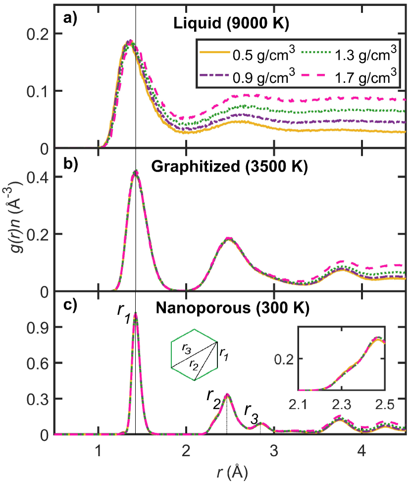
Figure 4: Density-scaled radial distribution functions $g(r)n$, where $n$ is the particle density, for (a) liquid, (b) graphitized, and (c) NP carbon structures. The insets in (c) give i) the illustration for the first three peak positions in a graphene/graphite hexagon, and ii) a magnified view in the $r$ range from 2.1 to 2.5 Å, where a small shoulder at $r$ $\approx$ $2.32$ Å indicates the presence of pentagons in the NP structure. The vertical lines mark the first three nearest-neighbor distances of $1.42$ ($r_{1}$), $2.46$ ($r_{2}$) and $2.84$ Å ($r_{3}$).

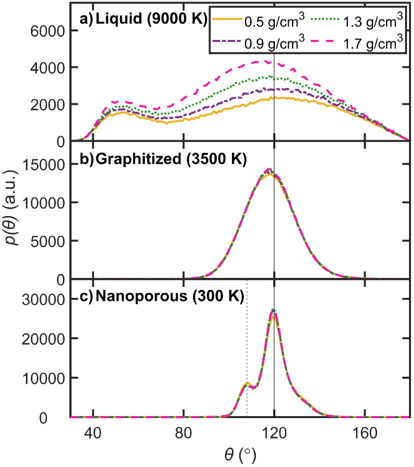
Figure 5: Angular distribution functions for (a) liquid, (b) graphitized, and (c) NP carbon structures. The solid and dashed vertical lines represent the angles for 120$\degree$ hexagons and 108$\degree$ pentagons, respectively.

To characterize the short-range order, we present the RDFs for the liquid (9000 K), graphitized (3500 K) and NP (300 K) structures generated during the melt-quench process in Fig. 4. We consider the product of RDF $g(r)$ and density of particles n to highlight the comparison between the different density systems. The RDFs converge to their respective average density of particles $n$ ($0.025$, $0.045$, $0.065$ and $0.085$ Å^-3 for $0.5$, $0.9$, $1.3$ and $1.7$ g/cm³, respectively) as the interatomic distance $r$ tends to infinity.

Similar to the results obtained by GAP17 ¹⁹, the liquid structures in Fig. 4(a) are less strongly ordered and more diffuse, showing a nonzero minimum at $\approx$ $2.0$ Å, whereas the solid phases in Fig. 4(b) and (c) are more ordered even in the medium-range regions, exhibiting more individual peaks. These solid phases, especially at 300 K, display a clear gap between their first ($r_{1}\approx$ $1.42$ Å) and second ($r_{2}\approx$ $2.46$ Å) peaks. Compared to the solid structures, in the high-temperature liquid in Fig. 4(a) the peak shifts to a smaller $r$ ($\approx$ $1.35$ Å), which is also associated with the presence of a bimodal angular distribution in the corresponding ADFs of Fig. 5(a).

After the 3500 K structure is quenched down to room temperature, the peak at $r_{3}\approx$ $2.84$ Å becomes clearly noticeable in Fig. 4(c), which corresponds to the third nearest-neighbor distance in a graphite hexagon. That the first three peak positions show a close correspondence to the first three neighbor distances of graphite implies 6-membered rings are the dominant short-range structural motif in these NP structures. Also, in the locally magnified view of Fig. 4(c), a small shoulder at $\approx$ $2.32$ Å (corresponding to the second nearest-neighbor distance in a carbon pentagon) appears in the early second nearest-neighbor region, a signature of the presence of some 5-membered rings.

To accompany the discussion with a coordination analysis of the first nearest-neighbor regions of RDF above, we give ADFs in Fig. 5. At 9000 K, in addition to the main peak at $\approx$ $120\degree$, an additional smaller one appears at $\approx$ $53\degree$ (close to the 60° in an equilateral triangle, Fig. 5(a)), which means there are some irregular triplets in existence in the liquid state. These irregular triplets might be the main cause for the shifted RDF peak in 4(a). We also note sizable differences in their ADFs across the four sampled densities in the liquid state. This is in contrast to the graphitized [Fig. 5(b)] and room-temperature NP [Fig. 5(c)] samples, for which the coordination statistics show very little dependence on the sample density. This is a clear sign that the short-range order in NP carbon is rather independent of mass density.

For the liquid samples, the ADF values all tend to zero at $180\degree$, indicative that there is almost no presence of flat linear $sp$-bonded chains. The most stable linear $sp$ chains in solid carbon are expected to show bond angles in the vicinity of 155° ⁴⁶, where the ADF in [Fig. 5(a)] is still sizable. Our present result is inconsistent with previous findings for simulated liquid carbon ^{19, 47}, in which small-size systems containing 216 atoms were modeled under period boundary conditions. Our tests indicate that this discrepancy is due to small inaccuracies at very high temperature for the energetics of linear chains as predicted by our GAP, which is biased towards the more stable bent chains ($\sim 155$°) observed at low temperature.

During the graphitization step, in Fig. 5(b), unstable triplets rearrange into more stable motifs centered at $\approx$ $120\degree$. We can clearly see the signature of near-complete graphitization, which mirrors the main structural feature of graphite hexagons. Notably, in quenched NP carbon [Fig. 5(c)], there is a new minor twin peak at 108$\degree$, which corresponds to pentagonal motifs. This is strong evidence, further supported by the ring analysis carried out later in this section, of the presence of defective 5-membered rings in quenched NP carbon. Pentagon and heptagon units play an important role in curving graphene fragments in NP and glassy carbons ⁴⁸.

3.2 Morphology and short- and medium-range characterization of NP structures

Figure 6: Cross-sectional slices ($1.5$ nm in thickness) of typical snapshots of NP carbon at the densities of (a) 0.5, (b) 0.9, (c) 1.3 and (d) 1.7 g/cm³, as well as a (e) 3D snapshot of 0.5 g/cm³. Indicated (f) $sp$ and (g, h) $sp^{3}$ motifs in the network of NP carbon. The $sp$, $sp^{2}$ and $sp^{3}$ motifs are rendered in blue, green and red, respectively. Bonds with lengths shorter than $1.8$ Å are displayed.

Density	$sp$ (%)	$sp^{2}$ (%)	$sp^{3}$ (%)
$0.5$	$3.00$ ($0.10$)	$96.59$ ($0.10$)	$0.41$ ($0.03$)
$0.9$	$2.29$ ($0.08$)	$97.07$ ($0.06$)	$0.63$ ($0.06$)
$1.3$	$1.87$ ($0.06$)	$97.38$ ($0.05$)	$0.74$ ($0.03$)
$1.7$	$1.39$ ($0.04$)	$97.68$ ($0.09$)	$0.92$ ($0.05$)

Table 2: Coordination fractions of $sp^{n}$ ($1\leq n\leq 3$) bonds versus different mass densities (g/cm³). Standard deviations are given in parentheses.

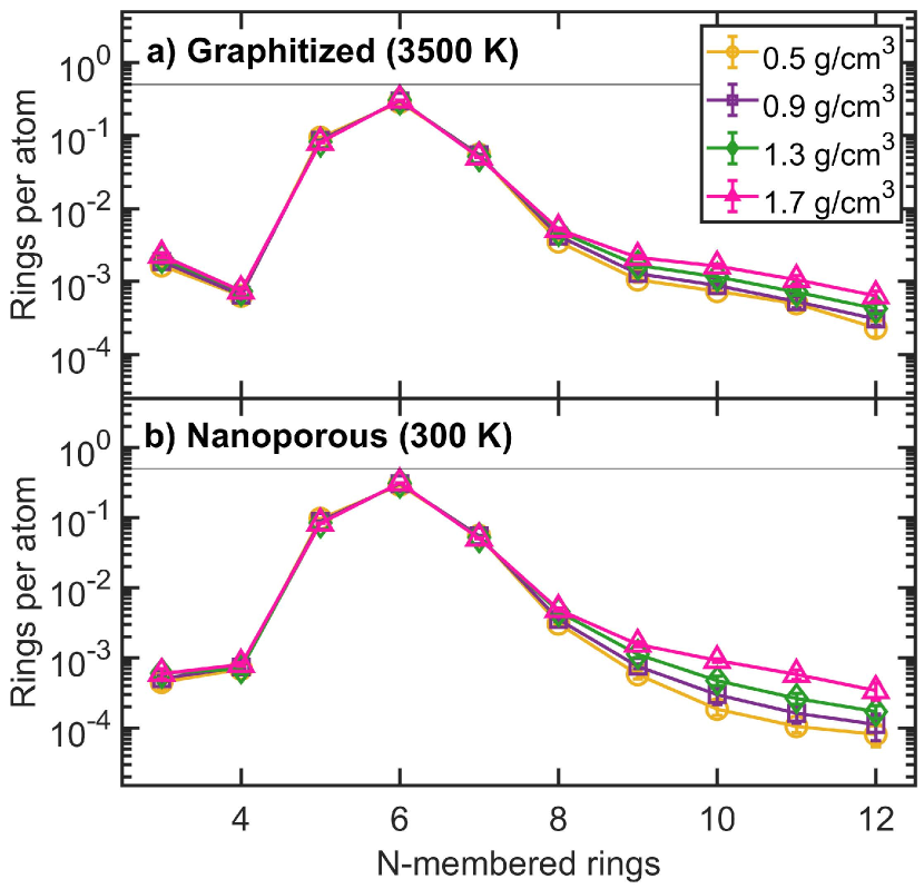
Figure 7: Number of rings per atom in (a) graphitized (3500 K) and (b) quenched (300 K) structures. The solid line indicates the reference value of 6-membered rings per atom in ideal bulk graphite. Standard deviations are given over six random seeds in simulations.

Figure 6 shows the cross-sectional morphology of our quenched NP carbon samples for the four densities studied. Clearly, most of the carbon in these samples makes up curved graphene fragments with predominantly $sp^{2}$ bonding, quantified in Table 2. These fragments assemble into three-dimensional networks, where edges contain $sp$ motifs and planes can become interlinked through $sp^{3}$ motifs (cf. Fig. 6(e-h)), which is the same role played by interstitial defects in graphite ⁴⁹. One of the distinctive characteristics of NP carbon is the typical nanostructuring of the various tangled graphitic ribbons and graphene sheets, as shown in Fig. 6. Obviously, the mass density is the main factor determining the pore sizes, with large open pores observed at low density and tightly packed graphitic planes interlinked to each other at high density. Due to their importance for emerging and established applications, pore-size distributions merit further discussion. We give an in-depth analysis of pore morphology later in this section.

For all densities, 6-, 5- and 7-membered rings, in that order, are the main repeat units making up the individual graphene layers as quantified in Fig. 7 through ring statistics. Ring statistics as a measure of the structural topology is useful to characterize medium-range order and even to reflect the curvature of the graphitic planes. Figure 7 shows the number of rings normalized per atom, from triangles to dodecagons, for all four densities studied, in both high-temperature graphitized and room-temperature NP carbon samples. As a reference point, ideal graphene or graphite has 0.5 hexagons per atom and zero curvature. Consistent with the extremely high $sp^{2}$ fraction reported in Table 2, our results show a predominance of hexagons over other rings, with an average count of 0.304 (0.299 at 3500 K). The second most common ring motif is pentagons with 0.088 rings/atom (0.086 at 3500 K), followed by heptagons with 0.054 rings/atom (0.053 at 3500 K). 6-, 5- and 7-membered rings are practically the only ring motifs contributing to the morphology of NP carbon, with the next most common motif (octagons) over two orders of magnitude less abundant than hexagons. Many of the unstable defect rings that remain after 200 ps of graphitization heal after quenching to 300 K, in particular the 3-membered rings. Ring distributions are very similar across all four densities except for larger rings, where differences are only noticeable because of the logarithmic scale used in Fig. 7. We also note that the small standard deviation (computed from the different random seeds employed at each density) confirms the robustness of the simulation protocol. Therefore, we conclude from our results that ring statistics have no density dependence.

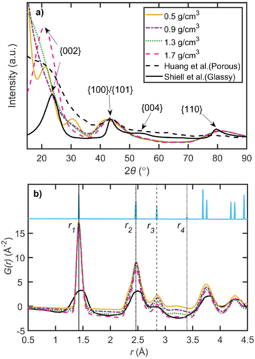
Figure 8: (a) Diffraction patterns and (b) reduced partial distribution functions $G(r)$, from our calculations and the experimental results for the HTW2500 sample ^{38, 50} and a NP carbon sample ⁵¹. The reflection indices are indicated in (a) and the $n$th nearest neighbor distances $r_{n}$ ($1\leq n\leq 4$) are represented as vertical lines in (b). For comparison, we also present results for graphite computed with $122,880$ atoms and lattice parameters of $a=2.46$ Å and $c=6.80$ Å.

In order to ensure the validity of the NP carbon structures obtained here, it is of great importance to assemble the evidence by calculating several key structural and mechanical indicators and comparing them with experimental data. Among them, diffraction patterns and radial distribution functions, $G(r)$ , are direct tools to characterize the similarity between simulated and experimentally synthesized structures. For the sake of a robust comparison, the experimental GC sample HTW2500 reported in Ref. 50 and a NP carbon sample reported in Ref. 51 are chosen. Figure 8 presents (a) the intensity of X-ray diffraction (XRD) and (b) the $G(r)$ of the reference experimental samples and our simulated NP samples. We take the 1.7 g/cm³ model structure as the closest to HTW2500, because of the similarity in mass density. The labeled peaks in Fig. 8(a) are indexed according to the graphite peaks. The HTW2500 sample has three main peaks at $2\theta\sim 24$, $44$ and $80$°, which correspond to the graphite {002}, {100} and {110} reflections. For the lower density model structures, no {002} reflection appears due to lower irregular overlapping caused by its more open and diffuse distribution of graphene sheets.

The interlayer separation can be estimated from Bragg’s law according to the relation for the $l$th-order reflection:

$$d_{00l}=\frac{l\lambda}{2\sin(\theta_{00l})},$$ (3)

where $d_{00l}$ gives the interplane separation, $\lambda$ is the wavelength of the X-ray light source and $\theta_{00l}$ is the diffraction half angle at which the $\{00l\}$ peak is observed. The shift toward smaller scattering angles in Fig. 8(a) as the density decreases is a clear sign of increasing interlayer spacing, as expected from Eq. (3). Only our computational NP sample of 1.7 g/cm³ shows a clearly defined peak for the $\{002\}$ reflection. From this peak position, $\theta\approx 21^{\circ}$, we can infer an average interlayer spacing of around 4.2 Å. There is no shift in the position of the $\{100\}$ reflection, indicating an in-plane lattice parameter $a$ of around 2.43 Å (or 1.40 Å interatomic distance) for $2\theta_{100}\approx 43^{\circ}$.

The typical size of crystallites can also be inferred from the XRD patterns with the Scherrer equation ⁵²:

$$L=\frac{K\lambda}{B(2\theta)\cos(\theta)},$$ (4)

where $K\approx 1$ is the Scherrer constant and $B(2\theta)$ is the FWHM (in radians) of a given peak on the XRD pattern. The size of in-plane “crystalline” pockets can be inferred from the data for all densities, and it is $L_{a}\approx 4$ Å for all of them. This number gives an idea of the typical regions in a graphitic sheet free of defects, i.e., made of hexagonal rings only. This quantity is in good agreement with the experimental porous sample which we compare to ours in Fig. 8. The size of crystallites along the direction of stacking can only be inferred for our 1.7 g/cm³ NP sample, as $L_{c}\approx 9$ Å. Therefore, in this sample the graphitic sheets are stacked locally similarly to a graphite crystal within length scales encompassing about three layers.

3.3 Pore-size distribution

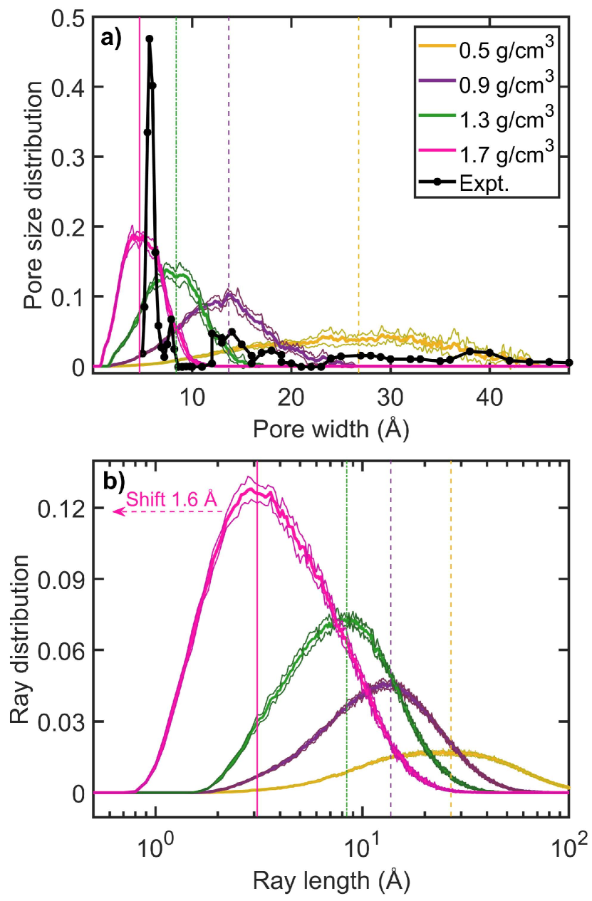
Figure 9: (a) Distribution of pore size as a function of pore width. Vertical lines mark diameters of 4.7 in pink, 8.4 in green, 13.7 in purple and 26.8 Å in brown for the decreasing order of densities. (b) Distribution of the number of rays as a function of ray length. Vertical lines mark the ray lengths of 3.1 in pink, 8.4 in green, 13.7 in purple and 26.8 Å in brown for the decreasing order of densities. Standard deviations are provided over six random seeds in the simulations.

Porosity is one of the most significant properties of NP carbons and the one that determines their usefulness for many technological applications. Therefore, the characterization of porosity and pore structures in our computational samples is a central part of this work. The normalized pore-size distribution (PSD) and ray-trace histogram are both plotted in Fig. 9. Comparison to experimental observations is challenging because of the difficulty in directly measuring PSD in experiments. In Fig. 9(a), the PSD histograms behave similarly to normal distributions. We can clearly see, as expected, that the PSDs shift to smaller diameters with increasing density, and their peaks appear, in decreasing order of density, at 0.47, 0.84, 1.37 and 2.68 nm for 1.7, 1.3, 0.9 and 0.5 g/cm³, respectively. As shown in Fig. 6, a more open structure means more available space between graphitic planes and, consequently, the presence of larger pores. At the same time, as the density increases the PSDs become sharper (i.e., the individual pores have less variation in size).

It should be pointed out that our PSD analysis is based on a spherical approximation to pores and highly sensitive to small changes in the pore diameter. It does not reflect subtle changes in surface texture features such as pore shape ⁴². To this end, stochastic ray tracing analysis, as complementary information for pore structure determination, is also shown in Fig. 9(b). Following the trend in PSDs, sharper peaks appear at smaller ray length for denser samples. In general, the low density of NP carbon explicitly gives a long trailing ray length, which is mainly caused by open structures, where some rays can travel freely through continuously connected pores until reaching the wall of a pore. Their peaks appear, in decreasing order of density, at 0.31, 0.84, 1.37 and 2.68 nm ray length for 1.7, 1.3, 0.9 and 0.5 g/cm³, respectively. Especially for lower densities, the fact that the PSD peak position is almost the same as that of ray trace indicates that a localized enclosed spherical pore curvature is the dominant morphological feature in the samples modeled. This observation agrees with the experimental prediction for the existence of spherical rather than channel-like or cylindrical-like void regions in GC ⁵⁰. This result might be related to the excess of 5-membered rings as compared to their 7-membered counterparts, because the former leads to positive curvature preferring to form closed spheres. Note that one of the most common crystallographic defects in graphene, the Stone-Wells defect, ⁵³ involves the direct substitution of four 6-membered rings with two 5-membered and two 7-membered rings. 5- and 7-member rings arising in pairs allow to maintain the planarity of the graphitic sheets, therefore, an excess of either type of ring will lead to curving of the graphitic planes. An extreme limit of this is the C₆₀ fullerene, where only 5- and 6-membered rings are present. Moreover, the peak of ray distribution for the 1.7 g/cm³ sample shifts slightly (by 1.6 Å) to its corresponding PSD value, which is due to the local interstitial space between graphitic planes. This suggests the presence of some pockets of crystallites, i.e., oriented stacked graphitic sheets, in the 1.7 g/cm³ sample. This is also evidenced by the {002} reflection in the XRD patterns and its size evaluation via the Scherrer equation above.

Finally, we note that, as in the case for ring counts, the good agreement (standard deviations visible only at the peak of the PSDs) between the six individual random-seed runs for each density gives confidence in the robustness of the simulation protocol.

3.4 Elastic properties

Under realistic conditions materials are subjected to different levels of mechanical stress. If the material’s response to stress is poorly understood, this can lead to unexpected or unwanted effects, or even to catastrophic consequences such as material failure. Thus, understanding the mechanical properties of disordered graphitic carbons is of central importance with regard to their technological and industrial applications. Therefore, we have evaluated the elastic properties of our simulated NP carbon samples and characterized the density dependence of bulk, shear and Young’s moduli. Six independent random seeds for each mass density were used to obtain good statistics for the elastic moduli of NP carbon. To assess the degree of isotropy in our samples, we computed the triclinic stiffness tensor of the material, which has 36 independent components, and then performed an isotropic projection. This projection is carried out according to the Moakher and Norris (MN) method ⁵⁴ with rotation optimization, as implemented in the Mattpy code ^{55, 56, 57}. In addition to the ability to carry out a projection, the MN method provides a quantitative measure of the similarity between the original tensor and its projection based on Euclidean distances. In this way, we can establish the degree to which finite-size effects, on the one hand, and anisotropy, on the other, are present in our samples. Finite-size effects are a consequence of the limited number of atoms in the simulation, whereas elastic anisotropy in graphitic carbons car arise if there is a preferential orientation of the graphitic planes, as occurs in crystalline graphite.

The relations between the elastic constants that are fulfilled by isotropic materials are:

$$C_{11}=C_{22}=C_{33};\qquad C_{12}=C_{13}=C_{23};$$

$$C_{44}=C_{55}=C_{66};\qquad C_{44}=(C_{11}-C_{12})/2.$$ (5)

These relations are only valid for three-dimensional isotropy. When a material displays only in-plane isotropy, only the shear, axial and biaxial elastic constants along that particular plane satisfy this relation. For instance, in crystalline graphite the elastic isotropy relations for $c$-plane isotropy are expressed by $C_{11}=C_{22}$ and $C_{66}=(C_{11}-C_{12})/2$.

The bulk ($B$), shear ($G$) and Young’s ($E$) elastic moduli, which are more commonly reported in the materials and engineering literature than the $C_{ij}$, are given for isotropic materials as a function of the elastic constants as follows:

$$B=(C_{11}+2C_{12})/3;$$ (6)

$$G=C_{44},$$ (7)

and

$$E=1/S_{11}=9BG/(3B+G),$$ (8)

where the compliance matrix S is obtained by inverting the $6\times 6$ matrix of elastic constants C.

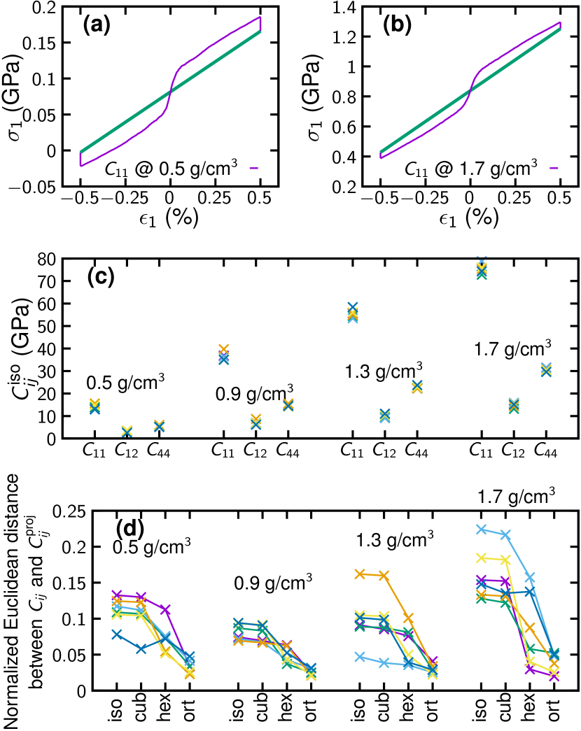
Figure 10: Two examples for 0.5 g/cm³ (a) and 1.7 g/cm³ (b) samples for the calculation of $C_{11}$, given by the relation between the stress along $x$, $\sigma_{1}$, and the strain along the same axis, $\epsilon_{1}$. (c) Isotropic projection (which gives $C_{11}$, $C_{12}$ and $C_{44}$) of the 36-component $C_{ij}$ tensor computed for all computational NP samples. (d) Normalized distance between the triclinic stiffness tensor of the samples and the isotropic (iso), cubic (cub), hexagonal (hex) and orthorhombic (ort) projections; lines connect the data corresponding to the same sample.

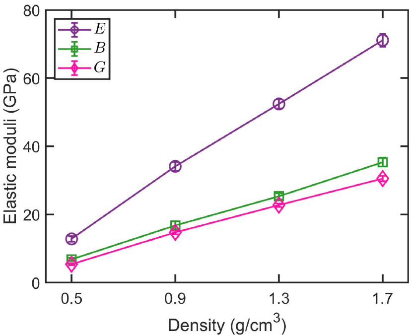
Figure 11: Average Young’s ($E$), bulk ($B$) and shear ($G$) moduli as a function of density for NP carbons. Standard deviations are given over six random seeds.

	0.5 g/cm3	0.9 g/cm3	1.3 g/cm3	1.7 g/cm3
$C_{11}^{\text{iso}}$ (GPa)	$14.0\pm 0.9$	$36.4\pm 1.7$	$55.5\pm 1.6$	$76.0\pm 2.2$
$C_{12}^{\text{iso}}$ (GPa)	$3.1\pm 0.4$	$6.9\pm 0.8$	$10.1\pm 0.7$	$15.0\pm 0.9$
$C_{44}^{\text{iso}}=G$ (GPa)	$5.4\pm 0.3$	$14.7\pm 0.5$	$22.7\pm 0.5$	$30.5\pm 0.8$
$B$ (GPa)	$6.8\pm 0.5$	$16.8\pm 1.1$	$25.3\pm 0.9$	$35.3\pm 1.3$
$E$ (GPa)	$12.8\pm 0.8$	$34.1\pm 1.3$	$52.4\pm 1.3$	$71.1\pm 1.9$
$C_{11}^{\text{hex}}/C_{33}^{\text{hex}}$	$1.07\pm 0.21$	$1.05\pm 0.15$	$1.00\pm 0.20$	$1.41\pm 0.16$

Table 3: Average isotropic elastic constants and elastic moduli, as well as ratio of hexagonal axial elastic constants, as a function of NP carbon density. The given errors are the standard deviation across random seeds in the simulations.

Because of the complexity of these materials the calculation of the stiffness tensor is not straightforward. We proceed in the following way. First, the 300 K structures are further quenched down to close to 0 K to avoid the presence of thermal noise when computing the stress tensor. Second, we slowly deform the simulation box by applying a total of $\pm 0.5$ % strains over 1 ps in each direction for all six independent strains, $\epsilon_{j}=\epsilon_{1},...,\epsilon_{6}$. This is followed by an energy minimization with a gradient descent algorithm at the strain end points. We monitor the six independent components of the stress tensor $\sigma_{i}=\sigma_{1},...,\sigma_{6}$ as a function of these deformations. This allows us to compute the elastic constants from the relation $\sigma_{i}=\sum_{j}C_{ij}\epsilon_{j}$ by assuming a linear evolution as given by the end points. Two examples of these calculations are given in Fig. 10 (a,b). As can be observed, there is a delayed elastic response in time, indicated by the non-linear dependence of the stress on the strain. The vertical lines at the end points show how the stress is relaxed at fixed strain during the energy minimization step. The thick straight lines connect the end points of the stress-strain curve, and give the time-independent elastic response of the material. In the limit of an infinitely slow deformation the non-linear curves will approximately converge towards the straight lines. Third, to estimate the isotropic elastic constants, we carry out an isotropic projection of the triclinic stiffness tensor by minimizing the Euclidean distance between the two, constrained to the symmetry of the isotropic stiffness tensor ^{54, 56, 55}, which yields the following appropriately weighted averages:

$$C_{11}^{\text{iso}}= \frac{6}{30}(C_{11}+C_{22}+C_{33})$$

$$+\frac{2}{30}(C_{12}+C_{13}+C_{23})$$

$$+\frac{8}{30}(C_{44}+C_{55}+C_{66}),$$ (9)

$$C_{12}^{\text{iso}}= \frac{2}{30}(C_{11}+C_{22}+C_{33})$$

$$+\frac{4}{30}(C_{12}+C_{13}+C_{23})$$

$$-\frac{4}{30}(C_{44}+C_{55}+C_{66}),$$ (10)

$$C_{44}^{\text{iso}}= \frac{2}{30}(C_{11}+C_{22}+C_{33})$$

$$-\frac{1}{30}(C_{12}+C_{13}+C_{23})$$

$$+\frac{6}{30}(C_{44}+C_{55}+C_{66}).$$ (11)

Note that a naive averaging of $C_{11}$, $C_{12}$ and $C_{44}$ does not generally produce a tensor with the correct symmetry. All the results are shown in Fig. 10 (c). Fourth and last, we compute the Euclidean distance between the triclinic tensor and tensors of isotropic, cubic, hexagonal and orthorhombic symmetry (listed in decreasing order of symmetry), with results shown in Fig. 10 (d). This approach allows us to establish the best candidate for the underlying symmetry of each sample.

From Fig. 10 (c), we can observe the smooth evolution of the elastic constants as a function of mass density, and also appreciate the degree of variability across samples with the same density, which is small (circa 10 %) thanks to the large number of atoms included in these calculations. Figure 11 shows the average computed for each density, presented in this case in the form of elastic moduli. All of these values are also summarized in Table 3.

Going back to Fig. 10 (d) we observe the general expected trend that as the symmetry of the projection is lowered, the original triclinic tensor can be better accommodated (the distance between $C_{ij}$ and $C_{ij}^{\text{proj}}$ decreases). These results also tell us that there is, loosely speaking, between 5 % (one of the samples at 1.3 g/cm³) and 23 % (one of the samples at 1.7 g/cm³) discrepancy between the triclinic tensor and its isotropic projection. Some valuable information can be extracted by comparing the hexagonal projection to both cubic (or even isotropic) and orthorhombic. If the hexagonal projection is very close to the orthorhombic projection and they are both relatively far away from the cubic one, there is indication of an underlying hexagonal elastic response. As we have discussed earlier, the most characteristic feature in terms of elasticity of hegaxonal lattices is the existence of an isotropy plane. In other words, these NP samples would show preferential stacking of graphitic planes along a particular axis. We can see in Fig. 10 (d) that at low densities the transition from cubic to hexagonal to orthorhombic projections is smooth, whereas at higher densities some of the samples show an abrupt transition. This effect can be further quantified by computing the ratio $C_{11}^{\text{hex}}/C_{33}^{\text{hex}}$, where, as this quantity deviates from unity (usually towards larger values), the existence of a preferential direction is further emphasized. This effect is quantified in Table 3, where the highest density samples show $C_{11}^{\text{hex}}$ approximately 40 % larger than $C_{33}^{\text{hex}}$. This is indicative of a small degree of “graphite-likeness” in these samples, which is expected to increase further with density. We note, however, that for our computational NP carbon samples this ratio is still much smaller (by two orders of magnitude) than that of crystalline graphite. In addition, the effect is likely due to finite-size effects, and will probably become even less pronounced for bigger systems. We therefore conclude that these computational samples are for most practical purposes elastically isotropic.

4 Conclusions

In summary, we have carried out a comprehensive computational study of the atomistic structure, pore-size distribution and elastic properties of NP carbons in the mass density range from 0.5 g/cm³ to 1.7 g/cm³. Realistic simulations of these NP carbon structures, including the modeling of nanopore sizes up to 40 Å in diameter, have been made possible through the combination of large simulation cells containing 131,072 atoms each, and the utilization of an accurate and fast GAP force field for carbon including van der Waals interactions. The new GAP potential and the generated NP carbon structures are freely available to the community ^{30, 58}.

The structural analysis reveals that at all densities studied these NP carbons are made up mostly of graphitic planes, with circa 97 % of all atoms being $sp^{2}$ bonded. Graphitic planes are interlinked via $sp^{3}$ motifs, whose concentration increases twofold from 0.5 g/cm³ (0.5 %) to 1.7 g/cm³ (1.1 %). Some of the graphitic planes are terminated with edges involving the presence of $sp$ motifs, whose concentration follows the opposite trend to that of $sp^{3}$ motifs (from 3 % at 0.5 g/cm³ down to 1.4 % at 1.7 g/cm³). The samples are highly graphitized, with a topology clearly dominated by 6-membered rings, followed in smaller quantities by 5- and 7-membered rings, in that order. By comparison, the presence of smaller or larger rings is negligible, with the next most common ring motif, 8-membered rings, being more that two orders of magnitude rarer than the 6-membered rings.

The radial distribution functions for all densities show well-defined peaks for first, second and third nearest neighbors corresponding to those of graphite, with the most remarkable feature being a sizable broadening of the second-neighbors peak. This corresponds to the presence of 5-membered rings in the samples. The angular distribution function correspondingly shows a bimodal distribution, with the largest peak centered around 120° (hexagonal motifs) and a second smaller peak centered around 108° (pentagonal motifs). A small tail also appears for angles larger than 120° (heptagons and beyond). The calculated XRD patterns show the expected trends with density and offer a direct route for comparison with experiment.

The pore-size analysis reveals bell-shaped distributions whose center and width shift towards larger values as the density decreases. Typical nanopore diameters increase from 5 Å at 1.7 g/cm³ up to 27 Å at 0.5 g/cm³. Interestingly, small nanopores are very rare in the low-density NP carbon samples. This is indicative of homogeneous nanopore size distributions for a sample of a given density.

Finally, our analysis of elasticity showed that the samples behave mostly isotropically from a mechanical perspective, with the degree of elastic isotropy slowly decreasing with density. The elastic moduli of the material increase monotonically with density, and the Young’s modulus increases more rapidly than bulk or shear moduli. The elastic response of these NP carbons increased by roughly an order of magnitude from 0.5 g/cm³ to 1.7 g/cm³, with the elastic constants of the latter still more than an order of magnitude smaller than those of diamond.

We hope that the detailed insight into the atomic structure of NP carbon materials provided in this work will inspire and guide future experimental efforts, especially for energy-storage applications. We also expect that the library of atomic structures provided to the research community will serve as a starting point for future computational studies on the electronic, structural and mechanical properties of NP carbon.

The authors acknowledge funding from the Academy of Finland, under projects 321713 (M.A.C. & Y.W.), 330488 (M.A.C.), 312298/QTF Center of Excellence program ( T.A.-N., Z.F. & Y.W.), and the China Scholarship Council under grant no. CSC202006460064 (Y.W.). The authors also acknowledge computational resources from the Finnish Center for Scientific Computing (CSC) and Aalto University’s Science IT project.

References

- Kärger 2015 Kärger, J. Transport phenomena in nanoporous materials. Chem. Phys. Chem. 2015, 16, 24
- Laurila et al. 2017 Laurila, T.; Sainio, S.; Caro, M. A. Hybrid carbon based nanomaterials for electrochemical detection of biomolecules. Prog. Mater. Sci. 2017, 88, 499
- Li et al. 2020 Li, Z.; Xu, J.; Sun, D.; Lin, T.; Huang, F. Nanoporous carbon foam for water and air purification. ACS Appl. Nano Mater. 2020, 3, 1564
- Wang et al. 2021 Wang, G.; Yu, M.; Feng, X. Carbon materials for ion-intercalation involved rechargeable battery technologies. Chem. Soc. Rev. 2021, 50, 2388
- Vix-Guterl et al. 2005 Vix-Guterl, C.; Frackowiak, E.; Jurewicz, K.; Friebe, M.; Parmentier, J.; Béguin, F. Electrochemical energy storage in ordered porous carbon materials. Carbon 2005, 43, 1293
- Odom et al. 1998 Odom, T. W.; Huang, J.-L.; Kim, P.; Lieber, C. M. Atomic structure and electronic properties of single-walled carbon nanotubes. Nature 1998, 391, 62
- Geim and Novoselov 2007 Geim, A.; Novoselov, K. The rise of graphene. Nature materials 2007, 6, 183
- Purohit et al. 2014 Purohit, R.; Purohit, K.; Rana, S.; Rana, R. S.; Patel, V. Carbon nanotubes and their growth methods. Proc. Mat. Sci. 2014, 6, 716
- Kumar et al. 2013 Kumar, P. V.; Bernardi, M.; Grossman, J. C. The impact of functionalization on the stability, work function, and photoluminescence of reduced graphene oxide. ACS Nano 2013, 7, 1638
- Savazzi et al. 2018 Savazzi, F.; Risplendi, F.; Mallia, G.; Harrison, N. M.; Cicero, G. Unravelling Some of the Structure–Property Relationships in Graphene Oxide at Low Degree of Oxidation. J. Phys. Chem. Lett. 2018, 9, 1746
- Sundqvist 2021 Sundqvist, B. Carbon under pressure. Phys. Rep. 2021, 909, 1
- Deringer et al. 2019 Deringer, V. L.; Caro, M. A.; Csányi, G. Machine Learning Interatomic Potentials as Emerging Tools for Materials Science. Adv. Mater. 2019, 31, 1902765
- Caro et al. 2018 Caro, M. A.; Deringer, V. L.; Koskinen, J.; Laurila, T.; Csányi, G. Growth Mechanism and Origin of High Content in Tetrahedral Amorphous Carbon. Phys. Rev. Lett. 2018, 120, 166101
- Muhli et al. 2021 Muhli, H.; Chen, X.; Bartók, A. P.; Hernández-León, P.; Csányi, G.; Ala-Nissila, T.; Caro, M. A. Machine learning force fields based on local parametrization of dispersion interactions: Application to the phase diagram of C60. Phys. Rev. B 2021, 104, 054106
- de Tomas et al. 2016 de Tomas, C.; Suarez-Martinez, I.; Marks, N. A. Graphitization of amorphous carbons: A comparative study of interatomic potentials. Carbon 2016, 109, 681
- de Tomas et al. 2019 de Tomas, C.; Aghajamali, A.; Jones, J. L.; Lim, D. J.; López, M. J.; Suarez-Martinez, I.; Marks, N. A. Transferability in interatomic potentials for carbon. Carbon 2019, 155, 624
- Bartók et al. 2010 Bartók, A. P.; Payne, M. C.; Kondor, R.; Csányi, G. Gaussian approximation potentials: The accuracy of quantum mechanics, without the electrons. Phys. Rev. Lett. 2010, 104, 136403
- Bartók and Csányi 2015 Bartók, A.; Csányi, G. Gaussian approximation potentials: A brief tutorial introduction. Int. J. Quantum Chem. 2015, 115, 1051
- Deringer and Csányi 2017 Deringer, V. L.; Csányi, G. Machine learning based interatomic potential for amorphous carbon. Phys. Rev. B 2017, 95, 094203
- Perdew et al. 1996 Perdew, J. P.; Burke, K.; Ernzerhof, M. Generalized Gradient Approximation Made Simple. Phys. Rev. Lett. 1996, 77, 3865
- Tkatchenko et al. 2012 Tkatchenko, A.; DiStasio Jr, R. A.; Car, R.; Scheffler, M. Accurate and efficient method for many-body van der Waals interactions. Phys. Rev. Lett. 2012, 108, 236402
- Bučko et al. 2016 Bučko, T.; Lebègue, S.; Gould, T.; Ángyán, J. G. Many-body dispersion corrections for periodic systems: an efficient reciprocal space implementation. J. Phys.: Condens. Matter 2016, 28, 045201
- Kresse and Furthmüller 1996 Kresse, G.; Furthmüller, J. Efficient iterative schemes for ab initio total-energy calculations using a plane-wave basis set. Phys. Rev. B 1996, 54, 11169
- Kresse and Joubert 1999 Kresse, G.; Joubert, D. From ultrasoft pseudopotentials to the projector augmented-wave method. Phys. Rev. B 1999, 59, 1758
- Deringer et al. 2021 Deringer, V. L.; Bartók, A. P.; Bernstein, N.; Wilkins, D. M.; Ceriotti, M.; Csányi, G. Gaussian Process Regression for Materials and Molecules. Chem. Rev. 2021, 121, 10073
- Bartók et al. 2013 Bartók, A. P.; Kondor, R.; Csányi, G. On representing chemical environments. Phys. Rev. B 2013, 87, 184115
- Caro 2019 Caro, M. A. Optimizing many-body atomic descriptors for enhanced computational performance of machine learning based interatomic potentials. Phys. Rev. B 2019, 100, 024112
- Rowe et al. 2020 Rowe, P.; Deringer, V. L.; Gasparotto, P.; Csányi, G.; Michaelides, A. An accurate and transferable machine learning potential for carbon. J. Chem. Phys. 2020, 153, 034702
- 29 The TurboGAP code. \urlhttp://turbogap.fi, accessed: 2021-05-12
- Caro 2021 Caro, M. A. GAP interatomic potential for amorphous carbon, version 2.0. Zenodo:10.5281/zenodo.5243184 2021,
- Qian et al. 2021 Qian, C.; McLean, B.; Hedman, D.; Ding, F. A comprehensive assessment of empirical potentials for carbon materials. APL Mater. 2021, 9, 061102
- Plimpton 1995 Plimpton, S. Fast parallel algorithms for short-range molecular dynamics. J. Comput. Phys. 1995, 117, 1
- 33 Large-scale Atomic/Molecular Massively Parallel Simulator. \urlhttp://lammps.sandia.gov, accessed: 2021-05-12
- Musil et al. 2021 Musil, F.; Veit, M.; Goscinski, A.; Fraux, G.; Willatt, M. J.; Stricker, M.; Junge, T.; Ceriotti, M. Efficient implementation of atom-density representations. J. Chem. Phys. 2021, 154, 114109
- Berendsen et al. 1984 Berendsen, H. J. C.; Postma, J. P. M.; van Gunsteren, W. F.; DiNola, A. R. H. J.; Haak, J. R. Molecular dynamics with coupling to an external bath. J. Chem. Phys. 1984, 81, 3684
- Stukowski 2010 Stukowski, A. Visualization and analysis of atomistic simulation data with OVITO-the Open Visualization Tool. Modelling and Simulation in Materials Science and Engineering 2010, 18, 015012
- de Tomas et al. 2016 de Tomas, C.; Suarez-Martinez, I.; Marks, N. A. Graphitization of amorphous carbons: A comparative study of interatomic potentials. Carbon 2016, 109, 681–693
- Shiell et al. 2019 Shiell, T. B.; Wong, S.; Yang, W.; Tanner, C. A.; Haberl, B.; Elliman, R. G.; McKenzie, D. R.; McCulloch, D. G.; Bradby, J. E. The composition, structure and properties of four different glassy carbons. Journal of Non-Crystalline Solids 2019, 522, 119561
- 39 Wojdyr, M. Debyer. \urlhttps://github.com/wojdyr/debyer (accessed 2021-12-12)
- Franzblau 1991 Franzblau, D. S. Computation of ring statistics for network models of solids. Phys. Rev. B 1991, 44, 4925–4930
- Le Roux and Petkov 2010 Le Roux, S.; Petkov, V. ISAACS–interactive structure analysis of amorphous and crystalline systems. Journal of Applied Crystallography 2010, 43, 181–185
- Pinheiro et al. 2013 Pinheiro, M.; Martin, R. L.; Rycroft, C. H.; Jones, A.; Iglesia, E.; Haranczyk, M. Characterization and comparison of pore landscapes in crystalline porous materials. Journal of Molecular Graphics and Modelling 2013, 44, 208–219
- Willems et al. 2012 Willems, T. F.; Rycroft, C. H.; Kazi, M.; Meza, J. C.; Haranczyk, M. Algorithms and tools for high-throughput geometry-based analysis of crystalline porous materials. Microporous and Mesoporous Materials 2012, 149, 134–141
- Rycroft 2009 Rycroft, C. H. VORO++: A three-dimensional Voronoi cell library in C++. Chaos 2009, 19, 041111
- Jones et al. 2013 Jones, A. J.; Ostrouchov, C.; Haranczyk, M.; Iglesia, E. From rays to structures: Representation and selection of void structures in zeolites using stochastic methods. Microporous and Mesoporous Materials 2013, 181, 208–216
- Caro et al. 2018 Caro, M. A.; Aarva, A.; Deringer, V. L.; Csányi, G.; Laurila, T. Reactivity of amorphous carbon surfaces: rationalizing the role of structural motifs in functionalization using machine learning. Chem. Mater. 2018, 30, 7446
- Rowe et al. 2020 Rowe, P.; Deringer, V. L.; Gasparotto, P.; Csányi, G.; Michaelides, A. An accurate and transferable machine learning potential for carbon. The Journal of Chemical Physics 2020, 153, 034702
- Martin et al. 2019 Martin, J. W.; de Tomas, C.; Suarez-Martinez, I.; Kraft, M.; Marks, N. A. Topology of Disordered 3D Graphene Networks. Phys. Rev. Lett. 2019, 123, 116105
- Li et al. 2005 Li, L.; Reich, S.; Robertson, J. Defect energies of graphite: Density-functional calculations. Phys. Rev. B 2005, 72, 184109
- Shiell et al. 2021 Shiell, T. B.; McCulloch, D. G.; Bradby, J. E.; Haberl, B.; McKenzie, D. R. Neutron diffraction discriminates between models for the nanoarchitecture of graphene sheets in glassy carbon. Journal of Non-Crystalline Solids 2021, 554, 120610
- Huang et al. 2011 Huang, W.; Zhang, H.; Huang, Y.; Wang, W.; Wei, S. Hierarchical porous carbon obtained from animal bone and evaluation in electric double-layer capacitors. Carbon 2011, 49, 838
- Scherrer 1912 Scherrer, P. Kolloidchemie Ein Lehrbuch; Springer, 1912; p 387
- Stone and Wales 1986 Stone, A. J.; Wales, D. J. Theoretical studies of icosahedral C60 and some related species. Chem. Phys. Lett. 1986, 128, 501
- Moakher and Norris 2006 Moakher, M.; Norris, A. N. The closest elastic tensor of arbitrary symmetry to an elasticity tensor of lower symmetry. J. Elasticity 2006, 85, 215
- 55 Caro, M. A. Mattpy. http://github.com/mcaroba/mattpy (accessed 2021-12-12)
- Caro 2014 Caro, M. A. Extended scheme for the projection of material tensors of arbitrary symmetry onto a higher symmetry tensor. 2014-08-06. arXiv repository. arXiv:1408.1219 (accessed 2021-12-12)
- Caro et al. 2015 Caro, M. A.; Zhang, S.; Riekkinen, T.; Ylilammi, M.; Moram, M. A.; Lopez-Acevedo, O.; Molarius, J.; Laurila, T. Piezoelectric coefficients and spontaneous polarization of ScAlN. J. Phys.: Condens. Matter 2015, 27, 245901
- Wang and Caro 2021 Wang, Y.; Caro, M. A. Nanoporous carbon structures of different densities generated through GAP molecular dynamics. Zenodo 2021, 10.5281/zenodo.5512595