Integrated Optimization of Sequential Processes: General Analysis and Application to Public Transport

Abstract

Planning in public transportation is traditionally done in a sequential process: After the network design process, the lines and their frequencies are planned. When these are fixed, a timetable is determined and based on the timetable, the vehicle and crew schedules are optimized. After each step, passenger routes are adapted to model the behavior of the passengers as realistically as possible. It has been mentioned in many publications that such a sequential process is sub-optimal, and integrated approaches, mainly heuristics, are under consideration. Sequential planning is not only common in public transportation planning but also in many other applied problems, among others in supply chain management, or in organizing hospitals efficiently.

The contribution of this paper hence is two-fold: on the one hand, we develop an integrated integer programming formulation for the three planning stages line planning, (periodic) timetabling, and vehicle scheduling which also includes the integrated optimization of the passenger routes. This gives us an exact formulation rewriting the sequential approach as an integrated problem. We discuss properties of the integrated formulation and apply it experimentally to data sets from the LinTim library. On small examples, we get an exact optimal objective function value for the integrated formulation which can be compared with the outcome of the sequential process.

On the other hand, we propose a mathematical formulation for general sequential processes which can be used to build integrated formulations. For comparing sequential processes with their integrated counterparts we analyze the price of sequentiality, i.e., the ratio between the solution obtained by the sequential process and an integrated solution. We also experiment with different possibilities for partial integration of a subset of the sequential problems and again illustrate our results using the case of public transportation. The obtained results may be useful for other sequential processes.

Keywords: public transport planning, line planning, timetable, vehicle scheduling, passenger routes, sequential process, integrated optimization, price of sequentiality

1 Introduction

Public transport planning, as described in [DH07] encompasses various planning stages, such as network design, line planning, timetabling, passenger routing, vehicle scheduling and crew scheduling. Although these stages are highly interdependent, they are usually solved sequentially with the passengers’ paths being adapted after each stage. Within the last few years, researchers noticed that this is a greedy-like approach and started working on integrated approaches instead. Also planning problems in many other fields are multi-stage optimization problems which are too complicated to be solved in an integrated manner and hence their different stages are treated sequentially. Such sequential procedures are in particular common when infrastructural decisions are involved. These are made first (finding locations, building offices, houses, or shops, inventory decisions) while in a second phase the assignment, scheduling, or routing is done. An integrated model would allow to make the infrastructural decision already in such a way that the second-stage decision is as good as possible. This applies, e.g., for the design of supply chains, for production processes, or for planning the operations in airports or hospitals. Also in these fields, researchers noticed that integrated optimization may be more beneficial than only concentrating on the single stages. For example, integrated approaches have been compared to the sequential approach in supply chain management, [KDC18] or in production-distribution systems. For the latter, [DC18] analyzes differences between the sequential steps of location, production, inventory, and distribution decisions compared to an integrated approach while [AS16, AADP⁺18] focus on the benefits of integration for the production and inventory routing problem, respectively.

In the literature, there are also a few general ideas on how to integrate different planning stages or subproblems into one optimization model for which general solution approaches can be formulated. One general scheme which allows to find a local optimum is the eigenmodel proposed in [Sch17]. Here, it is shown how to develop approaches which iteratively solve subproblems being related to the different stages of a multi-stage problem. Convergence of these iterative approaches is analyzed in [JS20]. Formulating a sequential process as one integrated optimization model is further complicated if every planning stage has its own objective function, or if the whole problem is multi-objective by definition. In these cases, defining an objective function for the integrated problem is not easy, taking all decision makers into account. It is also not clear how the quality of results should be measured. For modeling situations through interwoven or complex systems, we refer to [KMN⁺20, DKK⁺20].

In this paper we study sequential processes and how they can be integrated into one common optimization problem. We are in particular interested how much we can improve the objective function value by solving the integrated model instead of taking the sequential solution. We derive the notation, analysis and results for the general case of sequential processes but illustrate everything in the case of public transport planning where we focus on the three consecutive planning stages line planning, (periodic) timetabling, and vehicle scheduling together with finding the passenger routes. As a side-effect we present an integer programming formulation for the integrated problem of line planning, timetabling, vehicle scheduling, and passenger routing.

The remainder of the paper is structured as follows: In Section 2 we start by providing a general scheme for dealing with sequential processes. We introduce the notation needed and show how a sequential process can be transformed into an integrated formulation. While this can be written down easily, formulating such an integrated problem in a practical case may be much harder. This is illustrated by developing an integrated formulation for the sequential process of line planning, timetabling and vehicle scheduling (including passenger routing) in Section 3. This section includes a literature review on work towards integrated optimization in public transportation as well as a description of the sequential process and the integrated model for this case. In Section 4 we introduce the price of sequentiality (PoS) which is used to compare the sequential solution to an integrated solution and we derive theoretical properties for the PoS. Section 5 is devoted to the case of partial integration and its price of sequentiality. Finally, in Section 6 we show experimental results using the LinTim-library [SAS⁺, SAS⁺20]. The paper is ended by a conclusion in Section 7.

2 Sequential processes and their integration

Sequential processes and their integrated solution have been considered in [BHK17, Sch14, Sch17, KDC18, AS16] for special applications. A more general framework which is the basis for the notation used in this paper has been introduced in [Sch20]. Along these lines we start by defining a sequential process.

Definition 1.

A sequential process is given by a sequence of sequential problems $(\textup{Seq}_{i}(\bar{x}_{1},\ldots,\bar{x}_{i-1}))$, $i\in\{1,\ldots,n\}$,

$$(\textup{Seq}_{i}(\bar{x}_{1},\ldots,\bar{x}_{i-1}))\quad\min\; f_{i}(\bar{x}_{1},\ldots,\bar{x}_{i-1};x_{i})$$

s.t. $$x_{i}\in F_{i}(\bar{x}_{1},\ldots,\bar{x}_{i-1}).$$

For $i\in\{1,\ldots,n\}$ we call $(\textup{Seq}_{i}(\bar{x}_{1},\ldots,\bar{x}_{i-1}))$ stage $i$ of the sequential process. It includes $m_{i}\in\mathbb{N}$ variables $x_{i}\in\mathbb{R}^{m_{i}}$, a feasible set $F_{i}(\bar{x}_{1},\ldots,\bar{x}_{i-1})\subseteq\mathbb{R}^{m_{i}}$ and objective function $f_{i}\colon\mathbb{R}^{m_{1}}\times\ldots\times\mathbb{R}^{m_{i}}\to\mathbb{R}$.

$f_{i}$ depends not only on the variables $x_{i}\in\mathbb{R}^{m_{i}}$ of the current stage but also on the variables of previous stages. When we want to indicate that only $x_{i}$ are variables, we separate them by a semicolon and write $f_{i}(\bar{x}_{1},\ldots,\bar{x}_{i-1};\cdot)\colon\mathbb{R}^{m_{i}}\to\mathbb{R}$.

Let $(\textup{Seq}_{1})$ be feasible with optimal solution $\bar{x}_{1}$ and let $(\textup{Seq}_{i}(\bar{x}_{1},\ldots,\bar{x}_{i-1}))$ be feasible with optimal solution $\bar{x}_{i}$ for each $i\in\{2,\ldots,n\}$. Then we call

$$\bar{x}=(\bar{x}_{1},\ldots,\bar{x}_{n})$$

a sequential solution.

Let us assume that we are able to solve each of the sequential problems $(\textup{Seq}_{i}(\bar{x}_{1},\ldots,\bar{x}_{i-1}))$ for $i\in\{1,\ldots,n\}$ to optimality by known deterministic algorithms ${{\sf A}}_{1},\ldots,{{\sf A}}_{n}$. Applying these algorithms ${{\sf A}}_{1},\ldots,{{\sf A}}_{n}$ sequentially outputs a sequential solution and is hence called sequential solution approach. It is in short given by

Problem	Algorithm	Input	Output
$(\textup{Seq}_{1})$	${{\sf A}}_{1}$	$\emptyset$	$\bar{x}_{1}$
$(\textup{Seq}_{2}(\bar{x}_{1}))$	${{\sf A}}_{2}$	$\bar{x}_{1}$	$\bar{x}_{2}$
$(\textup{Seq}_{3}(\bar{x}_{1},\bar{x}_{2}))$	${{\sf A}}_{3}$	$\bar{x}_{1},\bar{x}_{2}$	$\bar{x}_{3}$
	⋮
$(\textup{Seq}_{n}(\bar{x}_{1},\bar{x}_{2},\ldots,\bar{x}_{n-1}))$	${{\sf A}}_{n}$	$\bar{x}_{1},\bar{x}_{2},\ldots,\bar{x}_{n-1}$	$\bar{x}_{n}$

Obviously, such a sequential process is a Greedy-like approach: in every stage we do the best possible. The question is if this is really the best possible for the sequential process as a whole. To give an answer we need to compare the sequential solution approach with the integrated solution approach of solving the following integrated problem.

Definition 2.

For a sequential process as in Definition 1, and weights $\lambda_{i}\geq 0$, $i\in\{1,\ldots,n\}$, the corresponding integrated optimization problem is defined as a multi-stage optimization problem

$$\textup{(MSP)}\quad\min\; f(x_{1},\ldots,x_{n})=\sum_{i=1}^{n}\lambda_{i}\cdot f_{i}(x_{1},\ldots,x_{i})$$

$$\textup{s.t.}\quad x_{1} \in F_{1}$$

$$x_{2} \in F_{2}(x_{1})$$

$$\vdots$$

$$x_{n} \in F_{n}(x_{1},\ldots,x_{n-1}).$$

An optimal solution to (MSP) is called (optimal) integrated solution.

The parameters $\lambda_{1},\ldots,\lambda_{n}$ represent how important the objective of stage $i$ is for the whole process. They can also be motivated by multi-objective optimization: Let us treat the multi-stage problem (MSP) in a multi-objective fashion. Instead of one common objective function, we then consider

$$f=\left(\begin{array}[]{c}f_{1}(x_{1})\\ f_{2}(x_{1},x_{2})\\ \vdots\\ f_{n}(x_{1},\ldots,x_{n})\end{array}\right)$$

as a vector-valued objective function. It is known (see, e.g., [Ehr05]) that for $\lambda_{i}>0$ for all $i\in\{1,\ldots,n\}$ a (supported) Pareto solution will be found, and for $\lambda_{i}\geq 0$ for all $i\in\{1,\ldots,n\}$ a (supported) weakly Pareto solution is obtained.

Clearly, the integrated solution is always better than a sequential solution.

Lemma 3.

Let $x^{*}=(x^{*}_{1},\ldots,x^{*}_{n})$ be an optimal solution to (MSP) and let $\bar{x}=(\bar{x}_{1},\ldots,\bar{x}_{n})$ be a sequential solution, i.e., $\bar{x}_{i}$ is an optimal solution to $(\textup{Seq}_{i}(\bar{x}_{1},\ldots,\bar{x}_{i-1}))$ for $i\in\{1,\ldots,n\}$. Then $f(x^{*})\leq f(\bar{x})$.

Proof.

The result directly follows from the fact that the sequential solution is a feasible solution to (MSP). ∎

Before we continue, we illustrate the notation in the example of public transport optimization.

3 The sequential planning process in public transport and an integrated formulation

In this section we develop an integrated formulation for the sequential process in public transport planning as depicted in Figure 1. The main effort for this lies in the formulation of the single planning stages as in Definition 1. These are provided in Section 3.2. The integrated formulation is then put together in Section 3.3.

Figure 1: Structure of the integrated line planning, timetabling and vehicle scheduling problem with passenger routing.

3.1 Literature review: planning in public transportation

We start by providing a short review on literature for planning in public transportation. The established sequential solution approach consists of network design, line planning, timetabling, vehicle scheduling and crew scheduling (see, e.g., [CW86, BWZ97, DH07, GH10, LLB18]). Note that other sequential approaches are also possible and under research. In [PSSS17, BSS20], a vehicle schedule is computed before the timetable while in [MS09], a vehicle schedule is constructed first, followed by lines and a timetable. For a theoretical analysis of the different sequential solution approaches, see [Sch17]. Here, we concentrate on line planning, passenger routing, periodic timetabling and vehicle scheduling as the core stages. An overview on line planning is provided in [Sch12] and on (periodic) timetabling in [Nac98, Lie06]. For vehicle scheduling we refer to [BK09]. Research still carries on for each of these stages, see [FHSS18, ŞABS20] for extensions of line planning, [BLR19, GS18, BHKL20] for new features and procedures in periodic timetabling and [BKLL18, GSYG20, GBV⁺19] for work on vehicle scheduling. We also refer to the references therein. Besides research on robustness in public transport and work on case studies, integration of the mentioned planning stages is a current topic and the focus of this paper. There exists the following literature for integrating subsets of the stages; mostly in a heuristic manner.

Integration of line planning and timetabling

In [Lie08] line segments are connected to lines during the timetabling stage in a heuristic approach. Iterative approaches of alternately re-optimizing line plans and timetables are presented in [BBVL17, YG19]. Exact integer programming models are presented in [RN09, KR13, BCHP20] and solved by a column generation approach, a cross entropy heuristic and a matheuristic, respectively.

Integration of timetabling and vehicle scheduling

While we are interested in periodic timetabling, most models for integrated timetabling and vehicle scheduling deal with aperiodic timetables and solve the resulting integrated problem heuristically. The timetable and the vehicle schedule are often optimized iteratively, see [GH10, PLM⁺13, SE15, FvdHRL18] but also with matheuristics in [CFG⁺19] or by a bi-level model in [YHWL17]. A periodic version for integrating timetabling and vehicle scheduling can be found in [vL21] while in [Lin00] periodic vehicle scheduling is integrated indirectly by using an approximation of the costs as objective. In [DRB⁺17] periodic vehicle scheduling constraints are added to a periodic event scheduling problem. Pareto solutions for integrating periodic timetabling with aperiodic vehicle scheduling are identified in [SSR20].

Integration of line planning, timetabling, and vehicle scheduling

Integrating the three steps usually takes two objectives, namely travel time for the passengers and costs of the public transport supply, into account. In [Lie08, LHS18], simplified integrated models are presented by adding further constraints to the periodic and aperiodic timetabling problem, respectively. Heuristic approaches which are based on changing the order of the sequential problems are given in [MS09, PSSS17] and generalized in [Sch17]. Finally, [PSS18] only focuses on the costs of the public transport supply with the minimal restriction that all passengers can travel.

Integration of passenger routing

Line planning has been integrated with passenger routing for nearly 15 years, starting with [SS06] including penalties for transfers. An efficient solution approach is provided by [BGP07], still, the integrated problem can only be solved for small to medium sized instances. In a capacitated setting it is especially difficult to guarantee that all passengers can travel on shortest paths, see [GS17] for integer programming formulations and [SSS19] for game theoretic approaches. The integration of timetabling with passenger routing came up later, but has been researched intensively since this time, see [SS10, SG13, Sch14, SS15, RSAMB17, BHK17, SS20, PSH21]. These papers provide integer programming models, an analysis and iterative solution approaches, while [GGNS16] uses a SAT formulation and a SAT-based solution approach.

The integration with network design is also a subject of current research, while the integration of vehicle and crew scheduling is advanced, see, e.g., [HDD01] and already found entrance in current professional planning tools.

3.2 The sequential process for public transport optimization

Figure 2: Dependencies of the sequential problems line planning, passenger routing, timetabling and vehicle scheduling problem.

In this section we consider our sequential stages in public transport optimization, namely line planning, passenger routing, timetabling, and vehicle scheduling. The goal is to formulate these stages as a sequential process in order to receive the corresponding multi-stage problem (MSP).

For each of the single stages in public transport optimization, integer programming formulations are known. On a first glance, it seems to be easy to put these together to an integrated formulation (MSP). However, for doing so the integer programs of the single stages have to be reformulated such that the decisions made in previous stages appear as parameters in subsequent stages. This can be illustrated when looking at Figure 2: For example, the first stage, line planning, outputs a set of lines ${\cal L}$. This set of lines is used to build the event-activity network (EAN) which is the input for the second stage (passenger routing) and for the third stage (timetabling). The classic formulations for timetabling and passenger routing assume that the actual event-activity network is given and fixed. For developing an integrated formulation we do not construct the event-activity network explicitly but reformulate the passenger routing and timetabling problem such that the decision variables from the line planning stage model implicitly make sure that the correct event-activity problem is used.

An overview on the notation of the following section is summarized in Table 1. For denoting in which planning stages the parameters are relevant, we abbreviate line planning as Lin, passenger routing as Pass, timetabling as Tim and vehicle scheduling as Veh. The parameters are described in the respective sections.

Notation	Explanation	Stage
$(V,E)$	public transport network, $V$ stops, $E$ direct connections
$f_{e}^{\min},f_{e}^{\max}$	lower/upper frequency bounds on edge $e\in E$	Lin
${\cal L}^{0}$	line pool, set of lines to chose from	Lin
$\textup{cost}_{l}$	cost of line $l$	Lin
$C_{u,v}$	passenger demand between stop $u\in V$ and $v\in V$	Pass
$L_{e}^{\textup{drive}},U_{e}^{\textup{drive}}$	lower/upper bound on the travel time on edge $e\in E$	Tim
$L_{v}^{\textup{wait}},U_{v}^{\textup{wait}}$	lower/upper bound on the dwell time in stop $v\in V$	Tim
$L_{v}^{\textup{trans}},U_{v}^{\textup{trans}}$	lower/upper bound on the transfer time in stop $v\in V$	Tim
$T$	length of the planning period	Tim
$\mathcal{T}$	set of periods considered for vehicle scheduling	Veh

Table 1: Parameters/data needed for the public transport problems.

Let a public transportation network (PTN) $(V,E)$ be given consisting of stops $V$ and direct connections (e.g. tracks) $E$ between the nodes. Furthermore, let $C_{u,v}$ be the passenger demand for each origin-destination pair $(u,v)\in\textup{OD}\subseteq V\times V$. The goal is to find a line plan, a timetable, passenger routes and a vehicle schedule such that a weighted sum of the costs and the travel time of the passengers is as small as possible. As travel time we focus on the perceived travel time which includes a penalty for every transfer. The costs consist of distance-based costs and time-based costs and the number of vehicles needed for operating the vehicle schedule.

3.2.1 Stage 1: Line planning (Lin)

Line planning is the first stage of the planning process in public transportation considered here. For the first stage, no reformulation is necessary, we can just take any of the known formulations. Here, we use binary variables $y_{l}$, $l\in{\cal L}^{0}$, determining which lines from a given line pool are operated. $(\textup{Seq}_{1})$ is given as:

$$(\textup{Seq}_{1})\quad\min\;f_{1}(y) :=\sum_{l\in{\cal L}^{0}}y_{l}\cdot\textup{cost}_{l}$$

s.t. $$\sum_{\begin{subarray}{c}l\in{\cal L}^{0}\colon e\in l\end{subarray}}y_{l} \geq f_{e}^{\min} \qquad e\in E$$ (1)

$$\sum_{\begin{subarray}{c}l\in{\cal L}^{0}\colon e\in l\end{subarray}}y_{l} \leq f_{e}^{\max} \qquad e\in E$$ (2)

$$y_{l} \in\{0,1\} \qquad l\in{\cal L}^{0}$$

with $F_{1}:=\{y\in\mathbb{R}^{|{\cal L}^{0}|}:\eqref{L1},\eqref{L2}\mbox{ are satisfied}\}$.

The lower and upper edge frequency bounds $f_{e}^{\min},f_{e}^{\max}$ for every edge $e\in E$ make sure that all passengers can be transported and that the capacity on the edges is satisfied. The objective minimizes the costs for the infrastructure provider where $\textup{cost}_{l}$ approximate the cost for operating line $l\in{\cal L}^{0}$.

3.2.2 Stage 2: Passenger routing (Pass)

Passenger routing is a shortest path problem in the so-called event-activity network (EAN) $(\mathcal{E},\mathcal{A})$. It consists of

• events $\mathcal{E}$ which represent arrivals and departures of lines at stations,

• activities $\mathcal{A}$ representing drive activities $\mathcal{A}_{\textup{drive}}$ between stations, wait activities $\mathcal{A}_{\textup{wait}}$ at stations and transfer activities $\mathcal{A}_{\textup{trans}}$ which allow passengers to change between lines.

For modeling passenger routing, we also need origin and destination events. If these are included, we call the extended event-activity network $(\bar{\mathcal{E}},\bar{\mathcal{A}})$. For a formal definition, see Notations 17 and 18 in A.1. We assume that lower bounds $L_{a}$ on the activity durations can be derived from the PTN (see (11) in the appendix and Table 1) and are interested in a shortest path w.r.t. these weights $L_{a}$.

Finding shortest paths in a given network is a well-known problem. Here, we use the classic flow formulation with variables $p_{a}^{u,v}$ for determining whether activity $a\in\mathcal{A}$ is part of a shortest path from $u$ to $v$. The flow conservation constraints are typically written as $Ap^{u,v}=b^{u,v}$ where $A$ is the node-arc-incidence matrix of the underlying network (the complete formulation is provided in A.2).

In our case, the network depends on the lines chosen in stage 1. As underlying network we nevertheless take the event-activity network which contains all potential lines from the line pool ${\cal L}_{0}$ but use the first-stage variables $y$ as parameters for stage 2 to make implicitly sure that the correct network is considered. Let us collect the wait and drive activities of line $l$ in the set $\mathcal{A}(l)$. Constraints

$$p_{a}^{u,v}\leq\bar{y}_{l}\quad(u,v)\in\textup{OD},a\in\mathcal{A}(l)$$

then guarantee that passengers of OD pair $(u,v)$ can only be routed on activities $a$ which belong to a line $l$ chosen in stage 1. The formulation of the second-stage problem hence becomes

$$(\textup{Seq}_{2}(\bar{y}))\quad\min f_{2}(\bar{y};p) :=\sum_{(u,v)\in\textup{OD}} C_{u,v}\cdot\sum_{a\in\mathcal{A}} p_{a}^{u,v}\cdot L_{a}$$

s.t. $$A\cdot({p}^{u,v}) =b^{u,v} \quad(u,v)\in\textup{OD}$$ (3)

$${p}_{a}^{u,v} \leq\bar{y}_{l} \quad(u,v)\in\textup{OD},a\in\mathcal{A}(l)$$ (4)

$${p}_{a}^{u,v} \in\{0,1\} \quad(u,v)\in\textup{OD},a\in\bar{\mathcal{A}}$$

with $F_{2}(\bar{y}):=\{p_{a}^{u,v}\in\{0,1\}:a\in\bar{\mathcal{A}},(u,v)\in\textup{OD},(\ref{P1}),(\ref{eq-LP1})\mbox{ are satisfied}\}$.

$A$ is the node-arc incidence matrix of the event-activity network with respect to the line pool ${{\cal L}^{0}}$ and $b^{u,v}$ contains the demand vector of the flow conservation constraints, i.e., constraint (3) ensures correct passenger flows. The objective minimizes the sum of lower bounds $L_{a}$ of the travel times over all drive and wait activities as approximation of the travel times. The travel time can be generalized to the perceived travel time by adding a penalty for each transfer. We do not add these transfer penalties here to not further complicate the notation. We do not consider vehicle capacities for routing passengers but assume that the capacity is always sufficient such that passengers can travel on a shortest path. For settings with high demand it would be necessary to include capacity constraints into the routing process as in [BBVL17, GS17, PSS18, YG19].

3.2.3 Stage 3: Timetabling (Tim)

We consider periodic timetabling, i.e., the timetable is repeated every $T$ minutes, e.g., every hour. The underlying model is the periodic event scheduling problem (PESP) in the event-activity network which we already used in stage 2 for determining the passenger routes. For details we refer again to Notation 17 in A.1. The integer programming model for periodic timetabling uses variables $\pi_{i}$ which contain the arrival/departure time of event $i$ for each event in the EAN and so-called modulo parameters $z_{a}\in\mathbb{Z}$ for all $a\in\mathcal{A}$ to model the periodicity of the timetable. The basic PESP constraint is

$$L_{a}\leq\pi_{j}-\pi_{i}+z_{a}\cdot T\leq U_{a}\mbox{ for all }a=(i,j)\in\mathcal{A}$$ (5)

where besides the lower bounds $L_{a}$ from passenger routing we also use bounds upper bounds $U_{a}$ and $L_{a}$ on the duration of activity $a$. (Both can be extracted from the PTN, see again (11).) The objective is to minimize the sum of travel times along the activities. We get

$$\sum_{a\in\mathcal{A}}w_{a}\cdot(\pi_{j}-\pi_{i}+z_{a}\cdot T)$$ (6)

where the given weights $w_{a}$ represent the number of passengers using activity $a$, see (12) in the appendix. There are dependencies to stage 1 and to stage 2:

• First, a timetable is only needed for events which exist, i.e., which belong to lines which have been chosen in stage 1. In order to make this dependency explicit we introduce binary variables $\eta_{a}=y_{l_{1}}\cdot y_{l_{2}}$ for every activity $a=(i,j)\in\mathcal{A}(l_{1},l_{2})$, i.e., with event $i$ being in line $l_{1}$ and event $j$ in line $l_{2}$. Hence, $\eta_{a}=1$ if and only if both endpoints of activity $a$ belong to lines which have been selected in stage 1. Adding $\eta_{a}$ to (5) results in

  $$L_{a}\cdot\eta_{a}\leq\pi_{j}-\pi_{i}+z_{a}\cdot T\leq U_{a}+M\cdot(1-\eta_{a})\mbox{ for all }a=(i,j)\in\mathcal{A}$$ (7)

  and makes (for $M$ sufficiently large) sure that the timetable constraints need only be satisfied if both of the considered events belong to lines that have been selected in stage 1.

• Second, the weights $w_{a}$ in the objective function depend on the passenger routes of stage 2. Using the variables $p_{a}^{u,v}$ of stage 2, we can compute them by

  $$w_{a}=\sum_{\begin{subarray}{c}(u,v)\in\textup{OD}:\\ p_{a}^{u,v}=1\end{subarray}}C_{u,v}.$$

In the objective function of the third-stage problem we hence plug in the definition of $w_{a}$ in (6) and replace the constraints (5) by (7). We receive:

$$(\textup{Seq}_{3}(\bar{y},\bar{p}))\ \ \min f_{3}(\bar{y},\bar{p};\pi,z) :=\sum_{a\in\mathcal{A}}\sum_{(u,v)\in\textup{OD}}\bar{p}_{a}^{u,v}\cdot C_{u,v}\cdot(\pi_{j}-\pi_{i}+z_{a}\cdot T)$$

$$\mbox{s.t.}\ \pi_{j}-\pi_{i}+z_{a}\cdot T \geq\eta_{a}\cdot L_{a}\ \ a=(i,j)\in\mathcal{A}$$ (8)

$$\pi_{j}-\pi_{i}+z_{a}\cdot T \leq U_{a}+M\cdot(1-\eta_{a})\ \ a=(i,j)\in\mathcal{A}$$ (9)

$$\eta_{a} =\bar{y}_{l_{1}}\cdot\bar{y}_{l_{2}} a\in\mathcal{A}(l_{1},l_{2})\ \$$ (10)

$$\pi_{i} \in\{0,\ldots,T-1\}\quad i\in\mathcal{E}$$

$$z_{a} \in\mathbb{Z}\ a\in\mathcal{A}$$

$$\eta_{a} \in\{0,1\}\ a\in\mathcal{A}$$

with

$$F_{3}(\bar{y},\bar{p}) := \{\pi\in\{0,\ldots,T-1\}^{|\mathcal{E}|},z\in\{0,1\}^{|\mathcal{A}|}\colon\exists\eta\in\{0,1\}^{\mathcal{A}}\colon$$

$$(\ref{TT1}),(\ref{TT2}),(\ref{TT3})\mbox{ are satisfied}\}.$$

Note that (10) can be easily linearized (see (13)-(15) in the appendix), and that the auxiliary variables $\eta_{a}$ are not explicitly mentioned as variables of $F_{3}$.

3.2.4 Stage 4: Vehicle scheduling (Veh)

From the lines and the timetable we can determine trips: These are journeys from the start station of a line to its end station which have to be operated at the times which have been fixed in the timetable. To obtain the trips we need to roll-out the timetable for a given set of periods $\mathcal{T}$. The goal of vehicle scheduling is to assign vehicles to these trips such that all trips are operated with minimal costs. The cost function includes costs for the vehicles needed, for the (empty) distance driven, and the time the vehicles are used. Vehicle scheduling can be modeled as a flow problem using variables $x_{\tau_{1},\tau_{2}}$ which are 1 if trips $\tau_{1},\tau_{2}$ are operated by the same vehicle directly after each other. The formulation can be found in (16) in A.4.

Also here, we have dependencies to former stages, since the trips depend on the lines determined in stage 1 and on the timetable determined in stage 3, see Figure 1. Similar as before, these dependencies can be made explicit by using the line-choice variables $y$ of stage 1 and the timetable $\pi$ of stage 3. The resulting IP formulation needs further auxiliary variables, namely the start and end times $\alpha_{\tau}$ and $\omega_{\tau}$ and the duration $\delta_{\tau}$ of the trips. These variables can be directly determined from the variables of the former stages and are hence not needed explicitly. The resulting IP formulation (22) - (31) is given in A.4. In abstract form it reads as

$$\min\quad f_{4}(\bar{y},\bar{p},\bar{\pi},\bar{z};x)$$

$$\textup{s.t.}\quad x\in F_{4}(\bar{y},\bar{p},\bar{\pi},\bar{z})$$

where $F_{4}(\bar{y},\bar{p},\bar{\pi},\bar{z})$ describes the set of feasible vehicle schedules with respect to the decisions made in the former stages.

3.3 An integrated model for line planning, timetabling, vehicle scheduling and passenger routing

We finally can put the sequential formulations of Section 3.2 together and receive an integer program for (MSP):

$$\min\;\lambda_{3}\cdot f_{3}(y,p,\pi,z) +\lambda_{4}\cdot f_{4}(y,p,\pi,z,x)$$

$$\textup{s.t.}\quad y \in F_{1}$$

$$p \in F_{2}(y)$$

$$(\pi,z) \in F_{3}(y,p)$$

$$x \in F_{4}(y,p,\pi,z)$$

The IP formulation is depicted in a schematic way in Figure 1. Note that the objectives $f_{1}$ and $f_{2}$ are only auxiliary objectives, as the line costs $f_{1}$ are a first approximation of the costs $f_{4}$ and the travel time $f_{2}$ according to the lower bounds is an approximation of the travel time $f_{3}$. We therefore only evaluate the objectives $f_{3}$ and $f_{4}$ in the integrated problem.

4 The price of sequentiality

In order to analyze the differences of the sequential and the integrated solution, we use the price of sequentiality based on [Sch20]. It quantifies how well (MSP) is approximated by the sequential solution approach. Similar ideas can be found in [Sch14], in [BHK17] for integrating passenger routing and timetabling and in [KDC18, AS16] for supply chain management.

Definition 4.

Let $(x_{1}^{*},\ldots,x_{n}^{*})$ be optimal for (MSP) with $f(x_{1}^{*},\ldots,x_{n}^{*})>0$ and let $\bar{x}_{i}$ be optimal for $(\textup{Seq}_{i}(\bar{x}_{1},\ldots,\bar{x}_{i-1}))$, $i\in\{1,\ldots,n\}$. Then the price of sequentiality is defined as

$$PoS=\frac{f(\bar{x}_{1},\ldots,\bar{x}_{n})-f(x_{1}^{*},\ldots,x_{n}^{*})}{f(x_{1}^{*},\ldots,x_{n}^{*})}.$$

Note that the sequential solution and therefore the price of sequentiality depends on the algorithms ${{\sf A}}_{1},\ldots,{{\sf A}}_{n}$ used in the sequential solution approach. Due to Lemma 3, the price of sequentiality is always positive. For the remainder of the paper, we assume that the optimal objective value of the integrated problem satisfies $f(x^{*})>0$.

Note that $PoS=0$ means that an optimal solution of the integrated problem can be found by the sequential solution approach. As the sequential approach is a Greedy-like approach that carries out its major steps in a predefined order, the definition of the sequential problems including their objective functions and the order in which they are solved can be very important. If such a greedy algorithm is known to be optimal, the sequential solution approach hence finds an optimal solution when the order is chosen accordingly. This is the case for special problems, e.g., for the matroid problem (see [Sch20] for details defining a sequential process in the case of matroid optimization), but also for shortest paths in acyclic graphs or if the sequential problems are independent, i.e., when for all $i$ the variables $x_{i}$ are only part of feasibility constraints $F_{i}$ and objective functions $f_{i}$.

In general, the price of sequentiality can be unbounded even for two linear programs with $\lambda=(1,1)^{t}$ as shown in the following example.

Example 5.

Consider the sequential problems

$$(\textup{Seq}_{1})\quad \{\min x_{1}\colon x_{1}\leq 1,x_{1}\geq 0\}$$

$$(\textup{Seq}_{2}(\bar{x}_{1}))\quad \{\min x_{2}\colon x_{2}\leq 1-\bar{x}_{1},x_{2}\geq 1-N\cdot\bar{x}_{1},x_{2}\geq 0\}.$$

For $N\geq 0$, the optimal objective value of the sequential solution approach is $1$. However, for the integrated problem with $\lambda=(1,1)^{t}$, i.e., for

$$(MSP)\quad\{\min x_{1}+x_{2}\colon x_{1}+x_{2}\leq 1,N\cdot x_{1}+x_{2}\geq 1,x_{1},x_{2}\leq 1,x_{1},x_{2}\geq 0\}$$

the optimal objective value is $\frac{1}{N}$. Thus, the price of sequentiality satisfies

$$PoS=\frac{1-\frac{1}{N}}{\frac{1}{N}}=N-1\overset{N\to\infty}{\to}\infty.$$

For practical applications where the integrated problem cannot be solved in reasonable time, it is interesting to know if PoS is bounded. Often it is much easier to compute the price of sequentiality for each of the objective functions $f_{i}$ separately. We can then use these bounds to construct a bound on the PoS for any parameter $\lambda=(\lambda_{1},\ldots,\lambda_{n})$ with $\lambda_{i}\geq 0$ for all $i\in\{1,\ldots,n\}$.

Theorem 6.

Let $(\textup{Seq}_{i}(\bar{x}_{1},\ldots,\bar{x}_{i-1}))$, $i\in\{1,\ldots,n\}$, be a family of sequential problems with sequential solution $\bar{x}$ and let $x^{*}$ be an optimal solution of the corresponding multi-stage problem $(MSP)$ for $\lambda_{i}\geq 0$, $i\in\{1,\ldots,n\}$. Let $x^{i}$ be an optimal solution of $(MSP)$ with objective function $f_{i}$, i.e., for $\lambda_{i}^{\prime}=\lambda_{i}$, $\lambda_{j}^{\prime}=0$ for all $j\neq i$ and let $f_{i}(x^{i})>0$. Let

$$\textup{PoS}^{i}:=\frac{f_{i}(\bar{x}_{1},\ldots,\bar{x}_{i})-f_{i}(x^{i}_{1},\ldots x_{i}^{i})}{f_{i}(x^{i}_{1},\ldots x_{i}^{i})}\quad\mbox{ for }i\in\{1,\ldots,n\}.$$

Then

$$\textup{PoS}=\frac{f(\bar{x})-f(x^{*})}{f(x^{*})}\leq\max_{\begin{subarray}{c}i\in\{1,\ldots,n\}:\\ \lambda_{i}>0\end{subarray}}\textup{PoS}^{i}.$$

In particular, PoS is bounded if all $\textup{PoS}^{i}$ are.

Proof.

Let $\mathcal{I}:=\{i\in\{1,\ldots,n\}\colon\lambda_{i}>0\}$ be the index set of subproblems with $\lambda_{i}>0$. As $f(x^{*})>0$ by assumption, there is a $k\in\{1,\ldots,n\}$ with $\lambda_{k}>0$, i.e., $\mathcal{I}\neq\emptyset$. We know

$$f(\bar{x}) =\sum_{i=1}^{n}\lambda_{i}\cdot f_{i}(\bar{x}_{1},\ldots,\bar{x}_{i})=\sum_{i\in\mathcal{I}}\lambda_{i}\cdot f_{i}(\bar{x}_{1},\ldots,\bar{x}_{i})$$

$$f(x^{*}) =\sum_{i=1}^{n}\lambda_{i}\cdot f_{i}(x^{*}_{1},\ldots,x^{*}_{i})$$

$$\geq\sum_{i=1}^{n}\lambda_{i}\cdot f_{i}(x^{i}_{1},\ldots,x^{i}_{i})$$

$$=\sum_{i\in\mathcal{I}}\lambda_{i}\cdot f_{i}(x^{i}_{1},\ldots,x^{i}_{i})>0.$$

Thus

$$\frac{f(\bar{x})-f(x^{*})}{f(x^{*})} \leq\frac{\sum_{0i\in\mathcal{I}}\lambda_{i}\cdot f_{i}(\bar{x}_{1},\ldots,\bar{x}_{i})-\sum_{i\in\mathcal{I}}\lambda_{i}\cdot f_{i}(x^{i}_{1},\ldots x_{i}^{i})}{\sum_{i\in\mathcal{I}}\lambda_{i}\cdot f_{i}(x^{i}_{1},\ldots x_{i}^{i})}$$

$$=\frac{\sum_{i\in\mathcal{I}}\lambda_{i}\cdot f_{i}(x^{i}_{1},\ldots x_{i}^{i})\cdot\textup{PoS}^{i}}{\sum_{i\in\mathcal{I}}\lambda_{i}\cdot f_{i}(x^{i}_{1},\ldots x_{i}^{i})}$$

$$\leq\max_{i\in\mathcal{I}}\textup{PoS}^{i}.$$

∎

We turn to our example in public transport. Here, for the integrated line planning, passenger routing, timetabling and vehicle scheduling problem, the price of sequentiality is bounded for every feasible solution

• when only the passengers’ travel time $f_{3}$ is considered and

• when only the number of vehicles is considered.

Lemma 7.

Consider (LinTimPassVeh) for $\lambda_{3}=1$ and $\lambda_{4}=0$. Let $f_{e}^{\min}>0$, $e\in E$, and let bounds $L_{a},U_{a}$, $a\in\mathcal{A}$, be given.

Let $U_{a}-L_{a}\leq T-1$, $a\in\mathcal{A}$, $L_{a}\geq 1$ for all $a\in\mathcal{A}$ with $L_{a}\neq U_{a}$. If a sequential solution exists, the price of sequentiality (when minimizing the travel time $f_{3}$) is bounded by $\max\{T-1,\max_{w\in V}\{U_{w}^{\textup{trans}},U_{w}^{\textup{wait}}\}\}$.

Proof.

As the number of vehicles is unlimited and $\lambda_{4}=0$, we can construct a feasible vehicle schedule for any feasible line plan and timetable with passenger routes, e.g., by covering each trip by a single vehicle. We therefore only have to consider the line plan, passenger routes and timetable.

Note that we can rewrite the objective as

$$\sum_{(u,v)\in\textup{OD}}C_{u,v}\cdot\sum_{a=(i,j)\in\mathcal{A}}p_{a}^{u,v}\cdot(\pi_{j}-\pi_{i}+z_{a}\cdot T)$$

$$=\sum_{(u,v)\in\textup{OD}}C_{u,v}\cdot\sum_{a\in\textup{SP}_{u,v}(\pi)}\textup{dur}_{a}(\pi)$$

where $\textup{SP}_{u,v}(\pi)$ is the shortest path for OD pair $(u,v)$ according to timetable $\pi$ and $\textup{dur}_{a}(\pi)=(\pi_{j}-\pi_{i}+z_{a}\cdot T)$, $a=(i,j)\in\mathcal{A}$.

Recall that the bounds $L_{a},U_{a}$, $a\in\mathcal{A}$, are given according to the PTN, see (11) in the appendix and Table 1. Therefore, the duration of a route of OD pair $(u,v)$ can be bounded from below by the length of a shortest $u-v$ path $R^{u,v}$ according to edge weights $L_{e}^{\textup{drive}}$ and node weights $\min\{L_{w}^{\textup{wait}},L_{w}^{\textup{trans}}\}$.

This especially holds for the shortest route $\textup{SP}_{u,v}(\pi)$ for feasible timetable $\pi$. Conversely, an upper bound for the travel time is obtained by computing the length of $R^{u,v}$ using the upper bounds as the existence of a route corresponding to $R^{u,v}$ is given by $f_{e}^{\min}>0$, $e\in E$. Note that if $f_{e}^{\min}=0$ for some PTN edge $e$, there can be optimal solutions that are not using edge $e$ resulting in a higher upper bound for the passenger route.

Let $\bar{\xi}=(\bar{y},\bar{p},\bar{\pi},\bar{z},\bar{x})$ be an optimal solution of the sequential planning process and $\xi^{*}=(y^{*},p^{*},\pi^{*},z^{*},x^{*})$ be an optimal integrated solution. Without loss of generality, we assume that $R^{u,v}$ does not contain an edge $e$ with $L_{e}^{\textup{drive}}=U_{e}^{\textup{drive}}=0$ or a node $w$ with $L_{w}^{\textup{trans}}=U_{w}^{\textup{trans}}=L_{w}^{\textup{wait}}=U_{w}^{\textup{wait}}=0$. Therefore, we get

$$PoS =\frac{f(\bar{\xi})-f(\xi^{*})}{f(\xi^{*})}$$

$$\leq\frac{\sum\limits_{(u,v)\in\textup{OD}}C_{u,v}\cdot\sum\limits_{a\in\textup{SP}_{u,v}(\bar{\pi})}\textup{dur}_{a}(\bar{\pi})-\sum\limits_{(u,v)\in\textup{OD}}C_{u,v}\cdot\sum\limits_{a\in\textup{SP}_{u,v}(\pi^{*})}\textup{dur}_{a}(\pi^{*})}{\sum\limits_{(u,v)\in\textup{OD}}C_{u,v}\cdot\sum\limits_{a\in\textup{SP}_{u,v}(\pi^{*})}\textup{dur}_{a}(\pi^{*})}$$

$$\leq\frac{\sum\limits_{(u,v)\in\textup{OD}}C_{u,v}\cdot(\sum\limits_{e\in R^{u,v}}U_{e}^{\textup{drive}}-L_{e}^{\textup{drive}}+\sum\limits_{w\in R^{u,v}}\max\{U_{w}^{\textup{wait}},U_{w}^{\textup{trans}}\}-\min\{L_{w}^{\textup{trans}},L_{w}^{\textup{wait}}\})}{\sum\limits_{(u,v)\in\textup{OD}}C_{u,v}\cdot(\sum\limits_{e\in R^{u,v}}L_{e}^{\textup{drive}}+\sum\limits_{w\in R^{u,v}}\min\{L_{w}^{\textup{trans}},L_{w}^{\textup{wait}}\})}$$

$$\overset{(\star)}{\leq}\frac{\sum\limits_{(u,v)\in\textup{OD}}C_{u,v}\cdot((T-1)\cdot|\{e\in R^{u,v}\}|+\max\limits_{w\in V}\{U_{w}^{\textup{trans}},U_{w}^{\textup{wait}}\}\cdot|\{w\in R^{u,v}\}|)}{\sum\limits_{(u,v)\in\textup{OD}}C_{u,v}\cdot(|\{e\in R^{u,v}\}|+|\{w\in R^{u,v}\}|)}$$

$$\leq\max\{T-1,\max_{w\in V}\{U_{w}^{\textup{trans}},U_{w}^{\textup{wait}}\}\}$$

where equation $(\star)$ holds as $L_{a}\geq 1$. ∎

Lemma 8.

Consider (LinTimPassVeh) for $\lambda_{3}=0,\lambda_{4}=1$ where the costs $f_{4}$ only depend on the number of vehicles used.

If a sequential solution exists, the price of sequentiality (when minimizing the number of vehicles) is bounded by $|{\cal L}^{0}|\cdot|\mathcal{T}|-1$.

Proof.

In any feasible solution to (LinTimPassVeh), the number of lines operated is bounded by $|{\cal L}^{0}|$. To operate a line for all periods $\mathcal{T}$ at most $|\mathcal{T}|$ vehicles are needed. On the other hand, at least one vehicle is needed to operate any feasible line plan. For an optimal sequential solution $\bar{\xi}$ and an optimal integrated solution $\xi^{*}$ we therefore get

$$PoS=\frac{f(\bar{\xi})-f(\xi^{*})}{f(\xi^{*})}\leq\frac{|{\cal L}^{0}|\cdot|\mathcal{T}|-1}{1}.$$

∎

With Theorem 6 and Lemma 7 and 8, we can bound the price of sequentiality for (LinTimPassVeh) under mild assumptions.

Corollary 9.

Consider (LinTimPass) for $\lambda_{3},\lambda_{4}\geq 0$. Let $f_{e}^{\min}>0$, $e\in E$, and let bounds $L_{a},U_{a}$, $a\in\mathcal{A}$, be given as in Lemma 7. Let the costs $f_{4}$ be only determined by the number of vehicles. If a sequential solution exists, the price of sequentiality is bounded by

$$PoS\leq\max\{T-1,\max_{w\in V}\{U_{w}^{\textup{trans}},U_{w}^{\textup{wait}}\},|{\cal L}^{0}|\cdot|\mathcal{T}|-1\}.$$

5 Partial integration

Usually, the complexity of solving (MSP) is high, in particular if (MSP) is the integrated optimization problem of a sequential process which consists of NP-complete sequential problems $(\textup{Seq}_{i})$. This is in particular the case of public transport optimization where solving all sequential optimization problems in an integrated manner is not possible in reasonable time for realistically sized instances. Therefore, it might be beneficial to solve only some of the sequential problems in an integrated manner as part of the sequential solution process. This will be called partial integration. Partial integration is hence an intermediate step between the sequential solution approach and the integrated solution approach for (MSP). We continue with the notation introduced in Section 2.

Definition 10.

Let $(\textup{Seq}_{i}(\bar{x}_{1},\ldots,\bar{x}_{i-1}))$, $i\in\{1,\ldots,n\}$, be a sequential process (as in Definition 1) and (MSP) be the corresponding integrated problem with $\lambda_{1},\ldots,\lambda_{n}\geq 0$. Then the partially integrated problem of stages $k$ to $l$, $1\leq k\leq l\leq n$ is defined as

$$(\textup{Int}_{k,l}(\bar{x}_{1},\ldots,\bar{x}_{k-1}))\quad\min\; f_{k,l}(\bar{x}_{1},\ldots,\bar{x}_{k-1};x_{k},\ldots,x_{l})$$

$$=\sum_{i=k}^{l}\lambda_{i}\cdot f_{i}(\bar{x}_{1},\ldots,\bar{x}_{k-1},x_{k},\ldots,x_{i-1},x_{i})$$

$$\textup{s.t.}\quad x_{k} \in F_{k}(\bar{x}_{1},\ldots,\bar{x}_{k-1})$$

$$x_{k+1} \in F_{k+1}(\bar{x}_{1},\ldots,\bar{x}_{k-1},x_{k})$$

$$\vdots$$

$$x_{l} \in F_{l}(\bar{x}_{1},\ldots,\bar{x}_{k-1},x_{k},\ldots,x_{l-1}).$$

Analogously to Lemma 3 we receive

Lemma 11.

Let $(\bar{x}^{*}_{k},\ldots,\bar{x}^{*}_{l})$ be an optimal solution to $(\textup{Int}_{k,l}(\bar{x}_{1},\ldots,\bar{x}_{k-1}))$ and let $\bar{x}_{i}$ be an optimal solution to $(\textup{Seq}_{i}(\bar{x}_{1},\ldots,\bar{x}_{i-1}))$, $i\in\{k,\ldots,l\}$.

Then $f_{k,l}(\bar{x}^{*}_{k},\ldots,\bar{x}^{*}_{l})\leq f_{k,l}(\bar{x}_{k},\ldots,\bar{x}_{l})$.

Proof.

The sequential solution $(\bar{x}_{k},\ldots,\bar{x}_{l})$ is feasible for $(\textup{Int}_{k,l}(\bar{x}_{1},\ldots,\bar{x}_{k-1}))$, hence the result follows. ∎

Let algorithms ${\sf A}_{1},\ldots,{\sf A}_{n}$ for $(\textup{Seq}_{i})$ be known and an algorithm ${\sf A}_{k,l}$ for $(\textup{Int}_{k,l})$, $1\leq k\leq l\leq n$. We furthermore assume that

• for each $i\in\{1,\ldots,k-1\}$, $(\textup{Seq}_{i}(\bar{x}_{1},\ldots,\bar{x}_{i-1}))$ is feasible and ${\sf A}_{i}$ finds an optimal solution $\bar{x}_{i}$,

• $(\textup{Int}_{k,l}(\bar{x}_{1},\ldots,\bar{x}_{k-1}))$ is feasible and ${\sf A}_{k,l}$ finds an optimal solution $\bar{x}^{*}_{k,l}:=(\bar{x}_{k}^{*},\ldots,\bar{x}^{*}_{l})$, and that

• for each $i\in\{l+1,\ldots,n\}$, $(\textup{Seq}_{i}(\bar{x}_{1},\ldots,\bar{x}_{k-1},\bar{x}_{k}^{*},\ldots,\bar{x}^{*}_{l},\bar{x}_{l+1},\ldots,\bar{x}_{i-1}))$ is feasible and ${\sf A}_{i}$ finds an optimal solution $\bar{x}_{i}$.

Then we call

$$\bar{x}^{k,l} := (\bar{x}_{1},\ldots,\bar{x}_{k-1},\underbrace{\bar{x}_{k}^{*},\ldots,\bar{x}^{*}_{l},}_{{\rm optimal\ for}\ (\textup{Int}_{k,l})}\bar{x}_{l+1},\ldots,\bar{x}_{n})$$

$$= (\bar{x}_{1},\ldots,\bar{x}_{k-1},\bar{x}^{*}_{k,l},\bar{x}_{l+1},\ldots,\bar{x}_{n})$$

a partially integrated solution w.r.t. $(\textup{Int}_{k,l})$. Note that $\bar{x}^{k,k}=\bar{x}$ and $\bar{x}^{1,n}=x^{*}$.

Concerning the notation, we remark that subindices refer to components of a solution, i.e., $x_{i}\in\mathbb{R}^{m_{i}}$ are the variables of the $i$th stage and $x_{k,l}\in\mathbb{R}^{m_{k}}\times\ldots\times\mathbb{R}^{m_{l}}$ are the variables of stages $k$ to $l$. Conversely, superindices refer to complete solutions, i.e., $\bar{x}^{k,l}$ is a complete solution vector which has been built by partial integration as described in the algorithm below.

The corresponding solution approach is to solve stages $1$ to $k-1$ sequentially by algorithms ${{\sf A}}_{1},\ldots,{{\sf A}}_{k-1}$, then use algorithm ${{\sf A}}_{k,l}$ to solve $(\textup{Int}_{k,l}(\bar{x}_{1},\ldots,\bar{x}_{k-1}))$, and to continue with solving stages $l+1$ to $n$ by algorithms ${{\sf A}}_{l+1},\ldots,{{\sf A}}_{n}$. The partially integrated approach is shown in Figure 3.

Problem	Algorithm	Input	Output
$(\textup{Seq}_{1})$	${{\sf A}}_{1}$	$\emptyset$	$\bar{x}_{1}$
	⋮
$(\textup{Seq}_{k-1})$	${{\sf A}}_{k-1}$	$\bar{x}_{1},\ldots,\bar{x}_{k-2}$	$\bar{x}_{k-1}$
$(\textup{Int}_{k,l})$	${{\sf A}}_{k,l}$	$\bar{x}_{1},\ldots,\bar{x}_{k-1}$	$\bar{x}^{*}_{k,l}=(\bar{x}^{*}_{k},\ldots,\bar{x}^{*}_{l})$
$(\textup{Seq}_{l+1})$	${{\sf A}}_{l+1}$	$\bar{x}_{1},\ldots,\bar{x}_{k-1},\bar{x}^{*}_{k,l}$	$\bar{x}_{l+1}$
	⋮
$(\textup{Seq}_{n})$	${{\sf A}}_{n}$	$\bar{x}_{1},\ldots,\bar{x}_{k-1},\bar{x}^{*}_{k,l},\bar{x}_{l+1},\ldots\bar{x}_{n-1}$	$\bar{x}_{n}$

Figure 3: Partial integration of stages $k$ to $l$ in a sequential solution approach.

We illustrate the meaning of partial integration using again public transport optimization. Various partially integrated solution approaches are presented in Figure 4. The sequential solution approach, depicted in the first row, refers to solving line planning, passenger routing, timetabling and vehicle scheduling separately as described in Section 3.2. The integrated solution approach of solving (LinTimPassVeh) as described in Section 3.3, is depicted in the last row. The second row shows the partially integrated solution process w.r.t. (TimPass) or $(\textup{Int}_{2,3})$. The partially integrated solution approach w.r.t. line planning, timetabling and passenger routing as (LinTimPass) or $(\textup{Int}_{1,3})$ is depicted in row 3. Row 4 shows the partially integrated solution approach w.r.t. (TimVeh) or $(\textup{Int}_{3,4})$. For detailed descriptions of these models, see [Sch20].

Figure 4: The different partially integrated solution approaches.

Before we further analyze partial integration we define a price of sequentiality for partially integrated solutions.

Definition 12.

Let $x^{*}$ be optimal for (MSP) with $f(x^{*})>0$ and let $\bar{x}^{k,l}$ be optimal w.r.t. $(\textup{Int}_{k,l})$. Then the price of sequentiality for the partially integrated approach w.r.t. $(\textup{Int}_{k,l})$ is defined as

$$\textup{PoS}_{k,l}=\frac{f(\bar{x}^{k,l})-f(x^{*})}{f(x^{*})}.$$

Note that Lemma 11 says that solving $(\textup{Int}_{k,l})$ leads to better solutions than solving the stages $k,k+1,\ldots,l$ sequentially. As we will see in the following example, this does not guarantee that the resulting partially integrated solution is better than the sequential one, i.e., the price of sequentiality might increase for some partially integrated approaches compared to the sequential approach of solving all stages individually. This can also be seen in the experiments in Section 6 and in further examples in [Sch20].

Example 13.

We extend Example 5 by adding a third stage. Consider the sequential problems

$$(\textup{Seq}_{1})\quad \{\min x_{1}\colon x_{1}\leq 1,x_{1}\geq 0\}$$

$$(\textup{Seq}_{2}(\bar{x}_{1}))\quad \{\min x_{2}\colon x_{2}\leq 1-\bar{x}_{1},x_{2}\geq 1-N\cdot\bar{x}_{1},x_{2}\geq 0\},$$

$$(\textup{Seq}_{3}(\bar{x}_{1},\bar{x}_{2}))\quad \{\min x_{3}\colon x_{3}\geq N^{2}\cdot\bar{x}_{1},x_{3}\geq 0\}.$$

For $N\geq 0$, the optimal sequential solution is $\bar{x}=(0,1,0)$ with objective value $1$.

For $\lambda=(1,1,1)^{t}$ we know from Example 5, that the optimal solution of $(\textup{Int}_{1,2})$ is $\bar{x}^{*}_{1,2}=(\frac{1}{N},0)$. Therefore, the partially integrated solution w.r.t. $(\textup{Int}_{1,2})$ is $\bar{x}^{1,2}=(\frac{1}{N},0,N)$ with objective value $\frac{N^{2}+1}{N}$.

For the corresponding integrated problem (MSP), i.e., for

x_1 + x_2 + x_3(MSP)  x_1 +x_2 ≤1 N⋅x_1 + x_2 ≥1 -N^2 ⋅x_1 +x_3 ≤0 x_1, x_2,x_3 ≥0

the optimal solution is $x^{*}=(0,1,0)$, the same as the sequential solution $\bar{x}$. Thus, the price of sequentiality is zero while the price of sequentiality of the partially integrated approach w.r.t. $(\textup{Int}_{1,2})$ satisfies

$$\textup{PoS}=\frac{\frac{N^{2}+1}{N}-1}{1}=N+\frac{1}{N}\overset{N\to\infty}{\to}\infty.$$

In the next theorem we show in which case we can guarantee better solutions through a partially integrated approach, namely, when the problems to integrate are chosen properly.

Theorem 14.

Let $(\textup{Seq}_{i}(\bar{x}_{1},\ldots,\bar{x}_{i-1})),i\in\{1,\ldots,n\}$, be a family of sequential problems with sequential solution $\bar{x}$, obtained by algorithms ${\sf A}_{1},\ldots,{\sf A}_{n}$ in the sequential solution approach. Let $x^{*}$ be an optimal solution for the corresponding multi-stage problem (MSP). Consider partial integration w.r.t. $(\textup{Int}_{k,n}(\bar{x}_{1},\ldots,\bar{x}_{k-1}))$, i.e., for the last $n-k+1$ stages, and let $\bar{x}^{k,n}$ be the corresponding partially integrated solution. Then we have

$$f(x^{*})=f(\bar{x}^{1,n})\leq f(\bar{x}^{2,n})\leq\ldots\leq f(\bar{x}^{n-1,n})\leq f(\bar{x}^{n,n})=f(\bar{x}).$$

Proof.

Per definition we have $x^{*}=\bar{x}^{1,n}$ and $\bar{x}=\bar{x}^{n,n}$. It remains to show that $f(\bar{x}^{k,n})\leq f(\bar{x}^{k+1,n})$ for all $k\in\{1,\ldots,n-1\}$. To this end, we compare

$$\bar{x}^{k,n} = (\bar{x}_{1},\ldots,\bar{x}_{k-1},\bar{x}^{*}_{k,n})\mbox{ and }$$

$$\bar{x}^{k+1,n} = (\bar{x}_{1},\ldots,\bar{x}_{k-1},\bar{x}_{k},\bar{x}^{*}_{k+1,n}),$$

see Figure 5 for an illustration. Since $(\bar{x}_{k},\bar{x}^{*}_{k+1,n})$ is feasible for $(\textup{Int}_{k,n}(\bar{x}_{1},\ldots,\bar{x}_{k-1}))$ we obtain

$$f_{k,n}(\bar{x}^{*}_{k,n})\leq f_{k,n}(\bar{x}_{k},\bar{x}^{*}_{k+1,n}),$$

and hence

$$f(\bar{x}^{k,n}) = \sum_{i=1}^{k-1}\lambda_{i}\cdot f_{i}(\bar{x}_{1},\ldots,\bar{x}_{i})+f_{k,n}(\bar{x}^{*}_{k,n})$$

$$\leq \sum_{i=1}^{k-1}\lambda_{i}\cdot f_{i}(\bar{x}_{1},\ldots,\bar{x}_{i})+f_{k,n}(\bar{x}_{k},\bar{x}^{*}_{k+1,n})$$

$$= \sum_{i=1}^{k-1}\lambda_{i}\cdot f_{i}(\bar{x}_{1},\ldots,\bar{x}_{i})+\lambda_{k}\cdot f_{k}(\bar{x}_{1},\ldots,\bar{x}_{k})+f_{k+1,n}(\bar{x}^{*}_{k+1,n})$$

$$= f(\bar{x}^{k+1,n})$$

∎

From Theorem 14, we conclude that we can decrease the price of sequentiality by integrating the last stages in the solution process.

Corollary 15.

$$\textup{PoS}_{n-1,n}\geq\textup{PoS}_{n-2,n}\geq\ldots\geq\textup{PoS}_{2,n}\geq\textup{PoS}_{1,n}=0.$$

We observe this effect also in our experiments on partially integrated problems in public transport planning in Section 6. When integrating the last two planning stages timetabling and vehicle scheduling as (TimVeh), the resulting solution always is at least as good as the sequential solution approach.

In Theorem 14 we started with a sequential solution $\bar{x}$ in which each stage $(\textup{Seq}_{i})$ has been solved optimally. Although treating the problems sequentially is computationally much easier than solving (MSP), even solving the sequential problems might be too hard in applications. This is, e.g., the case for the timetabling stage in public transport optimization. In the following we hence present a generalization of Theorem 14 in which we do not require optimality of the sequential solution. To this end, we allow the algorithms ${\sf A}_{1},\ldots,{\sf A}_{n}$ to be heuristics instead of exact optimization algorithms. We obtain the following result.

Theorem 16.

Let $(\textup{Seq}_{i}(\tilde{x}_{1},\ldots,\tilde{x}_{i-1}))$, $i\in\{1,\ldots,n\}$, be a family of sequential problems with a (possibly) heuristic sequential solution $\tilde{x}$, obtained by heuristics or exact algorithms $\tilde{{\sf A}}_{1},\ldots,\tilde{{\sf A}}_{n}$ in the sequential solution approach. As before, let $x^{*}$ be an optimal solution for the corresponding multi-stage problem (MSP).

Consider the following partial integration of the heuristic sequential process w.r.t. $(\textup{Int}_{k,n}(\tilde{x}_{1},\ldots,\tilde{x}_{k-1}))$: We apply the heuristics $\tilde{{\sf A}}_{1},\ldots,\tilde{{\sf A}}_{k-1}$ with solutions $\tilde{x}_{1},\ldots,\tilde{x}_{k-1}$ followed by the exact algorithm ${\sf A}_{k,n}$ solving $(\textup{Int}_{k,n}(\tilde{x}_{1},\ldots,\tilde{x}_{k-1}))$. Let $\tilde{x}^{k,n}$ be the corresponding heuristic partially integrated solution. Then we have

$$f(x^{*})=f(\tilde{x}^{1,n})\leq f(\tilde{x}^{2,n})\leq\ldots\leq f(\tilde{x}^{n-1,n})\leq f(\tilde{x}^{n,n})=f(\tilde{x}).$$

Proof.

Since optimality of the sequential solution has not been used in the proof of Theorem 14, we can re-use it by replacing $\bar{x}$ by $\tilde{x}$. ∎

When solving problems in public transport planning such as line planning, passenger routing, timetabling and vehicle scheduling, we hence can still use the result of Theorem 14 to improve the planning process in public transport planning even if the planning stages themselves cannot be solved to optimality.

Figure 5: Integrating the last $n-k$ or $n-k+1$ stages of (MSP).

6 Experiments

In this section we experimentally evaluate the price of sequentiality for (partially) integrating the problems line planning, passenger routing, timetabling and vehicle scheduling in public transport planning. We use two small artificial data sets small and toy from [SAS⁺, SAS⁺20], see Figure 6, as a proof of concept on a computer with a Ryzen 5 PRO 2500U CPU 2GHz and 16 GB RAM running Gurobi 8, [Gur18].

(a) Data set small. The solid edges represent the infrastructure network while the dashed edges represent the lines of the line pool.

(b) Data set toy.

Figure 6: Public transportation networks.

At first, we consider the matrix structure of the integrated problem (LinTimPassVeh). The total number of variables and constraints for data sets small and toy is given in Table 2 while the matrix structure is presented graphically in Figure 7. Note that the number of variables and constraints for the line planning subproblems are given explicitly as these blocks are not visible due to their size.

The size of the blocks for the subproblems varies considerably. This is one of the reasons why decomposition the matrix according to the subproblems is not well suited for a Dantzig-Wolfe decomposition approach, see e.g. [LPSS18] and [LP15] for more general contexts. Especially passenger routing contributes largely to the overall size of the matrix which motivate the reduction of the solution space for passenger routing as e.g. presented in [Sch20, SS20, LdlCS21].

	small	toy
$|V|$	4	8
$|E|$	3	8
variables (LinTimPassVeh)	2322	70152
constraints (LinTimPassVeh)	5033	118060

Table 2: Problem size for data sets small and toy.

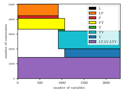
(a) Data set small. Total: 2322 variables, 5033 constraints. Line planning: 6 variables, 9 constraints.

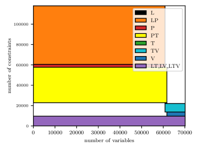
(b) Data set toy. Total: 70152 variables, 118060 constraints. Line planning: 16 variables, 40 constraints.

Figure 7: Matrix structure of the integrated line planning, passenger routing, timetabling and vehicle scheduling problem.

For evaluating the integrated solution approach, we consider different parameters $\lambda_{3},\lambda_{4}$ as weights for the travel time $f_{3}$ and the costs $f_{4}$ in the objective function

$$\lambda_{3}\cdot f_{3}+\lambda_{4}\cdot f_{4}$$

given in Section 3.3. However, for the partially integrated model (LinTimPass), it is often beneficial to include the line costs $f_{1}$ as an approximation of the costs $f_{4}$ and use the auxiliary objective

$$\lambda_{1}\cdot f_{1}+\lambda_{3}\cdot f_{3}.$$

An overview of the parameters used in this section can be found in Table 3.

Data set	$(\lambda_{1},\lambda_{3},\lambda_{4})$	Figure
small	(0, 1000, 1)	8
toy	(0,10,1) (0,1,0) (0,0,1) (0,40,1) (25000,40,-)∗ (25000,10,-)∗ (1000,40,-)∗ (1000,10,-)∗ (500,40,-)∗ (500,10,-)∗	9(a), 10 9(b) 9(c), 10 9(d), 10 10 10 10 10 10 10

Table 3: Parameters used in the objective function. Parameter sets ^∗ are only used for (LinTimPass).

Problem size

As Table 4 shows, the time limit of one hour does not suffice to solve (LinTimPassVeh) to optimality for all considered parameters $\lambda_{3},\lambda_{4}$ for the small artificial data set toy. We therefore compare different partially integrated solution approaches as presented in Figure 4. The solver time of these partially integrated problems is considerably smaller than for (LinTimPassVeh), see Table 4. This is especially obvious for data set toy, where the solver time of the partially integrated problems ranges between 0.003% and 12.2% of the solver time of (LinTimPassVeh). Additionally, Table 4 illustrates the amplification of the increase of the problem size compared to the data set size. While the infrastructure network for data set toy is roughly twice as large as the infrastructure network for data set small, the solver time for (LinTimPassVeh) increases from finding an optimal solution in less than two seconds to an average gap of 50% for the one hour time limit.

Solution approach	small		toy
	time	gap	time	gap
(TimPass)	0.02	0	0.08	0
(LinTimPass)	0.35	0	331.21	0
(TimVeh)	0.52	0	3.42	0
(LinTimPassVeh)	1.35	0	2709.70	50.35%

Table 4: Solver time (in seconds) and optimality gap of the (partially) integrated models for data sets small and toy for a time limit of one hour. The values reported here are mean values over all considered parameters, see Table 3.

Comparing the solution quality of partially integrated solution approaches

In Theorem 14, we show that the integration of the last stages always leads to solution that are better or at least as good as the sequential solution. This is also reflected by the experiments, see Figure 8(a) for data set small and Figure 9 for data set toy. For the latter, we see that emphasizing costs in the objective, which is for $\lambda_{3}=10,\lambda_{4}=1$ or even $\lambda_{3}=0,\lambda_{4}=1$, (TimVeh) leads to a considerable improvement over the sequential solution approach. We marked the solution approaches for which an improvement can be guaranteed with a gray circle.

For the other partially integrated solution approaches, there is no guarantee to find better solutions compared to the sequential approach. Our experiments show that (TimPass) is able to improve the solution quality, see Figures 9(b) to 9(d). However, (LinTimPass) with objective parameters $\lambda_{1}=0,\lambda_{3}>0$ leads to an impaired solution quality for all cases where for the costs $f_{4}$ the parameter is positive, i.e., $\lambda_{4}>0$. Only for the case that only the travel time $f_{3}$ is considered, i.e., for $\lambda_{3}=1,\lambda_{4}=0$, see Figure 9(b), the objective is as good as for (LinTimPassVeh). Note that in this case (LinTimPassVeh) and (LinTimPass) coincide as a feasible vehicle schedule can always be constructed.

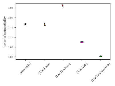
(a) The price of sequentiality.

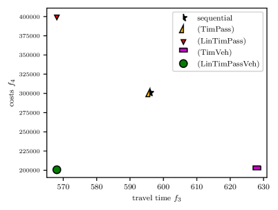
(b) Travel time $f_{3}$ and costs $f_{4}$.

Figure 8: Evaluation of the price of sequentiality as well as of travel time $f_{3}$ and costs $f_{4}$ for data set small for parameters $\lambda_{3}=1000,\lambda_{4}=1$.

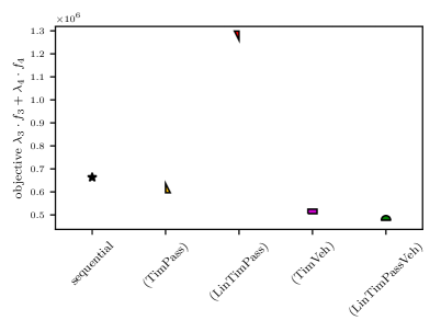
(a) $\lambda_{3}=10,\lambda_{4}=1$

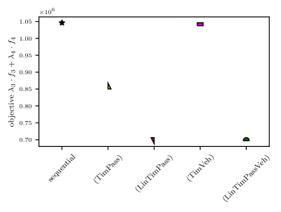
(b) $\lambda_{3}=1,\lambda_{4}=0$

(c) $\lambda_{3}=0,\lambda_{4}=1$

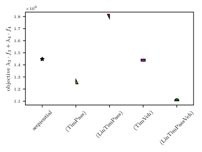
(d) $\lambda_{3}=40,\lambda_{4}=1$

Figure 9: Evaluation of the objective $\lambda_{3}\cdot f_{3}+\lambda_{4}\cdot f_{4}$ for data set toy. We marked the solution approaches for which an improvement can be guaranteed with a gray circle.

Adding auxiliary objectives to the partially integrated solution approaches

Auxiliary objectives in earlier stages of the sequential process and in partially integrated solution approaches may be very helpful. Here, we especially see that using the line costs $f_{1}$ as an approximation of the costs $f_{4}$ significantly improves the solution quality of (LinTimPass). As detailed in Table 3, we changed the objective function for (LinTimPass) from $f_{3}$ to

$$\lambda_{1}\cdot f_{1}+\lambda_{3}\cdot f_{3}$$

for various values of $\lambda_{1},\lambda_{3}$. Figure 10 shows that this enables (LinTimPass) to find solutions with low costs $f_{4}$ in addition to ones with low travel time $f_{3}$.

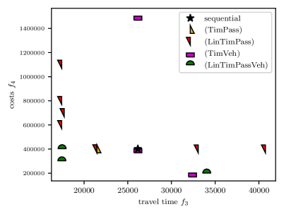
Figure 10: Evaluation of travel time $f_{3}$ and costs $f_{4}$ for different parameter sets $(\lambda_{1},\lambda_{3},\lambda_{4})$ for data set toy, see Table 3. Note that the solutions for (LinTimPassVeh) have not been computed to optimality.

Using varying weighted sum scalarization for finding Pareto solutions

As discussed in Section 2, there exists two possible interpretations of the objective function

$$\lambda_{3}\cdot f_{3}+\lambda_{4}\cdot f_{4}.$$

On the one hand, $\frac{\lambda_{3}}{\lambda_{4}}$ can be regarded as the (known) value of time, such that the objective minimizes the generalized costs. In this case, it suffices to compute solutions for one set of parameters $\lambda_{3},\lambda_{4}$.

On the other hand, we can consider both the travel time $f_{3}$ and the costs $f_{4}$ separately and use multi-objective optimization to find Pareto solutions, i.e., solutions that cannot be improved in both $f_{3}$ and $f_{4}$. Here, the parameter $\lambda_{3},\lambda_{4}$ are scalarization parameters in a weighted sum approach. We consider this in Figures 8(b) and 10. First of all, note that when (LinTimPassVeh) can be computed to optimality, all solutions are weakly Pareto optimal. For data set small, we can even show that the solution for $\lambda_{3}=1000,\lambda_{4}=1$ is an ideal solution. i.e., neither the travel time $f_{3}$ nor the cost $f_{4}$ can be improved. Therefore, we do not need to consider further scalarization parameters for data set small.

For data set toy, the solver time of one hour did not suffice to compute (LinTimPassVeh) to optimality. Therefore, one solution of (LinTimPassVeh) is dominated by a solution of (TimVeh). In regard of the high computation time for (LinTimPassVeh), it is especially interesting to compare the solution quality of the partially integrated solution approaches. As expected, (TimPass) and (LinTimPass) can be used to find solutions with low travel time $f_{3}$ while (TimVeh) finds the solution with the lowest costs $f_{4}$. While the sequential solution approach finds a solution with comparatively low costs $f_{4}$, it is dominated both by solutions of the integrated approach (LinTimPassVeh) and the partially integrated approaches (TimPass) and (LinTimPass). Overall, Figure 10 shows that varying the scalarization parameters lead to interesting compromises between travel time $f_{3}$ and costs $f_{4}$ and that partially integrated solution approaches yield are a good way to generate varying solutions when the expense to solve the integrated problem is too high.

7 Conclusions and further research

In this paper, we consider the integration of sequential problems into a multi-stage problem and compare the solution quality for both approaches by considering the price of sequentiality. While in general the price of sequentiality is unbounded, we show that it highly depends on the definition of the sequential problems and the order in which these are solved. Applying these findings to the sequential problems line planning, timetabling, passenger routing and vehicle scheduling in public transport planning shows that partial integration leads to better solutions than the traditional sequential solution approach while keeping the problem size manageable.

On the one hand, we aim to extend the integrated model for public transportation. For example, the integrated formulation can be extended to include the time slice model introduced in [GGNS16] in order to distribute the favored departure times of the passengers. Another important aspect, especially in high-demand networks is the integration of vehicle capacity for routing as in [BBVL17, GS17, PSS18, YG19]. Both approaches are omitted here to not further complicate the model. Also, the relation to the eigenmodel presented in [Sch17] is under consideration: The different sequential solution approaches of the eigenmodel can be used to retrieve an (equivalent) multi-stage problem for line planning, timetabling, passenger routing and vehicle scheduling that can be compared to the one presented here.

On the other hand, we are working on extending the theoretical background of integrating sequential processes. One important aspect is to incorporate different possibilities to derive objective functions for the multi-stage problem. Here, we are especially considering multi-criteria objective functions, e.g. in the context of complex systems, see [DKK⁺20].

Appendix A IP models for sequential public transport problems

Here we provide details which have been left out in Section 3.2.

A.1 The event-activity network (EAN)

A formal definition of the event-activity network is given. We start with the basic definition needed for timetabling and add the requirements for passenger routing in Notation 18.

Notation 17.

Give a line plan ${\cal L}$, the corresponding event-activity network $\mathcal{N}({\cal L})=(\mathcal{E}({\cal L}),\mathcal{A}({\cal L}))$ is given by arrival and departure events of every line at every stop $\mathcal{E}({\cal L})=\mathcal{E}_{\textup{arr}}({\cal L})\cup\mathcal{E}_{\textup{dep}}({\cal L})$ with

$$\mathcal{E}_{\textup{arr}}({\cal L}) =\{(v,\textup{arr},l)\colon v\in l\cap V,l\in{\cal L}\},$$

$$\mathcal{E}_{\textup{dep}}({\cal L}) =\{(v,\textup{dep},l)\colon v\in l\cap V,l\in{\cal L}\}$$

and drive, wait and transfer activities $\mathcal{A}({\cal L})=\mathcal{A}_{\textup{drive}}({\cal L})\cup\mathcal{A}_{\textup{wait}}({\cal L})\cup\mathcal{A}_{\textup{trans}}({\cal L})$ with

$$\mathcal{A}_{\textup{drive}}({\cal L}) =\{((v_{1},\textup{dep},l),(v_{2},\textup{arr},l))\colon e=(v_{1},v_{2})\in l\cap E,l\in{\cal L}\},$$

$$\mathcal{A}_{\textup{wait}}({\cal L}) =\{((v,\textup{arr},l),(v,\textup{dep},l))\colon v\in l\cap V,l\in{\cal L}\},$$

$$\mathcal{A}_{\textup{trans}}({\cal L}) =\{((v,\textup{arr},l_{1}),(v,\textup{dep},l_{2}))\colon v\in l_{1}\cap l_{2}\cap V,l_{1},l_{2}\in{\cal L},l_{1}\neq l_{2}\}.$$

For a simpler notation, we collect the drive and wait activities of line $l$ in $\mathcal{A}(l)$ and the transfer activities between line $l_{1}$ and $l_{2}$ in $\mathcal{A}(l_{1},l_{2})$.

Finally, for each activity $a\in\mathcal{A}({\cal L})$, upper and lower bounds on the duration of the activity are given as $L_{a},U_{a}\in\mathbb{N}$ with $0\leq L_{a}\leq U_{a}$. We define these lower and upper bounds of the activities according to the edges of the underlying PTN. More precisely, we assume that in the PTN lower and upper bounds $L_{e}^{\textup{drive}}\leq U_{e}^{\textup{drive}}$ for travel along edge $e\in E$ are given and that $L_{v}^{\textup{wait}}\leq U_{v}^{\textup{wait}}$, $L_{v}^{\textup{trans}}\leq U_{v}^{\textup{trans}}$, $v\in V$, are the stop dependent bounds for the dwell times of a vehicle and for the transfer time of a passenger. We set:

$$L_{a} =L_{e}^{\textup{drive}}, U_{a} =U_{e}^{\textup{drive}}, \quad a=((u,l,\textup{dep}),(v,l,\textup{arr}))\in\mathcal{A}_{\textup{drive}}({\cal L}),e=(u,v)$$

$$L_{a} =L_{v}^{\textup{wait}}, U_{a} =U_{v}^{\textup{wait}}, \quad a=((v,l,\textup{arr}),(v,l,\textup{dep}))\in\mathcal{A}_{\textup{wait}}({\cal L})$$ (11)

$$L_{a} =L_{v}^{\textup{trans}}, U_{a} =U_{v}^{\textup{trans}}, \quad a=((v,l_{1},\textup{arr}),(v,l_{2},\textup{dep}))\in\mathcal{A}_{\textup{trans}}({\cal L})$$

To correctly model the passenger routing, the EAN has to be extended. Therefore, we include auxiliary events representing source and target nodes for all OD pairs as well as activities connecting these auxiliary events to the rest of the EAN. Along the lines of [Sch14], we receive:

Notation 18.

Given an event-activity network $\mathcal{N}({\cal L})=(\mathcal{E}({\cal L}),\mathcal{A}({\cal L}))$, the extended event-activity network $\bar{\mathcal{N}}({\cal L})=(\bar{\mathcal{E}}({\cal L}),\bar{\mathcal{A}}({\cal L}))$ is the following extension of $\mathcal{N}({\cal L})$: $\bar{\mathcal{E}}({\cal L})=\mathcal{E}({\cal L})\cup\mathcal{E}_{\textup{aux}}({\cal L})$, $\bar{\mathcal{A}}({\cal L})=\mathcal{A}({\cal L})\cup\mathcal{A}({\cal L})_{\textup{aux}}$ with

$$\mathcal{E}_{\textup{aux}}({\cal L}) =\{(v,\textup{source}),(v,\textup{target})\colon v\in V\}$$

$$\mathcal{A}_{\textup{aux}}({\cal L}) =\{((v,\textup{source}),(v,l,\textup{dep}))\colon v\in l\cap V,l\in{\cal L}\}$$

$$\qquad\cup\{((v,l,\textup{arr}),(v,\textup{target}))\colon v\in l\cap V,l\in{\cal L}\}.$$

For the auxiliary activities $a\in\mathcal{A}_{\textup{aux}}({\cal L})$ we set $L_{a}=U_{a}=0$.

A.2 Passenger routing (Pass)

Using the node-arc-incidence matrix $A({\cal L})$ of $\bar{\mathcal{N}}({\cal L})$, binary variables $p_{a}^{u,v}$ for determining whether activity $a\in\mathcal{A}({\cal L})$ is part of a $u-v$ path and vector $b^{u,v}$ with

$$b^{u,v}_{i}=\begin{cases}1,&\textup{if }i=(u,\textup{source})\\ -1,&\textup{if }i=(v,\textup{target})\\ 0,&\textup{otherwise}\end{cases}$$

we get the following flow formulation for finding a passenger routing.

$$\min\sum_{(u,v)\in\textup{OD}}\sum_{a\in\mathcal{A}({\cal L})} p_{a}^{u,v}\cdot L_{a}$$

$$\textup{s.t.}\quad A({\cal L})\cdot(p^{u,v}) =b^{u,v} \qquad(u,v)\in\textup{OD}$$

$$p_{a}^{u,v} \in\{0,1\} \qquad a\in\bar{\mathcal{A}}({\cal L}),(u,v)\in\textup{OD}$$

A.3 Timetabling (Tim)

The classical integer programming model for periodic timetabling uses the so-called modulo parameters $z_{a}\in\mathbb{Z}$ for all $a\in\mathcal{A}({\cal L})$ to model the periodicity of the timetable. As input, one needs the event-activity network $\mathcal{N}({\cal L})$ (which depends on stage 1) and the number of passengers $w_{a}(\bar{p})$ which use activity $a\in\mathcal{A}({\cal L})$. These numbers depend on the paths computed in stage 2.

$$\min\sum_{a\in\mathcal{A}({\cal L})}w_{a}(\bar{p})\cdot(\pi_{j} -\pi_{i}+z_{a}\cdot T)$$

$$\textup{s.t.}\quad\pi_{j}-\pi_{i}+z_{a}\cdot T \geq L_{a}\qquad a=(i,j)\in\mathcal{A}({\cal L})$$ (12)

$$\pi_{j}-\pi_{i}+z_{a}\cdot T \leq U_{a} a=(i,j)\in\mathcal{A}({\cal L})$$

$$\pi_{i} \in\{0,\ldots,T-1\}\quad i\in\mathcal{E}({\cal L})$$

$$z_{a} \in\mathbb{Z} a\in\mathcal{A}({\cal L})$$

Linearization of (10):

$$\eta_{a} =\bar{y}_{l_{1}}\cdot\bar{y}_{l_{2}} a\in\mathcal{A}(l_{1},l_{2})$$

can be linearized to

$$\eta_{a} \leq\bar{y}_{l_{1}} a\in\mathcal{A}(l_{1},l_{2})$$ (13)

$$\eta_{a} \leq\bar{y}_{l_{2}} a\in\mathcal{A}(l_{1},l_{2})$$ (14)

$$\eta_{a} \geq\bar{y}_{l_{1}}+\bar{y}_{l_{2}}-1 a\in\mathcal{A}(l_{1},l_{2}).$$ (15)

A.4 Vehicle scheduling (Veh)

A trip $\tau=(t,l)$ is determined by the line $l\in{\cal L}$ that is covered and the period $t\in\mathcal{T}$ in which the trip starts. It has to be operated by one vehicle end-to-end. We use boolean variables $x_{(t_{1},l_{1}),(t_{2},l_{2})}$ to indicate if trip $(t_{2},l_{2})$ is operated by the vehicle that directly before that operated trip $(t_{1},l_{1})$ and boolean variables $x_{\textup{depot},(t,l)}$, $x_{(t,l),\textup{depot}}$ to indicate if trip $(t,l)$ is the first or last trip in a vehicle route operated from or to the depot. If $x_{(t_{1},l_{1}),(t_{2},l_{2})}=1$, the difference between the end time $\omega_{t_{1},l_{1}}$ of trip $(t_{1},l_{1})$ and the start time $\alpha_{t_{2},l_{2}}$ of trip $(t_{2},l_{2})$ has to be at least $L_{l_{1},l_{2}}$. We get the following IP formulation for the vehicle scheduling problem.

$$\min\textup{cost}(\textup{Veh})\qquad\qquad\qquad\qquad$$

$$\textup{s.t.}\quad x_{(t_{1},l_{1}),(t_{2},l_{2})}\cdot L_{l_{1},l_{2}} \leq\alpha_{t_{2},l_{2}}-\omega_{t_{1},l_{1}}\quad t_{1},t_{2}\in\mathcal{T},l_{1},l_{2}\in{\cal L}$$

$$\sum_{t_{1}\in\mathcal{T}}\sum_{l_{1}\in{\cal L}}x_{(t_{1},l_{1}),(t_{2},l_{2})}+x_{\textup{depot},(t_{2},l_{2})} =1\quad t_{2}\in\mathcal{T},l_{2}\in{\cal L}$$ (16)

$$\sum_{t_{2}\in\mathcal{T}}\sum_{l_{2}\in{\cal L}}x_{(t_{1},l_{1}),(t_{2},l_{2})}+x_{(t_{1},l_{1}),\textup{depot}} =1\quad t_{1}\in\mathcal{T},l_{1}\in{\cal L}$$

$$x_{(t_{1},l_{1}),(t_{2},l_{2})} \in\{0,1\} t_{1},t_{2}\in\mathcal{T},l_{1},l_{2}\in{\cal L}$$

$$x_{\textup{depot},(t,l)},x_{(t,l),\textup{depot}} \in\{0,1\} p\in\mathcal{T},l\in{\cal L}$$

Depending on stages 1 to 3, the vehicle scheduling problem can be formulated as follows. Note that while the start and end times $\alpha_{t,l}$, $\omega_{t,l}$ of trips $(t,l)$, $t\in\mathcal{T},l\in{\cal L}^{0}$, as well as the duration of a trip on line $l$ $\delta_{l}$ are now variables, their values can be predetermined as they only depend on fixed variables $\pi,z$.

The objective function $f_{4}(\bar{y},\bar{p},\bar{\pi},\bar{z};x)$ represents the costs $\textup{cost}(\textup{Veh})$ of vehicle schedule Veh. They depend on the duration and distance covered by the vehicles as well as the number of vehicles needed. We distinguish between the time and distance needed for trips, i.e., when passengers may be on board, and the time and distance needed for so-called empty (or deadheading) trips when no passengers may be on board. These empty trips include time between two consecutive trips in a vehicle route, the distance of potential relocation (or deadheading) trips as well as trips to and from the depot at the end and the start of a vehicle route, respectively. The details are listed in Table 5.

$$\min\quad f_{4}(\bar{y},\bar{p},\bar{\pi},\bar{z};x)=$$

$$\gamma_{1}\cdot\sum_{l\in{\cal L}^{0}}\bar{y}_{l}\cdot\delta_{l}$$ (17)

$$+\gamma_{2}\cdot\sum_{l\in{\cal L}^{0}}\bar{y}_{l}\cdot\textup{length}_{l}$$ (18)

$$+\gamma_{3}\cdot\sum_{t_{1}\in\mathcal{T}}\sum_{l_{1}\in{\cal L}^{0}}\Big{(}\sum_{t_{2}\in\mathcal{T}}\sum_{l_{2}\in{\cal L}^{0}}\big{(}\alpha_{(t_{2},l_{2})}-\omega_{(t_{1},l_{1})}\big{)}\cdot x_{(t_{1},l_{2}),(t_{2},l_{2})}$$

$$\qquad\qquad\qquad+x_{\textup{depot},(t_{1},l_{1})}\cdot L_{\textup{depot},l_{1}}+x_{(t_{1},l_{1}),\textup{depot}}\cdot L_{l_{1},\textup{depot}}\Big{)}$$ (19)

$$+\gamma_{4}\cdot\sum_{t_{1}\in\mathcal{T}}\sum_{l_{1}\in{\cal L}^{0}}\Big{(}\sum_{t_{2}\in\mathcal{T}}\sum_{l_{2}\in{\cal L}^{0}}\big{(}x_{(t_{1},l_{1}),(t_{2},l_{2})}\cdot D_{l_{1},l_{2}}\big{)}$$

$$\qquad\qquad\qquad+x_{\textup{dep},(t_{1},l_{1})}\cdot D_{\textup{dep},l_{1}}+x_{(t_{1},l_{1}),\textup{dep}}\cdot D_{l_{1},\textup{dep}}\Big{)}$$ (20)

$$+\gamma_{5}\cdot\sum_{t\in\mathcal{T}}\sum_{l\in{\cal L}^{0}}x_{\textup{depot},(t,l)}$$ (21)

s.t. $$\delta_{l} =\sum_{a=(i,j)\in\mathcal{A}(l)}(\bar{\pi}_{j}-\bar{\pi}_{i}+\bar{z}_{a}\cdot T)\;\; l\in{\cal L}^{0}$$ (22)

$$\alpha_{t,l} =t\cdot T+\bar{\pi}_{\texttt{first}(l)} t\in\mathcal{T},l\in{\cal L}^{0}$$ (23)

$$\omega_{t,l} =t\cdot T+\bar{\pi}_{\texttt{first}(l)}+\delta_{l} t\in\mathcal{T},l\in{\cal L}^{0}$$ (24)

$$\alpha_{t_{2},l_{2}}-\omega_{t_{1},l_{1}} \geq x_{(t_{1},l_{1}),(t_{2},l_{2})}\cdot L_{l_{1},l_{2}}$$

$$\quad-M^{\prime}\cdot(1-x_{(t_{1},l_{1}),(t_{2},l_{2})})\quad t_{1},t_{2}\in\mathcal{T},l_{1},l_{2}\in{\cal L}^{0}$$ (25)

$$\bar{y}_{l_{2}} =\sum_{t_{1}\in\mathcal{T}}\sum_{l_{1}\in{\cal L}^{0}}x_{(t_{1},l_{1}),(t_{2},l_{2})}$$

$$\quad+x_{\textup{depot},(t_{2},l_{2})} t_{2}\in\mathcal{T},l_{2}\in{\cal L}^{0}$$ (26)

$$\bar{y}_{l_{1}} =\sum_{t_{2}\in\mathcal{T}}\sum_{l_{2}\in{\cal L}^{0}}x_{(t_{1},l_{1}),(t_{2},l_{2})}$$

$$\quad+x_{(t_{1},l_{1}),\textup{depot}} t_{1}\in\mathcal{T},l_{1}\in{\cal L}^{0}$$ (27)

$$x_{(t,l),\bullet} \leq\bar{y}_{l} t\in\mathcal{T},l\in{\cal L}^{0}$$ (28)

$$x_{\bullet,(t,l)} \leq\bar{y}_{l} t\in\mathcal{T},l\in{\cal L}^{0}$$ (29)

$$\delta_{l},\alpha_{t,l},\omega_{t,l} \in\mathbb{N},$$ (30)

$$x_{(t_{1},l_{1}),(t_{2},l_{2})},x_{\textup{depot},(t,l)},x_{(t,l),\textup{depot}} \in\{0,1\}$$ (31)

Cost type		Weighting factor	Components
time based trip costs	(17)	$\gamma_{1}$	$\delta_{l}$ duration of a trip on line $l$
distance based trip costs	(18)	$\gamma_{2}$	$\textup{length}_{l}$ length of a trip on line $l$
time based empty trip costs	(19)	$\gamma_{3}$	$\alpha_{(t_{2},l_{2})}-\omega_{(t_{1},l_{1})}$ duration of empty trip $L_{\textup{depot},l}$ time from depot to start of line $l$ $L_{l,\textup{depot}}$ time from end of line $l$ to depot
distance based empty trip costs	(20)	$\gamma_{4}$	$D_{l_{1},l_{2}}$ length of empty trip $D_{\textup{depot},l}$ distance from depot to start of line $l$ $D_{l,\textup{depot}}$ distance from end of line $l$ to depot
vehicle based costs	(21)	$\gamma_{5}$	number of vehicles

Table 5: All parts of the objective function considered in vehicle scheduling.

In constraints (22), (23) and (24), the duration of a trip on line $l$ as well as the start and end time of trip $(t,l)$, $t\in\mathcal{T},l\in{\cal L}^{0}$, are computed. Note that the variables $\bar{\pi},\bar{z}$ are already fixed and that $\texttt{first}(l)$, $l\in{\cal L}^{0}$, represents the first event in line $l$. Constraint (25) ensures that the time between the start and end of consecutive trips is sufficiently long while constraints (26) to (29) model the vehicle flow for all operated lines.

References

- [AADP+18] N. Absi, C. Archetti, S. Dauzère-Pérès, D. Feillet, and M.G. Speranza. Comparing sequential and integrated approaches for the production routing problem. European Journal of Operational Research, 269(2):633–646, 2018.
- [AS16] C. Archetti and M.G. Speranza. The inventory routing problem: the value of integration. International Transactions in Operational Research, 23(3):393–407, 2016.
- [BBVL17] S. Burggraeve, S. Bull, P. Vansteenwegen, and R. Lusby. Integrating robust timetabling in line plan optimization for railway systems. Transportation Research Part C: Emerging Technologies, 77:134–160, 2017.
- [BCHP20] V. Blanco, E. Conde, Y. Hinojosa, and J. Puerto. An optimization model for line planning and timetabling in automated urban metro subway networks. a case study. Omega, 92:102165, 2020.
- [BGP07] R. Borndörfer, M. Grötschel, and M.E. Pfetsch. A column generation approach to line planning in public transport. Transportation Science, 41:123–132, 2007.
- [BHK17] R. Borndörfer, H. Hoppmann, and M. Karbstein. Passenger routing for periodic timetable optimization. Public Transport, 9(1-2):115–135, 2017.
- [BHKL20] R. Borndörfer, H. Hoppmann, M. Karbstein, and N. Lindner. Separation of cycle inequalities in periodic timetabling. Discrete Optimization, 35, 2020.
- [BK09] S. Bunte and N. Kliewer. An overview on vehicle scheduling models. Public Transport, 1(4):299–317, 2009.
- [BKLL18] R. Borndörfer, M. Karbstein, C. Liebchen, and N. Lindner. A Simple Way to Compute the Number of Vehicles That Are Required to Operate a Periodic Timetable. In 18th Workshop on Algorithmic Approaches for Transportation Modelling, Optimization, and Systems (ATMOS 2018), volume 65 of OpenAccess Series in Informatics (OASIcs), pages 16:1–16:15, 2018.
- [BLR19] R. Borndörfer, N. Lindner, and S. Roth. A concurrent approach to the periodic event scheduling problem. Journal of Rail Transport Planning & Management, page 100175, 2019.
- [BSS20] P. Bouman, A. Schiewe, and P. Schiewe. A New Sequential Approach to Periodic Vehicle Scheduling and Timetabling. In 20th Symposium on Algorithmic Approaches for Transportation Modelling, Optimization, and Systems (ATMOS 2020), volume 85 of OpenAccess Series in Informatics (OASIcs), pages 6:1–6:16, 2020.
- [BWZ97] M. Bussieck, T. Winter, and U. Zimmermann. Discrete optimization in public rail transport. Mathematical programming, 79(1-3):415–444, 1997.
- [CFG+19] S. Carosi, A. Frangioni, L. Galli, L. Girardi, and G. Vallese. A matheuristic for integrated timetabling and vehicle scheduling. Transportation Research Part B: Methodological, 127:99 – 124, 2019.
- [CW86] A. Ceder and N.H.M. Wilson. Bus network design. Transportation Research B, 20(4):331–344, 1986.
- [DC18] M. Darvish and L. C. Coelho. Sequential versus integrated optimization: Production, location, inventory control, and distribution. European Journal of Operational Research, 268(1):203 – 214, 2018.
- [DH07] G. Desaulniers and M. Hickman. Public transit. Handbooks in operations research and management science, 14:69–127, 2007.
- [DKK+20] T. Dietz, K. Klamroth, K. Kraus, S. Ruzika, L. E. Schäfer, B. Schulze, M. Stiglmayr, and M. M. Wiecek. Introducing multiobjective complex systems. European Journal of Operational Research, 280(2):581–596, 2020.
- [DRB+17] S. Dutta, N. Rangaraj, M. Belur, S. Dangayach, and K. Singh. Construction of periodic timetables on a suburban rail network-case study from Mumbai. In RailLille 2017—7th International Conference on Railway Operations Modelling and Analysis, 2017.
- [Ehr05] M. Ehrgott. Multicriteria Optimization. Springer, Berlin, Heidelberg, 2005.
- [FHSS18] M. Friedrich, M. Hartl, A. Schiewe, and A. Schöbel. System Headways in Line Planning. In Proceedings of CASPT 2018, 2018.
- [FvdHRL18] J. Fonseca, E. van der Hurk, R. Roberti, and A. Larsen. A matheuristic for transfer synchronization through integrated timetabling and vehicle scheduling. Transportation Research Part B: Methodological, 109:128–149, 2018.
- [GBV+19] P. C. Guedes, D. Borenstein, M.S. Visentini, O. C. Bassi de Araújo, and A. F. Kummer Neto. Vehicle scheduling problem with loss in bus ridership. Computers & Operations Research, 111:230 – 242, 2019.
- [GGNS16] P. Gattermann, P. Großmann, K. Nachtigall, and A. Schöbel. Integrating Passengers’ Routes in Periodic Timetabling: A SAT approach. In 16th Workshop on Algorithmic Approaches for Transportation Modelling, Optimization, and Systems (ATMOS 2016), volume 54 of OpenAccess Series in Informatics (OASIcs), pages 1–15, 2016.
- [GH10] V. Guihaire and J.-K. Hao. Transit network timetabling and vehicle assignment for regulating authorities. Computers & Industrial Engineering, 59(1):16–23, 2010.
- [GS17] M. Goerigk and M. Schmidt. Line planning with user-optimal route choice. European Journal of Operational Research, 259(2):424–436, 2017.
- [GS18] L. Galli and S. Stiller. Modern challenges in timetabling. In Handbook of Optimization in the Railway Industry, pages 117–140. Springer, 2018.
- [GSYG20] Y. Gao, M. Schmidt, L. Yang, and Z. Gao. A branch-and-price approach for trip sequence planning of high-speed train units. Omega, 92:102150, 2020.
- [Gur18] Gurobi Optimizer. http://www.gurobi.com/, 2018. Gurobi Optimizer Version 8.0, Houston, Texas: Gurobi Optimization, Inc.
- [HDD01] K. Haase, G. Desaulniers, and J. Desrosiers. Simultaneous vehicle and crew scheduling in urban mass transit systems. Transportation Science, 35(3):286–303, 2001.
- [JS20] S. Jäger and A. Schöbel. The blockwise coordinate descent method for integer programs. Mathematical Methods of Operations Research, 91:357–381, 2020.
- [KDC18] M. Kidd, M. Darvish, and L. Coelho. On the value of integration in supply chain planning. In 29th European Conference on Operational Research (EURO 2018), 2018.
- [KMN+20] K. Klamroth, S. Mostaghim, B. Naujoks, S. Poles, R. Purshouse, G. Rudolph, S. Ruzika, S. Sayin, M.M. Wiecek, and X. Yao. Multiobjective optimization for interwoven systems. Journal of Multi-Criteria Decision Analysis, 24(1-2):71–81, 2020.
- [KR13] M. Kaspi and T. Raviv. Service-oriented line planning and timetabling for passenger trains. Transportation Science, 47(3):295–311, 2013.
- [LdlCS21] N. Lindner, P. Maristany de las Casas, and P. Schiewe. Optimal Forks: Preprocessing Single-Source Shortest Path Instances with Interval Data. In 21st Workshop on Algorithmic Approaches for Transportation Modelling, Optimization, and Systems (ATMOS 2021), 2021.
- [LHS18] K. Li, H. Huang, and P. Schonfeld. Metro timetabling for time-varying passenger demand and congestion at stations. Journal of Advanced Transportation, 2018.
- [Lie06] C. Liebchen. Periodic Timetable Optimization in Public Transport. dissertation.de – Verlag im Internet, Berlin, 2006.
- [Lie08] C. Liebchen. Linien-, Fahrplan-, Umlauf-und Dienstplanoptimierung: Wie weit können diese bereits integriert werden? In Heureka’08, 2008.
- [Lin00] T. Lindner. Train schedule optimization in public rail transport. PhD thesis, Technische Universität Braunschweig, 2000.
- [LLB18] R.M. Lusby, J. Larsen, and S. Bull. A survey on robustness in railway planning. European Journal of Operational Research, 266:1–15, 2018.
- [LP15] M.E. Lübbecke and C. Puchert. Primal heuristics for mixed integer programs with a staircase structure. Technical report, RWTH Aachen, 2015.
- [LPSS18] M.E. Lübbecke, C. Puchert, P. Schiewe, and A. Schöbel. Integrating line planning, timetabling and vehicle scheduling - Integer programming formulation and analysis. In Proceedings of CASPT 2018, 2018.
- [MS09] M. Michaelis and A. Schöbel. Integrating line planning, timetabling, and vehicle scheduling: A customer-oriented approach. Public Transport, 1(3):211–232, 2009.
- [Nac98] K. Nachtigall. Periodic Network Optimization and Fixed Interval Timetables. PhD thesis, University of Hildesheim, 1998.
- [PLM+13] H. Petersen, A. Larsen, O. Madsen, B. Petersen, and S. Ropke. The simultaneous vehicle scheduling and passenger service problem. Transportation Science, 47(4):603–616, 2013.
- [PSH21] G.-J. Polinder, M. Schmidt, and D. Huisman. Timetabling for strategic passenger railway planning. Transportation Research Part B: Methodological, 146:111–135, 2021.
- [PSS18] J. Pätzold, A. Schiewe, and A. Schöbel. Cost-minimal public transport planning. In 18th Workshop on Algorithmic Approaches for Transportation Modelling, Optimization, and Systems (ATMOS 2018), volume 65 of OpenAccess Series in Informatics (OASIcs), pages 8:1–8:22, 2018.
- [PSSS17] J. Pätzold, A. Schiewe, P. Schiewe, and A. Schöbel. Look-Ahead Approaches for Integrated Planning in Public Transportation. In 17th Workshop on Algorithmic Approaches for Transportation Modelling, Optimization, and Systems (ATMOS 2017), volume 59 of OpenAccess Series in Informatics (OASIcs), pages 1–16, 2017.
- [RN09] M. Rittner and K. Nachtigall. Simultane Liniennetz- und Fahrlagenoptimierung. Der Eisenbahningenieur, 2009.
- [RSAMB17] T. Robenek, S. Sharif Azadeh, Y. Maknoon, and M. Bierlaire. Hybrid cyclicity: Combining the benefits of cyclic and non-cyclic timetables. Transportation Research Part C: Emerging Technologies, 75:228–253, 2017.
- [ŞABS20] G. Şahin, A. Ahmadi Digehsara, R. Borndörfer, and T. Schlechte. Multi-period line planning with resource transfers. Transportation Research Part C: Emerging Technologies, 119:102726, 2020.
- [SAS+] A. Schiewe, S. Albert, P. Schiewe, A. Schöbel, and F. Spühler. LinTim - Integrated Optimization in Public Transportation. Homepage. https://www.lintim.net/. open source.
- [SAS+20] A. Schiewe, S. Albert, P. Schiewe, A. Schöbel, and F. Spühler. LinTim: An integrated environment for mathematical public transport optimization. Documentation for LinTim 2020.12. Technical report, TU Kaiserslautern, Fachbereich Mathematik, 2020.
- [Sch12] A. Schöbel. Line planning in public transportation: models and methods. OR Spectrum, 34(3):491–510, 2012.
- [Sch14] M. Schmidt. Integrating Routing Decisions in Public Transportation Problems, volume 89 of Optimization and Its Applications. Springer, 2014.
- [Sch17] A. Schöbel. An eigenmodel for iterative line planning, timetabling and vehicle scheduling in public transportation. Transportation Research C, 74:348–365, 2017.
- [Sch20] P. Schiewe. Integrated Optimization in Public Transport Planning, volume 160 of Optimization and Its Applications. Springer, 2020.
- [SE15] V. Schmid and J. Ehmke. Integrated timetabling and vehicle scheduling with balanced departure times. OR Spectrum, 37(4):903–928, 2015.
- [SG13] M. Siebert and M. Goerigk. An experimental comparison of periodic timetabling models. Computers & Operations Research, 40(10):2251–2259, 2013.
- [SS06] A. Schöbel and S. Scholl. Line planning with minimal travel time. In 5th Workshop on Algorithmic Methods and Models for Optimization of Railways, number 06901 in Dagstuhl Seminar Proceedings, 2006.
- [SS10] M. Schmidt and A. Schöbel. The complexity of integrating routing decisions in public transportation models. In Proceedings of ATMOS10, volume 14 of OpenAccess Series in Informatics (OASIcs), pages 156–169, 2010.
- [SS15] M. Schmidt and A. Schöbel. The complexity of integrating routing decisions in public transportation models. Networks, 65(3):228–243, 2015.
- [SS20] P. Schiewe and A. Schöbel. Periodic timetabling with integrated routing: Toward applicable approaches. Transportation Science, 54(6):1714–1731, 2020.
- [SSR20] P. Schiewe, A. Schöbel, and S. Ruzika. Kosten oder Reisezeit? Bikriterielle Optimierung der integrierten Fahr- und Umlaufplanung. In Preprint Heureka’21. Forschungsgesellschaft für Straßen- und Verkehrswesen (FGSV) e.V., 2020.
- [SSS19] A. Schiewe, P. Schiewe, and M. Schmidt. The line planning routing game. European Journal of Operational Research, 274(2):560 – 573, 2019.
- [vL21] R. N. van Lieshout. Integrated periodic timetabling and vehicle circulation scheduling. Transportation Science, 55(3):768–790, 2021.
- [YG19] F. Yan and R. M.P. Goverde. Combined line planning and train timetabling for strongly heterogeneous railway lines with direct connections. Transportation Research Part B: Methodological, 127:20 – 46, 2019.
- [YHWL17] Y. Yue, J. Han, S. Wang, and X. Liu. Integrated train timetabling and rolling stock scheduling model based on time-dependent demand for urban rail transit. Computer-Aided Civil and Infrastructure Engineering, 32(10):856–873, 2017.