A Variability Fault Localization Approach for Software Product Lines

Abstract

Software fault localization is one of the most expensive, tedious, and time-consuming activities in program debugging. This activity becomes even much more challenging in Software Product Line (SPL) systems due to variability of failures. These unexpected behaviors are induced by variability faults which can only be exposed under some combinations of system features. The interaction among these features causes the failures of the system. Although localizing bugs in single-system engineering has been studied in-depth, variability fault localization in SPL systems still remains mostly unexplored. In this article, we present VarCop, a novel and effective variability fault localization approach. For an SPL system failed by variability bugs, VarCop isolates suspicious code statements by analyzing the overall test results of the sampled products and their source code. The isolated suspicious statements are the statements related to the interaction among the features which are necessary for the visibility of the bugs in the system. In VarCop, the suspiciousness of each isolated statement is assessed based on both the overall test results of the products containing the statement as well as the detailed results of the test cases executed by the statement in these products. On a large public dataset of buggy SPL systems, our empirical evaluation shows that VarCop significantly improves two state-of-the-art techniques by 33% and 50% in ranking the incorrect statements in the systems containing a single bug each. In about two-thirds of the cases, VarCop correctly ranks the buggy statements at the top-3 positions in the ranked lists. For the cases containing multiple bugs, VarCop outperforms the state-of-the-art approaches 2 times and 10 times in the proportion of bugs localized at the top-1 positions. Especially, in 22% and 65% of the buggy versions, VarCop correctly ranks at least one bug in a system at the top-1 and top-5 positions.

1 Introduction

Many software projects enable developers to configure to different environments and requirements. In practice, a project adopting the Software Product Line (SPL) methodology [1] can tailor its functional and nonfunctional properties to the requirements of users [1, 2]. This has been done using a very large number of options which are used to control different features [2] additional to the core software. A set of selections of all the features (configurations) defines a program variant (product). For example, Linux Kernel supports thousands of features controlled by +12K compile-time options, that can be configured to generate specific kernel variants for billions of possible scenarios.

However, the variability that is inherent to SPL systems challenges quality assurance (QA) [3, 4, 5, 6, 7]. In comparison with the single-system engineering, fault detection and localization through testing in SPL systems are more problematic, as a bug can be variable (so-called variability bug), which can only be exposed under some combinations of the system features [3, 8]. Specially, there exists a set of the features that must be selected to be on and off together to necessarily reveal the bug. Due to the presence/absence of the interaction among the features in such set, the buggy statements behave differently in the products where these features are on and off together or not. Hence, the incorrect statements can only expose their bugginess in some particular products, yet cannot in the others. Specially, in an SPL system, variability bugs only cause failures in certain products, and the others still pass all their tests. This variability property causes considerable difficulties for localizing this kind of bugs in SPL systems. In the rest of this paper, variability bugs are our focus, and we simply call a system containing variability bugs a buggy (SPL) system.

Despite the importance of variability fault localization, the existing fault localization (FL) approaches [9, 10, 11] are not designed for this kind of bugs. These techniques are specialized for finding bugs in a particular product. For instance, to isolate the bugs causing failures in multiple products of a single SPL system, the slice-based methods [12, 13, 9] could be used to identify all the failure-related slices for each product independently of others. Consequently, there are multiple sets of large numbers of isolated statements that need to be examined to find the bugs. This makes the slice-based methods [9] become impractical in SPL systems.

In addition, the state-of-the-art technique, Spectrum-Based Fault Localization (SBFL) [11, 14, 15, 16, 17] can be used to calculate the suspiciousness scores of code statements based on the test information (i.e., program spectra) of each product of the system separately. For each product, it produces a ranked list of suspicious statements. As a result, there might be multiple ranked lists produced for a single SPL system which is failed by variability bugs. From these multiple lists, developers cannot determine a starting point to diagnose the root causes of the failures. Hence, it is inefficient to find variability bugs by using SBFL to rank suspicious statements in multiple variants separately.

Another method to apply SBFL for localizing variability bugs in an SPL system is that one can treat the whole system as a single program [18]. This means that the mechanism controlling the presence/absence of the features in the system (e.g., the preprocessor directives #ifdef) would be considered as the corresponding conditional if-then statements during the localization process. By this adaptation of SBFL, a single ranked list of the statements for variability bugs can be produced according to the suspiciousness score of each statement. Note that, we consider the product-based testing [19, 20]. Specially, each product is considered to be tested individually with its own test set. Additionally, a test, which is designed to test a feature in domain engineering, is concretized to multiple test cases according to products’ requirements in application engineering [19]. Using this adaptation, the suspiciousness score of the statement is measured based on the total numbers of the passed and failed tests executed by it in all the tested products. Meanwhile, the characteristics including the interactions between system features and the variability of failures among products are also useful to isolate and localize variability bugs in SPL systems. However, these kinds of important information are not utilized in the existing approaches.

In this paper, we propose VarCop, a novel fault localization approach for variability bugs. Our key ideas in VarCop is that variability bugs are localized based on (i) the interaction among the features which are necessary to reveal the bugs, and (ii) the bugginess exposure which is reflected via both the overall test results of products and the detailed result of each test case in the products.

Particularly, for a buggy SPL system, VarCop detects sets of the features which need to be selected on/off together to make the system fail by analyzing the overall test results (i.e., the state of passing all tests or failing at least one test) of the products. We call each of these sets of the feature selections a Buggy Partial Configuration (Buggy PC). Then, VarCop analyzes the interaction among the features in these Buggy PCs to isolate the statements which are suspicious. In VarCop, the suspiciousness of each isolated statement is assessed based on two criteria. The first criterion is based on the overall test results of the products containing the statement. By this criterion, the more failing products and the fewer passing products where the statement appears, the more suspicious the statement is. Meanwhile, the second one is assessed based on the suspiciousness of the statement in the failing products which contain it. Specially, in each failing product, the statement’s suspiciousness is measured based on the detailed results of the products’ test cases. The idea is that if the statement is more suspicious in the failing products based on their detailed test results, the statement is also more likely to be buggy in the whole system.

We conducted experiments to evaluate VarCop in both single-bug and multiple-bug settings on a dataset of 1,570 versions (cases) containing variability bug(s) [18]. We compared VarCop with the state-of-the-art approaches including (SBFL) [11, 14, 15, 16, 17], the combination of the slicing method and SBFL (S-SBFL) [21, 22], and Arrieta et al. [10] using 30 most popular SBFL ranking metrics [14, 15, 11].

For the cases containing a single incorrect statement (single-bug), our results show that VarCop significantly outperformed S-SBFL, SBFL, and Arrieta et al. [10] in all 30/30 metrics by 33%, 50%, and 95% in Rank, respectively. Impressively, VarCop correctly ranked the bugs at the top-3 positions in +65% of the cases. In addition, VarCop effectively ranked the buggy statements first in about 30% of the cases, which doubles the corresponding figure of SBFL.

For localizing multiple incorrect statements (multiple-bug), after inspecting the first statement in the ranked list resulted by VarCop, up to 10% of the bugs in a system can be found, which is 2 times and 10 times better than S-SBFL and SBFL, respectively. Especially, our results also show that in 22% and 65% of the cases, VarCop effectively localized at least one buggy statement of a system at top-1 and top-5 positions. From that, developers can iterate the process of bugs detecting, bugs fixing, and regression testing to quickly fix all the bugs and assure the quality of SPL systems.

In brief, this paper makes the following contributions:

1. A formulation of Buggy Partial Configuration (Buggy PC) where the interaction among the features in the Buggy PC is the root cause of the failures caused by variability bugs in SPL systems.

2. VarCop: A novel effective approach/tool to localize variability bugs in SPL systems.

3. An extensive experimental evaluation showing the performance of VarCop over the state-of-the-art methods.

2 Motivating Example

In this section, we illustrate the challenges of localizing variability bugs and motivate our solution via an example.

2.1 An Example of Variability Bugs in SPL Systems

⬇

1int maxWeight = 2000, weight = 0;

2int maxPersons = 20;

3//#ifdef Empty

4void empty(){ persons.clear();}

5//#endif

6void enter(Person p){

7 persons.add(p);

8 //#ifdef Weight

9 weight += p.getWeight();

10 //#endif

11}

12void leave(Person p){

13 persons.remove(p);

14 //#ifdef Weight

15 weight -= p.getWeight();

16 //#endif

17}

18ElevState stopAtAFloor(int floorID){

19 ElevState state = Elev.openDoors;

20 boolean block = false;

21 for (Person p: new ArrayList<Person>(persons))

22 if (p.getDestination() == floorID)

23 leave(p);

24 for (Person p : waiting) enter(p);

25 //#ifdef TwoThirdsFull

26 if ((weight == 0 && persons.size() >= maxPersons*2/3) || weight >= maxWeight*2/3)

27 block = true;

28 //#endif

29 //#ifdef Overloaded

30 if(block == false){

31 if ((weight == 0 && persons.size() >= maxPersons) || weight == maxWeight)

32 //Patch: weight >= maxWeight

33 block = true;

34 }

35 //#endif

36 if (block == true)

37 return Elev.blockDoors;

38 return Elev.closeDoors;

39}

Figure 1: An example of variability bug in Elevator System

Fig. 1 shows a simplified variability bug in Elevator System [18]. The overall test results of the sampled products are shown in Table I. In Fig. 1, the bug (incorrect statement) at line 31 causes the failures in products $p_{6}$ and $p_{7}$.

Elevator System is expected to simulate an elevator and consists of 5 features: Base, Empty, Weight, TwoThirdsFull, and Overloaded. Specially, Base is the mandatory feature implementing the basic functionalities of the system, while the others are optional. TwoThirdsFull is expected to limit the load not to exceed 2/3 of the elevator’s capacity, while Overloaded ensures the maximum load is the elevator’s capacity.

However, the implementation of Overloaded (lines 30–34) does not behave as specified. If the total loaded weight (weight) of the elevator is tracked, then instead of blocking the elevator when weight exceeds its capacity (weight >= maxWeight), its actual implementation blocks the elevator only when weight is equal to maxWeight (line 31). Consequently, if Weight and Overloaded are on (and TwoThirdsFull is off), even the total loaded weight is greater than the elevator’s capacity, then (block==false) the elevator still dangerously works without blocking the doors (lines 37–39).

TABLE I: The sampled products and their overall test results

$P$	$C$	Base	Empty	Weight	TwoThirdsFull	Overloaded
$p_{1}$	$c_{1}$	T	F	T	F	F
$p_{2}$	$c_{2}$	T	T	T	F	F
$p_{3}$	$c_{3}$	T	T	F	F	F
$p_{4}$	$c_{4}$	T	F	T	T	F
$p_{5}$	$c_{5}$	T	F	T	T	T
[HTML]C0C0C0 $p_{6}$	$c_{6}$	T	T	T	F	T
[HTML]C0C0C0 $p_{7}$	$c_{7}$	T	F	T	F	T

• $P$ and $C$ are the sampled sets of products and configurations.

• $p_{6}$ and $p_{7}$ fail at least one test (failing products). Other products pass all their tests (passing products).

This bug (line 31) is variable (variability bug). It is revealed not in all the sampled products, but only in $p_{6}$ and $p_{7}$ (Table I) due to the interaction among Weight, Overloaded, and TwoThirdsFull. Specially, the behavior of Overloaded which sets the value of block at line 33 is interfered by TwoThirdsFull when both of them are on (lines 27 and 30). Moreover, the incorrect condition at line 31 can be exposed only when Weight = T, TwoThirdsFull=F, and Overloaded = T in $p_{6}$ and $p_{7}$. Hence, understanding the root cause of the failures to localize the variability bug could be very challenging.

2.2 Observations

For an SPL system containing variability bugs, there are certain features that are (ir)relevant to the failures [23, 24, 3]. In Fig. 1, enabling or disabling feature Empty does not affect the failures. Indeed, some products still fail ($p_{6}$ and $p_{7}$) or pass their test cases ($p_{1}$ and $p_{2}$) regardless of whether Empty is on or off. Meanwhile, there are several features which must be enabled/disabled together to make the bugs visible. In other words, for certain products, changing their current configurations by switching the current selection of anyone in these relevant features makes the resulting products’ overall test results change. For TwoThirdsFull, switching its current off-selection in the failing product, $p_{7}$, makes the resulting product, $p_{5}$, where $TwoThirdsFull=T$, behave as expected (Table I). The reason is that in $p_{5}$, the presence of Weight and TwoThirdsFull impacts Overloaded, and consequently Overloaded does not expose its incorrectness. In fact, this characteristic of variability bugs has been confirmed by the public datasets of real-world variability bugs [23, 24]. For example, in the VBDb [23], there are 41/98 bugs revealed by a single feature and the remaining 57/98 bugs involved 2–5 features. The occurrence condition of these bugs is relevant to both enabled and disabled features. Particularly, 49 bugs occurred when all of the relevant features must be enabled. Meanwhile, the other half of the bugs require that at least one relevant feature is disabled.

In fact, the impact of features on each other is their feature interaction [25, 3]. The presence of a feature interaction makes certain statements behave differently from when the interaction is absent. For variability bugs, the presence of the interaction among the relevant features exposes/conceals the bugginess of the statements that cause the unexpected/expected behaviors of the failing/passing products [23, 3]. Thus, to localize variability bugs, it is necessary to identify such sets of the relevant features as well as the interaction among the features in each set, which is the root cause of the failures in failing products.

In an SPL system containing variability bugs, there might be multiple such sets of the relevant features. Let consider a particular set of relevant features.

O1. In the features $F_{E}$ which must be enabled together to make the bugs visible, the statements that implement the interaction among these features provide valuable suggestions to localize the bugs. For instance, in Fig. 1, $F_{E}$ consists of Weight and Overloaded, and the interaction between these features contains the buggy statement at line 31 ($s_{31}$) in Overloaded. This statement uses variable weight defined/updated by feature Weight (lines 9 and 15). Hence, detecting the statements that implement the interaction among the features in $F_{E}$ could provide us valuable indications to localize the variability bugs in the systems.

O2. Moreover, in the features $F_{D}$ which must be disabled together to reveal the bugs, the statements impacting the interaction among the features in $F_{E}$ (if the features in $F_{D}$ and $F_{E}$ are all on), also provide useful indications to help us find bugs. In Fig. 1, although the statements from lines 26–27 in TwoThirdsFull (being disabled) are not buggy, analyzing the impact of these statements on the interaction between Overloaded and Weight can provide the suggestion to identify the buggy statement. The intuition is that the features in $F_{D}$ have the impacts of “hiding" the bugs when these features are enabled. In this example, when Weight, TwoThirdsFull and Overloaded are all on, if the loaded weight exceeds maxWeight*2/3 (i.e., the conditions at line 26 are satisfied), then block = true, and the statements from 31–33 (in Overloaded) cannot be executed. As a result, the impact of the incorrect condition at line 31 is “hidden". Thus, we should consider the impact of the features in $F_{D}$ (as if they are on) on the interaction among the features in $F_{E}$ in localizing variability bugs.

O3. For a buggy SPL system, a statement can appear in both failing and passing products. Meanwhile, the states of failing or passing of the products expose the bugginess of the contained buggy statements. Thus, the overall test results of the sampled products can be used to measure the suspiciousness of the statements. Furthermore, the bugginess of an incorrect statement can be exposed via the detailed (case-by-case) test results in every failing product containing the bug. In our example, $s_{31}$ is contained in two failing products $p_{6}$ and $p_{7}$, and its bugginess is expressed differently via the detailed test results in $p_{6}$ and $p_{7}$. Thus, to holistically assess the suspiciousness of a statement $s$, the score of $s$ should also reflect the statement’s suspiciousness via the detailed test results in every failing product where $s$ contributes to.

Among these observations, O1 and O2 will be theoretically discussed in Section 4.2. We also empirically validated observation O3 in our experimental results (Section 9).

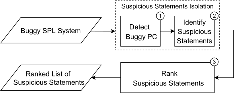
Figure 2: VarCop’s Overview

2.3 VarCop Overview

Based on these observations, we propose VarCop, a novel variability fault localization approach. For a given buggy SPL system, the input of VarCop consists of a set of the tested products and their program spectra. VarCop outputs a ranked list of suspicious statements in three steps (Fig. 2):

1. First, by analyzing the configurations and the overall test results of the sampled products, VarCop detects minimal sets of features whose selections (the states of being on/off) make the bugs (in)visible. Let us call such a set of selections a Buggy Partial Configuration (Buggy PC). In Fig. 1, $\{Weight=T$, $Overloaded=T$, $TwoThirdsFull=F\}$ is a Buggy PC.

2. Next, for each failing product, VarCop aims to isolate the suspicious statements which are responsible for implementing the interaction among the features in each detected Buggy PC. Specially, the feature interaction implementation is a set of the statements which these features use to impact each other. For example, in $p_{7}$, VarCop analyzes its code to detect the implementation of the interaction among Weight, Overloaded, and TwoThirdsFull (O1 and O2), and this interaction implementation includes the statements at lines 9, 15, and 31. Intuitively, all the statements in $p_{7}$ which have an impact on these statements or are impacted by them are also suspicious.

3. Finally, the suspicious statements are ranked by examining how their suspiciousness exposes in both the overall test results of the containing products (product-based suspiciousness assessment) and these products’ detailed case-by-case test results (test case-based suspiciousness assessment). Particularly, for each isolated statement, the product-based assessment is calculated based on the numbers of the passing and failing products containing the statement. Meanwhile, the test case-based suspiciousness is assessed by aggregating the suspiciousness scores of the statement in the failing products which are calculated based on the detailed results of the tests executed by the statement. (O3).

3 Concepts and Problem Statement

A software product line is a product family that consists of a set of products sharing a common code base. These products distinguish from the others in terms of their features [1].

Definition 3.1.

(Software Product Line System). A Software Product Line System (SPL) $\mathfrak{S}$ is a 3-tuple $\mathfrak{S}=\langle\mathbb{S},\mathbb{F},\varphi\rangle$, where:

• $\mathbb{S}$ is a set of code statements that are used to implement $\mathfrak{S}$.

• $\mathbb{F}$ is a set of the features in the system. A feature selection of a feature $f\in\mathbb{F}$ is the state of being either enabled (on) or disabled (off) ($f=T/F$ for short).

• $\varphi:\mathbb{F}\to 2^{\mathbb{S}}$ is the feature implementation function. For a feature $f\in\mathbb{F}$, $\varphi(f)\subset\mathbb{S}$ refers to the implementation of $f$ in $\mathfrak{S}$, and $\varphi(f)$ is included in the products where $f$ is on.

A set of the selections of all the features in $\mathbb{F}$ defines a configuration. Any non-empty subset of a configuration is called a partial configuration. A configuration specifies a single product. For example, configuration $c_{1}=\{Empty=F,Weight=T,TwoThirdsFull=F,Overloaded=F\}$ specifies product $p_{1}$. A product is the composition of the implementation of all the enabled features, e.g., $p_{1}$ is composed of $\varphi(Base)$ and $\varphi(Weight)$.

We denote the sets of all the possible valid configurations and all the corresponding products of $\mathfrak{S}$ by $\mathbb{C}$ and $\mathbb{P}$, respectively ($|\mathbb{C}|=|\mathbb{P}|$). In practice, a subset of $\mathbb{C}$, $C$ (the corresponding products $P\subset\mathbb{P}$), is sampled for testing and finding bugs. Unlike non-configurable code, bugs in SPL systems can be variable and only cause the failures in certain products. In Table I, the bug at line 31 only causes the failures in $p_{6}$ and $p_{7}$. This bug is a variability bug. In the rest of this paper, we simply call an SPL system containing variability bugs a buggy system. In this work, we localize bugs at the statement-level [26], which is the granularity widely adopted in the existing studies [11, 27, 17, 28].

Definition 3.2.

(Variability Bug). Given a buggy SPL system $\mathfrak{S}$ and a set of products of the system, $P$, which is sampled for testing, a variability bug is an incorrect code statement of $\mathfrak{S}$ that causes the unexpected behaviors (failures) in a set of products which is a non-empty strict subset of $P$.

In other words, $\mathfrak{S}$ contains variability bugs if and only if $P$ is categorized into two separate non-empty sets based on their test results: the passing products $P_{P}$ and the failing products $P_{F}$ corresponding to the passing configurations $C_{P}$ and the failing configurations $C_{F}$, respectively. Every product in $P_{P}$ passes all its tests, while each product in $P_{F}$ fails at least one test. Note that $P_{P}\cup P_{F}=P$ and $C_{P}\cup C_{F}=C$. In Table I, $P_{P}=\{p_{1},p_{2},$ $p_{3},p_{4},p_{5}\}$, and $P_{F}=\{p_{6},p_{7}\}$. Besides the test results, the statements of every product executed by each test are also recorded to localize bugs. This execution information is called program spectra [29].

From the above basic concepts, the problem of variability fault localization is defined as follows:

Definition 3.3.

(Variability Bug Localization). Given 3-tuple $\langle\mathfrak{S},P,R\rangle$, where:

• $\mathfrak{S}=\langle\mathbb{S},\mathbb{F},\varphi\rangle$ is a system containing variability bugs.

• $P=\{p_{1},p_{2},...,p_{n}\}$ is the set of sampled products, $P=P_{P}\cup P_{F}$, where $P_{P}$ and $P_{F}$ are the sets of passing and failing products of $\mathfrak{S}$.

• $R=\{R_{1},R_{2},...,R_{n}\}$ is the set of the program spectra of the products in $P$, where $R_{i}$ is the program spectra of $p_{i}$.

Variability Bug Localization is to output the list of the statements in $\mathfrak{S}$ ranked based on their suspiciousness to be buggy.

4 Feature Interaction

We introduce our feature interaction formulation used in this work to analyze the root cause of variability bugs.

4.1 Feature Interaction Formulation

Different kinds of feature interactions have been discussed in the literature [25, 3, 7, 30]. In this work, we formulate feature interaction based on the impacts of a feature on other features. Specially, for a set of features in a product, a feature can interact with the others in two ways: (i) directly impacting the others’ implementation and (ii) indirectly impacting the others’ behaviors via the statements which are impacted by all of them. For (i), there is control/data dependency between the implementation of these features. For example, in $p_{5}$, since the statement at line 26 ($s_{26}$) in $\varphi(TwoThirdsFull)$ is data-dependent on $s_{9}$ and $s_{15}$ in $\varphi(Weight)$, there is an interaction between $Weight$ and $TwoThirdsFull$ in $p_{5}$. For (ii), there is at least one statement which is control/data dependent on a statement(s) of every feature in the set. For instance, in $p_{5}$, $TwoThirdsFull$ and $Weight$ interact by both impacting the statement at line 31. As a result, when these features are all on in a product, each of them will impact the others’ behaviors.

Without loss of generality, a statement can be considered to be impacted by that statement itself. Thus, for a set of enabled features $F$, in a product, there exists an interaction among these features if there is a statement $s$ which is impacted by the implementation of all the features in $F$, regardless of whether $s$ is used to implement these features or not. Formally, we define impact function, $\Omega$, to determine the impact of a statement in a product.

Definition 4.1.

(Impact Function). Given a system $\mathfrak{S}=\langle\mathbb{S},\mathbb{F},\varphi\rangle$, we define impact function as $\Omega:\mathbb{S}\times\mathbb{P}\to 2^{\mathbb{S}}$. Specially, $\Omega(s,p)$ refers to the set of the statements of $\mathfrak{S}$ which are impacted by statement $s$ in product $p$. For a statement $s^{\prime}$ in product $p$, $s^{\prime}\in\Omega(s,p)$ if $s^{\prime}$ satisfies one of the following conditions:

• $s^{\prime}=s$

• $s^{\prime}$ is data/control-dependent on $s$

For our example, $\Omega(s_{33},p_{5})=\{s_{33},s_{36},s_{37},s_{38}\}$. Note that if statement $s$ is not in product $p$, then $\Omega(s,p)=\emptyset$.

Definition 4.2.

(Feature Interaction). Given a system $\mathfrak{S}=\langle\mathbb{S},\mathbb{F},\varphi\rangle$, for product $p$ and a set of features $F$ which are enabled in $p$, the interaction among the features in $F$ exists if and only if the following condition is satisfied:

$$\bigcap_{f\in F}\alpha(f,p)\neq\emptyset$$

where $\alpha(f,p)=\bigcup_{s\in\varphi(f)}\Omega(s,p)$ refers to the set of the statements in $p$ which are impacted by any statement in $\varphi(f)$. The implementation of the interaction among features $F$ in product $p$ is denoted by $\beta(F,p)=\bigcap_{f\in F}\alpha(f,p)$.

For the example in Fig. 1, the features $Weight$ and $Overloaded$ interact with each other in product $p_{7}$ and the implementation of the interaction includes the statements at lines 31–33 and 36–38. Note that, without loss of generality, a feature can impact and interact with itself.

4.2 The Root Cause of Variability Failures

In this section, we analyze and discuss the relation between variability failures in SPL systems and the enabling/disabling of system features. In a buggy SPL system, the variability bugs can be revealed by set(s) of the relevant features which must be enabled and disabled together to make the bugs visible. For each set of relevant features, their selections might affect the visibility of the bugs in the system. For simplicity, we first analyze the buggy system containing a single set of such relevant features. The cases where multiple sets of relevant features involve in the variability failures will be discussed in the later part.

Let consider the cases where the failures of a system are revealed by a single set of the relevant features, $F_{r}=F_{E}\cup F_{D}$, where the features in $F_{E}$ and $F_{D}$ must be respectively enabled and disabled together to make the bugs visible. Specially, the features in $F_{E}$ and $F_{D}$ must be respectively on and off in all the failing products. From a failing product $p\in P_{F}$, once switching the current selection of any switchable feature in $F_{r}$, the resulting product $p^{\prime}$ will pass all its tests, $p^{\prime}\in P_{P}$. In this case, the interaction of features in $F_{r}$ propagates the impact of buggy statements to the actual outputs causing the failures in $p$. The relation between variability bugs (buggy statements) causing the failures in failing products and the interaction between the relevant features in $F_{r}$ will be theoretically discussed as following.

For a failing product $p\in P_{F}$, we denote the set of the buggy statements in $p$ by $\mathcal{S}_{b}$. From $p$, disabling any feature $f_{e}\in F_{E}$ would produce a passing product $p^{\prime}\in P_{P}$. In this case, every buggy statement $s\in\mathcal{S}_{b}$ can be either present or not in $p^{\prime}$. First, if $s$ is not in $p^{\prime}$ after disabling $f_{e}$ from $p$, then $s\in\varphi(f_{e})\subseteq\alpha(f_{e},p)$. The second case is that $s$ is still in $p^{\prime}$. Due to the absence of $f_{e}$, $s$ behaves differently from the way it does incorrectly in $p$, and $p^{\prime}$ passes all its tests. This means, in $p$, $f_{e}$ has impact on $s$ and/or the statements impacted by $s$, $\Omega(s,p)$. In other words, $\alpha(f_{e},p)\cap\Omega(s,p)\neq\emptyset$. In $p$, $s$ and the statements impacted by $s$ together propagate their impacts to the unexpected outputs in $p$. Thus, any change on the statements in $\Omega(s,p)$ can affect the bugs’ visibility.

These two above cases show that every incorrect statement $s$ in $\mathcal{S}_{b}$, only exposes its bugginess with the presence of all the features in $F_{E}$. This demonstrates that the features in $F_{E}$ must interact with each other in $p$, $\beta(F_{E},p)=\bigcap_{f_{e}\in F_{E}}\alpha(f_{e},p)\neq\emptyset$. Indeed, if there exists a feature $f\in F_{E}$ which does not interact with the others in $F_{E}$, $\alpha(f,p)\cap\beta(F_{E}\setminus\{f\},p)=\emptyset$, the incorrect behaviors of $s$ will only be impacted by either $f$ or the interaction among the features in {$F_{E}\setminus{f}\}$. As a result, $s$ will not require the presence of both $f$ and $\{F_{E}\setminus{f}\}$ to reveal its bugginess. Moreover, since every $f_{e}\in F_{E}$ has impacts on the behaviors of all the buggy statements, $\forall s\in\mathcal{S}_{b}$, $\forall f_{e}\in F_{E},\Omega(s,p)\cap\alpha(f_{e},p)\neq\emptyset$, the interaction among the features in $F_{E}$ also has impacts on the behaviors of every buggy statement, $\forall s\in\mathcal{S}_{b}$, $\Omega(s,p)\cap\beta(F_{E},p)\neq\emptyset$. In other words, the features $F_{E}$ interact with each other in $p$, and the interaction implementation impacts the visibility of the failures caused by every buggy statement. Hence, the statements which implement the interaction among the features in $F_{E}$ are valuable suggestions to localize the buggy statements. This theoretically confirms our observation O1.

Similarly, from $p$, turning on any disabled feature $f_{d}\in F_{D}$, the resulting product $p^{\prime\prime}$ also passes all its tests. This illustrates that in $p^{\prime\prime}$, the behaviors of every buggy statement $s$ in $\mathcal{S}_{b}$ are impacted by the presence of $f_{d}$, thus the incorrect behaviors of $s$ cannot be exposed. Formally, $\forall s\in\mathcal{S}_{b},\Omega(s,p)\cap\alpha(f_{d},p^{\prime\prime})\neq\emptyset$. Intuitively, $f_{d}$ has impacts on interaction implementation of $F_{E}$ in $p$ as well as the impact of this interaction on $\Omega(s,p)$. In other words, the interaction among $F_{E}\cup F_{D}$ impacts the behaviors of the buggy statements, $\forall s\in\mathcal{S}_{b}$, $\Omega(s,p)\cap\beta(F_{E}\cup F_{D},p^{\prime\prime})\neq\emptyset$. Hence, investigating the interaction implementation of the features in $F_{D}$ and $F_{E}$ (if they were all enabled in a product) can provide us useful indications to find the incorrect statements. This explains our observation O2.

Overall, the interaction among the relevant features in $F_{r}=F_{E}\cup F_{D}$ reveals/hides the bugs by impacting the buggy statements and/or the statements impacted by the buggy ones in the products. Illustratively, this interaction implementation propagates the impact of all the buggy statements to the output of the failed tests in a failing product. This means that the buggy statements are contained in the set of statements which are impacted by or have impacts on the interaction implementation of the relevant features. Thus, identifying the sets of the relevant features whose interaction can affect the variability bugs visible/invisible and the implementation of the interaction is necessary to localize variability bugs in SPL systems.

In general, variability bugs in a system can be revealed by multiple sets of relevant features. In these cases, the visibility of the bugs might not be clearly observed by switching the selections of features in one set of relevant features. For instance, $F_{r}$ and $F_{r}^{\prime}$ are two sets of relevant features whose interaction causes the failures in the system. Once switching the selection of any feature in $F_{r}$, the implementation of the interaction among the features in $F_{r}$ is not in the resulting product $p^{\prime}$. Meanwhile, $p^{\prime}$ can still contain the interaction among the features in $F_{r}^{\prime}$. Thus, $p^{\prime}$ can still fail some tests. However, if we can identify $F_{r}$ and/or $F_{r}^{\prime}$ or even their subsets, by examining the interaction among the identified set(s) of features, the bugs can be isolated. More details will be described and proved in the next section.

In spite of the importance of the relation between variability failures and relevant features, this information is not utilized by existing studies such as SBFL and S-SBFL. Consequently, their resulting suspicious spaces are often large. Meanwhile, by Arrieta et al. [10], SBFL is adapted to localize bugs at the feature-level. Particularly, each sampled product is considered as a test (i.e., passed tests are passing products, and failed tests are failing products), and the spectra record the feature selections in each product. However, SBFL is used to localize the buggy features. By this method, all the statements in the same feature have the same suspiciousness level. Thus, this approach could be ineffective for localizing variability bugs at the statement-level. This will be empirically illustrated in our results (Section 9).

5 Buggy Partial Configuration Detection

In this section, we introduce the notions of Buggy Partial Configuration (Buggy PC) and Suspicious Partial Configuration (Suspicious PC). Specially, Buggy PCs are the partial configurations whose interactions among the corresponding features are the root causes making variability bugs visible in a buggy system. In general, Buggy PCs can be detected after testing all the possible products of the system. However, verifying all those products is nearly impossible in practice. Meanwhile, Suspicious PCs are the detected suspicious candidates for the Buggy PCs which can be practically computed using the sampled products.

5.1 Buggy Partial Configuration

For a buggy system $\mathfrak{S}=\langle\mathbb{S},\mathbb{F},\varphi\rangle$, where all the possible configurations of $\mathfrak{S}$, $\mathbb{C}$, is categorized into the non-empty sets of passing ($\mathbb{C}_{P}$) and failing ($\mathbb{C}_{F}$) configurations, $\mathbb{C}_{P}\cup\mathbb{C}_{F}=\mathbb{C}$, a Buggy Partial Configuration (Buggy PC) is the minimal set of feature selections that makes the bugs visible in the products. In Fig. 1, the only Buggy PC is $B=\{Weight=T,TwoThirdsFull=F,Overloaded=T\}$.

Definition 5.1.

(Buggy Partial Configuration (Buggy PC)). Given a buggy system $\mathfrak{S}=\langle\mathbb{S},\mathbb{F},\varphi\rangle$, a buggy partial configuration, $B$, is a set of feature selections in $\mathfrak{S}$ that has both the following Bug-Revelation and Minimality properties:

• Bug-Revelation. Any configuration containing $B$ is corresponding to a failing product, $\forall c\in\mathbb{C},c\supseteq B\implies c\in\mathbb{C}_{F}$.

• Minimality. There are no strict subsets of $B$ satisfying the Bug-Revelation property, $\forall B^{\prime}\subsetneq B\implies\neg(\forall c\in\mathbb{C},c\supseteq B^{\prime}\implies c\in\mathbb{C}_{F})$.

Bug-Revelation. This property is equivalent to that all the passing configurations do not contain $B$. Indeed,

$$\forall c\in\mathbb{C},c\supseteq B\implies c\in\mathbb{C}_{F}$$

$$\Leftrightarrow\forall c\in\mathbb{C},[c\not\supseteq B\vee c\in\mathbb{C}_{F}]$$

$$\Leftrightarrow\forall c\in\mathbb{C},[c\not\supseteq B\vee c\not\in\mathbb{C}_{P}]$$

$$\Leftrightarrow\forall c\in\mathbb{C},c\in\mathbb{C}_{P}\implies c\not\supseteq B$$

For a set of feature selections $B^{\prime}$, if there exists a passing configuration containing $B^{\prime}$, $\exists c\in\mathbb{C}_{P}\wedge c\supset B^{\prime}$, the interaction among the features in $B^{\prime}$ in the corresponding product $p$ cannot be the root cause of any variability bug. This is because there is no unexpected behavior caused by this interaction in the passing product $p$. Hence, investigating the interaction between them might not help us localize the bugs. For example, $B^{\prime}=$ $\{Empty=T,Weight=T\}$ is a subset of the failing configuration $c_{6}$, however it is not considered as a Buggy PC, because $B^{\prime}$ also is a subset of $c_{2}$ which is a passing configuration. Indeed, in every product, the interaction between $Empty$ and $Weight$, which does not cause any failure, should not be investigated to find the bug. Thus, to guarantee that the interaction among the features in a Buggy PC is the root cause of variability bugs, the set of feature selections needs to have Bug-Revelation property.

Minimality. If a set $B$ holds the Bug-Revelation property but not minimal, then there exists a strict subset $B^{\prime}$ of $B$ ($B^{\prime}\subsetneq B$) that also has Bug-Revelation property. However, for any $p\in P_{F}$ whose configuration contains both $B$ and $B^{\prime}$, to detect all the bugs related to either $B$ or $B^{\prime}$, the smaller one, $B^{\prime}$, should still be examined rather than $B$. The reason is, in $p$, the bugs related to both $B$ and $B^{\prime}$ are all covered by the implementation of the interaction among the features in $B^{\prime}$.

Particularly, let $B^{\prime}=F^{\prime}_{E}\cup F^{\prime}_{D}$ and $B=F_{E}\cup F_{D}$, where $F^{\prime}_{E}$, $F^{\prime}_{D}$, $F_{E}$, and $F_{D}$ are the sets of enabled and disabled features in $B^{\prime}$ and $B$, respectively. Since $B^{\prime}\subset B$, and $F^{\prime}_{E}\cap F^{\prime}_{D}=F_{E}\cap F_{D}=\emptyset$, we have $F^{\prime}_{E}\subseteq F_{E}$ and $F^{\prime}_{D}\subseteq F_{D}$. For the enabled features in $F_{E}$ and $F^{\prime}_{E}$, the failures in $p$ can be caused by the interactions among the enabled features in $F_{E}$ or $F^{\prime}_{E}$. The implementation of the interactions among the enabled features in $F_{E}$ and $F^{\prime}_{E}$ in $p$ are $\beta(F_{E},p)=\bigcap_{f\in F_{E}}\alpha(f,p)$ and $\beta(F^{\prime}_{E},p)=\bigcap_{f^{\prime}\in F^{\prime}_{E}}\alpha(f^{\prime},p)$, respectively. Then, we have $\beta(F_{E},p)\subseteq\beta(F^{\prime}_{E},p)$ because $F^{\prime}_{E}\subseteq F_{E}$. As a result, the incorrect statements related to $\beta(F_{E},p)$ are all included in $\beta(F^{\prime}_{E},p)$. Similarly, for the sets of the disabled features, the set of the statements in $p$ related to all the features of $F^{\prime}_{D}$ also includes the statements related to all the features of $F_{D}$. In consequence, by identifying the interaction implementation of the features in $B^{\prime}$, the bugs which are related to both $B$ and $B^{\prime}$ can all be found.

Furthermore, if both $B$ and $B^{\prime}$ are related to the same bug(s), the larger set could contain bug-irrelevant feature selections which can negatively affect the FL effectiveness. For example, both the entire configuration $c_{6}$ and its subset $\{TwoThirdsFull=F,Overloaded=T,Weight=T\}$ has Bug-Revelation property. Nevertheless, the interaction among $TwoThirdsFull$, $Overloaded$, and $Weight$, which indeed causes the failures in $p_{6}$, should be investigated instead of the interaction among the features in the entire $c_{6}$. This configuration contains the bug-irrelevant selection, $Empty=T$. As a result, Buggy PCs need to be minimal.

Buggy PC Detection Requirement. All possible configurations of a system are very rarely available for the QA process. Thus, in a buggy system, the sampled set is used to detect the Buggy PCs. Assuming that $\mathbb{D}$ is the set of the candidates for Buggy PCs which is detected by an FL approach. For any $D\in\mathbb{D}$, all the statements which implement the interaction among the features in $D$ and the statements which have impact on that interaction implementation (Section 4.2) are suspicious. Thus, for a Buggy PC $B$, to avoid missing related buggy statements $\mathcal{S}$, the FL method must ensure that $\mathcal{S}$ is covered by the suspicious statements identified from least one candidate: there must be at least one candidate in $\mathbb{D}$ which is a subset of $B$, $\exists D\in\mathbb{D}$, $D\subseteq B$. Let us call this the effectiveness requirement.

Indeed, if there exists $D\in\mathbb{D}$, such that $D\subseteq B$, then in a product $p$ whose configuration contains $B$ (apparently contains $D$), the interaction implementation of the features in $D$ covers all the statements implementing the interaction of the features in $B$, $\beta(D,p)\supseteq\beta(B,p)$. As a result, the suspicious statements set of $D$ contains both the interaction implementation $\beta(B,p)$ and the statements which have impact on this interaction in $p$. In other words, the suspicious statements set of $D$ contains buggy statements $\mathcal{S}$. Hence, to guarantee the effectiveness in localizing variability bugs, we aim to detect the set of the candidates for Buggy PCs which satisfies the effectiveness requirement.

5.2 Important Properties to Detect Buggy PC

In practice, a system $\mathfrak{S}$ may have a huge number of possible configurations, $\mathbb{C}$. Consequently, only a subset of $\mathbb{C}$ is sampled for testing and debugging, $C=C_{P}\cup C_{F}$. A set of feature selections which has both Bug-Revelation and Minimality properties on the sampled set $C$ is intuitively suspicious to be a Buggy PC. Let us call these sets of selections Suspicious Partial Configurations (Suspicious PCs).

For example, in Fig. 1, $D=\{TwoThirdsFull=F,Overloaded=T\}$ is a Suspicious PC. All the configurations containing $D$ ($c_{6}$ and $c_{7}$) are failing. Additionally, all the strict subsets of $D$ do not hold Bug-Revelation on $C$, e.g., $\{TwoThirdsFull=F\}$ is in $c_{1}$, and $\{Overloaded=T\}$ is in $c_{5}$, which are passing configurations. Thus, $D$ is a minimal set which holds the Bug-Revelation property on $C$.

Theoretically, the Suspicious PCs in $c$ can be detected by examining all of its subsets to identify the sets satisfying both Bug-Revelation and Minimality. The number of sets that need to be examined could be $2^{|c|}-1$. However, not every selection in $c$ participates in Suspicious PCs. Hence, to detect Suspicious PCs efficiently, we aim to identify a set of the selections, $SFS_{c}$, (Suspicious Feature Selections) of $c$ in which the selections potentially participate in one or more Suspicious PCs. Then, instead of inefficiently examining all the possible subsets of $c$, the subsets of $SFS_{c}$, which is a subset of $c$, are inspected to identify Suspicious PCs.

Particularly, in failing configuration $c$, there exist the selections such that switching their current states (from on to off, or vice versa) results in a passing configuration $c^{\prime}$. In other words, the bugs in the product of $c$ are invisible in the product corresponding to $c^{\prime}$, and the resulting product passes all its tests. Intuitively, each of these selections might be relevant to the visibility of the bugs. Each of these selections can be considered as a Suspicious Feature Selection. Thus, a selection, which is in a failing configuration yet not in a passing one, is suspicious to the visibility of the bugs.

Definition 5.2.

(Suspicious Feature Selection (SFS)). For a failing configuration $c\in C_{F}$, a feature selection $f_{s}\in c$ is suspicious if $f_{s}$ is not present in at least one passing configuration, formally $\exists c^{\prime}\in C_{P},f_{s}\not\in c^{\prime}$, specially, $f_{s}\in c\setminus c^{\prime}$.

For example, the $SFS_{7}$ of $c_{7}$ contains the selections in the set differences of $c_{7}$ and the passing configurations, e.g., $c_{7}\setminus c_{1}=\{Overloaded=T\}$. Intuitively, the set difference $(c_{7}\setminus c_{1})$ must contain a part of every Buggy PC in $c_{7}$, otherwise $c_{1}$ would contain a Buggy PC and fail some tests. Hence, for any failing configuration $c$, we have the following property about the relation between the set of the Buggy PCs in $c$ and $(c\setminus c^{\prime})$ where $c^{\prime}$ is a passing configuration.

Property 5.1.

Given failing configuration $c$ whose set of the Buggy PCs is $BPC_{c}$, the difference of $c$ from any passing configuration $c^{\prime}$ contains a part of every Buggy PC in $BPC_{c}$. Formally, $\forall c^{\prime}\in C_{P},\forall B\in BPC_{c},(c\setminus c^{\prime})\cap B\neq\emptyset$.

The intuition is that for a failing configuration $c$ and a passing one $c^{\prime}$, a Buggy PC in $c$ can be either in their common part ($c\cap c^{\prime}$) or their difference part ($c\setminus c^{\prime}$). As $c^{\prime}$ is a passing configuration, the difference must contain a part of every Buggy PC in $c$. Otherwise, there would exist a Buggy PC in both $c$ and $c^{\prime}$, and $c^{\prime}$ should be a failing configuration (Bug-Revelation property). This is impossible.

For a configuration $c\in C_{F}$, we denote $SFS_{c}$ as the set of all the suspicious feature selections of $c$, $SFS_{c}=\bigcup_{c^{\prime}\in C_{P}}(c\setminus c^{\prime})$. To detect Buggy PCs in $c$, we identify all subsets of $SFS_{c}$ which satisfy the Bug-Revelation and Minimality properties regarding to $C$. The following property demonstrates that our method maintains the effectiveness requirement in detecting Buggy PCs (Section 5.1).

Property 5.2.

Given a failing configuration $c$ whose set of the Buggy PCs is $BPC_{c}$, for any $B\in BPC_{c}$, there exists a subset of $SFS_{c}$, $M\subseteq SFS_{c}$, such that $M$ satisfies the Bug-Revelation condition in the sampled set $C$ and $M\subseteq B$.

Proof.

Considering a Buggy PC of a failing configuration $c$, $B\in BPC_{c}$, we denote $(c\setminus c^{\prime})\cap B$ by $M_{c^{\prime}}\neq\emptyset$, where $c^{\prime}$ is a passing configuration (Property 5.1). Let consider $M=\bigcup_{c^{\prime}\in C_{P}}M_{c^{\prime}}$. Note that, as $M_{c^{\prime}}\subseteq(c\setminus c^{\prime})$, we have $M\subseteq SFS_{c}=\bigcup_{c^{\prime}\in C_{P}}(c\setminus c^{\prime})$. In addition, since $M_{c^{\prime}}\subset B$ for every passing configuration $c^{\prime}\in C_{P}$, we have $M\subset B$. Moreover, for every passing configuration $c^{\prime}\in C_{P}$, because $c^{\prime}\not\supset M_{c^{\prime}}$ (since $M_{c^{\prime}}\subset(c\setminus c^{\prime})$), $c^{\prime}$ does not contain any superset of $M_{c}$, then $c^{\prime}\not\supset M$. As a result, $M$, which is a subset of both $SFS_{c}$ and $B$, satisfies Bug-Revelation property.

∎

As a result, given $c\in C_{F}$, there always exists a common subset of $SFS_{c}$ and $B$, for any $B\in BPC_{c}$, and that set satisfies Bug-Revelation property on $C$. Hence, according to the effectiveness requirement (Section 5.1), detecting Buggy PCs by examining the subsets of $SFS_{c}$ is effective to localize the variability bugs. Furthermore, as $SFS_{c}$ only contains the differences of $c$ and other passing configurations, $|SFS_{c}|\leq|c|$. For example in Table I, SFSs of configuration $c_{6}$ is $SFS_{6}=\{Empty=T,Weight=T,TwoThirdsFull=F,Overloaded=T\}$, so $|SFS_{6}|<|c_{6}|$. Thus, $SFS_{c}$ should be used to detect Buggy PCs rather than $c$.

Note that Suspicious PCs and Buggy PCs all hold the Bug-Revelation on the given sampled set of configurations, $C$. However, because there are some (passing) configurations in $\mathbb{C}$ but not in $C$, it does not express that some selections must be in a Buggy PC. Hence, Buggy PCs might not hold Minimality property on $C$. In Fig. 1, a Buggy PC is $B=\{Weight=T,TwoThirdsFull=F,Overloaded=T\}$. However, $B$ does not satisfy Minimality on the set of the available configurations (Table I), because its subset, $\{TwoThirdsFull=F,Overloaded=T\}$, satisfies Bug-Revelation on $C$. The reason is that Table I does not show any product whose configuration contains both $\{Weight=F\}$ as well as $\{TwoThirdsFull=F,Overloaded=T\}$ passes or fails their tests. Therefore, $\{Weight=T\}$ is not expressed as a part of the Buggy PC.

5.3 Buggy PC Detection Algorithm

Algorithm 1 describes our algorithm to detect Buggy PCs and return the Suspicious PCs in a buggy system, given the sets of the passing and failing configurations, $C_{P}$ and $C_{F}$.

1

2 Procedure DetectBuggyPCs($C_{P}$, $C_{F}$)

3       $SuspiciousPCSets=\emptyset$

4       for $c\in C_{F}$ do

5             $SFS_{c}=\emptyset$

6             for $c^{\prime}\in C_{P}$ do

7                   $F_{S}=c\setminus c^{\prime}$

8                   $SFS_{c}=SFS_{c}\cup F_{S}$

9                  

10             end for

11            for $k\in[1,K]$ do

12                   $S_{k}=subsetWithSize(SFS_{c},k)$

13                   for ($cand\in S_{k})\wedge(\nexists spc\in SuspiciousPCSets,cand\supset spc)$ do

14                         if  $satisfy(cand,C_{P},C_{F})$ then

15                               $SuspiciousPCSets.add(cand)$

16                              

17                         end if

18                        

19                   end for

20                  

21             end for

22            

23       end for

24      

25      return $SuspiciousPCSets$

26

27

Algorithm 1 Buggy PC Detection Algorithm

In Algorithm 1, all the Suspicious PCs in the system are collected from the Suspicious PCs identified in each failing configuration $c$ (lines 3–17). From lines 4–8, the set of the suspicious selections in $c$ is computed. In order to do that, the differences of $c$ from all the passing configurations are gathered and stored in $SFS_{c}$ (lines 5–8).

Next, the Suspicious PCs in $c$ are the subsets of $SFS_{c}$ which have both Bug-Revelation and Minimality with respect to $C=C_{F}\cup C_{P}$ (lines 12–14). Each candidate, a set of feature selections $cand$, is checked against these properties by $satisfy$ (line 12). In Algorithm 1, the examined subsets of $SFS_{c}$ have the maximum size of $K$ (lines 9–10). In other words, the considered interactions are up to $K$-way. In practice, most of the bugs are caused by the interactions of fewer than 6 features [3, 31]. Thus, one should set $K=\textit{7}$ to ensure the efficiency. Specially, the function $subsetWithSize(SFS_{c},k)$ (line 10) returns all the subsets size $k$ of $SFS_{c}$. Note that if a set is already a Suspicious PC, then any superset of it would not be a Suspicious PC (violating Minimality). Thus, all the supersets of the identified Suspicious PCs can be early eliminated (line 11).

In our example, from Table I, the detected Suspicious PCs are two sets $D_{1}=\{\textit{TwoThirdsFull}=F,\textit{Overloaded}=T\}$ and $D_{2}=\{\textit{Empty}=T,\textit{Overloaded}=T\}$.

6 Suspicious Statements Identification

For a buggy SPL system, the incorrect statements can be found by examining the statements which implement interactions of Buggy PCs as well as the statements impacting that implementation, as discussed in Section 4.2. Thus, all the statements which implement the interactions of Suspicious PCs and the statements impacting them, are considered as suspicious to be buggy. In a product $p\in P_{F}$, for a Suspicious PC $D$ whose the sets of enabled and disabled features are $F_{E}$ and $F_{D}$, respectively. Hence, in $p$, the interaction implementation of $D$ includes the statements implementing the interaction of $F_{E}$ which can be impacted by the features in $F_{D}$ (if the disabled features were on in $p$).

In practice, the features in $F_{D}$ can be mutually exclusive with other features enabled in $p$, which is constrained by the feature model [1]. Thus, the impact of $F_{D}$ on the implementation of the interaction of $F_{E}$ in $p$, $\beta(F_{E},p)$ might not be easily identified via the control/data dependency in $p$. In this work, the impacts of the features in $F_{D}$ on statements in $p$ are approximately identified by using def-use relationships of the variables and methods that are shared between the features in $F_{D}$ and $p$ [7]. Formally, for a statement $s$, we denote $def(s)$ and $use(s)$ to refer to the sets of variables/methods defined and used by $s$, respectively.

Definition 6.1.

(Def-Use Impact). Given an SPL system $\mathfrak{S}=\langle\mathbb{S},\mathbb{F},\varphi\rangle$ and its sets of products $\mathbb{P}$, we define the def-use impact function as $\gamma$: $\mathbb{F}\times\mathbb{P}\to 2^{\mathbb{S}}$, where $\gamma(f,p)$ refers to the set of the statements in $p$ which are impacted by any statement in the implementation of feature $f$, $\varphi(f)$, via the variables/methods shared between $\varphi(f)$ and $p$. Formally, for a statement $s$ in product $p$, $s\in\gamma(f,p)$ if one of the following conditions is satisfied:

• $\exists t\in\varphi(f)$, $def(t)\cap use(s)\neq\emptyset$

• s is data/control-dependent on s’, and $s^{\prime}\in\gamma(f,p)$

In summary, in a product $p\in P_{F}$, for a Suspicious PC whose the sets of enabled and disabled features are $F_{E}$ and $F_{D}$, the suspicious statements satisfy the following conditions: (i) implementing the interaction of the features in $F_{E}$ and $F_{D}$ or impacting this implementation; (ii) executing the failed tests of $p$. For a buggy system, the suspicious space contains all the suspicious statements detected for all Suspicious PCs in every failing product.

7 Suspicious Statements Ranking

To rank the isolated suspicious statements of a buggy system, VarCop assigns a score to each of these statements based on the program spectra of the sampled products. In VarCop, the suspiciousness of each statement is assessed based on two criteria/dimensions: Product-based Assessment and Test Case-based Assessment.

7.1 Product-based Suspiciousness Assessment

This criterion is based on the overall test results of the products containing the statement. Specially, in a buggy system, a suspicious statement $s$ could be executed in not only the failing products but also the passing products. Hence, from the product-based perspective, the (dis)appearances of $s$ in the failing and passing products could be taken into account to assess the statement’s suspiciousness in the whole system. In general, the product-based suspiciousness assessment for $s$ could be derived based on the numbers of the passing and failing products where $s$ is contained or not. Intuitively, the more failing products and the fewer passing products where $s$ is contained, the more suspicious $s$ tend to be. This is similar to the idea of SBFL when considering each product as a test. Thus, in this work, we adopt SBFL metrics to determine the product-based suspiciousness assessment for $s$. Specially, for a particular SBFL metric $M$, the value of this assessment is determined by $ps(s,M)$ which adopts the formula of $M$ with the numbers of the passing and failing products containing and not containing $s$ as the numbers of passed and failed tests executed or not executed by $s$.

7.2 Test Case-based Suspiciousness Assessment

The test case-based suspiciousness of a statement $s$ is evaluated based on the detailed results of the tests executed by $s$. Particularly, in each failing product containing $s$, the statement is locally assessed based on the program spectra of the product. Then, the local scores of $s$ in the failing products are aggregated to form a single value which reflects the test case-based suspiciousness of $s$ in the whole system.

Particularly, the local test case-based suspiciousness of statement $s$ can be calculated by using the existing FL techniques such as SBFL [11, 14, 15, 16, 17]. In this work, we use a ranking metric of SBFL, which is the state-of-the-art FL technique, to measure the local test case-based suspiciousness of $s$ in a failing product. Next, for a metric $M$, the aggregated test case-based suspiciousness of $s$, $ts(s,M)$, can be calculated based on the local scores of $s$ in all the failing products containing it. In general, we can use any aggregation formula [32], such as arithmetic mean, geometric mean, maximum, minimum, and median to aggregate the local scores of $s$.

However, the local test case-based scores of a statement, which are measured in different products, should not be directly aggregated. The reason is that the scores of the statement in different products might be incomparable. Indeed, with some ranking metrics such as Op2 [33] or Dstar [34], once the numbers of tests of the products are different, the local scores of the statements in these products might be in significantly different ranges. Intuitively, if these local scores are directly aggregated, the products which have larger ranges will have more influence on the suspiciousness score of the statement in the whole system. Meanwhile, such larger-score-range products are not necessarily more important in measuring the overall test case-based suspiciousness of the statement. Directly aggregating these incomparable local scores of the statement can result in an inaccurate suspiciousness assessment. Thus, to avoid this problem, these local scores in each product should be normalized into a common scale, e.g., $[0,1]$, before being aggregated. We will show the impact of the normalization as well as choosing the aggregation function and ranking metric on VarCop’s performance in Section 9.2.

7.3 Assessment Combination

Finally, the two assessment scores $ps(s,M)$ and $ts(s,M)$ of statement $s$ are combined with a combination weight, $w\in[0,1]$ to form a single suspiciousness score of the statement:

$$score(s,M)=w*ps(s,M)+(1-w)*ts(s,M)$$

Note that, to avoid the bias caused by the range-difference between the two criteria, these two scores should be normalized into a common range, e.g., $[0,1]$ before the interpolation. In the ranking process, the isolated suspicious statements are ranked according to their interpolated suspiciousness score $score(s,M)$. The impact of the combination weight $w$ on VarCop’s fault localization performance will be empirically shown in Section 9.2.

8 Empirical Methodology

To evaluate our variability fault localization approach, we seek to answer the following research questions:

RQ1: Accuracy and Comparison. How accurate is VarCop in localizing variability bugs? And how is it compared to the state-of-the-art approaches [10, 14, 9]?

RQ2: Intrinsic Analysis. How do the components including the suspicious statement isolation, the normalization, the suspiciousness aggregation function, and the combination weight contribute to VarCop’s performance?

RQ3: Sensitivity Analysis. How do various factors affect VarCop’s performance including the size of sampled product set and the size of test suite in each sampled product?

RQ4: Performance in Localizing Multiple Bugs. How does VarCop perform on localizing multiple variability bugs?

RQ5: Time Complexity. What is VarCop’s running time?

8.1 Dataset

To evaluate VarCop, we conducted several experiments on a large public dataset of variability bugs [18]. This dataset includes 1,570 buggy versions with their corresponding tests of six Java SPL systems which are widely used in SPL studies. There are 338 cases of a single-bug, and 1,232 cases of multiple-bug. The details are shown in Table II.

In the benchmark [18], to generate a large number of variability bugs, the bug generation process includes three main steps: Product Sampling and Test Generating, Bug Seeding, and Variability Bug Verifying. First, for an SPL system, a set of products is systematically sampled by the existing techniques [6]. To inject a fault into the system, a random modification is applied to the system’s original source code by using a mutation operator. Finally, each generated bug is verified against the condition in Definition 3.2 to ensure that the fault is a variability bug and caught by the tests. The detailed design decisions can be found in [18].

To the best of our knowledge, this is the only public dataset containing the versions of the SPL systems that failed by variability bugs found through testing [18]. Indeed, Arrieta et al. [10] also constructed a set of artificial bugs to evaluate their approach in localizing bugs in SPL systems. However, this dataset has not been public. Besides, Abal et al. [23] and Mordahl et al. [24] also published their datasets of real-world variability bugs. However, these datasets are not fit our evaluation well because all of these bugs are not provided along with corresponding test suites, and in fact, most of these bugs are compile-time bugs. Specially, these variability bugs are collected by (manually) investigating bug reports [23] or applying static analysis tools [24].

Before running VarCop on the dataset proposed by Ngo et al. [18], we performed a simple inspection for each case on whether the failures of the system are possibly caused by non-variability bugs. Naturally, there are bugs which may be classified as “variability" because of the low-quality test suites which cannot reveal the bugs in some buggy products. We found that there are 53/1,570 cases (19 single-bug cases and 34 multiple-bug cases) where among the sampled products in each case, the product containing only the base feature and disabling all of the optional features fails several tests. These cases possibly contain non-variability bugs. We will discuss them in Section 9.2.

TABLE II: Dataset Statistics

System	Details		Test info		Bug info
	#LOC	#F	#P	Cov	#SB	#MB
ZipMe	3460	13	25	42.9	55	249
GPL	1944	27	99	99.4	105	267
Elevator-FH-JML	854	6	18	92.9	20	102
ExamDB	513	8	8	99.5	49	214
Email-FH-JML	439	9	27	97.7	36	90
BankAccountTP	143	8	34	99.9	73	310

• #F and #P: Numbers of features and sampled products.

• Cov: Statement coverage (%).

• #SB and #MB: Numbers of single-bug and multiple-bug cases.

8.2 Evaluation Setup, Procedure, and Metrics

8.2.1 Empirical Procedure

Comparative Study. For each buggy version, we compare the performance in ranking buggy statements of VarCop, Arrieta et al. [10], SBFL [11, 14, 15, 16, 17], and the combination of slicing method and SBFL (S-SBFL) [21, 22] accordingly. For SBFL, each SPL system is considered as a non-configurable code. SBFL ranks all the statements executed by failed tests. For S-SBFL, to improve SBFL, S-SBFL isolates all the executed failure-related statements in every failing product by slicing techniques [12] before ranking. A failure-related statement is a statement included in at least a program slice which is backward sliced from a failure point in a failing product. In this experiment, we used 30 most popular SBFL metrics [14, 15, 11]. For each metric, $M$, we compared the performance of all 4 techniques using $M$.

Intrinsic Analysis. We studied the impacts of the following components: Suspicious Statement Isolation, Ranking Metric, Normalization, Aggregation Function, and Combination Weight. We created different variants of VarCop with different combinations and measured their performance.

Sensitivity Analysis. We studied the impacts of the following factors on the performance of VarCop: Sample size and Test set size. To systematically vary these factors, the sample size is varied based on $k$-wise coverage [35] and the numbers of tests are gradually added.

8.2.2 Metrics

We adopted Rank, EXAM [36], and Hit@X [37] which are widely used in evaluating FL techniques [14, 11, 10]. We additionally applied Proportion of Bugs Localized (PBL) [14] for the cases of multiple variability bugs.

Rank. The lower rank of buggy statements, the more effective approach. If there are multiple statements having the same score, buggy statements are ranked last among them. Moreover, for the cases of multiple bugs, we measured Ranks of the first buggy statement (best rank) in the lists.

EXAM. EXAM [36] is the proportion of the statements being examined until the first faulty statement is reached:

$$EXAM=\frac{r}{N}\times 100\%$$

where $r$ is the position of the buggy statement in the ranked list and $N$ is the total number of statements in the list. The lower EXAM, the better FL technique.

Hit@X. Hit@X [37] counts the number of bugs which can be found after investing X ranked statements, e.g., Hit@1 counts the number of buggy statements correctly ranked $1^{st}$ among the experimental cases. In practice, developers only investigate a small number of ranked statements before giving up[38]. Thus, we focus on $X\in[1,5]$.

Proportion of Bugs Localized (PBL). PBL [14] is the proportion of the bugs detected after examining a certain number of the statements. The higher PBL, the better approach.

9 Empirical Results

9.1 Performance Comparison (RQ1)

Table III shows the average performance of VarCop, SBFL, the combination of slicing method and SBFL (S-SBFL), and the feature-based approach proposed by Arrieta et al. [10] (FB) on 338 buggy versions containing a single bug each [18] in Rank and EXAM. The detailed ranking results of each case can be found on our website [39].

TABLE III: Performance of VarCop, SBFL, the combination of Slicing and SBFL (S-SBFL), and Arrieta et al. [10] (FB)

#	Ranking Metric	Rank				EXAM
		VarCop	S-SBFL	SBFL	FB	VarCop	S-SBFL	SBFL	FB
[HTML]C0C0C0 1	Barinel	7.83	9.88	11.48	136.27	2.11	2.87	3.15	21.79
[HTML]C0C0C0 2	Dstar	6.16	7.20	8.09	108.78	1.77	1.94	2.02	15.88
[HTML]C0C0C0 3	Ochiai	6.19	7.25	8.14	109.91	1.77	1.95	2.03	16.10
[HTML]C0C0C0 4	Op2	5.86	6.07	6.74	106.99	1.71	1.75	1.80	15.36
[HTML]C0C0C0 5	Tarantula	6.96	9.88	11.48	136.27	1.98	2.87	3.15	21.79
6	Kulczynski2	5.61	6.36	7.08	108.23	1.67	1.77	1.83	15.59
7	M2	5.94	6.13	6.82	108.43	1.71	1.76	1.81	15.77
8	Harmonic Mean	5.95	6.52	7.28	149.70	1.72	1.80	1.86	21.37
9	Zoltar	6.00	6.12	6.78	107.57	1.68	1.75	1.80	15.45
10	Geometric Mean	6.05	7.37	8.29	149.70	1.76	1.99	2.09	21.37
11	Ample2	6.15	6.16	6.86	149.58	1.75	1.77	1.82	21.30
12	Rogot2	6.22	6.52	7.28	133.66	1.80	1.80	1.86	22.24
13	Sorensen Dice	6.50	8.79	10.17	115.72	1.84	2.41	2.62	17.29
14	Goodman	6.50	8.79	10.17	115.72	1.84	2.41	2.62	17.29
15	Jaccard	6.63	8.79	10.17	115.72	1.83	2.41	2.62	17.29
16	Dice	6.63	8.79	10.17	115.72	1.83	2.41	2.62	17.29
17	Anderberg	6.68	8.79	10.17	115.72	1.84	2.41	2.62	17.29
18	Cohen	6.81	8.93	10.33	152.04	1.87	2.47	2.70	21.61
19	Fleiss	6.82	12.24	52.03	145.70	2.09	3.51	9.13	21.65
20	Simple Matching	6.88	28.00	242.70	158.19	2.11	6.67	30.68	21.96
21	Humman	6.88	28.00	242.70	158.19	2.11	6.67	30.68	21.96
22	Wong2	6.88	28.00	242.70	158.19	2.11	6.67	30.68	21.96
23	Hamming	6.88	28.00	242.70	158.19	2.11	6.67	30.68	21.96
24	Sokal	6.91	28.00	242.70	158.19	2.15	6.67	30.68	21.96
25	Euclid	6.96	28.00	242.70	158.19	2.17	6.67	30.68	21.96
26	Rogers Tanimoto	7.05	28.00	242.70	158.19	2.20	6.67	30.68	21.96
27	Scott	7.38	13.22	50.86	147.65	2.17	3.76	8.79	22.23
28	Rogot1	7.38	13.22	50.86	147.65	2.17	3.76	8.79	22.23
29	Russell Rao	14.06	17.87	24.00	309.62	3.58	5.05	6.39	39.27
30	Wong1	14.06	17.87	24.00	309.62	3.58	5.05	6.39	39.27

Compare to SBFL and S-SBFL. For both Rank and EXAM, VarCop outperformed S-SBFL and SBFL in all the studied metrics. On average, VarCop achieved 33% better in Rank compared to S-SBFL and nearly 50% compared to SBFL. This means, to find a variability bug, by using VarCop, developers have to investigate only 5 statements instead of about 8 and up to 10 suspicious statements by S-SBFL and SBFL. In EXAM, the improvements of VarCop compared to both S-SBFL and SBFL are also significant, 30% and 43%, respectively. For developer, the proportion of statements they have to examine is reduced by about one third and one haft by using VarCop compared to S-SBFL and SBFL. For the 5 most popular metrics [11], [28] (in shade) including Tarantula [40], Ochiai [41], Op2 [33], Dstar [34], and Barinel [16], VarCop achieved the improvement of more than 15%. Especially, for certain metrics such as Simple Matching [42], the improvements by VarCop are remarkable, 4 times and 35 times compared to S-SBFL and SBFL.

⬇

1public boolean consistent(){

2 for (int i = 0; i < students.length; i++) {

3 if (students[++i] != null && !students[i].backedOut && students[i].points < 0) {

4 //Patch: students[i] != null

5 return false;

6 }

7 }

8 return true;

9}

Figure 3: A variability bug in system ExamDB

There are two reasons for these improvements. Firstly, the set of the suspicious statements isolated by VarCop is much smaller than other approaches’. VarCop identifies the suspicious statements by analyzing the root causes of failures. The suspicious space by VarCop is only about 70% of the space of S-SBFL and 10% of the space of SBFL. The average suspicious space isolated by VarCop is only 66 statements, while the isolated set by S-SBFL contains 87 statements, and this suspicious set identified by SBFL is even much larger, 660 statements. Secondly, the suspiciousness of statements computed by VarCop is not biased by the tests in any specific product. Unlike SBFL, in VarCop, for a suspicious statement $s$, the appearances of $s$ in both passing and failing products, as well as the local test case-based suspiciousness scores of $s$ in all the failing products containing it are aggregated appropriately. This suspiciousness measurement approach helps VarCop overcome the weakness of SBFL in computing suspiciousness for the statements of systems.

Fig. 3 shows a variability bug (ID_298) in feature BackOut of ExamDB. In this code, each member in students must be visited. However, the students with the even index are incorrectly ignored because i is increased twice after each iteration (line 2 and line 3). This bug is revealed only when both ExamDB and BackOut are enabled. For QA, 8 products are sampled for testing. There are 4 failing products and total 168 statements executed during running failed tests. By using Tarantula [40], VarCop ranked the buggy statement $s_{3}$ (line 3) first, while SBFL ranked it $10^{th}$. Indeed by locally ranking the buggy statement in each product, $s_{3}$ is ranked $1^{st}$ in 3 out of 4 failing products. Meanwhile, this statement is ranked at the $27^{th}$ position in the ranked list of the other failing product ($p_{4}$). In $p_{4}$, there are 10 correct statements which are executed by failed tests only, yet not executed by any passed test. By using Tarantula, SBFL assigned these statements the highest suspiciousness scores in $p_{4}$. Thus, those statements have higher scores than the buggy statement which is executed during running both the failed and passed tests. In the whole system, SBFL uses the test results of all the sampled products to measure the suspiciousness for all the 168 statements. Consequently, it misleadingly assigned higher scores for all of the 10 statements which are executed by only the failed tests in $p_{4}$, yet not executed by any tests in the others. Consequently, the ranking result by SBFL is considerably driven by the test results of $p_{4}$ and mislocates the buggy statement. Meanwhile, VarCop ignored 101/168 failure-unrelated statements and measured the suspiciousness of only 67 statements by analyzing the root cause of the failures. Additionally, in VarCop, the test case-based suspiciousness of these statements are aggregated from the suspiciousness values which are measured in the failing products independently. Thus, the low-quality test suite of $p_{4}$ cannot significantly affect the suspiciousness measurement, and the buggy statement is still ranked $1^{st}$ thanks to the test suites of other products.

Figure 4: Hit@1–Hit@5 of VarCop, S-SBFL and SBFL

Furthermore, VarCop also surpasses S-SBFL and SBFL in Hit@X. In Fig. 4, after investigating $X$ statements, for $X\in[1,5]$, there are more bugs found by using VarCop compared to S-SBFL and SBFL. On average, in 78% of the cases, VarCop correctly ranked the buggy statements at the top-5 positions, while S-SBFL and SBFL ranked them at the top-5 positions in only 70% and 61% of the cases, respectively. Moreover, in about two-thirds of the cases (+65%), the bug can be found by examining only first 3 statements in the lists of VarCop. Meanwhile, to cover the same proportion of the cases by using S-SBFL and SBFL, developers have to investigate up to 4 and 5 statements. Especially, for Hit@1, the number of bugs are found by VarCop after investigating the first ranked statements is about 101 bugs (30%). This means, in one-third of the cases, developers just need to examine the first statements in the ranked lists to find bugs by using VarCop.

Compare to Arrieta et al.[10]. As illustrated in Table III, in all the studied metrics, VarCop outperformed Arrieta et al. [10] 21 times in Rank and 11 times in EXAM. Instead of ranking statements, this approach localizes the variability bugs at the feature-level. Consequently, all the statements in the same feature are assigned to the same score. In Fig. 3, the buggy statement at line 3 is assigned the same suspiciousness level with 22 correct statements. Thus, even the feature containing the fault, BackOut, is ranked first, the buggy statement is still ranked $22^{nd}$ in the statement-level fault localizing. Unfortunately, BackOut is actually ranked $4^{th}$, then the buggy statement is ranked $87^{th}$. This could lead to the ineffectiveness of the feature-based approach proposed by Arrieta et al.[10] in localizing variability bugs in the statement-level.

Overall, our results show that VarCop significantly outperformed the state-of-the-art approaches, S-SBFL, SBFL, and Arrieta et al. [10], in all 30/30 SBFL ranking metrics.

9.1.1 Performance by Bug Types

We further analyzed VarCop’s performance on localizing bugs in different types based on mutation operators [43] and kinds of code elements [44].

In Table IV, VarCop performs most effectively on the bugs created by Conditional Operators which are ranked between $1^{st}$ and $2^{nd}$ on average. The reason is that these bugs are easier to be detected (killed) by the original tests than other kinds of mutants [45]. This means, if the bugs in this kind can cause the failures in some products, the bugs will be easier to be revealed by the products’ tests. Moreover, the correct states of either passing or failing of products affect the performance of FL techniques. As a result, this kind of bug is more effectively localized by VarCop. Meanwhile, VarCop did not localize well the bugs created by Arithmetic Operators, as they are more challenging to be detected by the original tests set of the products [45]. Indeed, because of the ineffectiveness of the test suites in several products, even they contain the bug(s), their test suites cannot detect the bugs, and the products still pass all their tests. In these cases, the performance would be negatively affected.

TABLE IV: Performance by Mutation Operators

Group	Mutation Operator	#Bugs	Rank	EXAM
Conditional	COR, COI, COD	32	1.63	0.61
Assignment	ASRS	7	2.14	0.89
Logical	LOI	17	2.47	2.21
Deletion	CDL, ODL	18	3.56	1.09
Relational	ROR	52	5.13	1.29
Arithmetic	AODU, AOIU, AORB, AOIS, AORS, AODS	212	7.63	2.01

Table V shows VarCop’s performance in different kinds of bugs categorized based on code elements [44]. As seen, VarCop works quite stably in these kinds of bugs. Particularly, the average Rank achieved by VarCop for bugs in different code elements is between $4^{th}$ and $7^{th}$, with the standard deviation is only 1.3. In addition, the average $EXAM$ and the standard deviation are 1.53 and 0.73, respectively.

TABLE V: Performance by Code Elements of Bugs

Code Element	#Bugs	Rank	EXAM
Method Call	22	4.23	0.37
Conditional	148	5.20	1.86
Loop	17	6.41	2.27
Assignment	108	7.18	1.82
Return	43	7.21	1.33

9.1.2 Performance by the number of involving features

We also analyzed the performance of VarCop by the number of the features which involve in the visibility of the bugs [18]. In our experiment, the number of involving features is in the range of $[1,25]$. In +76% of the cases, the number of involving features is fewer than or equal to 7. VarCop’s performance in Rank by the numbers of involving features are not significantly different, from 4.45 to 9.69, Fig. 5. In fact, both the number of detected Suspicious PCs and the size of each Suspicious PC, which determine the size of isolated suspicious space, are affected by the number of involving features. Specially, for the bugs with a smaller number of involving features, the detected Suspicious PCs are likely fewer, but each of them is likely smaller. With a larger number of involving features, the detected Suspicious PCs tend to be more, yet each of these Suspicious PCs is likely larger. For a bug, the isolated suspicious statements space is in direct proportion to the number of detected Suspicious PCs, but it is in inverse proportion to the size of each Suspicious PC. Thus, the number of involving features would not linearly affect the number of isolated suspicious statements and VarCop’s performance.

Figure 5: Performance by number of involving features of bugs

9.2 Intrinsic Analysis (RQ2)

9.2.1 Impact of Suspicious Statements Isolation on Performance

To study the impact of Suspicious Statements Isolation (Fig. 2), which includes Buggy PC Detection and Suspicious Statements Identification components, on VarCop’s performance, we built the variant of VarCop where these two components are disabled. For a buggy system, this variant of VarCop ranks all the statements which are executed during running failed tests in the failing products. Fig. 6 shows the performance of VarCop using 5 most popular SBFL metrics [11], [28] when Buggy PC Detection and Suspicious Statements Identification are enabled/disabled. As expected, when enabling these components, the performance of VarCop is significantly better, about 16% in Rank.

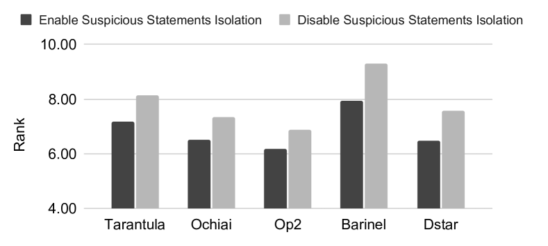
Figure 6: Impact of Buggy PC Detection on performance

Interestingly, even when disabling Suspicious Statements Isolation, this variant of VarCop is still better than S-SBFL and SBFL. Specially, VarCop obtained a better Rank than S-SBFL and SBFL in 21/30 and 27/30 metrics, respectively. In these ranking metrics, the average improvements of VarCop compared to S-SBFL and SBFL are 34% and 45%. Meanwhile, for the remaining metrics, the performances of S-SBFL and SBFL are better than VarCop by only 10% and 3%. For the bug in Fig. 3, thanks to the proposed suspiciousness measurement approach, this variant of VarCop still ranked the buggy statement ($s_{3}$) $1^{st}$ which is much better than the $9^{th}$ and $10^{th}$ positions by S-SBFL and SBFL.

Note that, for 19/338 cases which possibly contain non-variability bugs (mentioned in Section 8.1), there might be no Buggy PC in these buggy systems to be detected. Moreover, the low-quality test suites in some passing (yet buggy) products might “fool" fault localization techniques [46]. These passing products might also make VarCop less effective in isolating suspicious statements. Hence, for these cases, we turn off VarCop’s suspicious statements isolation component to guarantee its effectiveness.

9.2.2 Impact of Ranking Metric on Performance

We also studied the impact of the selection of the local ranking metric on VarCop’s performance. To do that, we built different variants of VarCop with different metrics. In Table III (the $3^{rd}$ and $7^{th}$ columns), the performance of VarCop is quite stable with the different ranking metrics. Particularly, for all the studied metrics, the average EXAM achieved by VarCop is in a narrow range, from 1.71–3.58, with the standard deviation of 0.46. Additionally, the average Rank of the buggy statements assigned by VarCop is varied from $6^{th}$–$14^{th}$. This stability of VarCop is obtained due to the suspicious statements isolation and suspiciousness measurement components. Indeed, VarCop only considers the statements that are related to the interactions which are the root causes of the failures. Moreover, VarCop is not biased by the test suites of any specific products. Consequently, its performance is less affected by the low-quality test suites of any product. Thus, selecting an inappropriate ranking metric, which is unknown beforehand in practice, does not significantly affect VarCop’s performance. This demonstrates that VarCop is practical in localizing variability bugs.

In contrast, the performances of S-SBFL and SBFL techniques are considerably impacted by choosing the ranking metrics. By S-SBFL method, the average Rank of the buggy statements widely fluctuates from $6^{th}$ to $28^{th}$. By SBFL, the fluctuation of Rank is even much more considerable, from $7^{th}$ to $243^{rd}$. Consequently, the QA process would be extremely inefficient if developers using the SBFL technique with an inappropriate ranking metric.

9.2.3 Impact of Normalization on Performance

To study the impact of the normalization, we built the variants of VarCop which enable and disable the normalization component. In this experiment, in both cases, the local test case-based scores are accordingly measured by 30 popular SBFL metrics and are aggregated by arithmetic mean.

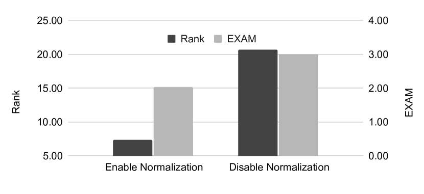
Figure 7: Impact of Normalization on performance

In Fig. 7, when enabling the normalization, VarCop’s performance is better than when normalization is off. Particularly, the performance of VarCop is improved 64% in Rank and 32% in EXAM when the normalization is enabled. One reason is that for some SBFL metrics, such as Fleiss [47] and Humman [48], the ranges of the product-based and test case-based suspiciousness values are significantly different. Additionally, for these metrics, the ranges of the local test case-based suspiciousness scores in different products are also significantly different. For example, there is a bug (ID_25) in the system Email, with Fleiss, the range of suspiciousness scores in product $p_{1}$ is $[-33,1.8]$, while the range in another product, $p_{2}$ is much different, $[-8.6,1.78]$. Without normalization, a statement in $p_{2}$ is more likely to be assigned a higher final score than one in $p_{1}$. Meanwhile, with several metrics such as Ochiai [41] and Tarantula [40], the performance of VarCop is slightly different when normalization is on/off. For these metrics, the local scores of the statements in the products are originally assigned in quite similar ranges. Thus, these local scores might not need to be additionally normalized. Overall, to ensure that the best performance of VarCop, the normalization should be on.

9.2.4 Impact of Aggregation Function on Performance

To study the impact of choosing aggregation function on performance, we varied the aggregation function of the test case-based suspiciousness assessment. In this experiment, Op2 [33] was randomly chosen to measure the local scores of the statements. As seen in Fig. 8, the performance of VarCop is not significantly affected when the aggregation function is changed. Specially, the average Rank of VarCop is around $6^{th}-7^{th}$, while the EXAM is about 1.76.

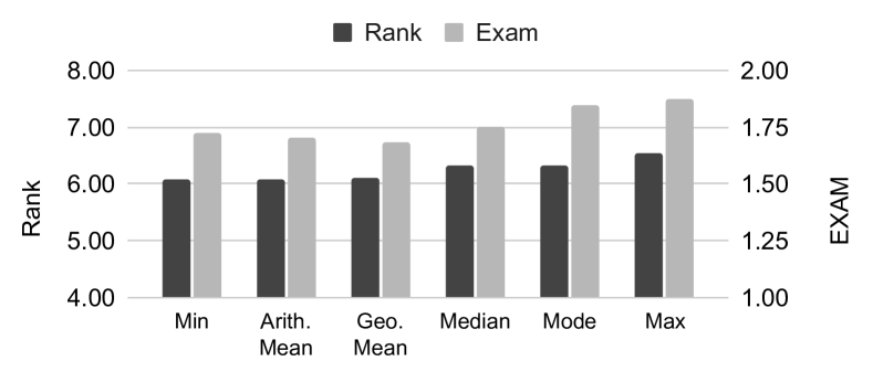
Figure 8: Impact of choosing $score(s,M)$ on performance

9.2.5 Impact of Combination Weight on Performance

Figure 9: Impact of choosing combination weight on performance

We varied the combination weight $w\in[0,1]$ (Section 7) when combining the product-based and test case-based suspiciousness assessments to form the final score of statements. Fig. 9 shows the average Rank and EXAM of the faults in 36 buggy versions of Email, with $w\in[0,1]$.

As seen, the performance of VarCop is better when both the product-based and test case-based suspiciousness scores are combined to measure the suspiciousness of the statements. For $w=1$, the statements are ranked by only their product-based suspiciousness. All the statements in the same feature will have the same suspiciousness score because they appear in the same number of passing and failing products. For $w=0$, a statement is ranked by only the score which is aggregated from the local scores of the statement in the failing products. Consequently, the overall performance may be affected by the low-quality test suites of some products. For instance, the correct statement $s$ appears in only one failing product $p$. However, in $p$, $s$ is misleadingly assigned the highest score. As a result, when $w=0$, $s$ also has the highest score in the whole system, since this score is aggregated from $p$, the only failing product containing $s$. Hence, both of the product-based and test case-based suspiciousness assessments are necessary for measuring the suspiciousness of statements (Mentioned in O3).

9.3 Sensitivity Analysis (RQ3)

9.3.1 Impact of Sample Size on Performance

In this experiment, for each buggy version of GPL which is randomly selected system, we used $k$-wise coverage, for $k\in[1,4]$, to systematically vary sample size. Then, we ran VarCop on each case with each set of sampled products.

Fig. 10 shows the average Rank and EXAM of VarCop in the buggy versions of GPL with different sample sets. As expected, the larger sample, the higher performance in localizing bugs obtained by VarCop. However, when the ranking results reach a specific point, even more products are tested, the results are just slightly better. Specially, for the set of $1$-wise coverage (One-disabled [5]), the average Rank and EXAM are about 4.31 and 0.45, respectively. Meanwhile, for $2$-wise, the ranking results are 1.5 times better. The reason is that, for a case, the more products are tested, the more information VarCop has to detect Buggy PCs and rank suspicious statements. However, compared to 3-wise and 4-wise, even much more products are sampled, which is much more costly in sampling and testing, the performance is just slightly improved. Hence, with VarCop, one might not need to use a very large sample to achieve a relatively good performance in localizing variability bugs.

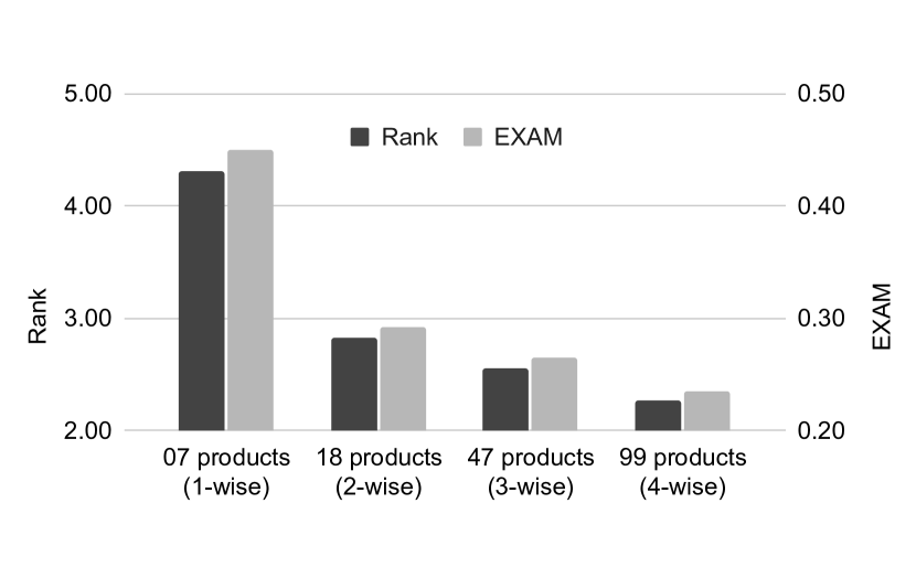
Figure 10: Impact of the sample size on performance

9.3.2 Impact of Test Suite’s Size on Performance

In this experiment, for every buggy version, we gradually increased the size of the test suite in each product to study the impact of tests on VarCop’s performance. The randomly selected system in this experiment is ExamDB.

In Fig. 11, VarCop’s performance is improved when increasing the test suite size. Particularly, when the number of tests increased from 13 to 90 tests/product, both Rank and EXAM of VarCop are improved by about twice. After that, even more tests are added, VarCop’s performance is just slightly affected. The reason is, increasing the number of tests provides more information to distinct the correct and incorrect statements, thus improves VarCop’s performance. However, when the test suites reach a specific effectiveness degree in detecting bugs, added tests would not provide supplementary information for the FL process.

Figure 11: Impact of the size of test set on performance

Overall, one should trade off between the fault localization effectiveness and the cost of generating tests and running them. Furthermore, as discussed in Section 9.2.1, instead of focusing on expanding test suites for products, developers should improve the effectiveness of the test suites in detecting bugs. This can be done by improving test coverage and applying mutation testing [49].

9.4 Performance in Localizing Multiple Bugs (RQ4)

To evaluate VarCop on buggy systems that contain multiple variability bugs, we conducted an experiment on 1,232 buggy versions of the subject systems with 2,947 variability bugs in total. The components of VarCop were randomly configured: the ranking metric is Op2 [33], and the aggregation function is arithmetic mean. For other settings of VarCop, one can find on our website [39].

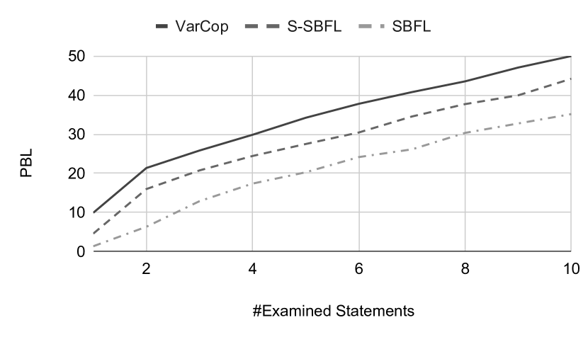
Figure 12: VarCop, S-SBFL and SBFL in localizing multiple bugs

Fig. 12 shows that the average percentage of buggy statements in each case found (PBL) by VarCop far surpasses the corresponding figures of S-SBFL and SBFL when the same number of statements are examined in their ranked lists. Specially, after examining the first statement, VarCop can find nearly 10% of the incorrect statements in a buggy system. Meanwhile, only 5% and 1% of the bugs are found by S-SBFL and SBFL, respectively, after inspecting the first statement. Furthermore, about 35% of the bugs can be found by VarCop by checking only first 5 statements in the ranked lists. Meanwhile, with S-SBFL and SBFL, developers have to investigate up to 7 and even 10 statements to achieve the same performance. In addition, the average best Rank that VarCop assigned for the buggy statements is about $7^{th}$. Meanwhile, the corresponding figures of S-SBFL, SBFL, and Arrieta et al. [10] are $7.5^{th}$, $10^{th}$, and $293^{th}$, respectively.

Especially, in 22% of the cases, VarCop correctly ranked at least one of the bugs at the top-1 positions, while for S-SBFL, SBFL, and Arrieta et al. [10], the corresponding proportions are only 10%, 3%, and 0%. In our experiment, at least one of the buggy statements of about 65% of cases are correctly ranked at top-5 positions by VarCop.

Fig. 13 shows a case (ID_143) containing two buggy statements in GPL. For the bug in Fig. 13 (13(a)), VarCop correctly ranked it $1^{st}$. Since in practice, the number of incorrect statements is unknown beforehand, developers have to conduct the testing and debugging processes in regression. After fixing the first bug, developers have to perform regression testing. One more time, VarCop effectively ranked the bug in Fig. 13 (13(b)) at the $2^{nd}$ position. Thus, developers can continuously use VarCop in the regression process to quickly find all the bugs in the systems. Meanwhile, by using SBFL, two buggy statements are ranked $4^{th}$ and $5^{th}$, respectively. This shows the effectiveness of VarCop in localizing multiple variability bugs in SPL systems.

⬇

1public void preVisitAction(Vertex v){

2 if (v.visited != true) {

3 v.VertexNumber = --vertexCounter;

4 //Patch: v.VertexNumber = vertexCounter++;

5 }

6}

(a) A variability bug in feature Number

⬇

1public void addEdge( Vertex start, Neighbor theNeighbor){

2 original( start, theNeighbor );

3 if (isDirected != false) {

4 //Patch: isDirected == false

5 Vertex end = theNeighbor.neighbor;

6 end.addWeight( end, theNeighbor.weight );

7 }

8}

(b) Another variability bug in WeightedWithNeighbors

Figure 13: A case of multiple bugs in GPL

9.5 Time complexity (RQ5)

We conducted our experiments on a desktop with Intel Core i5 2.7GHz, 8GB RAM. In 65% of the cases, VarCop took only about 2 minutes to automatically localize buggy statements in each case. On average, VarCop spent about 20 minutes on a buggy SPL system. Furthermore, we study VarCop’s running time in different input aspects including the sample size and the complexity of buggy systems in LOCs. For details, see our website [39].

Particularly, the running time of VarCop gracefully increased when we used more products to localize bugs (no show). This is expected because to localize the variability bugs, VarCop needs to examine the configurations of the more sampled products to detect Buggy PCs. Additionally, VarCop analyzes the detected Buggy PCs in these products to isolate the suspicious statements. Then calculating their suspiciousness scores, as well as ranking these statements.

For the complexity of buggy systems, in general, VarCop took more time to analyze the system which has more lines of code (no show). In particular, VarCop took the least time to localize bugs in the smallest system, BankAccountTP, while it took more time to investigate a case in the larger one, ZipMe. However, VarCop needs more time to investigate a case in Email compared to a case in ExamDB, which is larger than Email in terms of LOC. The reason is, VarCop analyzes all the failing products to isolate suspicious statements. In our experiment, there are many cases where the number of failing products in Email is larger than the number of failing products in ExamDB.

9.6 Threats to Validity

The main threats to the validity of our work are consisted of three parts: internal, construct, and external validity threat.

Threats to internal validity mainly lie in the correctness of the implementation of our approach. To reduce this threat, we manually reviewed our code [39] and verified our program analysis tools’ outputs.

Threats to construct validity mainly lie in the rationality of the assessment metrics. To reduce this threat, we chose the metrics that have been recommended by prior studies/surveys [15] and widely used in previous work [14, 11].

Threats to external validity mainly lie in the benchmark used in our experiments. The artificial bugs are generated by the mutation testing tool, this will make the diversity of artificial faults in the benchmark, yet could also introduce a bias in our evaluation. To reduce this threat, our experiments are conducted on various kinds of mutation operators on both single-bug and multiple-bug settings.

In addition, there is also a threat to external validity is that the obtained results on artificial faults can not be generalized for large-scale SPL systems containing real faults. To mitigate the threat, we chose six widely-used systems in existing studies [4, 8, 50], which target different application domains, and obtained consistent results on these systems. Moreover, although it has been very common to evaluate and compare fault localization techniques using artificial faults as a proxy to real faults [11], it remains an open question whether results on artificial faults are characteristic of results on real faults. In future work, we are planning to create manually-seeded faults and collect more real-world variability bugs in larger SPL systems to evaluate our technique to address these threats. As another external threat, all systems in the benchmark are developed in Java. Therefore, we cannot claim that similar results would have been observed in other programming languages or technologies. This is a common threat of several studies on configurable software systems [51, 52].

Another threat is that our selected SBFL metrics might not be representative. To reduce the threat, we chose a large number of the most popular SBFL metrics [14, 15, 11].

10 Related Work

Fault Localization. There are various approaches proposed to identify the locations of faults in programs [9, 53, 54, 55]. Program slicing [12, 13] is used in many studies to reduce the search space while localizing bugs by deleting irrelevant parts in code. Both static slicing [53, 54] and dynamic slicing [56, 55] are used to aid programmers in finding defects. In addition, by SBFL, a program spectrum, which records the execution information of a program, can be used to localize bugs. This idea was suggested by Collofello and Cousins [57]. To calculate suspiciousness, in early studies [58, 59], only information of failed tests was used. In later studies [17, 60, 27], which are better, both of the passed and failed tests are utilized. Moreover, several studies [21, 22] have shown that the FL performance is improved by combining SBFL technique with slicing methods. In comparison, while these techniques are designed to localize bugs in a particular product and cannot be directly applied for variability bugs, VarCop is specialized for variability bugs in SPL systems.

VarCop is closely related to the work by Arrieta et al. [10]. They use SBFL metrics to localize bugs at the feature-level and then create valid products of minimum size containing the most suspicious features. That approach focuses on identifying buggy features where all the containing statements are considered equally suspicious, while VarCop is designed to localize variability bugs in the statement-level.

Feature Interaction. There are a large number of approaches to investigate feature interactions as the influences of the features on the others’ behaviors in an unexpected way [25, 3]. Depending on the level of granularity and purposes, various approaches were proposed to detect feature interactions. In black-box fashion, Siegmund et al. [61] detects interactions to predict system performance by analyzing the influences of the selected features on the others’ non-functional properties. Based on the specifications, model checking is also used to check whether the combined features hold the specified properties [62, 63]. In several studies [7, 64, 30], interactions are detected by analyzing code. Nguyen et al. [7] detect interactions based on their shared program entities. In other studies [64, 30], they leverage control and data flow analyses to identify the interactions among features. iGen [65] employs an iterative method that runs the system, captures coverage data, processes data to infer interactions, and then creates new products to further refine interactions in the next iteration. In VarCop, feature interactions are detected for the purpose of identifying statements which suspiciously cause the failures. We detect not only interactions of enabled features but also disabled features, which are the root causes of the failures of the systems. For a set of enabled features, their interaction is detected by their influences on the other’s implementation via control and data dependency. For disabled features, their impacts are estimated by the shared program entities.

Variability Bugs. Variability bugs are complex and difficult to be detected by both humans and tools because they involve multiple system features and only be revealed in certain products [5, 23, 3, 31]. Abal et al. [5, 23] analyzed the real variability bugs in several large highly-configurable systems such as Linux kernel and Busybox to understand the complexity and the nature of this kind of bugs. In order to make a white-box understanding of interaction faults, Garvin et al. [3] presented the criteria for interaction faults to be present in systems. Their criteria are about the statements whose (non-)execution is necessary for the failure to be exposed/masked.

Quality Assurance for Configurable Code There are various studies about variability-aware analysis for the purpose of type checking [66, 67], testing [68, 51], and control/data flow analysis[69, 67]. In addition, to improve the efficiency of the QA process, several approaches about configuration selection [70, 71] and configuration prioritization [7, 72] have been proposed.

11 Conclusion

We introduce VarCop, a novel approach for localizing variability bugs. First, to isolate the suspicious statements, VarCop analyzes the overall test results and the failing products’ code to detect the statements related to the interactions that potentially make the bugs (in)visible in the products. Then, VarCop ranks each isolated statement based on two suspiciousness dimensions which are measured by both the overall test results of the products and the detailed results of the test cases which are executed by the statement. We conducted several experiments on a large dataset of buggy versions of 6 SPL systems in both single-bug and multiple-bug settings. Our results show that in the all 30/30 most popular ranking metrics, VarCop’s performance in Rank is 33%, 50% and 95% better than the state-of-the-art FL techniques, S-SBFL, SBFL, and Arrieta et al. [10], for single-bug cases. Moreover, VarCop correctly ranked the buggy statement in +65% of the cases at the top-3 positions in the resulting lists. For the cases of multiple-bug, one-third of the bugs in a buggy system are ranked at top-5 positions by VarCop. Especially, in 22% and 65% of the cases, VarCop is able to effectively localize at least one buggy statement at top-1 and top-5 positions of its ranked lists, respectively. From that, developers can iterate the process of bugs detecting, bugs fixing, and regression testing to quickly fix all the bugs and assure the quality of SPL systems.

Thu-Trang Nguyen is a Ph.D. candidate in Software Engineering at University of Engineering and Technology, Vietnam National University, Hanoi (VNU - UET). She received her MSc degree from Japan Advanced Institute of Science and Technology in 2019 and received her BSc degree from VNU - UET in 2016. Her research interests include program analysis, software product line systems, software vulnerabilities detection, and software testing.

Kien-Tuan Ngo earned the Bachelor’s degree from VNU University of Technology and Engineering, Vietnam in 2020. After that, he continues to work as a full-time researcher at the Faculty of Information Technology at the same college. His research interests include source code analysis, software testing, machine learning for code, and empirical software engineering.

Son Nguyen is a Ph.D. Candidate in Computer Science at the University of Texas at Dallas. He received the BSc degree in Computer Science from Vietnam National University, Hanoi, in 2015. His research interests include program analysis, configurable code analysis, and statistical approaches in software engineering.

Hieu Dinh Vo is the head of the Department of Software Engineering at the Faculty of Information Technology, the University of Engineering and Technology, VNU Hanoi. He earned a Bachelor’s degree in Computer Engineering from the Ho Chi Minh City University of Technology, a Master’s degree in Distributed Multimedia Systems from the University of Leeds, and a Ph.D. in Information Science from the Japan Advanced Institute of Science and Technology. His research interests include source code analysis, software testing, service computing, and software architecture.

References

- [1] S. Apel, D. Batory, C. Kästner, and G. Saake, Feature-Oriented Software Product Lines: Concepts and Implementation. Springer Publishing Company, Incorporated, 2013.
- [2] S. Apel, D. Batory, C. Kästner, and G. Saake, Feature-oriented software product lines. Springer, 2016.
- [3] B. J. Garvin and M. B. Cohen, “Feature interaction faults revisited: An exploratory study,” in 2011 IEEE 22nd International Symposium on Software Reliability Engineering. IEEE, 2011, pp. 90–99.
- [4] S. Apel, A. Von Rhein, P. Wendler, A. Größlinger, and D. Beyer, “Strategies for product-line verification: case studies and experiments,” in 2013 35th International Conference on Software Engineering (ICSE). IEEE, 2013, pp. 482–491.
- [5] I. Abal, C. Brabrand, and A. Wasowski, “42 variability bugs in the linux kernel: a qualitative analysis,” in Proceedings of the 29th ACM/IEEE international conference on Automated software engineering, 2014, pp. 421–432.
- [6] F. Medeiros, C. Kästner, M. Ribeiro, R. Gheyi, and S. Apel, “A comparison of 10 sampling algorithms for configurable systems,” in 2016 IEEE/ACM 38th International Conference on Software Engineering (ICSE). IEEE, 2016, pp. 643–654.
- [7] S. Nguyen, H. Nguyen, N. Tran, H. Tran, and T. Nguyen, “Feature-interaction aware configuration prioritization for configurable code,” in 2019 34th IEEE/ACM International Conference on Automated Software Engineering (ASE). IEEE, 2019, pp. 489–501.
- [8] J. Meinicke, C.-P. Wong, C. Kästner, T. Thüm, and G. Saake, “On essential configuration complexity: measuring interactions in highly-configurable systems,” in Proceedings of the 31st IEEE/ACM International Conference on Automated Software Engineering, 2016, pp. 483–494.
- [9] W. E. Wong, R. Gao, Y. Li, R. Abreu, and F. Wotawa, “A survey on software fault localization,” IEEE Transactions on Software Engineering, vol. 42, no. 8, pp. 707–740, 2016.
- [10] A. Arrieta, S. Segura, U. Markiegi, G. Sagardui, and L. Etxeberria, “Spectrum-based fault localization in software product lines,” Information and Software Technology, vol. 100, pp. 18–31, 2018.
- [11] S. Pearson, J. Campos, R. Just, G. Fraser, R. Abreu, M. D. Ernst, D. Pang, and B. Keller, “Evaluating and improving fault localization,” in 2017 IEEE/ACM 39th International Conference on Software Engineering (ICSE). IEEE, 2017, pp. 609–620.
- [12] M. Weiser, “Program slicing,” IEEE Transactions on software engineering, no. 4, pp. 352–357, 1984.
- [13] H. Agrawal and J. R. Horgan, “Dynamic program slicing,” ACM SIGPlan Notices, vol. 25, no. 6, pp. 246–256, 1990.
- [14] F. Keller, L. Grunske, S. Heiden, A. Filieri, A. van Hoorn, and D. Lo, “A critical evaluation of spectrum-based fault localization techniques on a large-scale software system,” in 2017 IEEE International Conference on Software Quality, Reliability and Security (QRS). IEEE, 2017, pp. 114–125.
- [15] L. Naish, H. J. Lee, and K. Ramamohanarao, “A model for spectra-based software diagnosis,” ACM Transactions on software engineering and methodology (TOSEM), vol. 20, no. 3, pp. 1–32, 2011.
- [16] R. Abreu, P. Zoeteweij, and A. J. Van Gemund, “Spectrum-based multiple fault localization,” in 2009 IEEE/ACM International Conference on Automated Software Engineering. IEEE, 2009, pp. 88–99.
- [17] R. Abreu, P. Zoeteweij, and A. J. van Gemund, “On the accuracy of spectrum-based fault localization,” in Testing: Academic and Industrial Conference Practice and Research Techniques - MUTATION (TAICPART-MUTATION 2007), 2007, pp. 89–98.
- [18] K.-T. Ngo, T.-T. Nguyen, S. Nguyen, and H. D. Vo, “Variability fault localization: A benchmark,” in Proceedings of the 25th ACM International Systems and Software Product Line Conference - Volume A, ser. SPLC ’21, 2021, p. 120–125.
- [19] I. do Carmo Machado, J. D. McGregor, and E. Santana de Almeida, “Strategies for testing products in software product lines,” ACM SIGSOFT Software Engineering Notes, vol. 37, no. 6, pp. 1–8, 2012.
- [20] T. Thüm, S. Apel, C. Kästner, I. Schaefer, and G. Saake, “A classification and survey of analysis strategies for software product lines,” ACM Computing Surveys (CSUR), vol. 47, no. 1, pp. 1–45, 2014.
- [21] N. B. Chaleshtari and S. Parsa, “Smbfl: slice-based cost reduction of mutation-based fault localization,” Empirical Software Engineering, vol. 25, no. 5, pp. 4282–4314, 2020.
- [22] X. Li and A. Orso, “More accurate dynamic slicing for better supporting software debugging,” in 2020 IEEE 13th International Conference on Software Testing, Validation and Verification (ICST). IEEE, 2020, pp. 28–38.
- [23] I. Abal, J. Melo, Ş. Stănciulescu, C. Brabrand, M. Ribeiro, and A. Wąsowski, “Variability bugs in highly configurable systems: A qualitative analysis,” ACM Transactions on Software Engineering and Methodology (TOSEM), vol. 26, no. 3, pp. 1–34, 2018.
- [24] A. Mordahl, J. Oh, U. Koc, S. Wei, and P. Gazzillo, “An empirical study of real-world variability bugs detected by variability-oblivious tools,” in Proceedings of the 2019 27th ACM Joint Meeting on European Software Engineering Conference and Symposium on the Foundations of Software Engineering, 2019, pp. 50–61.
- [25] S. Apel, S. Kolesnikov, N. Siegmund, C. Kästner, and B. Garvin, “Exploring feature interactions in the wild: the new feature-interaction challenge,” in Proceedings of the 5th International Workshop on Feature-Oriented Software Development, 2013, pp. 1–8.
- [26] IEEE, “Ieee standard glossary of software engineering terminology,” IEEE Std 610.12-1990, pp. 1–84, 1990.
- [27] M. Zhang, X. Li, L. Zhang, and S. Khurshid, “Boosting spectrum-based fault localization using pagerank,” in Proceedings of the 26th ACM SIGSOFT International Symposium on Software Testing and Analysis, 2017, pp. 261–272.
- [28] M. Wen, J. Chen, Y. Tian, R. Wu, D. Hao, S. Han, and S.-C. Cheung, “Historical spectrum based fault localization,” IEEE Transactions on Software Engineering, 2019.
- [29] M. J. Harrold, G. Rothermel, R. Wu, and L. Yi, “An empirical investigation of program spectra,” in Proceedings of the 1998 ACM SIGPLAN-SIGSOFT workshop on Program analysis for software tools and engineering, 1998, pp. 83–90.
- [30] L. R. Soares, J. Meinicke, S. Nadi, C. Kästner, and E. S. de Almeida, “Varxplorer: Lightweight process for dynamic analysis of feature interactions,” in Proceedings of the 12th International Workshop on Variability Modelling of Software-Intensive Systems, 2018, pp. 59–66.
- [31] D. R. Kuhn, D. R. Wallace, and A. M. Gallo, “Software fault interactions and implications for software testing,” IEEE transactions on software engineering, vol. 30, no. 6, pp. 418–421, 2004.
- [32] L. Bian and R. Butler, “Comparing effects of aggregation methods on statistical and spatial properties of simulated spatial data,” Photogrammetric engineering and remote sensing, vol. 65, pp. 73–84, 1999.
- [33] H. Ding, L. Chen, J. Qian, L. Xu, and B. Xu, “Fault localization method using information quantity,” Ruan Jian Xue Bao/Journal of Software, vol. 24, no. 7, pp. 1484–1494, 2013.
- [34] W. E. Wong, V. Debroy, R. Gao, and Y. Li, “The dstar method for effective software fault localization,” IEEE Transactions on Reliability, vol. 63, no. 1, pp. 290–308, 2013.
- [35] M. F. Johansen, Ø. Haugen, and F. Fleurey, “An algorithm for generating t-wise covering arrays from large feature models,” in Proceedings of the 16th International Software Product Line Conference-Volume 1, 2012, pp. 46–55.
- [36] E. Wong, T. Wei, Y. Qi, and L. Zhao, “A crosstab-based statistical method for effective fault localization,” in 2008 1st international conference on software testing, verification, and validation. IEEE, 2008, pp. 42–51.
- [37] L. Lucia, D. Lo, and X. Xia, “Fusion fault localizers,” in Proceedings of the 29th ACM/IEEE international conference on Automated software engineering, 2014, pp. 127–138.
- [38] C. Parnin and A. Orso, “Are automated debugging techniques actually helping programmers?” in Proceedings of the 2011 international symposium on software testing and analysis, 2011, pp. 199–209.
- [39] [Online]. Available: https://ttrangnguyen.github.io/VARCOP/
- [40] J. A. Jones, M. J. Harrold, and J. Stasko, “Visualization of test information to assist fault localization,” in Proceedings of the 24th International Conference on Software Engineering. ICSE 2002. IEEE, 2002, pp. 467–477.
- [41] A. Ochiai, “Zoogeographic studies on the soleoid fishes found in japan and its neighbouring regions,” Bulletin of Japanese Society of Scientific Fisheries, vol. 22, pp. 526–530, 1957.
- [42] A. d. S. Meyer, A. A. F. Garcia, A. P. d. Souza, and C. L. d. Souza Jr, “Comparison of similarity coefficients used for cluster analysis with dominant markers in maize (zea mays l),” Genetics and Molecular Biology, vol. 27, no. 1, pp. 83–91, 2004.
- [43] Y.-S. Ma, J. Offutt, and Y.-R. Kwon, “Mujava: a mutation system for java,” in Proceedings of the 28th international conference on Software engineering, 2006, pp. 827–830.
- [44] V. Sobreira, T. Durieux, F. Madeiral, M. Monperrus, and M. de Almeida Maia, “Dissection of a bug dataset: Anatomy of 395 patches from defects4j,” in 2018 IEEE 25th International Conference on Software Analysis, Evolution and Reengineering (SANER). IEEE, 2018, pp. 130–140.
- [45] B. H. Smith and L. Williams, “On guiding the augmentation of an automated test suite via mutation analysis,” Empirical software engineering, vol. 14, no. 3, pp. 341–369, 2009.
- [46] B. Baudry, F. Fleurey, and Y. Le Traon, “Improving test suites for efficient fault localization,” in Proceedings of the 28th international conference on Software engineering, 2006, pp. 82–91.
- [47] J. L. Fleiss, “Estimating the accuracy of dichotomous judgments,” Psychometrika, vol. 30, no. 4, pp. 469–479, 1965.
- [48] F. Lourenço, V. Lobo, and F. Bacao, “Binary-based similarity measures for categorical data and their application in self-organizing maps,” 2004.
- [49] M. Papadakis, M. Kintis, J. Zhang, Y. Jia, Y. Le Traon, and M. Harman, “Mutation testing advances: an analysis and survey,” in Advances in Computers. Elsevier, 2019, vol. 112, pp. 275–378.
- [50] S. Apel, C. Kästner, and C. Lengauer, “Language-independent and automated software composition: The featurehouse experience,” IEEE Transactions on Software Engineering, vol. 39, no. 1, pp. 63–79, 2011.
- [51] C.-P. Wong, J. Meinicke, L. Lazarek, and C. Kästner, “Faster variational execution with transparent bytecode transformation,” Proceedings of the ACM on Programming Languages, vol. 2, no. OOPSLA, pp. 1–30, 2018.
- [52] S. Souto, M. d’Amorim, and R. Gheyi, “Balancing soundness and efficiency for practical testing of configurable systems,” in 2017 IEEE/ACM 39th International Conference on Software Engineering (ICSE). IEEE, 2017, pp. 632–642.
- [53] S. Kusumoto, A. Nishimatsu, K. Nishie, and K. Inoue, “Experimental evaluation of program slicing for fault localization,” Empirical Software Engineering, vol. 7, no. 1, pp. 49–76, 2002.
- [54] F. Tip and T. Dinesh, “A slicing-based approach for locating type errors,” ACM Transactions on Software Engineering and Methodology (TOSEM), vol. 10, no. 1, pp. 5–55, 2001.
- [55] R. A. DeMillo, H. Pan, and E. H. Spafford, “Critical slicing for software fault localization,” ACM SIGSOFT Software Engineering Notes, vol. 21, no. 3, pp. 121–134, 1996.
- [56] E. Alves, M. Gligoric, V. Jagannath, and M. d’Amorim, “Fault-localization using dynamic slicing and change impact analysis,” in 2011 26th IEEE/ACM International Conference on Automated Software Engineering (ASE 2011). IEEE, 2011, pp. 520–523.
- [57] J. S. Collofello and L. Cousins, “Towards automatic software fault location through decision-to-decision path analysis,” in Managing Requirements Knowledge, International Workshop on, 1987, pp. 539–539.
- [58] H. Agrawal, R. A. De Millo, and E. H. Spafford, “An execution-backtracking approach to debugging,” IEEE Software, vol. 8, no. 3, pp. 21–26, 1991.
- [59] B. Korel, “Pelas-program error-locating assistant system,” IEEE Transactions on Software Engineering, vol. 14, no. 9, pp. 1253–1260, 1988.
- [60] W. E. Wong, V. Debroy, and B. Choi, “A family of code coverage-based heuristics for effective fault localization,” Journal of Systems and Software, vol. 83, no. 2, pp. 188–208, 2010.
- [61] N. Siegmund, S. S. Kolesnikov, C. Kästner, S. Apel, D. Batory, M. Rosenmüller, and G. Saake, “Predicting performance via automated feature-interaction detection,” in 2012 34th International Conference on Software Engineering (ICSE). IEEE, 2012, pp. 167–177.
- [62] S. Apel, A. Von Rhein, T. ThüM, and C. KäStner, “Feature-interaction detection based on feature-based specifications,” Computer Networks, vol. 57, no. 12, pp. 2399–2409, 2013.
- [63] M. Calder and A. Miller, “Feature interaction detection by pairwise analysis of ltl properties—a case study,” Formal Methods in System Design, vol. 28, no. 3, pp. 213–261, 2006.
- [64] F. Angerer, A. Grimmer, H. Prähofer, and P. Grünbacher, “Configuration-aware change impact analysis (t),” in 2015 30th IEEE/ACM International Conference on Automated Software Engineering (ASE). IEEE, 2015, pp. 385–395.
- [65] T. Nguyen, U. Koc, J. Cheng, J. S. Foster, and A. A. Porter, “igen: Dynamic interaction inference for configurable software,” in Proceedings of the 2016 24th ACM SIGSOFT International Symposium on Foundations of Software Engineering, 2016, pp. 655–665.
- [66] C. Kästner, S. Apel, T. Thüm, and G. Saake, “Type checking annotation-based product lines,” ACM Transactions on Software Engineering and Methodology, vol. 21, no. 3, pp. 1–39, 2012.
- [67] J. Liebig, A. Von Rhein, C. Kästner, S. Apel, J. Dörre, and C. Lengauer, “Scalable analysis of variable software,” in Proceedings of the 2013 9th Joint Meeting on Foundations of Software Engineering, 2013, pp. 81–91.
- [68] L. R. Soares, J. Meinicke, S. Nadi, C. Kästner, and E. S. de Almeida, “Exploring feature interactions without specifications: A controlled experiment,” ACM SIGPLAN Notices, vol. 53, no. 9, pp. 40–52, 2018.
- [69] E. Bodden, T. Tolêdo, M. Ribeiro, C. Brabrand, P. Borba, and M. Mezini, “Spllift: Statically analyzing software product lines in minutes instead of years,” ACM SIGPLAN Notices, vol. 48, no. 6, pp. 355–364, 2013.
- [70] M. Greiler, A. van Deursen, and M.-A. Storey, “Test confessions: A study of testing practices for plug-in systems,” in 2012 34th International Conference on Software Engineering (ICSE). IEEE, 2012, pp. 244–254.
- [71] I. do Carmo Machado, J. D. McGregor, Y. C. Cavalcanti, and E. S. De Almeida, “On strategies for testing software product lines: A systematic literature review,” Information and Software Technology, vol. 56, no. 10, pp. 1183–1199, 2014.
- [72] M. Al-Hajjaji, T. Thüm, J. Meinicke, M. Lochau, and G. Saake, “Similarity-based prioritization in software product-line testing,” in Proceedings of the 18th International Software Product Line Conference-Volume 1, 2014, pp. 197–206.