Evolution of topics in central bank speech communication

Abstract

This paper studies the content of central bank speech communication from 1997 through 2020 and asks the following questions: (i) What global topics do central banks talk about? (ii) How do these topics evolve over time? I turn to natural language processing, and more specifically Dynamic Topic Models, to answer these questions. The analysis consists of an aggregate study of nine major central banks and a case study of the Federal Reserve, which allows for region specific control variables. I show that: (i) Central banks address a broad range of topics. (ii) The topics are well captured by Dynamic Topic Models. (iii) The global topics exhibit strong and significant autoregressive properties not easily explained by financial control variables.

JEL Classification: C38, C55, E52, E58
Keywords: Central bank communication, Monetary policy, Textual analysis, Dynamic topic models, Narratives

1 Introduction

I’m a weatherman, I’m a showman, and I’m an economist. I’m expected to be, and I am, a storyteller. I tell stories about the future. (Stefan Ingves, governor of the Swedish Riksbank)

Central bank communication affects financial markets [17, 15, 33] and makes monetary policy more predictable. Traditionally, central bank communication has had two primary functions: To reveal private information to the public, and to affect and coordinate financial market expectations [44, 1, 11]. This suggests that central bank communication should be focused on topics closely related to monetary policy. Is this really the case?

In this paper, I give a descriptive analysis of speeches by the major central banks connected to the Bank for International Settlements (BIS) and ask: (i) What global topics do central banks talk about? (ii) How do these topics evolve over time? In order to answer these questions I turn to natural language processing (NLP) to estimate the content of speeches from 9 major central banks using Dynamic Topic Models (DTM) [7].

The analysis shows that the central banks talk about a broad range of topics, not all related to classic theory of central bank communication. The estimated topics are persistent and exhibit a large significant autoregressive effect which is robust to different model specifications. To control for underlying variables, a case study using data from the Federal Reserve alone is conducted. The case study shows that topic persistence is not easily explained by controlling for regional financial variables related to the topics. This suggests that the topics exhibit what one might call a narrative effect, in which the topics are driven by economic narratives [41].

The body of research relating narratives to central bank communication is growing and there are evidence that narratives affect the economy [36, 25, 19]. These narratives could either be part of the global economy or created by the central banks themselves. This is also consistent with the concept of gradualism in which central banks tend to gradually change the interest rate rather than have large jumps. For instance, from 2001 to 2003 the Fed used gradualism to reduce the interest rate by 550 basis points over a sequence of thirteen cuts. Gradualism is founded on the theory of uncertainty in policy making, in which policymakers are inclined to gradually introduce a policy when its effect on the economy is ambiguous [13]. Similarly, central bank communication can introduce narratives that gradually prime the public for future policy changes, such as changes in financial market regulation or an introduction of central bank digital currency (CBDC). At present, many of the central banks are investigating a potential introduction of digital money and many of them are actively communicating on the matter through speeches and reports [4]. Thus, central banks are using verbal communication to inform and prepare the public for future structural change. This is an undocumented way for central banks to use communication in an active manner to make sure that monetary policy and regulatory changes are achieved as expected. This indicates that central bank speeches might address a broader range of topics than expected by the traditional view of central bank communication.

The two most common ways for central banks to communicate are: (i) Written disclosures of meeting minutes and reports. (ii) Speeches. Since the 1990s central bank communication strategies have undergone a transformation: Going from opaque secrecy, to greater transparency, to actively using communication as a tool for monetary policy [45, 11, 10]. One of these changes is a large increase in the number of speeches held in the overall communication strategies. This has led to a great growth in text data related to central banks, which now can be analyzed by recent machine learning techniques. Text data is multidimensional and rich in information. Using advances in computational linguistics, it is possible to reduce the dimensionality of the data and use it in economic analysis. The number of speeches from the central banks affiliated with the BIS, treated in this paper, was 119 in 1997, whereas in 2019 it was 423. Thus, the volume of the oral communication has increased greatly. Central bank speeches, in comparison to announcements, are richer in information, greater in number, significantly longer, and addresses a larger variety of topics. Therefore, speeches are ideal data to analyze the content of central bank communication.

Some research has previously been conducted analyzing central bank speeches. [28] show that speeches from the ECB affect the volatility of the euro-dollar exchange rate. [2] study speeches from the Swedish Riksbank and find that the speeches affect market prices, and that the market react stronger to communication from the head of the Riksbank. [12] show how sentiment of central bank speeches about financial stability have a significant effect on market returns and volatility. The two closest studies to this one, which also rely on topic modelling, are [24] and [3]. [24] study central bank transparency using topic modelling in an event study around 1993, the year the Fed started to release the FOMC meeting transcripts. [3] study spillover effects in sentiment from central bank speeches and show that cross-country effects affect both central bank communication as well as macroeconomic variables, where the Fed has a unique influence in creating sentiment spillover effects.

When the interest rate is close to the efficient lower bound (ELB), central bank communication is of increased importance, and forward guidance may be the main policy tool [11]. At these times, the public’s expectations of the central bank’s future policy is crucial, and indicates that central bank communication might be weighted towards forward guidance. Yet, the results of this paper suggest that the content of central bank communication is broad, also at times when the interest rates are close to the ELB. This is consistent with the research showing that the general public is either not targeted or affected by central bank communication [29, 30, 16], and the fact that trust in central banks is relatively low [26, 20]. [10] predicts that “central banks will keep trying to communicate with the general public, as they should, but for the most part, they will fail”. Drawing from the literature of narrative economics, [23] argue that effective communication needs to be simple, relevant, and story-based and that central bank communication fail at all three parts, making it inaccessible for the society in general.

This paper contributes to the literature in several ways. First, the paper provides a comprehensive dynamic analysis, not previously conducted, describing the evolution of the content of central bank communication. Second, the paper introduces the application of Dynamic Topic Models to the field of finance and economics. Third, I make inference about the autoregressive properties of the estimated topics, and show that there is strong persistence in the content, which is not explained by controlling for underlying financial variables. Finally, the paper draws connections between central bank communication, topic modelling, and narrative economics, yielding ideas for further improvements in central bank communication strategies, and suggestions on how topic modelling could be applied to narrative economics.

The rest of the paper is organized as follows: Section 2 describes the data; Section 3 outlines the methodology; Section 4 presents the main findings; in Section 5 a case study investigating the persistence of topics in speeches from the Federal Reserve is conducted, controlling for regional financial variables; and Section 6 concludes the paper.

2 Data

The central bank speech data was scraped from the BIS website. 14,423 central bank speeches were collected from 113 institutions, over the time period 1997 through 2020. The speeches consist of English sentences, meaning that the speeches are transcribed, and when needed translated, into only content and not including verbal sounds or utterances without meaning. This leads to a simpler preprocessing as the text does not contain dis-fluencies, such as fragments of words or filled pauses. [3] were first to use the BIS data source, using a shorter time period, and to my knowledge their paper is the only previous time the data source has been used.

The dataset was constrained to include global institutions with more than 200 speeches over the sample period. This criteria was chosen in order to select a sufficiently homogenous global and talkative subsample. Thus, local central bank branches, such as the Bank of Spain, were excluded from the dataset. The final data for the analysis consist of 7,379 speeches from 9 different central banks: Bank of Canada, Bank of England, Bank of Japan, Central Bank of Norway, ECB, Fed (including speeches from the New York Fed), Reserve Bank of Australia, Sweden’s Riksbank, and Swiss National Bank.

The preprocessing of the text data follows standard methodology [21]. The data were first transformed from pdf format to text format. Each document was split into lower case tokens (words), removing punctuation, numbers and web links. Headers and footers of the documents were removed, together with reference lists. A common list of stop words was applied to filter out words of little importance to the topic modelling. Through lemmatization the tokens were transformed into dictionary form, e.g., banks becoming bank. Bigrams, i.e, sequences of two adjacent tokens, and trigrams, i.e., sequences of three adjacent tokens, were created of commonly followed tokens, such as central bank and real interest rate. Extreme tokens, appearing less than 20 times in the corpus or in more than 50% of the documents, were also filtered out to reduce dimensionality and make interpretation simpler by avoiding topics to have the same top words in the generating distributions. Table 1 shows the data dimensionality reduction at each step in the preprocessing. After preprocessing, the data consist of 4,280,706 tokens and the vocabulary (alias dictionary) of 20,697 unique tokens.

	Raw text	Remove stopwords	Lemmatization	Bigrams and trigrams	Filter extremes
Total words	22,762,644	11,903,054	11,737,316	9,908,456	4,280,706
Unique words	66,735	58,478	53,116	65,282	20,697

Table 1: Data dimensionality reduction of each preprocessing step.

The control variables for the Fed case study were collected from the Wharton Research Data Service (WRDS). The data include: 1 year US treasury bond yields, US inflation, the S&P 500 Index returns, and the CBOE Volatility Index (VIX). The S&P 500 Index data and the VIX data have been down-sampled into quarterly observations by choosing the maximum values in each quarter. The maximum values were chosen to preserve as much of the variance in the data as possible.

3 Methodology

In order to analyze the central bank speech data, I use Dynamic Topic Models (DTM) [7] together with Autoregressive (AR) models. DTM has not, to my knowledge, previously been applied in the field of finance and economics. DTM let the topics dynamically change over time, meaning that the word distributions that define the topics are dynamic. This allows the researcher to study the time evolution of the latent dynamic topics discovered by the model. It also improves upon transparency when using the estimated topics in time series modelling, since the researcher can verify homogeneity of the topic distributions over time. One can thus identify whether a topic is about the same subject throughout the sample period.

Latent Dirichlet Allocation (LDA) [9] has become the standard topic model in the applied literature, building on Latent Semantic Indexing (LSI) introduced by [18], and later extended by [37] and [27]. These methods have become increasingly popular in finance and economics, for an overview of NLP in economics see [21]. Like the LDA model, DTM are a set of generative probabilistic models for discrete data, popular for text, that introduce a time dimension to the LDA framework and let topics evolve over time. The DTM are unsupervised and use a bag-of-words structure, meaning that the order of the words do not matter. However in contrast to the static LDA model, the order of the documents do matter. The dynamic model addresses the static assumption of the LDA model by updating the distributions parameters for each time slice, which in this paper is done annually. This is done by introducing a state space model using a logistic normal distribution. In the model, each document is generated from a mixture of topics and each topic is generated from a mixture of words from the vocabulary.

Given a model with $K$ topics, $D$ documents, and a vocabulary with $V$ terms, let $\beta_{t,k}$ be a $V$-dimensional vector representing topic $k$ at time $t$, where $t=1,\ldots,T$ and $k=1,\ldots,K$. $\beta_{t,k}$ evolves with a Gaussian random walk, $\beta_{k,t}|\beta_{k,t-1}\sim\mathcal{N}(\beta_{k,t-1},\sigma^{2}I)$, meaning that the word distribution over topics change over time. Furthermore, let $\alpha_{t}$ be a $D$-dimensional mean parameter vector of the logistic normal distribution for the topic proportions, following a Gaussian random walk, $\alpha_{t}|\alpha_{t-1}\sim\mathcal{N}(\alpha_{t-1},\delta^{2}I)$. A set of topic models are sequentially chained together and the generative process for time slice $t$ of a sequential corpus is as follows:

1. Draw topics distributions over dictionary $\beta_{k,t}|\beta_{k,t-1}\sim\mathcal{N}(\beta_{k,t-1},\sigma^{2}I)$.

2. Draw mean parameters of document distributions over topics $\alpha_{t}|\alpha_{t-1}\sim\mathcal{N}(\alpha_{t-1},\delta^{2}I)$.

3. For each document:

   1. Draw $\eta\sim\mathcal{N}(\alpha_{t},a^{2}I)$.

   2. For each word position $n\in N_{d}$:

      1. Draw topic $Z\sim Mult(\pi(\eta))$.

      2. Draw word $W_{t,d,n}\sim Mult(\pi(\beta_{t,z}))$.

Here $\pi(\beta_{k,t})_{w}=\frac{\exp(\beta_{k,t,w)}}{\sum\exp(\beta_{k,t,w)}}$ maps the multinomial natural parameters to the mean parameters. From a practical point of view, one does not generate the corpus, but rather backs out the underlying latent distributions, given a corpus, with variational Bayesian inference. The standard deviations of the Gaussian random walks are not estimated but set to a fixed value given by the implementation in [7], which is used in this paper together with a Python wrapper [38]. To not estimate these hyperparameters is standard in the literature but nevertheless a limitation of the methodology since it restricts to what degree the topics can change over time.

In a practical way the model can be understood to yield two kinds of results. First, the model outputs a set of $K$ $V$-dimensional topic distributions for each time slice $t$. These topic distributions are functions of the vocabulary and define the $K$ estimated topics in the model. In a topic’s probability distribution, each word in the vocabulary at each time slice is assigned a probability defining how likely that word is to be drawn from that topic at time $t$. Therefore, the most probable words of a topic’s distribution constitute the theme of that topic. The topic names are manually labelled by these themes. By tracking the changes in a topic’s distribution across time it is possible to study how the topic evolves. An example can be seen in Table 2 in Section 4.1 for the estimated topic about supervision and regulation. Second, with a trained model each document in the corpus can be assigned a static $K$-dimensional distribution of topics, where each topic is assigned a probability. This means that each document is classified with a set of topic probabilities describing how likely the document is to have been generated from each of the topics. By classifying the documents and averaging the distributions on a monthly or quarterly basis, it is possible to track the evolution of topics discussed in the documents over time, as seen in Figure 1 in Section 4.1. Thus, by the output of the model we are able to study both the evolution of topics discussed throughout the sample period, as well as the terminology-evolution of the topics’ distributions.

The progression of topics discussed and the within topic change are both functions of the underlying corpus. If certain significant global events are happening on the financial markets we would expect a topic about financial markets to include the contemporary relevant language and have a higher probability of being addressed. However, the emerging literature of narrative economics [41] suggests that there are additional variables affecting the development and spread of topics. Narrative economics can be an explaining theory of what is driving the unexplained persistence in the model. Narratives in the global economy, or narratives created by the central banks themselves, can be contributing factors to what words are likely to appear in the topics’ distributions in each time slice, as well as what topics are likely talked about in each time slice.

Choosing the number of topics, $K$, is a non trivial and highly researched area. In the DTM framework, the number of topics are assumed to be known, and therefore needs to be specified beforehand. A common way to determine the number of topics is to evaluate the model according to model perplexity [43] in which the inverse of the geometric mean of the per-word likelihood is evaluated. Another way is to evaluate the topic coherence, introduced by [35], which addresses the issue of human interpretability of the topics. If a topic is to make sense for humans, the top words contributing to the topic distribution needs to be semantically close to each other. This can be measured numerically with different coherence measures. In this paper the number of topics was chosen by a grid search evaluating the topic coherence measure implemented by [39] using an LDA model on the whole corpus.

Common problems in unsupervised topic modelling are residual topics without a clear meaning and topics that are too similar to be distinguished from each other in a meaningful way. To combat these problems some researchers choose a large amount of topics, e.g., 100, and discard the irrelevant topics. Another method would be to gather similar topics together and manually classify them as one. Although these are common approaches, it can lead to overfitting and ambiguity. In this paper I was able to preprocess the data in such a way that meaningful and distinct topics were obtained when optimizing over the coherence score without resorting to increasing the number of clusters in a dramatic way, or any other human involvement.

4 Results

4.1 Central bank topics

The hyperparameter optimization subject to the coherence measure yields 29 topics in total. After the DTM estimation, the topics were categorized into 12 local and 17 global topics, depending on the themes of the most likely words in the estimated probability distributions. The local topics are region specific, meaning that the highest-probability words belonging to these topics are related to the corresponding regions. For example, top tokens associated with the topic about the Swedish Economy are Sweden, Riksbank, and Swedish, and words relevant to the Swedish economy, such as Krona and Repo rate. Furthermore, the probability that a local topic is mentioned in an international setting is low, e.g., the Swedish topic is mainly talked about by the Swedish Riksbank, hence this is another way to verify and distinguish local from global topics.

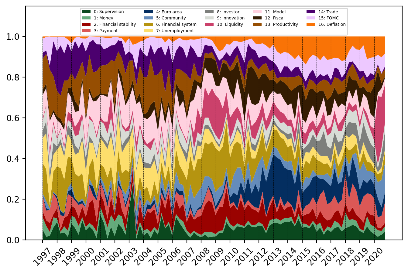
Figure 1: Plot of the average normalized global topic probabilities of the classified documents for each quarter.

Figure 1 shows the average normalized probability distributions for the global topics for each quarter in the sample period, given by the classified documents in the corpus. In each quarter all speeches are classified, their probability distributions averaged (and normalized), and plotted. As seen in the figure, the model captures 17 global topics that are continuously present throughout the sample period, and thus gives an overview of what central banks talk about. The topics are, as expected, primarily about central bank issues, such as monetary policy. However, the analysis shows that the topics are not mainly about coordination of financial market expectations, but addresses a rather broad set of themes. This suggests that central bank communication is not consistent with the traditional view that it is fundamentally used to reveal private information to the public and to affect and coordinate financial market expectations. Figure 1 shows that the central banks’ communication has been seemingly diverse throughout the sample period, targeting a wide range of global topics, including payment systems, small business communities, innovation and technology, economic modelling, and productivity. This holds true also in times were global interest rates have been close to the ELB. One can argue that the topics discussed are in the long run helping the central banks to communicate monetary policy. By informing the public regarding matters such as payment systems or innovation and technology, central banks can build up narratives and prime the economy for future monetary policy paradigm changes. Therefore the communication can be seen as indirectly related to the traditional definition of central bank communication.

Some topics have seemingly constant mass over the sample period, e.g., the topic regarding supervision and regulation. Other topics exhibit clear trends. After the global financial crisis in 2008, one can see a clustering in topics associated with the financial system, financial stability, and liquidity. In contrast, other topics exhibit steady upward trends over time. The topic about the payment system has a positive recent trend, which is in line with contemporary technical advancements in the area. Various countries see clear increases in the amount of digital transactions and many central banks are investigating possibilities for CBDCs.

An advantage of using Dynamic Topic Models, compared to static topic modelling such as LDA, is to be able to follow the topics dynamically through the time dimension. Table 2 shows a sample of the year-by-year evolution of the probability distribution of the topic related to supervision and regulation. The table shows words with the highest probability of being drawn from the topic from years in the beginning and the end of the sample period. One can see that the topic is apparently homogenous over time, indicating that in the beginning of the sample, as well as in the end, the topic is about precisely supervision and regulation. This is important in order to be able to draw more rigid conclusions from further econometric analysis using the estimated topics. If one concludes that there is persistence in a topic it is appropriate to know the content of this topic through time. Furthermore, the dynamic analysis allows for within-topic investigation of the vocabulary distribution. Even though the topic is stable one can see that the vocabulary has changed over time and the probability of other words have increased within the distribution. In Table 2, the token stress test has a higher probability in the end of the sample period. However, the token capital requirement is present as a top word both in 1997 as well as in later years. Note that the persistence in the word-probability distribution of topics is to some extent built into the model. The standard deviation in the model controls the speed at which the topics can evolve on an annually basis. The lower the standard deviation the lower is the variation in topics over time, and with a standard deviation of zero the model becomes static.

1997	1998	1999	…	2018	2019	2020
Supervisor (0.024)	Supervisor (0.024)	Supervisor (0.022)	…	Regulation (0.016)	Regulation (0.016)	Regulation (0.016)
Standard (0.021)	Standard (0.02)	Standard (0.017)	…	Requirement (0.009)	Stress Test (0.01)	Stress Test (0.01)
Approach (0.02)	Approach (0.018)	Approach (0.016)	…	Stress Test (0.009)	Approach (0.009)	Approach (0.01)
Supervisory (0.009)	Supervisory (0.009)	Supervisory (0.008)	…	Approach (0.008)	Requirement (0.009)	Requirement (0.009)
Internal (0.008)	Internal (0.008)	Market Discipline (0.008)	…	Capital Requirement (0.008)	Capital Requirement (0.008)	Rule (0.008)
Institution (0.008)	Institution (0.008)	Institution (0.007)	…	Rule (0.007)	Rule (0.007)	Capital Requirement (0.008)
Risk Management (0.007)	Market Discipline (0.008)	Internal (0.007)	…	Regulatory (0.007)	Regulatory (0.007)	Regulatory (0.008)
Market Discipline (0.007)	Risk Management (0.007)	Risk Management (0.007)	…	Regime (0.006)	Framework (0.007)	Framework (0.007)
Capital Requirement (0.006)	Exposure (0.006)	Exposure (0.007)	…	Standard (0.006)	Regime (0.006)	Regime (0.006)
Exposure (0.006)	Proposal (0.006)	Proposal (0.006)	…	Framework (0.005)	Stress Testing (0.006)	Stress Testing (0.006)

Table 2: Year by year evolution of the probability distribution associated with the topic about supervision and regulation. Sorted probabilities in parenthesis.

Figure 2 shows the probability, throughout the sample, of the tokens; Basel II, Regulation, and Supervisor, from the topic about supervision and regulation. One can see that there has been a shift in language from using the word supervisor to using the word regulation, and the curves intersect around 2008. This is in line with the fact that the global financial crisis led to new regulations in the global financial industry. Furthermore, the token Basel II constitutes a bell shaped curve in Figure 2, with its highest probability just after the Basel II Accord was published in June 2004. The bell shaped pattern matches the theory of epidemiology of narratives discussed in [41]. A narrative starts, it grows, then peaks, and finally declines. Here the underlying narrative is easy to understand, since it depends on the regulations and guidelines issued by the Basel Committee on Banking and Supervision.

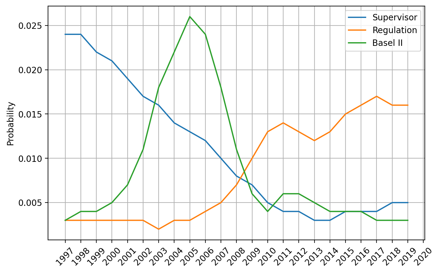
Figure 2: Plot of the average probabilities of the tokens; Basel II, Supervisor, and Regulation, associated with the topic about supervision and regulation.

[21] emphasize the value of human cross-checking when the subsequent results of natural language processing are used beyond prediction, in descriptive or statistical analyses. An auditing of a subsample of twenty to thirty documents will usually give an idea if the model captures the relevant information in the corpus. In topic modelling, it is important to validate that the topics are doing a good job in explaining the documents they are supposedly generating. Documents are generated from a mixture of topics. However, some documents have likely been generated from one topic alone, and are thus excellent candidates for manual investigation. The speech “Implementing Basel II – choices and challenges” by Ms Susan Schmidt Bies at the Fed is the speech in the corpus with the highest probability (99%) of being generated from the topic about supervision and regulation. By reading the speech we can verify this,

In my remarks, I will focus primarily on the choices and challenges associated with Basel II implementation. In particular, I want to reaffirm the Federal Reserve’s commitment to Basel II and the need for continual evolution in risk measurement and management at our largest banks and then discuss a few key aspects of Basel II implementation in the United States. Given the international audience here today, I also plan to offer some thoughts on cross-border implementation issues associated with Basel II, including so-called home-host issues. (Ms Susan Schmidt Bies, Member of the Board of Governors of the US Federal Reserve System, at the Global Association of Risk Professionals’ Basel II and Bakning Regulation Reform, Barcelona, 16 May 2006.)

Overall in this paper, the manual validation (of a small subset) of the speeches suggests that the dimension reduction to topic space captures the content of the documents well.

4.2 Persistence in topics

Next we construct a set of autoregressive (AR) models to investigate the persistence in the estimated global topics. The analyses are based on quarterly data following [3] and [36], as well as monthly data for robustness. The following AR(1) model is estimated for each global topic,

$$\theta_{k,t}=\alpha_{k}+\varphi_{k}\theta_{k,t-1}+\bm{\beta}_{k}\bm{X}_{t}+\bm{\gamma}_{k}\bm{X}_{t-1}+\epsilon_{k,t}.$$ (1)

Here $\theta_{k,t}$ is the average probability for the classified documents at time $t$ for global topic $k$, where $k=1,\dots,K$ and $t=1,\dots,T$. $\bm{X}{t}$ is a vector of region specific control variables at time $t$, used in the Fed case study in Section 5.

Tables LABEL:table:ar_q and LABEL:table:ar_m report the estimated coefficients from the AR(1) model in Equation 1 without regional control variables, using aggregated quarterly and monthly observations for each topic respectively. The tables show strong significant autoregressive effects in the majority of the topics. The results indicate large persistence in the topics, on both quarterly and monthly basis. When central banks talk about a given global topic they tend to continue to do so for some time. An explanation is that the underlying macroeconomic variables that the topics reflect are themselves persistent, which we will control for in the second part of the analysis in Section 5. Another explanation is that narratives drive the persistence in the topics. These narratives can either be part of the global economy or narratives set by the central banks themselves. A few topics are not showing any autoregressive effects. The topic about supervision and regulation does not exhibit any significant persistence, indicating that the topic is talked about sporadically throughout the sample, without specific trends.

5 FED case study

In this section, Equation 1 from Section 4.2 is estimated using the Fed speech data alone, together with regional financial control variables. Central banks tend to address the current economic environment in their communication. Therefore, underlying financial and macroeconomic variables play an important role in determining the topics of central bank communication. Central banks display heterogeneity in the topics addressed, as well as which variables affect their communication. The Fed is more likely to talk about topics related to the US inflation and the US stock market than topics related to European macroeconomic and financial conditions. By selecting speeches from one central bank alone, in this case the Fed, it is possible to control for the regional variables associated with that bank’s speeches.

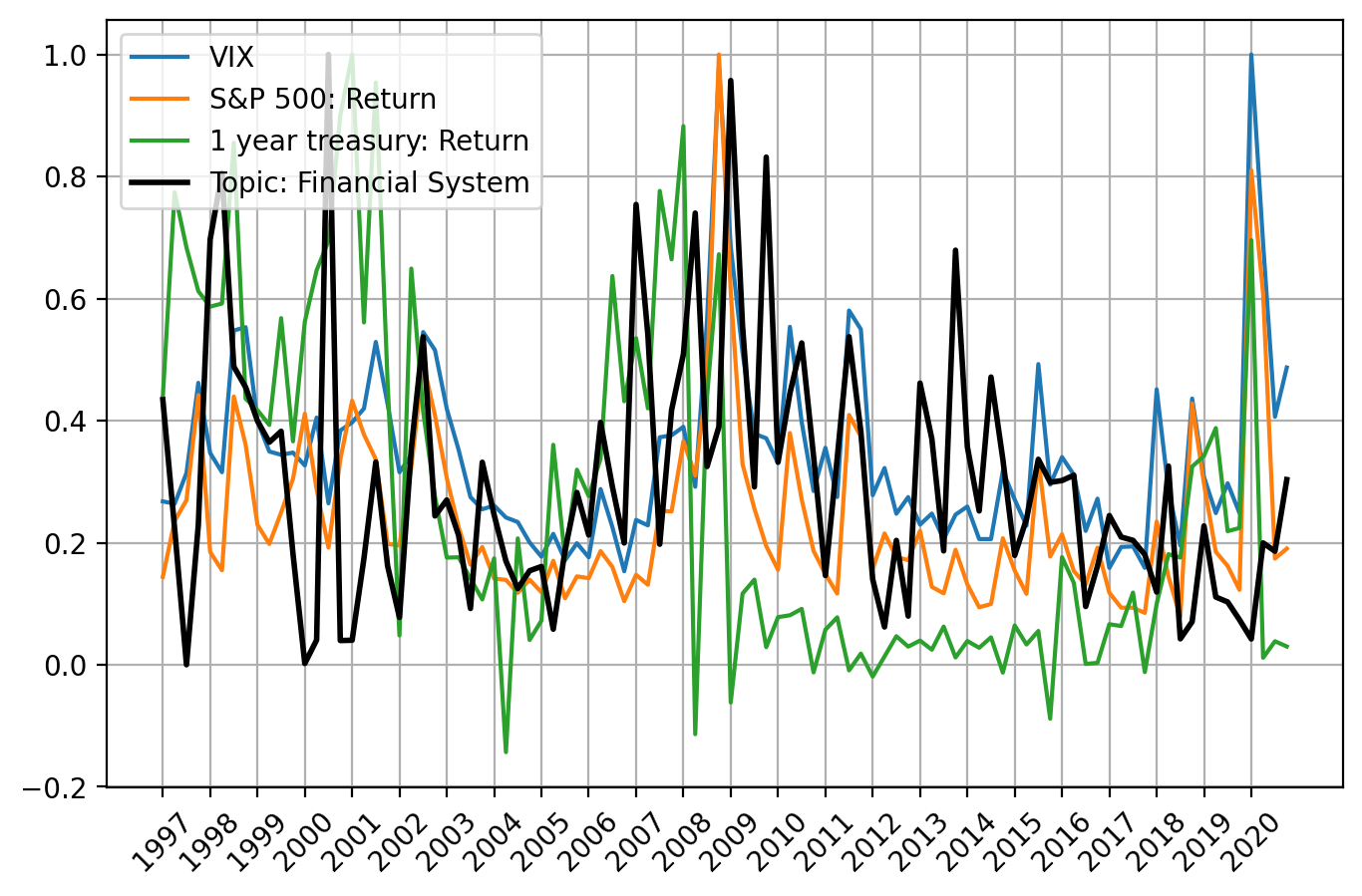
Figure 3: Plot of average quarterly normalized probability of the topic about the financial system, together with three normalized control variables.

Figure 3 illustrates the co-movements between the probability of the topic about the financial system in speeches from the Fed, together with the CBOE Volatility Index (VIX), the S&P 500 Index returns, and 1 year US treasury returns. The figure suggests that there might be a relationship between these variables. Thus, by controlling for the financial variables discussed in the topic about the financial system we might be able to explain the autoregressive feature of the topic. If the persistence is fully explained by the controls, it would suggest that no other effects, such as global narratives or local central bank narratives, are driving the previous observed persistence.

Table LABEL:table:fed_q reports the AR(1) coefficients of the average topic probabilities from 1,841 classified speeches from the Fed and the New York Fed, from 1997 through 2020, without any control variables. Quarterly data are used alone as there are months during the sample period in which no speeches by the Fed were held. The speeches are classified using the DTM model in Section 4. The model is not re-estimated but trained on the full corpus, including speeches from the other 8 central banks analyzed in this paper. Hence, the model is less descriptive of the Fed data, which might be a reason why the results are weaker compared to the previous results in Table LABEL:table:ar_q, Section 4.

The autoregressive properties in the global topics are weakened by adding the controls, but not fully explained, as seen in Table LABEL:table:fed_q_c. Compared to the estimation without the control variables the results show smaller coefficients and lower significance of the persistent topics. But, most topics that exhibit persistence without the controls are also doing so with the controls. Two exceptions are the topic about the financial system and the topic about trade, where the persistence seems to be fully explained by the control variables.

The results from the Fed case study suggest that there are factors other than the underlying financial variables driving the topics’ persistence. Further, the results are consistent with the theory of narrative economics and propose that the communication on topic level is story-based. Story-based communication is more easily spread in conversations, news and social media [41], and coming from a central bank it is more accessible for the general public [23].

6 Conclusion

The empirical findings show that central banks talk about a wide range of global topics, not all immediately related to the traditional theory of central bank communication. The topics are consistent with the literature arguing that the communication is not directly targeting the general public. However, with a broader set of topics, central banks can reveal private information and prepare society for long term monetary policy shifts and structural changes. Topic trends occur and vocabulary changes over time, but most topics have significant probability mass throughout the sample period, even at times when the interest rate is close to the ELB.

Furthermore, the topics are well captured by Dynamic Topic Models. Both in terms of quantitative measures, such as coherence scores, as well as manual investigation linking the topics to the representative documents. Thus, the dimension reduction of the corpus to topic space is able to, in a meaningful way, capture the relevant central bank communication. This encourages the use of topic modelling, and more specifically DTM, in other social science applications with similar data.

Topic modelling has an interesting application in estimating narratives. The observed topic persistence is consistent with the theory of narrative economics and proposes that the central bank communication on topic level is story-based. The evolution of word-probabilities within the topics are also consistent with the epidemiology models of narrative economics.

Appendix A Results

Table 3 shows the full set of estimated topics. Table 4 shows the number of speeches per central bank per year. Table LABEL:table:A_averages shows the average topic distribution for each central bank. The average distributions are calculated by taking the mean over the topic distributions for all classified documents for each central bank. Table 5 shows the full set of coefficients from the Fed caste study in Section 5, including coefficients for the control variables.

Topics	Average $\mathrm{P}$ ($\%$) in corpus
0: Supervision	3.17
1: Money	1.61
2: Financial stability	7.25
3: Payment	2.77
4: Euro area	2.63
5: Community	3.3
6: Financial system	2.56
7: Unemployment	1.61
8: Investor	5.33
9: Innovation	2.63
10: Liquidity	1.93
11: Model	4.37
12: Fiscal	5.51
13: Productivity	3.88
14: Trade	4.37
15: FOMC	2.14
16: Deflation	2.55
Sum global:	57.61
17: Australia	2.97
18: Canada	7.02
19: ECB	3.01
20: Euro area	4.54
21: Federal reserve	4.67
22: Japan economy	1.76
23: Japan	5.29
24: Norway	2.12
25: Riksbank	2.89
26: Residual	4.08
27: SNB	2.54
28: UK	1.53
Sum local:	42.39
Mean	3.45
Sum	100.0

Table 3: Estimated topics, both local and global, and respectively probabilities in corpus.

	1997	1998	1999	2000	2001	2002	2003	2004	2005	2006	2007	2008	2009	2010	2011	2012	2013	2014	2015	2016	2017	2018	2019	2020	Sum
CAN	7	6	9	9	12	18	18	18	24	25	29	24	24	23	31	25	28	22	23	27	26	29	19	23	499
ENG	13	15	12	22	21	14	7	10	12	17	17	21	28	38	34	25	36	37	47	38	37	44	48	32	625
JPN	21	16	15	22	16	21	28	15	20	14	19	18	32	32	45	50	42	44	35	33	39	27	40	24	668
FED	52	43	42	39	48	55	55	97	86	76	85	88	70	73	62	51	59	46	57	42	54	49	79	57	1465
NOR	0	0	6	7	10	19	14	13	20	20	15	16	17	16	11	10	10	8	8	8	10	9	10	5	262
ECB	0	8	46	45	36	40	31	56	51	58	88	149	130	121	139	103	152	130	136	120	169	135	143	99	2185
NYC	5	7	5	7	2	4	3	8	10	12	9	4	11	23	22	18	29	26	34	32	29	26	28	22	376
AUS	9	12	9	12	8	12	11	9	13	9	10	17	17	29	32	27	26	26	34	25	33	38	34	23	475
SWE	11	13	28	31	29	29	21	24	23	36	22	27	23	25	28	15	17	13	9	11	5	12	8	6	466
CHE	1	1	3	2	4	11	11	28	27	27	26	29	25	19	16	21	15	14	16	15	10	16	14	7	358
Sum	119	121	175	196	186	223	199	278	286	294	320	393	377	399	420	345	414	366	399	351	412	385	423	298	7379

Table 4: Number of speeches per central bank per year.

	(1)	(2)	(3)	(4)	(5)	(6)	(7)	(8)	(9)	(10)	(11)	(12)	(13)	(14)	(15)	(16)	(17)
	Regu- lation	Money	Financial stability	Payment	Euro area	Comm- unity	Financial system	Unemp- loyment	Investor	Inno- vation	Liqui- dity	Model	Fiscal	Produ- ctivity	Trade	FOMC	Deflation
1 Lag	0.0211	0.170	0.174	0.381∗∗	0.583∗∗∗	0.309	0.262	0.270∗	0.367∗∗∗	0.0928	0.542∗∗∗	-0.0121	0.334∗	0.421∗∗∗	0.127	0.114	0.479∗∗∗
	(0.18)	(1.37)	(1.60)	(2.81)	(5.48)	(1.93)	(1.88)	(2.15)	(3.79)	(0.79)	(4.51)	(-0.10)	(2.25)	(4.06)	(0.98)	(1.31)	(3.94)
Inflation	-0.217	0.0326	-0.0803	-0.396	-0.305	-0.141	0.225	-0.145	-0.108	0.0291	-0.416	0.373	0.518	0.645	0.165	0.383	0.114
	(-0.57)	(0.24)	(-0.13)	(-1.21)	(-1.08)	(-0.39)	(0.53)	(-0.46)	(-0.71)	(0.13)	(-1.20)	(1.31)	(1.15)	(1.41)	(0.44)	(1.37)	(0.35)
Lag Inflation	-0.165	-0.366∗∗	-0.125	0.375	0.0950	-0.0224	-0.381	0.350	-0.157	0.204	-0.0432	0.212	0.0725	-0.175	-0.0773	-0.586	-0.525
	(-0.49)	(-3.33)	(-0.30)	(1.09)	(0.24)	(-0.06)	(-0.84)	(1.32)	(-0.88)	(0.76)	(-0.11)	(0.69)	(0.17)	(-0.42)	(-0.26)	(-1.56)	(-1.84)
1 year bond	-0.793	-0.0410	-0.778	-0.251	-0.301	-0.925	-0.596	1.587∗∗	0.237	-0.223	-1.578∗	-0.384	-0.684	-0.0599	2.037∗∗	-0.259	0.0466
	(-1.66)	(-0.14)	(-1.10)	(-0.39)	(-0.63)	(-1.59)	(-0.70)	(2.90)	(0.84)	(-0.49)	(-2.16)	(-0.70)	(-1.24)	(-0.06)	(3.12)	(-0.42)	(0.11)
Lag 1 year bond	-0.00155	0.142	-0.323	0.493	-1.148∗	-0.0752	1.010	-0.161	-0.388	0.384	0.943	0.549	-0.953	0.611	0.151	-0.336	-1.151∗
	(-0.00)	(0.41)	(-0.45)	(0.69)	(-2.15)	(-0.11)	(1.30)	(-0.28)	(-1.44)	(0.86)	(1.32)	(1.17)	(-1.37)	(0.82)	(0.25)	(-0.57)	(-2.33)
SP500 returns	-0.244	-0.394∗	1.201∗	-0.275	0.424	0.0697	-0.299	0.0832	-0.635∗	0.166	0.313	1.319∗∗	-0.0479	0.773	-0.0949	0.158	-0.213
	(-0.47)	(-2.04)	(1.99)	(-0.47)	(1.13)	(0.11)	(-0.48)	(0.19)	(-2.49)	(0.50)	(0.63)	(2.93)	(-0.10)	(1.35)	(-0.22)	(0.38)	(-0.59)
Lag SP500 returns	0.331	-0.184	-0.176	-0.0587	0.258	-0.00507	0.157	-0.0580	0.273	0.450	-0.0878	-0.685	-0.327	-0.223	-0.258	-0.159	0.186
	(0.73)	(-0.92)	(-0.37)	(-0.11)	(0.50)	(-0.01)	(0.27)	(-0.18)	(1.01)	(0.91)	(-0.17)	(-1.53)	(-0.70)	(-0.41)	(-0.62)	(-0.33)	(0.46)
VIX	0.0000797	0.000707∗	-0.000968	0.000413	-0.000873	0.000115	0.000524	-0.000402	0.000834∗	-0.000293	0.000172	-0.00175∗∗	0.000750	-0.000922	-0.000430	-0.000179	0.000363
	(0.13)	(2.40)	(-1.40)	(0.54)	(-1.57)	(0.14)	(0.68)	(-0.73)	(2.03)	(-0.64)	(0.28)	(-2.97)	(1.11)	(-1.15)	(-0.68)	(-0.30)	(0.47)
Lag VIX	-0.000614	-0.000143	0.000469	-0.000207	-0.000109	0.000461	0.0000854	0.000188	-0.000656	-0.000881	0.000762	0.000661	0.0000888	-0.000413	0.000365	-0.000162	-0.000240
	(-1.00)	(-0.47)	(0.52)	(-0.27)	(-0.14)	(0.66)	(0.10)	(0.39)	(-1.94)	(-1.24)	(0.82)	(0.95)	(0.15)	(-0.56)	(0.59)	(-0.21)	(-0.46)
Constants	0.0497∗∗∗	0.0112∗∗	0.0258	0.0191∗	0.0332∗	0.0122	0.0208	0.0192∗∗	0.0201∗	0.0401∗∗∗	-0.0118	0.0572∗∗∗	0.0183	0.0405∗∗	0.0310∗∗	0.0472∗∗∗	0.0206
	(4.49)	(2.77)	(1.58)	(2.01)	(2.35)	(0.83)	(1.82)	(2.85)	(2.46)	(3.95)	(-0.74)	(4.37)	(1.43)	(3.36)	(3.03)	(3.60)	(1.84)
$N$	95	95	95	95	95	95	95	95	95	95	95	95	95	95	95	95	95
t statistics in parentheses
∗ $p<0.05$, ∗∗ $p<0.01$, ∗∗∗ $p<0.001$

Table 5: Estimated coefficients from the AR(1) models with control variables, using quarterly data from the Fed. Each equation is represented as a column. The t-statistics (reported in parenthesis) are based on [34] standard errors with 1 lag.

Appendix B Fed robustness

Figure 4 shows the average normalized probability distributions for the topics for each quarter, given by the classified documents using DTM trained on the data from the Fed and the New York Fed alone. In each quarter all speeches are classified, their probability distributions averaged, and plotted.

Compared to the main model in the paper, one can see that the topic about supervision and regulation has split into two topics. The patterns of the topics are familiar, and here expressed by a higher probability of the topic related to supervision in the beginning of the corpus, and a higher probability of the topic related to regulation in the end.

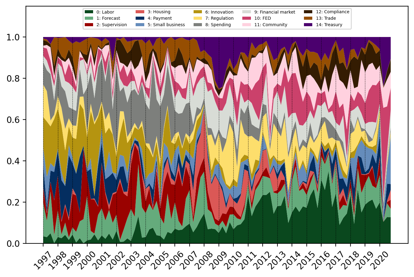
Figure 4: Plot of the average probabilities of topics over each quarter.

Table 6 reports the estimated coefficients of the AR(1) models estimated using data from a topic model trained on data from the Fed and the New York Fed alone.

	(1)	(2)	(3)	(4)	(5)	(6)	(7)	(8)	(9)	(10)	(11)	(12)	(13)	(14)	(15)
	Labor	Forecast	Supervision	Housing	Payment	Small business	Innovation	Regulation	Spending	Financial markets	FED	Community	Compliance	Trade	Treasury
1 Lag	0.672∗∗∗	0.171	0.241	0.797∗∗∗	0.0876	0.132	0.640∗∗∗	0.489∗∗∗	0.464∗∗∗	0.402∗∗∗	0.579∗∗∗	0.277∗	0.567∗∗∗	0.226∗	0.519∗∗∗
	(7.68)	(1.60)	(1.87)	(7.95)	(0.70)	(1.13)	(6.63)	(4.26)	(3.91)	(3.71)	(5.49)	(2.31)	(5.90)	(2.55)	(5.15)
Inflation	0.882	1.024∗	-0.115	-0.588	-0.224	0.0300	0.398	-0.266	0.946	-0.134	-0.707	0.468	-0.107	-0.141	-1.342∗∗
	(1.54)	(2.03)	(-0.15)	(-1.00)	(-0.45)	(0.08)	(0.67)	(-0.52)	(1.14)	(-0.23)	(-1.35)	(1.00)	(-0.28)	(-0.31)	(-2.90)
Lag Inflation	-1.284∗	-1.517∗∗	1.844∗	-0.609	0.0924	-0.342	0.872∗	-0.0738	-0.545	1.087	0.298	0.753	-0.0731	-0.104	-0.292
	(-2.45)	(-2.85)	(2.16)	(-1.61)	(0.25)	(-0.72)	(2.28)	(-0.10)	(-0.57)	(1.68)	(0.35)	(1.54)	(-0.17)	(-0.27)	(-0.71)
1 year bond	0.404	0.915	1.204	1.032	2.253	1.403	1.162	0.288	2.605	-1.660	-3.243∗	-2.436∗∗∗	-0.0541	-0.0578	-1.456
	(0.45)	(0.89)	(0.72)	(1.38)	(1.76)	(1.51)	(0.88)	(0.33)	(1.24)	(-1.80)	(-2.08)	(-3.69)	(-0.08)	(-0.09)	(-1.84)
Lag 1 year bond	-2.348∗∗	0.341	2.363	-0.295	2.467	-1.662	1.556	-2.346∗	-0.589	0.891	1.720	-0.474	-0.527	1.327	-0.119
	(-2.87)	(0.38)	(1.32)	(-0.51)	(1.79)	(-1.98)	(1.51)	(-2.04)	(-0.21)	(0.91)	(1.33)	(-0.55)	(-0.84)	(1.90)	(-0.14)
SP500 returns	-1.454∗	0.569	0.862	0.330	-2.589∗∗	-0.235	-0.246	-0.794	0.0402	0.303	1.481	0.693	0.182	-0.0307	0.499
	(-2.34)	(0.61)	(0.76)	(0.55)	(-2.88)	(-0.27)	(-0.36)	(-1.10)	(0.04)	(0.49)	(1.25)	(0.99)	(0.39)	(-0.06)	(0.77)
Lag SP500 returns	0.112	0.135	-0.125	-0.338	0.284	-0.141	0.210	0.779	0.130	-0.410	-0.438	-0.188	-0.337	-0.312	0.395
	(0.15)	(0.17)	(-0.12)	(-0.60)	(0.31)	(-0.18)	(0.27)	(0.92)	(0.08)	(-0.73)	(-0.46)	(-0.30)	(-0.61)	(-0.54)	(0.59)
VIX	0.00232∗	-0.00102	-0.00154	-0.000343	0.00362∗∗	0.000210	-0.000281	0.000446	-0.000613	0.000131	-0.00170	-0.000469	-0.000563	-0.000418	-0.000140
	(2.57)	(-0.82)	(-0.97)	(-0.43)	(3.04)	(0.15)	(-0.31)	(0.45)	(-0.40)	(0.17)	(-1.28)	(-0.52)	(-0.80)	(-0.62)	(-0.18)
Lag VIX	-0.000877	-0.00135	0.000293	0.000483	-0.000948	0.000859	-0.000203	-0.000150	-0.000193	0.000230	0.00127	-0.000238	0.000594	-0.000314	0.000576
	(-0.70)	(-1.20)	(0.18)	(0.55)	(-0.74)	(0.75)	(-0.18)	(-0.12)	(-0.10)	(0.26)	(0.67)	(-0.27)	(0.60)	(-0.39)	(0.56)
Constants	0.0481	0.114∗∗∗	0.0385	0.00583	0.00329	0.0230	0.0153	0.0410∗	0.0528∗	0.0373∗	0.0263	0.0689∗∗	0.0277	0.0594∗∗∗	0.00835
	(1.97)	(5.30)	(1.57)	(0.48)	(0.18)	(1.24)	(1.06)	(2.44)	(2.24)	(2.08)	(0.86)	(3.30)	(1.86)	(4.00)	(0.53)
$N$	95	95	95	95	95	95	95	95	95	95	95	95	95	95	95
t statistics in parentheses
∗ $p<0.05$, ∗∗ $p<0.01$, ∗∗∗ $p<0.001$

Table 6: Estimated coefficients from the AR(1) models, using quarterly data from the Fed. The documents are classified with a DTM model trained on the Fed speeches alone. Each equation is represented as a column. The t-statistics (reported in parenthesis) are based on [34] standard errors with 1 lag.

References

- [1] Jeffery D. Amato, Stephen Morris and Hyun Song Shin “Communication and Monetary Policy” In Oxford Review of Economic Policy 18.4, 2002, pp. 495–503 DOI: 10.1093/oxrep/18.4.495
- [2] Malin Andersson, Hans Dillén and Peter Sellin “Monetary policy signaling and movements in the term structure of interest rates” In Journal of Monetary Economics 53.8, 2006, pp. 1815–1855 DOI: https://doi.org/10.1016/j.jmoneco.2006.06.002
- [3] Hanna Armelius, Christoph Bertsch, Isaiah Hull and Xin Zhang “Spread the Word: International spillovers from central bank communication” In Journal of International Money and Finance 103, 2020, pp. 102116 DOI: https://doi.org/10.1016/j.jimonfin.2019.102116
- [4] Bank for International Settlements “Central bank digital currencies: foundational principles and core features”, 2020
- [5] Roland Barthes and Lionel Duisit “An Introduction to the Structural Analysis of Narrative” In New Literary History 6.2 Johns Hopkins University Press, 1975, pp. 237–272 URL: http://www.jstor.org/stable/468419
- [6] Steven Bird, Edward Loper and Klein Ewan “Natural Language Processing with Python” O’Reilly Media Inc., 2009
- [7] David Blei and John Lafferty “Dynamic Topic Models” In Proceedings of the 23rd International Conference on Machine Learning, ICML ’06 Pittsburgh, Pennsylvania, USA: Association for Computing Machinery, 2006, pp. 113–120 DOI: 10.1145/1143844.1143859
- [8] David Blei and John Lafferty “A correlated topic model of Science” In The Annals of Applied Statistics 1, 2007 DOI: 10.1214/07-AOAS114
- [9] David Blei, Andrew Ng and Michael Jordan “Latent Dirichlet Allocation” In The Journal of Machine Learning Research 3, 2003, pp. 993–1022
- [10] Alan S. Blinder “Through a Crystal Ball Darkly: The Future of Monetary Policy Communication” In AEA Papers and Proceedings 108 American Economic Association, 2018, pp. 567–571 URL: https://www.jstor.org/stable/26452803
- [11] Alan S. Blinder, Michael Ehrmann, Marcel Fratzscher, Jakob Haan and David-Jan Jansen “Central Bank Communication and Monetary Policy: A Survey of Theory and Evidence” In Journal of Economic Literature 46.4 American Economic Association, 2008, pp. 910–945 URL: http://www.jstor.org/stable/27647085
- [12] Benjamin Born, Michael Ehrmann and Marcel Fratzscher “Central Bank Communication on Financial Stability” In The Economic Journal 124.577 Wiley, 2014, pp. 701–734 URL: http://www.jstor.org/stable/42919216
- [13] William C. Brainard “Uncertainty and the Effectiveness of Policy” In The American Economic Review 57.2 American Economic Association, 1967, pp. 411–425 URL: http://www.jstor.org/stable/1821642
- [14] Jerome Bruner “The Narrative Construction of Reality” In Critical Inquiry 18.1 The University of Chicago Press, 1991, pp. 1–21 URL: http://www.jstor.org/stable/1343711
- [15] John H. Cochrane and Monika Piazzesi “The Fed and Interest Rates: A High-Frequency Identification” In The American Economic Review 92.2 American Economic Association, 2002, pp. 90–95 URL: http://www.jstor.org/stable/3083383
- [16] Olivier Coibion, Yuriy Gorodnichenko, Saten Kumar and Mathieu Pedemonte “Inflation expectations as a policy tool?” NBER International Seminar on Macroeconomics 2019 In Journal of International Economics 124, 2020, pp. 103297 DOI: https://doi.org/10.1016/j.jinteco.2020.103297
- [17] Timothy Cook and Thomas Hahn “The effect of changes in the federal funds rate target on market interest rates in the 1970s” In Journal of Monetary Economics 24.3, 1989, pp. 331–351 DOI: https://doi.org/10.1016/0304-3932(89)90025-1
- [18] Scott Deerwester, Susan T. Dumais, George W. Furnas, Thomas K. Landauer and Richard Harshman “Indexing by Latent Semantic Analysis” Copyright - Copyright Wiley Periodicals Inc. Sep 1990; Last updated - 2019-11-23; SubjectsTermNotLitGenreText - New York In Journal of the American Society for Information Science (1986-1998) 41.6, 1990, pp. 391 URL: https://search-proquest-com.ezproxy.ub.gu.se/docview/216891549?accountid=11162
- [19] Saskia Ellen, Vegard H. Larsen and Leif Anders Thorsrud “Narrative monetary policy surprises and the media”, 2019 URL: https://ideas.repec.org/p/bny/wpaper/0078.html
- [20] European Commission “Standard Eurobarometer (EB 92) – Public opinions in the European Union”, 2019
- [21] Matthew Gentzkow, Bryan Kelly and Matt Taddy “Text as Data” In Journal of Economic Literature 57.3 American Economic Association, 2019, pp. 535–574
- [22] Thomas L. Griffiths and Mark Steyvers “Finding scientific topics” In Proceedings of the National Academy of Sciences 101.suppl 1 National Academy of Sciences, 2004, pp. 5228–5235 DOI: 10.1073/pnas.0307752101
- [23] Andrew Haldane and Michael McMahon “Central Bank Communications and the General Public” In AEA Papers and Proceedings 108, 2018, pp. 578–83 DOI: 10.1257/pandp.20181082
- [24] Stephen Hansen, Michael McMahon and Andrea Prat “Transparency and Deliberation Within the FOMC: A Computational Linguistics Approach*” In The Quarterly Journal of Economics 133.2, 2017, pp. 801–870 DOI: 10.1093/qje/qjx045
- [25] Stephen Hansen, Michael McMahon and Matthew Tong “The long-run information effect of central bank communication” “Central Bank Communications:From Mystery to Transparency”May 23-24, 2019Annual Research Conference ofthe National Bank of UkraineOrganized in cooperation withNarodowy Bank Polski In Journal of Monetary Economics 108, 2019, pp. 185–202 DOI: https://doi.org/10.1016/j.jmoneco.2019.09.002
- [26] Bernd Hayo and Edith Neuenkirch “The German public and its trust in the ECB: The role of knowledge and information search” In Journal of International Money and Finance 47, 2014, pp. 286–303 DOI: https://doi.org/10.1016/j.jimonfin.2014.07.003
- [27] Thomas Hofmann “Probabilistic latent semantic indexing” In SIGIR ’99, 1999
- [28] David-Jan Jansen and Jakob De Haan “Talking heads: the effects of ECB statements on the euro–dollar exchange rate” Exchange Rate Economics In Journal of International Money and Finance 24.2, 2005, pp. 343–361 DOI: https://doi.org/10.1016/j.jimonfin.2004.12.009
- [29] Saten Kumar, Olivier Coibion, Hassan Afrouzi and Yuriy Gorodnichenko “Inflation Targeting Does Not Anchor Inflation Expectations: Evidence from Firms in New Zealand” In Brookings Papers on Economic Activity Brookings Institution Press, 2015, pp. 151–208 URL: http://www.jstor.org/stable/43752171
- [30] Michael J. Lamla and Dmitri V. Vinogradov “Central bank announcements: Big news for little people?” “Central Bank Communications:From Mystery to Transparency”May 23-24, 2019Annual Research Conference ofthe National Bank of UkraineOrganized in cooperation withNarodowy Bank Polski In Journal of Monetary Economics 108, 2019, pp. 21–38 DOI: https://doi.org/10.1016/j.jmoneco.2019.08.014
- [31] Andrew Kachites McCallum “MALLET: A Machine Learning for Language Toolkit” http://mallet.cs.umass.edu, 2002
- [32] W… Mitchell “On narrative” In On narrative, Phoenix book Chicago ;: University of Chicago Press, 1981
- [33] Emi Nakamura and Jón Steinsson “High-Frequency Identification of Monetary Non-Neutrality: The Information Effect*” In The Quarterly Journal of Economics 133.3, 2018, pp. 1283–1330 DOI: 10.1093/qje/qjy004
- [34] Whitney K. Newey and Kenneth D. West “A simple, positive semi-definite, heteroskedasticity and autocorrelation consistent covariance matrix” In Econometrica 55 Blackwell Publishers Ltd., 1987, pp. 703
- [35] David Newman, Jey Lau, Karl Grieser and Timothy Baldwin “Automatic Evaluation of Topic Coherence.” In Human Language Technologies: The 2010 Annual Conference of the North American Chapter of the ACL, 2010, pp. 100–108
- [36] Rickard Nyman, Sujit Kapadia, David Tuckett, David Gregory, Paul Ormerod and Robert Smith “News and Narratives in Financial Systems: Exploiting Big Data for Systemic Risk Assessment” In SSRN Electronic Journal, 2018 DOI: 10.2139/ssrn.3135262
- [37] Christos H. Papadimitriou, Prabhakar Raghavan, Hisao Tamaki and Santosh Vempala “Latent Semantic Indexing: A Probabilistic Analysis”, 1997
- [38] Radim Řehůřek and Petr Sojka “Software Framework for Topic Modelling with Large Corpora” http://is.muni.cz/publication/884893/en In Proceedings of the LREC 2010 Workshop on New Challenges for NLP Frameworks Valletta, Malta: ELRA, 2010, pp. 45–50
- [39] Michael Röder, Andreas Both and Alexander Hinneburg “Exploring the Space of Topic Coherence Measures” In Proceedings of the Eighth ACM International Conference on Web Search and Data Mining, WSDM ’15 Shanghai, China: Association for Computing Machinery, 2015, pp. 399–408 DOI: 10.1145/2684822.2685324
- [40] Theodore R Sarbin “Narrative psychology: The storied nature of human conduct.” Praeger Publishers/Greenwood Publishing Group, 1986
- [41] Robert J. Shiller “Narrative Economics” In American Economic Review 107.4, 2017, pp. 967–1004 DOI: 10.1257/aer.107.4.967
- [42] Yee Whye Teh, Michael I. Jordan, Matthew J. Beal and David M. Blei “Sharing Clusters among Related Groups: Hierarchical Dirichlet Processes” In Proceedings of the 17th International Conference on Neural Information Processing Systems, NIPS’04 Vancouver, British Columbia, Canada: MIT Press, 2004, pp. 1385–1392
- [43] Hanna M. Wallach, Iain Murray, Ruslan Salakhutdinov and David Mimno “Evaluation Methods for Topic Models” In Proceedings of the 26th Annual International Conference on Machine Learning, ICML ’09 Montreal, Quebec, Canada: Association for Computing Machinery, 2009, pp. 1105–1112 DOI: 10.1145/1553374.1553515
- [44] Michael Woodford “Monetary policy in the information economy” In Proceedings - Economic Policy Symposium - Jackson Hole, 2001, pp. 297–370 URL: https://ideas.repec.org/a/fip/fedkpr/y2001p297-370.html
- [45] Michael Woodford “Central Bank Communication and Policy Effectiveness”, Working Paper Series 11898, 2005 DOI: 10.3386/w11898