Search For Deep Graph Neural Networks

Abstract

Current GNN oriented NAS methods focus on the search for different layer aggregate components with shallow and simple architectures, which are limited by the “over-smooth” problem.

To further explore the benefits from structural diversity and depth of GNN architectures, we propose a GNN generation pipeline with a novel two-stage search space, which aims at automatically generating high-performance while transferable deep GNN models in a block-wise manner. Meanwhile, to alleviate the “over-smooth” problem, we incorporate multiple flexible residual connection in our search space and apply identity mapping in the basic GNN layers. For the search algorithm, we use deep-q-learning with epsilon-greedy exploration strategy and reward reshaping. Extensive experiments on real-world datasets show that our generated GNN models outperforms existing manually designed and NAS-based ones.

1 Introduction

Graph Neural Networks (GNNs), a class of deep learning models designed for performing information interaction on non-Euclidean graph data, have been successfully applied to applications of various domains such as recommender systems [44, 25], physics [3, 32, 34] and natural language processing [45, 12, 20]. Although GNNs and their variants [9, 14, 40, 41] have shown convincing performance in a variety of graph datasets, the design of graph convolutional layers often require domain knowledge and laborious human involvement. Moreover, unlike most CNN models in computer vision tasks, GNNs often show poor transferability toward different scenarios, and require additional manual adjustments when dealing with new tasks.

Meanwhile, emerged as a powerful tool for automatic neural network optimization, neural network architecture search (NAS) [50, 29, 26, 19, 18] has been widely applied for discovering high-performance network architectures in convolutional neural networks (CNNs) and recurrent neural networks (RNNs). Recently, GraphNAS [7] has made the first attempt to apply NAS method to graph data by utilizing existing GNN layers to build the final architecture while leveraging the power of RNN with policy gradient to adaptively optimize the model, followed by several related works as Auto-GNN [49] and SNAG [46].

However, both the hand-crafted and NAS-designed GNN models are constrained by “over-smooth” problem [5] thus share a simple and shallow architecture. For example, GCN [14], GAT [40] and GraphNAS [7] only stack 2 layers for the transductive learning tasks, while SNAG chooses 3 layers. Although achieving their best performance, such a shallow structure limits the model’s ability to extract information from high-order neighbors, and the potential power brought by structure diversity is underutilized. Some recent works have made efforts to explore different GNN structures, such as Inception-like module [31], DenseNet-like snowball structure [22], as well as deeper GNN models [6, 16]. Although these works show possible benefits brought by GNN structural diversity and depth, the structurally diversified GNN design space is not fully explored.

In this work, we aim at digging deeper into the potential benefits of GNN architectures’ diversity and depth, and propose a novel GNN generation pipeline to automatically search for high-performance GNN models. As is mentioned in [7], GNN architecture search suffers from an exponentially growing search space, especially when the layer number increases. To cope with such problem, we propose a two-stage search space that incorporates various flexible model structures such as inception-like module and residual connection, while also greatly reduces the number of candidate models when the overall depth grows. Besides, to further alleviate the “over-smooth” problem in deep GNN layers, we apply initial residual connection [15] and identity mapping [6] to our basic graph convolutional layers. Finally, our search space still contains billions of possible GNN architectures even after pruning. To effectively explore our proposed search space, we apply the deep-q-learning algorithm (DQN) [23] with epsilon-greedy strategy, accompanied with reward reshaping technique [27] and experience replay [17] that further accelerate and stabilize the search process.

Highlights of our work are listed as follows:

1. Deep and flexible GNN architecture: We extend the initial residual connection and identity mapping to various GNN layers thus achieve deep and high-performance GNN models. To fully exploit structural diversity, we also incorporate flexible GNN stacking rules in our search space, which could emulate efficient structures such as residual and inception-like modules.

2. Two-stage search space: We propose a block-wise GNN architecture generation pipeline, and divide the overall search space into two stages, as block-wise and architecture-wise search, which greatly reduces the exponentially growing search space and improves search efficiency.

3. Transfererble GNN blocks: Unlike most current GNN structure, our generated GNN block in the first-stage space could be easily transferred to other datasets without researching, while retaining high accuracy.

2 Related Work

2.1 Neural Network Architecture Search

Reinforcement Learning based neural network architecture search (NAS) was initially proposed by [50] and [2], and yield better performance compared with traditional evolutionary based NAS methods [33, 37, 36, 38]. However, directly searching for the overall architecture of CNNs and RNNs is computationally expensive, especially in big dataset, as the search space grows exponentially when the scale of architecture increases. Based on this, [47] proposed to break the CNN architectures into blocks, and search the structure of a single block only. The generated block was then used to construct the final architecture. In this work, we propose to apply block-wise search in our first-stage search space, which consists multiple different GNN layers connected with each other in a residual or inception-like manner. Then we use the second-stage search space to control the overall model depth and macro residual connections.

2.2 Graph Neural Network Architecture

Designed for learning in graph domains, Graph Neural Networks (GNNs) are initially proposed in [8], with promising performance presented in recent GNN variants [40, 14, 9]. Generally, GNNs could learn node embeddings by performing graph convolutions among adjacent notes, which can be formulated as:

$$x_{i}^{(l+1)}=\delta(x_{i}^{(l)},\ \sigma_{j\in\theta(\mathcal{N}(i))}\gamma(x_{i}^{(l)},x_{j}^{(l)}))$$ (1)

Then, inspired by the success of applying NAS technique in CNN and RNN model optimization, several works have attempted to automatically search for good GNN architectures using existing graph convolutional layers [49, 7, 46]. However, these NAS generated GNN models share simple and shallow structures, which underutilizes the information from high-order neighbors. In this work, we propose to search for deep while flexible GNN architecture by incorporating residual and inception-like module in our search space. To cope with the growing search space problem in [7], we use transferable GNN blocks to construct the final architecture. We also apply initial residual connection [15] and identity mapping [6] to further alleviate the “over-smooth” problem. In experiments, our model consisting of 30 layers reaches the best performance, and both our block and final architecture show great transferability toward different tasks and datasets.

3 Methodology

In this section, we first define our problem and search objective. Then we present a general representation of GNN layers with identity mapping and initial residual connection, in order to extend these two technique to various graph convolutional layers. After this, we introduce our proposed two-stage search space with corresponding basic components. Finally, we elaborate our deep-q-learning agent equipped with experience replay and reward reshaping, and illustrate the search process in each stage.

3.1 Problem Formulation

The overall search object of this work could be formulated as:

$$M^{*}=argmax_{M\in{S}}\ \mathbb{E}[R_{V}(M)]$$ (2)

where $S$ is the overall two-stage search space consists of $S_{B}$ and $S_{A}$ denoting block-wise and architecture-wise search space respectively. $R_{V}(M)$ denotes the model’s evaluated accuracy (reward) on the validation set $V$. The aim of this work is to find the best GNN model $M^{*}\in S$ that achieves highest expected accuracy $\mathbb{E}[R_{V}(M^{*})]$.

Meanwhile, as our model generation is a progressive process among the two-stage search space, we can not directly excavate the best model $M^{*}$ in $S$. Thus, we further define the sub-goal of architecture search in each stage as:

$$B^{*}=argmax_{B\in{S_{B}}}\ \mathbb{E}[R_{V}(M^{\prime}_{B})]$$ (3)

$$A^{*}=argmax_{A\in{S_{A}}}\ \mathbb{E}[R_{V}(M_{A})]$$ (4)

where $B$ and $A$ denote for GNN block and architecture respectively, while each $B$ is composed by basic GNN layers and $A$ could contain multiple kinds of generated high-performance GNN blocks. Note that $M^{\prime}_{B}$ is the standard model constructed by block $B$, as depicted in Figure 2(b) , with similar architecture depth defined in the second search space. And $M_{A}$ is the GNN model directly decided by architecture $A$.

3.2 Identity Mapping & Initial Residual Connect

While searching for deep GNN architecture, our model could severely suffer from the “over-smooth” problem [48]. Recently, APPNP [15] applied initial residual connection in the context of Personalized PageRank to alleviate this problem, but failed to achieve a deep model. Following [15], GCNII [6] further pointed out that solely applying initial residual connection is not sufficient. Inspired by Resnet [10], they utilized identity mapping as supplement for initial residual connection, which successfully deepened GCN model to 64 layers and achieved top performance. Inspired by these works, we propose to extend these two techniques to other graph convolutional layers, and then utilize these layers as basic components of our GNN blocks. Here, we present a general representation of a GNN layer with identity mapping and initial residual connection as:

$$h_{i}^{l+1}=\sigma_{j\in\mathcal{N}(i)}[((1-\alpha)c_{ij}h_{j}+\alpha h^{(0)}_{j})((1-\beta)+\beta\theta_{ij})]$$ (5)

where $h_{i}^{(l)}$ is the embedding for node $i$ in layer $l$. $\alpha$ and $\beta$ are two hyper-parameters that control the weight for residual connection from the initial embedding $h_{j}^{(0)}$ and identity mapping for the weight matrix $\theta_{ij}$ respectively. And $c_{ij}$ denotes the coefficients between target node $i$ and its one-hop adjacent node $j$. For example, $c_{ij}$ is the attention coefficients $a_{ij}$ in GAT [40] and $\frac{1}{\sqrt{d_{i}d_{j}}}$ in GCN [14]. Finally, a permutation invariant aggregation function $\sigma$ is applied to aggregate features from adjacent nodes.

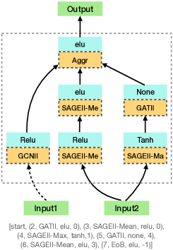
(a) GNN block

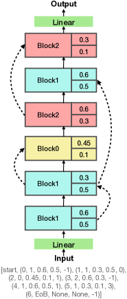
(b) GNN architecture

Figure 1: Left: Illustration of a block with corresponding representative block code. Each layer in the block is depicted as a 4-D vector. e.g. (2, GATII, elu, 0). Right: Schematic depiction of a GNN architecture constructed by three types of blocks, with corresponding architecture code. Each block is depicted as a 5-D vector. Note that dashed lines with arrows denote for residual connections.

3.3 Two-stage Search Space

In this section, we elaborate our proposed search space for graph neural network generation. Inspired by the design of modern CNNs, e.g. Resnet [10] and Inception [39], that stack multiple hand-crafted CNN blocks to construct the final architecture, we divide the search process into two stages as block-wise and architecture-wise search, to scale down the enormous GNN search space. By applying such block-stacking neural network design, our discovered high-performance GNN blocks can be easily transferred to other datasets and tasks without researching, while still achieving state-of-the-art performance.

Block-wise search space. Instead of directly searching for the overall architecture, we start from discovering efficient GNN blocks. To construct a GNN block, several different GNN layers are connected together in a residual or inception-like manner. Similar to CNNs, graph convolutional layers also contain a feed-forward propagation procedure. Thus, we represent the structure of a GNN block using directed acyclic graph (DAG), and depict each layer with corresponding activation function and predecessor by 4-D vectors as:

$$[index,layertype,activation,prefix]$$

which is illustrated in Figure 1(a). Based on such 4-D-vector representation, the overall search options for the block-wise search space are shown in Table 1. We use layer index to identify each layer, and max layer number $N_{l}$ to control the size of GNN blocks. To process graph convolutions, we choose five types of commonly used GNN layers equipped with identity mapping and initial residual connection. For convenience, we use the suffix ’II’ to denote such modification, e.g. GAT with identity mapping and initial residual connection is written as GATII. In practice, we fix the multi-head number to 1, to make GAT compatible with identity mapping. Meanwhile, to allow sizes of blocks variable during search, we add a special ’EoB’ layer that denotes the End of a Block. After encountering the ’EoB’ layer, all the output of layers without a successor will be aggregated as the final output of the block. Finally, to apply residual connection in blocks, we allow each layer to choose a previous layer (i.e. prefix) as its predecessor. Note that each block has two inputs, one is the standard input from the previous block, and the other is the macro residual input, which will be discussed in the next sub-section. We add these two inputs as options of layer prefix, noted as -1 and 0 respectively, to make information from shallow layers directly applicable to deep layers.

Layer Components	Options
Index	1, 2, 3, … , $N_{l}$
GNN Layer	GCNII, GATII, SAGEII-Mean,
	SAGEII-Max, AGNNII, EoB
Activation Func	ReLU, ELU, PReLU, Tanh,
	Identity, none
Prefix	-1, 0, 1, … , {current index} -1

Table 1: Different options of layer components in block-wise search space $S_{B}$.

Block Components	Options
Index	1, 2, 3, … , $N_{b}$
GNN Block	{Blocks in GBP}, EoB
Dropout Rate	0.3, 0.45, 0.6
Alpha	0.1, 0.3, 0.5
Prefix	-1, 0, 1, … , {current index} -1

Table 2: Different options of block components in architecture-wise search space $S_{A}$.

Architecture-wise search space. After obtaining multiple GNN blocks during the first-stage search, we store the Top-N blocks in the GNN Block Pool ($GBP$) that is used to construct the architecture-wise search space, where N is manually defined. In this stage, we want the agent to learn efficient GNN block stacking rules thus generate high-performance GNN architecture. Recall that we allow each block to have two inputs. We set one of them as the macro residual input that is chosen from the out of all previous blocks, in order to let information flow from shallow layers to deep layers directly. At the same time, as is considered by [6] as influential parameters when facing different tasks and datasets, the dropout rate and weight for initial residual connections are also added to the architecture-wise search apace, and thus changeable in different blocks. Above all, we describe each block in the architecture-wise space using 5-D vectors as:

$$[index,blocktype,dropout,alpha,prefix]$$

An example of auto-generated architecture with corresponding architectural code is depicted in Picture 1(b), and the overall options for each element in the 5-D vector are shown in Table 2. Similar to block-wise search, we use block index to identify each block, and use the max block number $N_{b}$ to control the size of the final architecture. The block is chosen from GBP that is obtained during the block-wise search. Meanwhile, we use prefix to control the macro residual connections between blocks, where -1 denotes no residual input, and 0 refer to residual input from the first block.

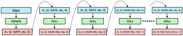
(a) Block Sampling Process

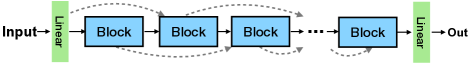
(b) Standard Architecture

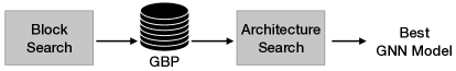
(c) Model Generation Pipline

Figure 2: (a). A example of block sampling process, where $\text{A}_{i}$ and $\text{S}_{j}$ stand for the i-th action and state respectively, and E(S) denotes for the set of valid actions in state S. (b). The standard architecture used for GNN block evaluation. Each block have two inputs, the direct input from previous block and the residual input from the block right before the previous block. (c). Illustration of our proposed GNN generation pipline. More details about the search process are shown in Algorithm 1.

Algorithm 1 DQN for Block-wise search

Given: block-wise space $S_{B}$, DQN agent $DQN_{\theta}$,
block pool $GBP$, memory pool $M$, search epoch $\#_{B}$,
epsilon greedy rate $\epsilon$
Output: Top-k block codes

1:  Initiate $DQN$ parameterized by $\theta$

2:  state = ’start’

3:  for $i=1\to\#_{B}$ do

4:     $\mathbb{C}=[\ ]$

5:     while ’EoB’ not encountered do

6:        rand = random(0,1)

7:        if rand $\leq\epsilon$ then

8:           action = $DQN_{\theta}$(state)  //exploitation

9:        else

10:           action = random_sample(state)  //exploration

11:        end if

12:        state = action

13:        $\mathbb{C}$.append(state)

14:     end while

15:     Build model $M_{\mathbb{C}}$ based on code $\mathbb{C}$

16:     $R_{V}(M_{\mathbb{C}})$ = Evaluate($M_{\mathbb{C}}$)  //train and test model

17:     Update memory pool $P$

18:     Update $\theta$ using $batch$ from $P$ based on Equation (8) and Equation (9)

19:     if $R_{V}(M_{\mathbb{C}})\textgreater min\_acc(GBP)$ then update GBP

20:  end for

21:  return  GBP

3.4 Deep-q-learning Agent

Even after division and pruning, our search space still contains billions of candidate blocks and architectures. For example, when setting the maximum layer number $N_{l}$ to 6, there are approximately $2.047\times 10^{18}$ candidate blocks in the block-wise search space. As GNN model evaluation is time-consuming, it is impossible to iterate over all candidate models. Thus, we need an accurate while sample-efficient search agent to explore the search space. Here, we apply deep-q-learning [23], a variant of Q-learning algorithm, to guide the search over our proposed search space. For better illustration, we use the vanilla Q-learning to describe our agent definitions.

Q-learning is an off-policy reinforcement learning algorithm, which aims at taking the best action $A$ at each step so as to maximize the expected cumulative reward $\mathbb{E}(R)$. There are four key components for q-learning, as agent, environment, state and action. Since we describe our block or architecture using a list of k-D vectors (e.g. k=4 in block-wise search), we define such list of vectors as block/architecture code $\mathbb{C}=[V_{1},V_{2},...,V_{N}]$ where $V_{i}$ denotes for the i-th k-D vectors. To apply Q-learning algorithm to our search process, we consider the sampling of $\mathbb{C}$ as a Markov Decision Process, which means the generation of each k-D vector is probabilistically independent. Based on such presumption, states and actions in Q-learning algorithm could be regarded as the k-D vectors in our search space, while a special ’start’ state is set as the initial state. An example of block-wise sampling process is shown in Figure 2(a). Then, the objective of our agent should be discovering the trajectory $\Gamma_{\mathbb{C}}$ with the highest expected reward:

$$R^{*}=\mathop{argmax}\limits_{\mathbb{C}\in S}(\mathbb{E}[R(\Gamma_{\mathbb{C}})])$$ (6)

Because Q-learning is a kind of Temporal-Difference learning method whose agent could be updated based on an existing estimate, the above objective could be achieved by applying the Bellman Equation recursively. Then, consider time step $t$ and an agent policy $\pi$ , the expected reward in state $S_{t}$ could be written as:

$$R_{\pi}(S_{t}) =\mathbb{E}_{\pi}[\sum_{k=0}^{\infty}\gamma^{k}r_{t+k+1}|S_{t}]$$ (7)

$$=\mathbb{E}_{\pi}[r_{t+1}+\gamma R_{\pi}^{*}(S_{t+1})|S_{t}]$$

where $r_{t}$ is the instant reward obtained when transiting from $S_{t-1}$ to $S_{t}$, and $\gamma$ denotes the discount factor that measures the importance of future expected reward. In Q-learning, each expected reward $R_{\pi}$ in state $S_{t}$ is regarded as a Q-value of state-action pair. Therefore, the above equation could be solved by iteratively updating the Q-value as:

$$Q(S_{t},A_{t})= (1-\alpha)Q(S_{t},A_{t})+$$ (8)

$$\alpha[r_{t+1}+\gamma\max\limits_{A^{\prime}\in E(S_{t})}Q(S_{t+1},A^{\prime})]$$

where $\alpha$ is the learning rate for updating the Q-value, $r_{t+1}$ is the reshaped instant reward which we will discuss later, and $E(S_{t})$ is the set of all valid actions in state $S_{t}$. Additionally, when encountering the last action $A_{T}$, the future expected reward term in Equation (8) is dismissed:

$$Q(S_{T-1},A_{T})=(1-\alpha)Q(S_{T-1},A_{T})+\alpha R_{T}$$ (9)

where $R_{T}$ is the final reward (i.e. model evaluated accuracy $R_{V}(M)$). Note that, because the model could only be constructed and evaluated after the the code $\mathbb{C}$ is generated, the instant reward term $r_{t}$ is hard to decide. Thus, we use reward reshaping [27] to adjust each $r_{t}$ as:

$$r_{t}=R_{T}/\text{len}(\mathbb{C})$$ (10)

Although above definitions make our search agent theoretically feasible, in practice it is unacceptable when applying vanilla q-learning as there are too many states and actions to be stored in q-table. Therefore, we apply two 2-layer MLPs (i.e. deep-q-networks) to approximate the q-table, similar to the deep-q-learning [23]. Meanwhile, as approximating the action-value function often leads to instability [1], we further apply Experience Replay [17, 24] to stabilize the search process. The details will be discussed in the next section. The pseudo code for our guided block-wise search is shown in Algorithm 1. Because of space limitations, we do not present the pseudo code for architecture-wise search, which is similar to block-wise search if we replace $GBP$ in Algorithm 1 with $best\ model$.

Dataset	Cora	CiteSeer	PubMed	CS	Physics	Computer	Photo	Cornell	Texas	Wisconsin
# Nodes	2708	3327	19717	18333	34493	13381	7487	183	183	251
# Edges	5429	4732	44338	81894	247962	245778	119043	295	309	499
# Features	1433	3703	500	6805	8415	767	745	1703	1703	1703
# Classes	7	6	3	15	5	10	8	5	5	5

Table 3: Dataset descriptions.

4 Experiment

In this section, we validate the performance of our proposed method by comparing our auto-generated GNN models against several state-of-the-art graph neural network models on various benchmark datasets. For convenience, our NAS-generated deep GNN model are denoted as Deep-GNAS, while all the directly transferred models and results without researching in the two-stage search space are marked with asterisks.

4.1 Datasets & Experimental Setup

Datasets. We apply our model to 10 open graph benchmarks in Table 3. Settings and descriptions for each dataset will be illustrated under different learning scenarios.

Settings of DQN Agent. To approximate the vanilla q-table, we use two 2-layer MLPs as deep-q-networks, one (i.e. evaluation network) is responsible for mapping the current state to the next action that maximizes future expected reward as in Equation (8), and the other (i.e. target network) is used to train the former MLP with frozen parameters. We update the parameters of target network every 100 search epochs. For the epsilon-greedy sampling, we set the initial exploration rate to 1 and anneal it to zero following cosine decay schedule [21] during the last 60% epochs. To replay the agent memory, we set the memory capacity as 300, and use a batch-size of 32 with future expected reward weight $\gamma=1$. As for the optimizer, we apply Adam [13] with learning rate 0.01. To filter out outstanding GNN models, We set the epoch for block-wise search to 1500 and the size of GNN block pool $GBP$ to 3. After obtaining the top-3 blocks as shown in Figure 3(a), we explore the architecture-wise space for 1000 epochs to discover the best GNN model.

Settings of GNN models. For the block-wise search, we set initial residual connection weight $\alpha=0.3$, identity mapping parameter $\lambda=0.5$, dropout rate $=0.3$. the maximum layer number for each block is set to 6 with hidden size 32. Meanwhile, we use addition for aggregating layer features in a block. Each sampled block is evaluated using the 8-block standard architecture depicted in Figure 2(b), which is trained for 400 epochs using Adam optimizer with learning rate 0.01. Following [6], we set the weight decay for graph convolutional layers to 0.01 and fully connected layers to 4e-5. For the architecture-wise search, the maximum block number is set to 8 while other settings are specified for different datasets.

Type	Method	Cora	CiteSeer	PubMed
	GCN	81.5	71.1	79.0
	GAT	83.1	70.8	78.5
	ARMA	83.4	72.5	78.9
Hand-	APPNP	83.3	71.8	80.1
Crafted	HGCN	79.8 (9)	70.0 (9)	78.4 (9)
	JKNet(Drop)	83.3 (4)	72.6 (16)	79.2 (32)
	Incep(Drop)	83.5 (64)	72.7 (4)	79.5 (4)
	GCNII	85.5 (64)	73.4 (32)	80.2 (16)
	GraphNAS-R	83.3	73.4	79.0
NAS-	GraphNAS	83.7	73.5	80.5
Based	AutoGNN	83.6	73.8	79.7
	DeepGNAS	85.6 (28)	73.6* (31)	81.0* (27)

Table 4: Summary of semi-supervised classification accuracy (%) of different methods on three citation networks. Following [6], the number in parentheses denotes the depth (i.e. layer number) of corresponding GNN model. The results without parentheses are obtained with 2-layer shallow models. And the results with asterisk are obtained using transferred blocks.

Type	Method	Cora	CiteSeer	PubMed	Cornell	Texas	Wisconsin
	GCN	85.77	73.68	88.13	52.70	52.16	45.88
	GAT	86.37	74.32	87.62	54.32	58.38	49.41
	APPNP	87.87	76.53	89.40	73.51	65.41	69.02
	Geom-GCN-I	85.19	77.99	90.05	56.76	57.58	58.24
Hand-Crafted	JKNet	85.25 (16)	75.85 (8)	88.94 (64)	57.30 (4)	56.49 (32)	48.82 (8)
	JKNet(Drop)	87.46 (16)	75.96 (8)	89.45 (64)	61.08 (4)	57.30 (32)	50.59 (8)
	Incep(Drop)	86.86 (8)	76.83 (8)	89.18 (4)	61.62 (16)	57.84 (8)	50.20 (8)
	GCNII	88.49 (64)	77.08 (64)	89.57 (64)	74.86 (16)	69.46 (32)	74.12 (16)
	GCNII†	88.01 (64)	77.13 (64)	90.30 (64)	76.49 (16)	77.84 (32)	81.57 (16)
	GraphNAS	88.40	77.62	88.96	-	-	-
NAS-Based	SNAG	88.95 (3)	76.95 (3)	89.42 (3)	-	-	-
	DeepGNAS*	91.23 (30)	84.04 (31)	90.74 (28)	91.89 (30)	94.59 (30)	95.65 (30)

Table 5: Summary of full-supervised classification accuracy (%) of different methods on three citation networks and three webpage datasets. Following [6], number in parentheses denotes depth (i.e. layer number) of corresponding GNN model. Results without parentheses are obtained with 2-layer shallow models. Note that GCNII^† refers to the GCNII variant proposed in [6]. *Our results are obtained from reused blocks generated from semi-supervised first-stage search on Cora dataset.

4.2 Semi-supervised Learning

In the semi-supervised node classification tasks, we test our model on three Citation networks as Cora, PubMet and CiteSeer. In these datasets, documents are represented as graph nodes and edges correspond to citation links; each node feature corresponds to the bag-of-words representation of the corresponding document while each node correspond to a class label. For fair comparison, we apply the standard training/validation/testing split following [43], where 20 nodes per class are used for training, 500 nodes for validation and 1000 nodes for testing. For baselines, we choose 8 hand-crafted GNN models and 2 NAS-generated models. Among those hand-crafted ones, the first 4 models share shallow 2-layer GNN structures: GCN [14], GAT [40], ARMA [4], APPNP [15]. For the rest manually designed baselines, we follow [6] that equip JKNet [42] and IncepGCN [30] with DropEdge technique, and add one recent hierarchical method HGCN [11], which could serve as deep manual baselines. The metrics are reused as reported in [6] and [7]. Note that unlike previous NAS methods that search for GNN model from scratch on each dataset, we conduct the block-wise search on Cora while transfer the generated blocks in $GBP$ to other datasets, which also leads to competitive results. The results are shown in Table 4. We observe that DeepGNAS achieved best performance on Cora and PubMed while seconding to AutoGNN by 0.2% in CiteSeer dataset. Notably, our model’s accuracy on Cora surpassed all NAS-generated models by about 2%.

Type	Method	CS	Physics	Computer	Photo
	GCN	95.5$\pm$0.3	98.3$\pm$0.2	88.0$\pm$0.6	95.4$\pm$0.3
Hand-	GAT	95.5$\pm$0.3	98.1$\pm$0.2	89.1$\pm$0.6	95.6$\pm$0.3
Crafted	ARMA	95.4$\pm$0.2	98.5$\pm$0.1	86.1$\pm$1.0	94.8$\pm$0.8
	APPNP	95.6$\pm$0.2	98.5$\pm$0.1	89.8$\pm$0.4	95.8$\pm$0.3
NAS-	GraphNAS	97.1$\pm$0.2	98.5$\pm$0.2	92.0$\pm$0.4	96.5$\pm$0.4
Based	DeepGNAS	98.6$\pm$0.3	99.5$\pm$0.3	92.3$\pm$0.5	96.6$\pm$0.2

Table 6: Results of model transferability test in terms of accuracy (%).

4.3 Full-supervised Learning

For the full-supervised learning tasks, we reuse GNN blocks obtained from semi-supervised settings on Cora and only execute the second-stage search on different datasets. We fix some of the hyper-parameters as follows: learning rate = $3\times 10^{-2}$, weight decay for graph convolutional layers = $3\times 10^{-3}$ and hidden dimension = 32. Besides three commonly used citation networks, we further introduce three web page datasets as in [28]: Cornell, Texas and Wisconsin. In these datasets, each node correspond to a web page and edges represent hyperlinks between pages. Node features are the bag-of-words representation of web pages. For fair comparsion, we split all the datasets following [6]: 60% nodes are set for training while 20% for validation and the remaining 20% for testing. We train each model for 400 epochs and report the results in Table 5. The generated architectures correspond to Cora, CiteSeer and Pubmed are depicted in Figure 3(b), 3(c) and 3(d) respectively. The metrics for GCN, GAT and Genom-GCN are reused from [28]. From the results we could observe that our deep GNN model constructed by transferred blocks obtain the highest validation accuracy on all of the 6 datasets. Notably, our proposed method surpasses all other models in the last three datasets by large margin. (i.e. over 14% gain in each of the web page datasets). We assume such performance improvement come from not only our models depth, but also the connection and layer diversity and adaptivity, which is not considered by previous methods. We will further discuss and validate such assumption in section 4.5.

4.4 Model Transferability Test

Even our transferred blocks show competitive performance on various datasets and tasks, we still want to further validate our models capability on pure transfer learning scenarios as proposed by [7]. Thus, in this section, we directly reuse the architecture obtained on citation networks and test it on supervised node classification tasks. Here we apply our model to four datasets: two coauthor datasets as MS-CS and MS-Physics, two product networks as Amazon Computers and Amazon Photo [35]. Following [7], 500 nodes in each dataset are selected for validation, 500 for testing while the remaining nodes are used for training. We also reuse the metrics as reported in [7]. For parameter settings, we set the weight decay and hidden dimension for graph convolutional layers to $3\times 10^{-2}$ and 32 respectively. Each model is trained for 800 epoch using Adam with learning rate 0.06. Classification results are shown in Table 6. We run our model for 10 times and report the mean accuracies with variances. Consequently, our directly transferred GNN model reaches best performance on the four benchmarks, which further demonstrates that transferability not only lies in our generated blocks but also the final architectures.

(a) Generated blocks stored in $GBP$

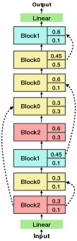
(b) Model-Cora

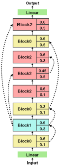
(c) Model-CiteSeer

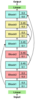
(d) Model-PubMed

Figure 3: (a). Our auto-generated top-3 GNN blocks from block-wise search towards semi-supervised task on Cora. (b), (c) and (d) are best architectures found in full-supervised tasks on Cora, CiteSeer and PubMed respectively.

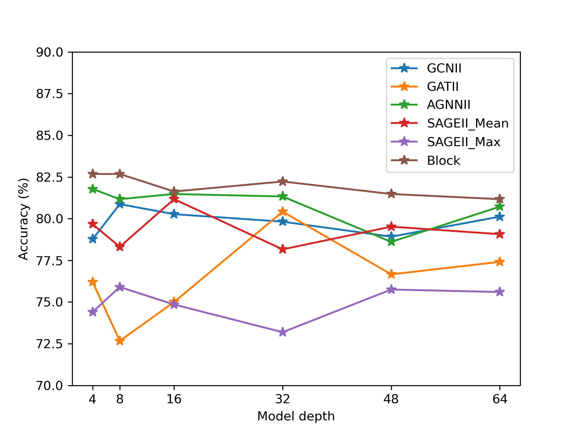
(a) CiteSeer

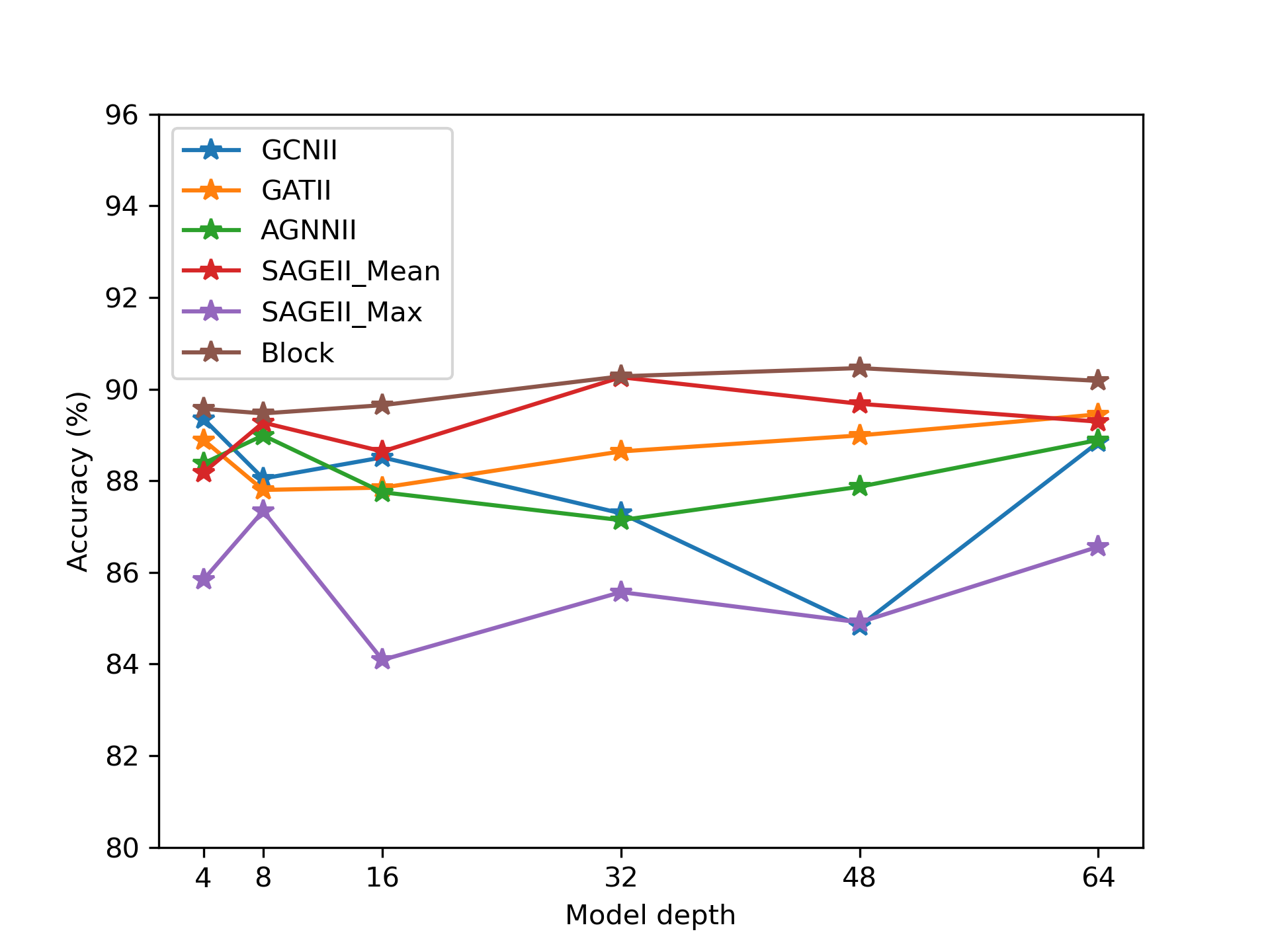
(b) PubMed

Figure 4: Ablation study on structural diversity with model depth increasing from 4 to 64.

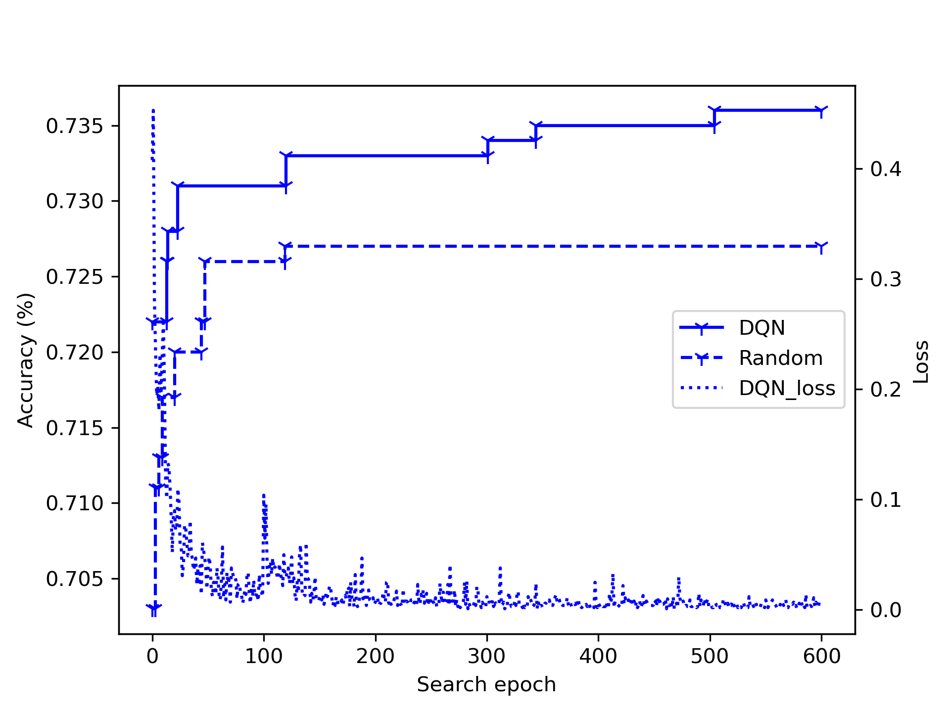
(a) CiteSeer

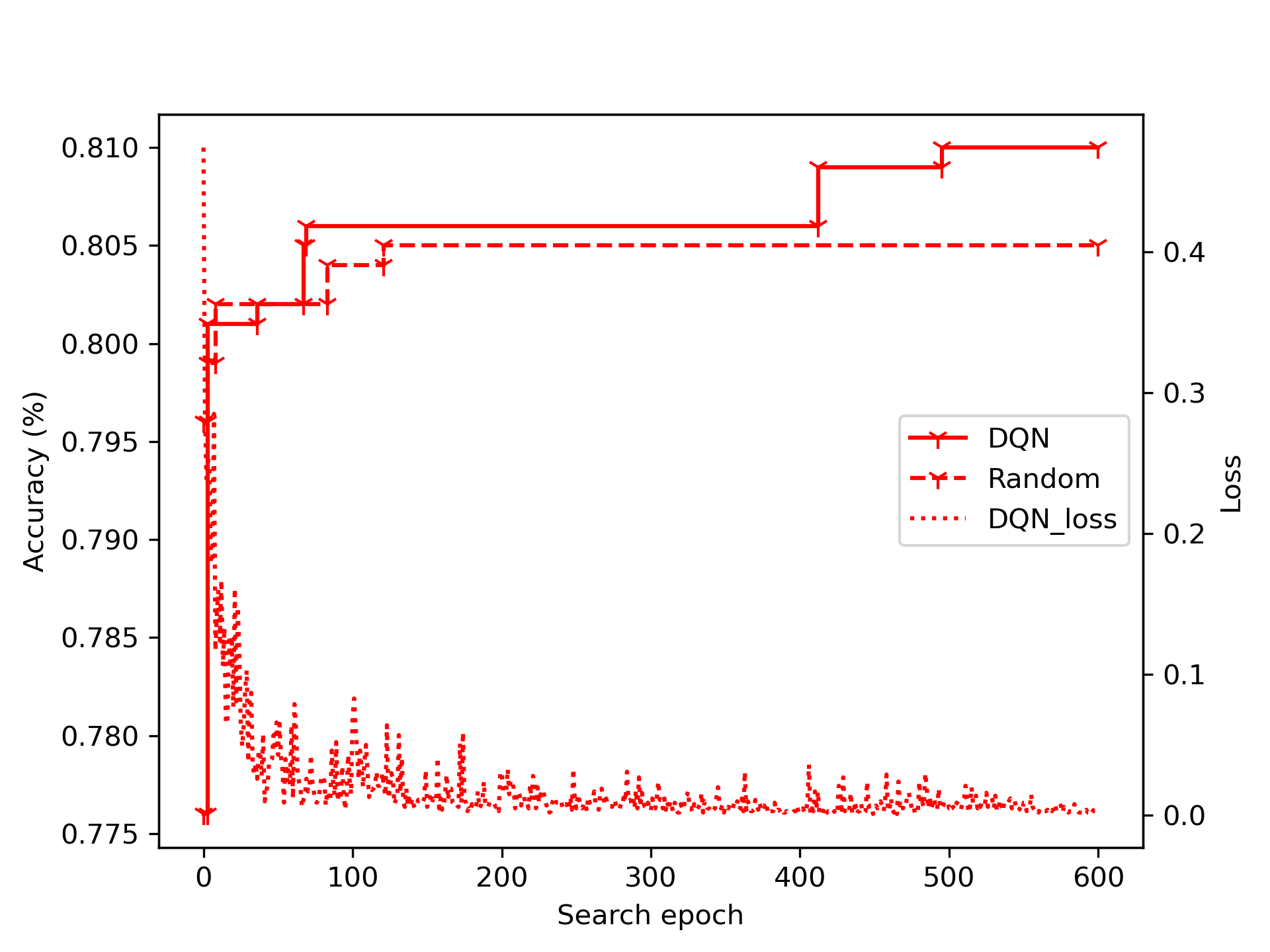
(b) PubMed

Figure 5: Progression of obtained best model with DQN guided search and random search.

4.5 Discussions and ablation studies

Importance of structural diversity. Besides model depth, we assume our model’s superiority comes from the layer diversity and flexibility of connections. To validate this, we conduct ablation study by fixing the layer type and connectivity of final architectures, and then comparing those fixed models with the standard architecture built upon our best block. For fair comparison, we keep hyper-parameters of all models consistent and report the mean accuracy of three independent trainings. As depicted in Figure 4, our generated GNN block could retain stable and good performances when model depth changes, which demonstrates the benefits from structural flexibility and layer diversity.

DQN iteration analysis. Herein we study the effectiveness of our applied DQN reinforcement learning algorithm. We compare it with random search by visualizing the progression of obtained best architectures within a searching period of 600 epochs, alone with the loss of evaluation network in DQN, as depicted in Figure 5. We observe that, in the early stage (i.e. explorations) our DQN agent behaves similarly to random search under the epsilon-greedy strategy. However, after the deep-q-network is sufficiently trained and the exploitation rate grows, our DQN agent could further find more high-performance architectures.

5 Conclusion

In this paper, we study the problem of NAS-based deep graph neural network generations. We initially applied initial residual connection and identity mapping to various graph convolutional layers, and present a novel block-wise deep graph neural network generation pipeline. To efficiently explore the exponentially growing search space, we divide the overall search into two stages and utilize a deep-q-learning agent to guide the search process. In experiments, our generated deep GNN models reach state-of-the-art performance on various datasets and learning scenarios. Moreover, both our generated blocks and architectures show great transferability toward new datasets.

References

- [1] Leemon Baird. Residual algorithms: Reinforcement learning with function approximation. In Machine Learning Proceedings 1995, pages 30–37. Elsevier, 1995.
- [2] Bowen Baker, Otkrist Gupta, Nikhil Naik, and Ramesh Raskar. Designing neural network architectures using reinforcement learning. In ICLR (Poster). OpenReview.net, 2017.
- [3] Peter W. Battaglia, Razvan Pascanu, Matthew Lai, Danilo Jimenez Rezende, and Koray Kavukcuoglu. Interaction networks for learning about objects, relations and physics. In NIPS, pages 4502–4510, 2016.
- [4] Filippo Maria Bianchi, Daniele Grattarola, Lorenzo Livi, and Cesare Alippi. Graph neural networks with convolutional ARMA filters. CoRR, abs/1901.01343, 2019.
- [5] Deli Chen, Yankai Lin, Wei Li, Peng Li, Jie Zhou, and Xu Sun. Measuring and relieving the over-smoothing problem for graph neural networks from the topological view. In AAAI, pages 3438–3445. AAAI Press, 2020.
- [6] Ming Chen, Zhewei Wei, Zengfeng Huang, Bolin Ding, and Yaliang Li. Simple and deep graph convolutional networks. In ICML, volume 119 of Proceedings of Machine Learning Research, pages 1725–1735. PMLR, 2020.
- [7] Yang Gao, Hong Yang, Peng Zhang, Chuan Zhou, and Yue Hu. Graph neural architecture search. In IJCAI, pages 1403–1409. ijcai.org, 2020.
- [8] M. Gori, G. Monfardini, and F. Scarselli. A new model for learning in graph domains. In Proceedings. 2005 IEEE International Joint Conference on Neural Networks, 2005., volume 2, pages 729–734 vol. 2, 2005.
- [9] William L. Hamilton, Zhitao Ying, and Jure Leskovec. Inductive representation learning on large graphs. In NIPS, pages 1024–1034, 2017.
- [10] Kaiming He, Xiangyu Zhang, Shaoqing Ren, and Jian Sun. Deep residual learning for image recognition. In CVPR, pages 770–778. IEEE Computer Society, 2016.
- [11] Fenyu Hu, Yanqiao Zhu, Shu Wu, Liang Wang, and Tieniu Tan. Hierarchical graph convolutional networks for semi-supervised node classification. In IJCAI, pages 4532–4539. ijcai.org, 2019.
- [12] Daniel D. Johnson. Learning graphical state transitions. In ICLR. OpenReview.net, 2017.
- [13] Diederik P. Kingma and Jimmy Ba. Adam: A method for stochastic optimization. In ICLR (Poster), 2015.
- [14] Thomas N. Kipf and Max Welling. Semi-supervised classification with graph convolutional networks. In ICLR (Poster). OpenReview.net, 2017.
- [15] Johannes Klicpera, Aleksandar Bojchevski, and Stephan Günnemann. Predict then propagate: Graph neural networks meet personalized pagerank. In ICLR (Poster). OpenReview.net, 2019.
- [16] Guohao Li, Matthias Müller, Ali K. Thabet, and Bernard Ghanem. Deepgcns: Can gcns go as deep as cnns? In ICCV, pages 9266–9275. IEEE, 2019.
- [17] Long-Ji Lin. Reinforcement Learning for Robots Using Neural Networks. PhD thesis, 1992. UMI Order No. GAX93-22750.
- [18] Chenxi Liu, Barret Zoph, Maxim Neumann, Jonathon Shlens, Wei Hua, Li-Jia Li, Li Fei-Fei, Alan L. Yuille, Jonathan Huang, and Kevin Murphy. Progressive neural architecture search. In ECCV (1), volume 11205 of Lecture Notes in Computer Science, pages 19–35. Springer, 2018.
- [19] Hanxiao Liu, Karen Simonyan, and Yiming Yang. DARTS: differentiable architecture search. In ICLR (Poster). OpenReview.net, 2019.
- [20] Xiao Liu, Zhunchen Luo, and Heyan Huang. Jointly multiple events extraction via attention-based graph information aggregation. In EMNLP, pages 1247–1256. Association for Computational Linguistics, 2018.
- [21] Ilya Loshchilov and Frank Hutter. SGDR: stochastic gradient descent with warm restarts. In ICLR (Poster). OpenReview.net, 2017.
- [22] Sitao Luan, Mingde Zhao, Xiao-Wen Chang, and Doina Precup. Break the ceiling: Stronger multi-scale deep graph convolutional networks. In NeurIPS, pages 10943–10953, 2019.
- [23] Volodymyr Mnih, Koray Kavukcuoglu, David Silver, Andrei A. Rusu, Joel Veness, Marc G. Bellemare, Alex Graves, Martin A. Riedmiller, Andreas Fidjeland, Georg Ostrovski, Stig Petersen, Charles Beattie, Amir Sadik, Ioannis Antonoglou, Helen King, Dharshan Kumaran, Daan Wierstra, Shane Legg, and Demis Hassabis. Human-level control through deep reinforcement learning. Nat., 518(7540):529–533, 2015.
- [24] Volodymyr Mnih, Koray Kavukcuoglu, David Silver, Andrei A Rusu, Joel Veness, Marc G Bellemare, Alex Graves, Martin Riedmiller, Andreas K Fidjeland, Georg Ostrovski, et al. Human-level control through deep reinforcement learning. nature, 518(7540):529–533, 2015.
- [25] Federico Monti, Michael M. Bronstein, and Xavier Bresson. Geometric matrix completion with recurrent multi-graph neural networks. In NIPS, pages 3697–3707, 2017.
- [26] Niv Nayman, Asaf Noy, Tal Ridnik, Itamar Friedman, Rong Jin, and Lihi Zelnik-Manor. XNAS: neural architecture search with expert advice. In NeurIPS, pages 1975–1985, 2019.
- [27] Andrew Y. Ng, Daishi Harada, and Stuart J. Russell. Policy invariance under reward transformations: Theory and application to reward shaping. In ICML, pages 278–287. Morgan Kaufmann, 1999.
- [28] Hongbin Pei, Bingzhe Wei, Kevin Chen-Chuan Chang, Yu Lei, and Bo Yang. Geom-gcn: Geometric graph convolutional networks. In ICLR. OpenReview.net, 2020.
- [29] Hieu Pham, Melody Y. Guan, Barret Zoph, Quoc V. Le, and Jeff Dean. Efficient neural architecture search via parameter sharing. In ICML, volume 80 of Proceedings of Machine Learning Research, pages 4092–4101. PMLR, 2018.
- [30] Yu Rong, Wenbing Huang, Tingyang Xu, and Junzhou Huang. Dropedge: Towards deep graph convolutional networks on node classification. In ICLR. OpenReview.net, 2020.
- [31] Emanuele Rossi, Fabrizio Frasca, Ben Chamberlain, Davide Eynard, Michael M. Bronstein, and Federico Monti. SIGN: scalable inception graph neural networks. CoRR, abs/2004.11198, 2020.
- [32] Alvaro Sanchez-Gonzalez, Nicolas Heess, Jost Tobias Springenberg, Josh Merel, Martin A. Riedmiller, Raia Hadsell, and Peter W. Battaglia. Graph networks as learnable physics engines for inference and control. In ICML, volume 80 of Proceedings of Machine Learning Research, pages 4467–4476. PMLR, 2018.
- [33] J. D. Schaffer, D. Whitley, and L. J. Eshelman. Combinations of genetic algorithms and neural networks: a survey of the state of the art. In [Proceedings] COGANN-92: International Workshop on Combinations of Genetic Algorithms and Neural Networks, pages 1–37, 1992.
- [34] Sungyong Seo, Chuizheng Meng, and Yan Liu. Physics-aware difference graph networks for sparsely-observed dynamics. In ICLR. OpenReview.net, 2020.
- [35] Oleksandr Shchur, Maximilian Mumme, Aleksandar Bojchevski, and Stephan Günnemann. Pitfalls of graph neural network evaluation. CoRR, abs/1811.05868, 2018.
- [36] K. O. Stanley, D. B. D’Ambrosio, and J. Gauci. A hypercube-based encoding for evolving large-scale neural networks. Artificial Life, 15(2):185–212, 2009.
- [37] Kenneth O. Stanley and Risto Miikkulainen. Evolving neural networks through augmenting topologies. Evolutionary Computation, 10(2):99–127, 2002.
- [38] Masanori Suganuma, Shinichi Shirakawa, and Tomoharu Nagao. A genetic programming approach to designing convolutional neural network architectures. In IJCAI, pages 5369–5373. ijcai.org, 2018.
- [39] Christian Szegedy, Wei Liu, Yangqing Jia, Pierre Sermanet, Scott E. Reed, Dragomir Anguelov, Dumitru Erhan, Vincent Vanhoucke, and Andrew Rabinovich. Going deeper with convolutions. In CVPR, pages 1–9. IEEE Computer Society, 2015.
- [40] Petar Velickovic, Guillem Cucurull, Arantxa Casanova, Adriana Romero, Pietro Liò, and Yoshua Bengio. Graph attention networks. In ICLR (Poster). OpenReview.net, 2018.
- [41] Keyulu Xu, Weihua Hu, Jure Leskovec, and Stefanie Jegelka. How powerful are graph neural networks? In ICLR. OpenReview.net, 2019.
- [42] Keyulu Xu, Chengtao Li, Yonglong Tian, Tomohiro Sonobe, Ken-ichi Kawarabayashi, and Stefanie Jegelka. Representation learning on graphs with jumping knowledge networks. In ICML, volume 80 of Proceedings of Machine Learning Research, pages 5449–5458. PMLR, 2018.
- [43] Zhilin Yang, William W. Cohen, and Ruslan Salakhutdinov. Revisiting semi-supervised learning with graph embeddings. In ICML, volume 48 of JMLR Workshop and Conference Proceedings, pages 40–48. JMLR.org, 2016.
- [44] Rex Ying, Ruining He, Kaifeng Chen, Pong Eksombatchai, William L. Hamilton, and Jure Leskovec. Graph convolutional neural networks for web-scale recommender systems. In Proceedings of the 24th ACM SIGKDD International Conference on Knowledge Discovery & Data Mining, KDD 2018. ACM, 2018.
- [45] Victoria Zayats and Mari Ostendorf. Conversation modeling on reddit using a graph-structured LSTM. Trans. Assoc. Comput. Linguistics, 6:121–132, 2018.
- [46] Huan Zhao, Lanning Wei, and Quanming Yao. Simplifying architecture search for graph neural network. In CIKM (Workshops), volume 2699 of CEUR Workshop Proceedings. CEUR-WS.org, 2020.
- [47] Zhao Zhong, Junjie Yan, Wei Wu, Jing Shao, and Cheng-Lin Liu. Practical block-wise neural network architecture generation. In CVPR, pages 2423–2432. IEEE Computer Society, 2018.
- [48] Kuangqi Zhou, Yanfei Dong, Kaixin Wang, Wee Sun Lee, Bryan Hooi, Huan Xu, and Jiashi Feng. Understanding and resolving performance degradation in graph convolutional networks, 2020.
- [49] K. Zhou, Qingquan Song, Xiao Huang, and X. Hu. Auto-gnn: Neural architecture search of graph neural networks. ArXiv, abs/1909.03184, 2019.
- [50] Barret Zoph and Quoc V. Le. Neural architecture search with reinforcement learning. In ICLR. OpenReview.net, 2017.