Weakly first-order quantum phase transition between Spin Nematic and Valence Bond Crystal Order in a square lattice SU(4) fermionic model

Abstract

We consider a model Hamiltonian with two SU$(4)$ fermions per site on a square lattice, showing a competition between bilinear and biquadratic interactions. This model has generated interest due to possible realizations in ultracold atom experiments and existence of spin liquid ground states. Using a basis transformation, we show that part of the phase diagram is amenable to quantum Monte Carlo simulations without a sign problem. We find evidence for spin nematic and valence bond crystalline phases, which are separated by a weak first order phase transition. A U($1$) symmetry is found to emerge in the valence bond crystal histograms, suggesting proximity to a deconfined quantum critical point. Our results are obtained with the help of a loop algorithm which allows large-scale simulations of bilinear-biquadratic SO($N$) models on arbitrary lattices in a certain parameter regime.

Introduction – Extended symmetries often offer a way to realize new phases of matter in simple models of strongly correlated quantum systems. An important motivation for extended symmetries comes from studying the limit where the number of internal degrees of freedom $N$ becomes large, an ubiquitous tool in theoretical physics Stanley (1968); Hooft (1974); Moshe and Zinn-Justin (2003). Indeed this large-$N$ limit is often tractable analytically, allowing a better physical understanding and giving a starting point for an expansion aimed to characterize the small-$N$, physical, cases. In quantum magnetism, this approach was pionereed by enlarging the symmetry group to SU$(N)$ where it was for instance predicted, using field-theoretical analysis Read and Sachdev (1989, 1990), that the well-known antiferromagnetic (Néel) ordered phase present on the square lattice at small $N$ is replaced by a valence-bond crystal (VBC) that breaks lattice symmetries at large $N$. For several SU$(N)$ representations and different lattices, numerical studies have confirmed the existence of ground-states without magnetic long-range order Harada et al. (2003); Corboz et al. (2011, 2012a, 2012b, 2013); Nataf et al. (2016). Extended symmetries are not only useful as a theoretical knob, but are also meaningful to describe experimental systems: for instance, SU$(4)$ symmetry is relevant for materials with strong spin-orbit coupling Kugel’ and Khomskiĭ (1982); Yamada et al. (2018) while SO$(4)$ symmetry has been suggested for twisted bilayer graphene You and Vishwanath (2019). In atomic physics, alkaline-earth ultracold atoms show an almost perfect realization of SU$(N)$ symmetry groups with high values of $N$ Cazalilla and Rey (2014); Gorshkov et al. (2010); Pagano et al. (2014); DeSalvo et al. (2010); Tey et al. (2010); Taie et al. (2010) while spin-3/2 fermions can realize SO(5) symmetry Wu et al. (2003); Wu (2006). Recent experiments with ultracold atomic systems show that low temperatures can be reached for SU(N)-symmetric alkaline-earth elements Sonderhouse et al. (2020) while a filling of two fermions per site can be realized Hartke et al. (2022) as it avoids three-body losses.

The competition between different energy terms, compatible with extended symmetries, is another fruitful approach to engineer unconventional phenomena Kaul et al. (2013). For instance, the competition between VBC and Néel ordered phases found in large-$N$ theories triggered a large interest due to the possibility of a generically continuous deconfined quantum critical point (DQCP) Senthil et al. (2004a, b); Sandvik (2007) between these two phases of matter, in contradiction with naive expectations from Landau-Ginzburg theory. A continuous transition can be observed numerically by either artificially treating $N$ as a continuous parameter Beach et al. (2009a), or due to the competition between terms involving two and four or more spins, for a large variety of SU$(2)$ and SU$(N)$ models Kaul (2011); Harada et al. (2013); Kaul and Sandvik (2012); Sandvik (2007, 2010); Lou et al. (2009). An excellent agreement with large-$N$ DQCP predictions is obtained as $N$ is increased Kaul and Sandvik (2012). For magnetic systems hosting spins larger than $1/2$, another important competing term compatible with SU$(N\geq 2)$ symmetry is a biquadratic coupling between two spins. Biquadratic terms are also relevant for cold-atomic systems Yip (2003); Imambekov et al. (2003); Eckert et al. (2007); Brennen et al. (2007); Puetter et al. (2008). For spin-1 systems in two dimensions (2D), it is possible to obtain a (spin) nematic (or ferroquadrupolar) ground-state that breaks SU$(2)$ symmetry, without any local magnetization, but with a finite quadrupolar order Penc and Läuchli . For instance, the bilinear-biquadratic Heisenberg model on the square lattice exhibits a very rich phase diagram Papanicolaou (1988); Tóth et al. (2012); Niesen and Corboz (2017), including a nematic phase. For a quasi-one-dimensional spin-1 model, Harada et al. Harada et al. (2006) found numerical evidence for a continuous transition between a nematic and a VBC phase. The VBC phase does not survive to the isotropic 2D limit, leading instead to a magnetically ordered phase which exhibits a first-order transition to the nematic phase. This system was analyzed with a bond-operator treatment in Ref. Puetter et al. (2008), predicting a generic first-order nematic-VBC transition, along with a discussion of possible spin liquid behavior for SO$(N)$ symmetry at large $N$. On the other hand, a general discussion of nematic behavior from the perspective of a continuum field theory incorporating the role of Berry phases Grover and Senthil (2007) allows for a continuous DQCP to a VBC phase for quasi-one-dimensional SO$(3)$ models. In a subsequent quantum Monte Carlo (QMC) numerical study, Kaul Kaul (2012) showed that a pure biquadratic model on a triangular lattice, which is known to host a nematic ground-state and has an extended SO$(3)$ symmetry Läuchli et al. (2006); Kaul (2012), can exhibit VBC or spin-liquid ground-states when the symmetry is extended to SO$(N)$ for large-enough $N$ and/or in presence of further competing interactions Kaul (2015). The phase transitions between spin nematic and VBC phases were found to be discontinuous.

In this work, we consider a square lattice model built out of two SU$(4)$ fermions per site, showing a competition between bilinear and biquadratic terms. This model has been discussed earlier Marston and Affleck (1989); Affleck et al. (1991); Paramekanti and Marston (2007); Gauthé et al. (2020); Kim et al. (2019); Wang et al. (2014a) with predictions of a rich phase diagram with Néel order, VBC, ferromagnet and charge-conjugation symmetry broken phases Paramekanti and Marston (2007), as well as of critical spin liquids phases from a projected entangled pair states (PEPS) ansatz Gauthé et al. (2020). We use an exact mapping to an SO$(n_{c})$ model with $n_{c}=6$ colors, and show that part of the phase diagram can be simulated exactly using QMC with no sign problem.

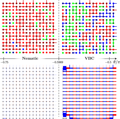
Figure 1: Phase diagram in the sign-free region $\{\theta_{\rm SF}\}=[-3/4\pi,-\pi/2]$: Nematic to VBC transition for $\theta_{c}=-0.5969(1)\pi$. Upper panels : representative configurations (see text) constructed from snapshots of Monte Carlo configurations. Bottom panels : real-space pattern of the connected bond correlator $D_{\rm corr}(b)-D_{\rm corr}^{\rm avg}$ with respect to the bottom left bond (shown in black). Blue and red mean positive and negative respectively and the bond thickness denotes the magnitude. Data are presented for $\theta=-0.74\pi$ (nematic) and $\theta=-0.5\pi$ (VBC).

Model definitions – We first define the model with two SU$(4)$ fermions per lattice site, which form a 6-dimensional space at each site Marston and Affleck (1989); Affleck et al. (1991); Paramekanti and Marston (2007); Gauthé et al. (2020), with the following Hamiltonian

$${\cal H}=J\sum_{\langle ij\rangle}{\bf S}_{i}\cdot{\bf S}_{j}+\frac{K}{4}\sum_{\langle ij\rangle}({\bf S}_{i}\cdot{\bf S}_{j})^{2},$$ (1)

where $J=\cos(\theta)$ and $K=\sin(\theta)$. By analogy with the usual SU($2$) spin case, the 15-dimensional vector ${\bf S}$ is formed by the generators of SU($4$) and the “spin” interaction ${\bf S}\cdot{\bf S}$ can be expressed as a linear combination of symmetric projectors on different irreducible on-site representations (see Ref. Gauthé et al. (2020)). The model exhibits an enlarged SU($6$) symmetries at $J=0$ ($\theta=\pm\pi/2$, with fundamental representation on one sublattice and conjugate on the other one) and $J=K$ ($\theta=-3/4\pi$,  $\pi/4$, with fundamental representation on each lattice site). QMC studies of the Hubbard model at large interaction find a critical or weakly ordered Néel phase Assaad (2005); Wang et al. (2014b) at $\theta=0$. The Hamiltonian can be alternatively written in a basis with $n_{c}=6$ colors degree of freedom ($c=1\ldots 6$), encoding the six possible states on each site (see Sup. Mat. sup ). Denoting by $\bar{c}=n_{c}+1-c$ the complementary color of $c$, the Hamiltonian reads (up to an irrelevant constant):

$${\cal H}=\sum_{\langle i,j\rangle}\sum_{c,c^{\prime}}\left(J|cc^{\prime}\rangle\langle c^{\prime}c|+(K-J)|c\bar{c}\rangle\langle c^{\prime}\bar{c^{\prime}}|\right).$$ (2)

In this form, the model has non-positive matrix elements when $J\leq 0$ and $K\leq J$, resulting in the sign-problem free region $\{\theta_{\rm SF}\}=[-3/4\pi,-\pi/2]$ for QMC simulations in this color basis. A variational wave-function analysis Paramekanti and Marston (2007) predicts the existence of a VBC (dimerized) and ferromagnetic phases in this region. Quite interestingly, PEPS computations Gauthé et al. (2020) find in the same region indications for a lack of ordering, and two variational (critical) spin liquids wave-functions with very competitive energies. We adapt (see details in Sup. Mat.sup ) an efficient QMC loop algorithm for bilinear-biquadratic spin 1 models Kawashima and Harada (2004), to simulate the model Eq. 4 in $\{\theta_{\rm SF}\}$. We perform simulations of square lattice samples with $N=L^{2}$ sites with linear size $L$ up to $96$, and up to inverse temperature $\beta=2L$ in units of $1/\sqrt{J^{2}+K^{2}}$ to reach ground-state properties. Our results can be summarized as follows (see Fig. 1). We find that the region $\{\theta_{\rm SF}\}$ hosts two ordered phases: a VBC phase (known Harada et al. (2003) to exist at $\theta=-\pi/2$) as well as a nematic phase defined by a spontaneous symmetry-breaking choice of color pairs, which appears to have been missed earlier. Cartoon representations of QMC configuration snapshots for these two phases are provided in Fig. 1, where states $c$ and $\bar{c}$, which form a nematic pair, are represented by different shades of the same color, and bonds of the same color are drawn between neighboring lattice sites hosting $c$ and $\bar{c}$. In the nematic phase, one of three possible colors dominates, whereas in the VBC phase, there is no dominance of a single color, but most neighboring lattice sites are connected by bonds. The VBC pattern is not easily discernible and a more detailed study of the dimer correlation in the VBC phase is presented later in this manuscript. We provide evidence for a very weak first-order transition between the VBC and the nematic phase at $\theta_{c}=-0.5969(1)\pi$. The VBC phase is furthermore found to exhibit an emergent U$(1)$ behavior all along the range $[\theta_{c},-\pi/2]$ amenable to QMC, restricting our ability to classify this phase into columnar, plaquette or mixed order Ralko et al. (2008); Yan et al. (2021). This emerging symmetry is strongly reminiscent of the behavior observed at or close to a DQCP Sandvik (2007); Jiang et al. (2008); Lou et al. (2009); Sandvik (2012); Nahum et al. (2015); Pujari et al. (2013); Sreejith et al. (2019). We suggest that our results could correspond to a runaway flow close to a potential DQCP fixed point, similar to the theory between nematic and VBC phases presented by Grover and Senthil Grover and Senthil (2007) for an SO$(3)$ quasi-one-dimensional model, calling for a similar analysis for the SO$(6)$ case.

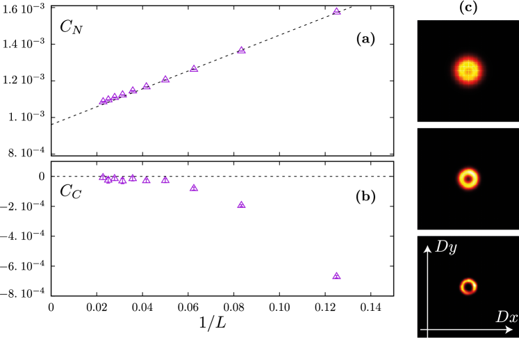
Figure 2: (a) Nematic correlator $C_{N}$ at separation $(L/2,L/2)$, extrapolated to a non-zero value of $9.61(1)\times 10^{-4}$ in the thermodynamic limit for $\theta=-0.65\pi$ as a function of inverse size $1/L$. (b) Same for the cartan correlation at separation $(L/2,L/2)$, see to vanish for $1/L\to 0$. (c) VBC histograms for sizes 16, 32 and 64 at $\theta=-0.5\pi$.

Long-range ordered phases – To motivate the presence of nematic ordering in the range $\theta\in[-0.75\pi,\theta_{c}]$, we present Cartan and nematic correlation functions (defined below) for a system of linear size $L$. We use three Cartan operators $C_{\alpha=1,2,3}=\sum_{c}b^{c}_{\alpha}|c\rangle\langle c|$ with $b_{1}=\frac{1}{2}(1,1,0,0,-1,-1),b_{2}=\frac{1}{2}(-1,0,1,-1,0,1),b_{3}=\frac{1}{2}(1,-1,0,0,1,-1)$ corresponding to the underlying SU$(4)$ symmetry and diagonal in the color basis, forming the vector ${\bf C}=(C_{1},C_{2},C_{3})$ at any site. To identify simple (anti-)ferromagnetic ordering, we consider the Cartan correlator $C_{C}=\braket{{\bf C}_{{\bf r}=(0,0)}\cdot{\bf C}_{{\bf r}=(L/2,L/2)}}$, whereas $C_{N}=\braket{Q_{1,{\bf r}=(0,0)}Q_{1,{\bf r}=(L/2,L/2)}}$, with the traceless operator $Q_{1}=C_{1}C_{1}-\frac{1}{6}$, is used to identify nematic ordering. Details about the choice of Cartan operators and connections to the spin operators of SU$(4)$ are provided in Sup. Mat. sup, .

Large size behaviors of these correlators are displayed in Fig. 2(a,b) for $\theta=-0.65\pi$ (located in the nematic phase and relatively away from the critical point), where we clearly see that there is long-range ordering in the nematic correlator but not in the Cartan correlator. We now turn to the VBC phase, which we first illustrate by the real space pattern (Fig. 1) of dimer correlations, defined as $D_{\rm corr}(b)=\braket{({\bf C}_{0,0}\cdot{\bf C}_{1,0})({\bf C}_{\vec{r}^{b}_{1}}\cdot{\bf C}_{\vec{r}^{b}_{2}})}$. Here $b$ indicates a bond number connecting nearest neighbor sites $\vec{r}^{\;b}_{1}$ and $\vec{r}^{\;b}_{2}$. Data in Fig. 1 are taken at the SU($6$) point $\theta=-0.5\pi$ where previous simulations Harada et al. (2003) showed the existence of long-range VBC order, but without specification of the type of crystal encountered. Note that we only present the connected correlation function, i.e. the value $D_{\rm corr}^{\rm avg}=\frac{1}{N_{b}}\sum_{b}D_{\rm corr}(b)$ is subtracted out to only show the non-trivial features. An analysis of the pattern in Fig. 1 along the lines of Ref. Mambrini et al., 2006 reveals that it is different from the one expected in a pristine columnar state, but potentially compatible with plaquette order. We provide next a detailed analysis of the symmetry of the VBC ordering.

Emergence of a $U(1)$ symmetry – For this, we define a vector order parameter ${\bf D}=(D_{x},D_{y})$ with $D_{x}=\sum_{i}(-1)^{i_{x}}C_{i_{x},i_{y}}\cdot C_{i_{x}+1,i_{y}}$ and $D_{y}=\sum_{i}(-1)^{i_{y}}C_{i_{x},i_{y}}\cdot C_{i_{x},i_{y}+1}$. We can build a 2D-histogram of ${\bf D}$ using the spatial configurations generated in the QMC sampling. This is shown for the same parameter values as in Fig. 2 where we clearly see a U$(1)$ symmetry emerging. A similar U$(1)$ symmetry is often observed for VBC phases close to DQCP Sandvik (2007, 2012); Nahum et al. (2015); Pujari et al. (2013) but is generically not expected at the coexistence point between phases at a first order transition (see however recent works Zhao et al. (2019); Serna and Nahum (2019); Takahashi and Sandvik (2020)). We find a finite order parameter for VBC order (characterized by a finite radius in Fig. 2) and a U$(1)$ symmetry (circular shape in Fig. 2) in the entire range $[\theta_{c},-\pi/2]$ on the system sizes accessible to us. We expect that eventually on larger sizes the histograms would show peaks at specific angles characteristic of the type of crystal ordering (e.g. at $0,\pm\pi/2,\pi$ for columnar order), but we are unable to reach this behavior. In the Sup. Mat.sup , we present an analysis of the persistence of this U$(1)$ behavior for large $L$. We also expect the VBC to subsist for $\theta>-\pi/2$, even though it is difficult to pinpoint where it vanishes as QMC is not longer available.

Weak first-order transition – We now present evidence for a weak first-order transition between the nematic and VBC phases. Its weak nature makes it difficult to probe numerically, as several standard indications of a continuous phase transition are observed on small to intermediate length scales, as we now show. As the nematic phase breaks a continuous SO$(6)$ symmetry, it is illuminating to carry out simulations in a basis where the symmetry is made explicit. We call this basis the nematic basis (denoted by ${{\mathbb{N}}}$) which is related to the sign-free color basis as follows: $\ket{c}=\frac{1}{\sqrt{2}}(\ket{\mathbb{N}_{c}}-i\ket{\mathbb{N}_{\bar{c}}}),\ket{\bar{c}}=\frac{1}{\sqrt{2}}(\ket{\mathbb{N}_{c}}+i\ket{\mathbb{N}_{\bar{c}}})$. The Hamiltonian in this basis and the explicit $SO(6)$ symmetry are detailed in Sup. Mat. sup . We can then define a 6-dimensional nematic order parameter $M^{c}=\frac{1}{N}(\sum_{i}\ket{{{\mathbb{N}}}_{c}}\bra{{{\mathbb{N}}}_{c}})-\frac{1}{6}$, corresponding to ”ferromagnetic” ordering in this basis. The VBC ordering is quantified by the amplitude of the VBC order parameter ${\bf D}^{2}=D_{x}^{2}+D_{y}^{2}$.

Given these order parameters, a traditional way of inquiring about the order of the phase transition is to consider their Binder cumulants. We find (see Sup. Mat. sup ) that while they clearly indicate the existence of long-range order away from the critical point, Binder cumulants have a non-monotonic behavior near $\theta_{c}$ which prevents for a conclusive determination of the nature of the phase transition. We further consider the nematic “color” stiffness $\rho_{c}$ defined using the spatial winding of loops in the QMC simulation as $\rho_{c}=\frac{1}{2}\braket{\sum_{\alpha=x,y}\sum_{i}(W^{\alpha}_{i})^{2}}/\beta$, where $i$ runs over all the loops in a particular space-time configuration. The spatial winding $W^{\alpha}_{i}$ of a particular loop $i$ is an integer counting how many sites it wraps over the periodic boundary conditions of the system in the direction $\alpha$. This definition follows from a similar treatment of an SO$(3)$ system Kaul (2012). We expect this stiffness to be finite in the nematic phase, to vanish in the VBC phase and to scale as $L^{-z}$ (with $z$ the dynamical critical exponent) at a continuous phase transition. Fig. 3 reveals a crossing of curves for different system sizes when rescaling the stiffness by $L$, which would be a signature of a continuous phase transition with $z=1$ close to $\theta\simeq-0.5969(1)\pi$. This behavior is seen up to length scales of $L=36$. Further evidence for behavior consistent with a continuous transition is provided by studies of the second derivative of the local energy in Sup. Mat. sup up to $L=36$ along with an estimate for the correlation length (effective) critical exponent $\nu$. Detailed histograms for $L=32$ for the energy, nematic and VBC order parameters are also presented in Sup. Mat. sup showing no discernible signatures of coexistence and hence compatible with a continuous transition up to this length scale.

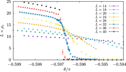
Figure 3: Nematic stiffness scaling across the transition. Here $\beta=2L$.

However, for larger sizes, we find a clear coexistence of both phases at the transition. This is shown in Fig. 4 through a Monte Carlo time trace of the QMC data for a system with $L=40$. It can be seen that the system transits abruptly between the two phases, consistent with the expectation for a first order transition. We have also simulated system sizes up to $L=72$ and find that the jumps between phases become increasingly unlikely with increasing size. Note that the largest value that $(D_{x}^{2}+D_{y}^{2})$ can take is $1$ for perfect VBC ordering, compared to the value of $\approx 0.007$ taken at the transition. This indicates that the transition is only weakly first order and that it cannot be identified for smaller sizes. Note that as the nematic phase breaks a continuous symmetry, the values for ${\bf M}^{2}$ show a spread in Fig. 4 but also in the nematic phase. In the Sup. Mat. sup , we also provide a comparison with the same transition occurring for the model Eq. 4 with $5$ colors, corresponding to an $SO(5)$ symmetry.

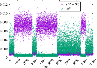
Figure 4: Monte Carlo time series of the (square of the) order parameters at the best estimate for the phase transition ($\theta=-0.5969\pi$) for $L=40$ and $\beta/L=0.4$.

Conclusion and perspectives – In conclusion, using large-scale unbiased QMC simulations, we have shown the existence of a spin nematic phase bordered by a VBC phase (for $\theta>\theta_{c}$) and a ferromagnetic phase $(\theta<-3/4\pi)$ in a system of SU$(4)$ fermions with two particles per site. While the ferromagnetic/nematic transition is strongly first order (level crossings can be observed in exact diagonalization of small clusters Gauthé et al. (2020)), we showed that the transition between nematic and VBC phases is weakly first-order. The relevance of biquadratic terms in cold-atomic systems Yip (2003); Imambekov et al. (2003); Eckert et al. (2007); Brennen et al. (2007); Puetter et al. (2008) suggests that this model and its corresponding quantum phase transition can be realized in ultracold atomic setups. Note that a spin nematic phase has been observed in spin-1 spinor condensates Zibold et al. (2016). The field theory analysis of Ref. Grover and Senthil (2007), written for SO($3$) spin-1 models on rectangular lattice, specifies that a continuous nematic-VBC transition is possible if double-instanton events are irrelevant at the transition point. The fact that our model is defined on a square lattice (where only four-fold instantons are allowed) and enjoys a higher SO($6$) symmetry (suggesting a higher scaling dimension of instantons events) hints at an even more likely occurence of a DQCP described by a similar field theory. We note that Ref. Grover and Senthil (2007) predicts a U$(1)$ symmetry in the VBC order parameter, which we do observe in our simulations. There are several reasons for a flow away from a putative DQCP. As mentioned in Ref. Grover and Senthil (2007), the U$(1)$ symmetry breaking operator can be relevant, which would cause a deviation from the DQCP. In our case, we do not see any evidence for a broken U$(1)$ at the length scales we can access. Another possibility would be that instabilities not present in the SO$(3)$ theory of the nematic to VBC transition for spin-$1$ systems are to be considered for the extended SO$(6)$ symmetry present in the Hamiltonian studied in this work, calling for such a field theoretical analysis. Based on the above considerations, further fine-tuning of the weak first-order transition to a potential DQCP may be achieved by using another lattice (e.g. honeycomb), or by including diagonal bonds (promoting plaquette order), or four-spin terms (favoring columnar order). While we were able to pinpoint the first-order nature of the transition in our work, in this perspective it would be useful to consider improved methods to probe weak first-order phase transitions, such as the recent proposal of Ref. D’Emidio et al., 2021. It is also interesting to contrast our results with those of recent studies Zhao et al. (2019); Serna and Nahum (2019); Takahashi and Sandvik (2020) observing emerging symmetries at weak first-order transitions in other models: we have checked that we do not find an enhanced symmetry between the VBC and nematic order parameters at $\theta_{c}$ (at least on the accessible lattice sizes). Finally, we mention that the QMC algorithm in Sup. Mat. sup (see, also, references Sandvik (1992); Albuquerque et al. (2010); Völl and Wessel (2015); Keselman et al. (2020); Vollmayr et al. (1993) therein) allows to efficiently simulate bilinear-biquadratic SO($n_{c}$) models with arbitrary numbers of colors $n_{c}$, and for all lattices (including frustrated ones), with no sign problem in the range $\{\theta_{\rm SF}\}$. Given the wide variety of exotic phases of matter including spin liquids that were encountered in previous studies of $SO(N)$ models with purely biquadratic interactions ($\theta=-\pi/2$)Kaul (2012, 2015); Block et al. (2020); Wildeboer et al. (2020), it thus paves the way for further fruitful explorations of exotic quantum physics in models with extended symmetries and competing energy scales.

Supplemental Material for “Weakly first-order quantum phase transition between Spin Nematic and Valence Bond Crystal Order in a square lattice SU(4) fermionic model”

Pranay Patil

Fabien Alet

Sylvain Capponi

Matthieu Mambrini

I Derivation of the sign-free SO$(6)$ color Hamiltonian from the SU$(4)$ fermionic Hamiltonian

$\begin{array}[]{l}S^{(1)}=\mathbb{X}_{1}=\frac{1}{\sqrt{2}}\left(\begin{array}[]{cccccc}0&0&0&0&0&0\\ 0&0&1&0&0&0\\ 0&1&0&0&0&0\\ 0&0&0&0&1&0\\ 0&0&0&1&0&0\\ 0&0&0&0&0&0\\ \end{array}\right)\\ S^{(2)}=\mathbb{X}_{2}=\frac{1}{\sqrt{2}}\left(\begin{array}[]{cccccc}0&0&1&0&0&0\\ 0&0&0&0&0&0\\ 1&0&0&0&0&0\\ 0&0&0&0&0&-1\\ 0&0&0&0&0&0\\ 0&0&0&-1&0&0\\ \end{array}\right)\\ S^{(3)}=\mathbb{X}_{3}=\frac{1}{\sqrt{2}}\left(\begin{array}[]{cccccc}0&0&0&0&-1&0\\ 0&0&0&0&0&-1\\ 0&0&0&0&0&0\\ 0&0&0&0&0&0\\ -1&0&0&0&0&0\\ 0&-1&0&0&0&0\\ \end{array}\right)\\ S^{(4)}=\mathbb{X}_{4}=\frac{1}{\sqrt{2}}\left(\begin{array}[]{cccccc}0&1&0&0&0&0\\ 1&0&0&0&0&0\\ 0&0&0&0&0&0\\ 0&0&0&0&0&0\\ 0&0&0&0&0&1\\ 0&0&0&0&1&0\\ \end{array}\right)\\ S^{(5)}=\mathbb{X}_{5}=\frac{1}{\sqrt{2}}\left(\begin{array}[]{cccccc}0&0&0&-1&0&0\\ 0&0&0&0&0&0\\ 0&0&0&0&0&1\\ -1&0&0&0&0&0\\ 0&0&0&0&0&0\\ 0&0&1&0&0&0\\ \end{array}\right)\\ S^{(6)}=\mathbb{X}_{6}=\frac{1}{\sqrt{2}}\left(\begin{array}[]{cccccc}0&0&0&0&0&0\\ 0&0&0&1&0&0\\ 0&0&0&0&1&0\\ 0&1&0&0&0&0\\ 0&0&1&0&0&0\\ 0&0&0&0&0&0\\ \end{array}\right)\\ S^{(7)}=\mathbb{Y}_{1}=\frac{1}{\sqrt{2}}\left(\begin{array}[]{cccccc}0&0&0&0&0&0\\ 0&0&-i&0&0&0\\ 0&i&0&0&0&0\\ 0&0&0&0&-i&0\\ 0&0&0&i&0&0\\ 0&0&0&0&0&0\\ \end{array}\right)\\ S^{(8)}=\mathbb{Y}_{2}=\frac{1}{\sqrt{2}}\left(\begin{array}[]{cccccc}0&0&-i&0&0&0\\ 0&0&0&0&0&0\\ i&0&0&0&0&0\\ 0&0&0&0&0&i\\ 0&0&0&0&0&0\\ 0&0&0&-i&0&0\\ \end{array}\right)\\ \end{array}$

Table 1: SU(4) generators of the $\underset{\phantom{.}}{\overset{\bf 6}{\Yboxdim 9pt\yng(1,1)}}$ representation in basis ${\cal B}$.

$\begin{array}[]{l}S^{(9)}=\mathbb{Y}_{3}=\frac{1}{\sqrt{2}}\left(\begin{array}[]{cccccc}0&0&0&0&i&0\\ 0&0&0&0&0&i\\ 0&0&0&0&0&0\\ 0&0&0&0&0&0\\ -i&0&0&0&0&0\\ 0&-i&0&0&0&0\\ \end{array}\right)\\ S^{(10)}=\mathbb{Y}_{4}=\frac{1}{\sqrt{2}}\left(\begin{array}[]{cccccc}0&-i&0&0&0&0\\ i&0&0&0&0&0\\ 0&0&0&0&0&0\\ 0&0&0&0&0&0\\ 0&0&0&0&0&-i\\ 0&0&0&0&i&0\\ \end{array}\right)\\ S^{(11)}=\mathbb{Y}_{5}=\frac{1}{\sqrt{2}}\left(\begin{array}[]{cccccc}0&0&0&i&0&0\\ 0&0&0&0&0&0\\ 0&0&0&0&0&-i\\ -i&0&0&0&0&0\\ 0&0&0&0&0&0\\ 0&0&i&0&0&0\\ \end{array}\right)\\ S^{(12)}=\mathbb{Y}_{6}=\frac{1}{\sqrt{2}}\left(\begin{array}[]{cccccc}0&0&0&0&0&0\\ 0&0&0&-i&0&0\\ 0&0&0&0&-i&0\\ 0&i&0&0&0&0\\ 0&0&i&0&0&0\\ 0&0&0&0&0&0\\ \end{array}\right)\\ S^{(13)}=\mathbb{Z}_{1}=\left(\begin{array}[]{cccccc}0&0&0&0&0&0\\ 0&\frac{1}{\sqrt{2}}&0&0&0&0\\ 0&0&\frac{1}{\sqrt{2}}&0&0&0\\ 0&0&0&-\frac{1}{\sqrt{2}}&0&0\\ 0&0&0&0&-\frac{1}{\sqrt{2}}&0\\ 0&0&0&0&0&0\\ \end{array}\right)\\ S^{(14)}=\mathbb{Z}_{2}=\left(\begin{array}[]{cccccc}\sqrt{\frac{2}{3}}&0&0&0&0&0\\ 0&-\frac{1}{\sqrt{6}}&0&0&0&0\\ 0&0&\frac{1}{\sqrt{6}}&0&0&0\\ 0&0&0&-\frac{1}{\sqrt{6}}&0&0\\ 0&0&0&0&\frac{1}{\sqrt{6}}&0\\ 0&0&0&0&0&-\sqrt{\frac{2}{3}}\\ \end{array}\right)\\ S^{(15)}=\mathbb{Z}_{3}=\left(\begin{array}[]{cccccc}\frac{1}{\sqrt{3}}&0&0&0&0&0\\ 0&\frac{1}{\sqrt{3}}&0&0&0&0\\ 0&0&-\frac{1}{\sqrt{3}}&0&0&0\\ 0&0&0&\frac{1}{\sqrt{3}}&0&0\\ 0&0&0&0&-\frac{1}{\sqrt{3}}&0\\ 0&0&0&0&0&-\frac{1}{\sqrt{3}}\\ \end{array}\right)\\ \end{array}$

Table 2: SU(4) generators of the $\underset{\phantom{.}}{\overset{\bf 6}{\Yboxdim 9pt\yng(1,1)}}$ representation in basis ${\cal B}$ (continued from Tab.1).

The 6-representation of SU(4), corresponding to the $\underset{\phantom{.}}{\overset{\bf 6}{\Yboxdim 9pt\yng(1,1)}}$ Young tableau, can be interpreted as the onsite Hilbert space of a pair of fermions or a 6-component SU(4) spin. We refer to the basis ${\cal B}=\{|1\rangle,\ldots,|6\rangle\}$ as the original basis in the following. The bilinear-biquadratic model studied in this work is defined using the spin operator ${\bf S}=\{S^{(\alpha)}\}$ which is a 15- component vector formed by the generators in the considered representation of SU$(4)$. In analogy with SU$(2)$ – where the generators are $S^{x}$ (real symmetric), $S^{y}$ (imaginary antisymmetric) and $S^{z}$ (diagonal) – we use the alternative notation $\mathbb{X}_{1},\ldots,\mathbb{X}_{6}$ for $S^{(1)},\ldots,S^{(6)}$, $\mathbb{Y}_{1},\ldots,\mathbb{Y}_{6}$ for $S^{(7)},\ldots,S^{(12)}$ and $\mathbb{Z}_{1},\ldots,\mathbb{Z}_{3}$ for $S^{(13)},\ldots,S^{(15)}$. The convention used in this paper for the matrix representation of these generators is given in Tables 1 and 2.

The diagonal and off-diagonal matrix elements of the two-site Hamiltonian ${\cal H}-(K/4)\mathds{1}$ in the basis ${\cal B}$ are respectively given by

$${\footnotesize\begin{array}[t]{ccc}{\text{\bf Diagonal}}&&{\text{\bf Off-diagonal}}\\ \begin{array}[t]{c|c}\hline\cr\hline\cr J&K-J\\ \hline\cr\begin{array}[]{c}s_{1}\otimes s_{1}\\ s_{2}\otimes s_{2}\\ s_{3}\otimes s_{3}\\ s_{4}\otimes s_{4}\\ s_{5}\otimes s_{5}\\ s_{6}\otimes s_{6}\\ \end{array}&\begin{array}[]{c}s_{1}\otimes s_{6}\\ s_{2}\otimes s_{5}\\ s_{3}\otimes s_{4}\\ s_{4}\otimes s_{3}\\ s_{5}\otimes s_{2}\\ s_{6}\otimes s_{1}\\ \end{array}\\ \hline\cr\hline\cr\end{array}&&\begin{array}[t]{c|c}\hline\cr\hline\cr J&K\\ \hline\cr\begin{array}[t]{cc}s_{1}\otimes s_{2}&s_{2}\otimes s_{1}\\ s_{1}\otimes s_{3}&s_{3}\otimes s_{1}\\ s_{1}\otimes s_{4}&s_{4}\otimes s_{1}\\ s_{1}\otimes s_{5}&s_{5}\otimes s_{1}\\ s_{2}\otimes s_{3}&s_{3}\otimes s_{2}\\ s_{2}\otimes s_{4}&s_{4}\otimes s_{2}\\ s_{2}\otimes s_{6}&s_{6}\otimes s_{2}\\ s_{3}\otimes s_{5}&s_{5}\otimes s_{3}\\ s_{3}\otimes s_{6}&s_{6}\otimes s_{3}\\ s_{4}\otimes s_{5}&s_{5}\otimes s_{4}\\ s_{4}\otimes s_{6}&s_{6}\otimes s_{4}\\ s_{5}\otimes s_{6}&s_{6}\otimes s_{5}\\ \end{array}&\begin{array}[t]{cc}s_{1}\otimes s_{6}&s_{6}\otimes s_{1}\\ s_{2}\otimes s_{5}&s_{5}\otimes s_{2}\\ s_{3}\otimes s_{4}&s_{4}\otimes s_{3}\\ \end{array}\\ \hline\cr\hline\cr J-K&K-J\\ \hline\cr\begin{array}[t]{cc}s_{1}\otimes s_{6}&s_{2}\otimes s_{5}\\ s_{1}\otimes s_{6}&s_{5}\otimes s_{2}\\ s_{2}\otimes s_{5}&s_{3}\otimes s_{4}\\ s_{2}\otimes s_{5}&s_{4}\otimes s_{3}\\ s_{2}\otimes s_{5}&s_{6}\otimes s_{1}\\ s_{3}\otimes s_{4}&s_{5}\otimes s_{2}\\ s_{4}\otimes s_{3}&s_{5}\otimes s_{2}\\ s_{5}\otimes s_{2}&s_{6}\otimes s_{1}\\ \end{array}&\begin{array}[t]{cc}s_{1}\otimes s_{6}&s_{3}\otimes s_{4}\\ s_{1}\otimes s_{6}&s_{4}\otimes s_{3}\\ s_{3}\otimes s_{4}&s_{6}\otimes s_{1}\\ s_{4}\otimes s_{3}&s_{6}\otimes s_{1}\\ \end{array}\\ \hline\cr\hline\cr\end{array}\end{array}}$$

where we use the “state” notation $s_{i}$ for $|i\rangle$.

In this basis ${\cal B}$, as seen in the above table, the Hamiltonian suffers from a sign problem except when $J=K\leq 0$ which corresponds to one SU(6) point. From the above table one immediately notice that, for $J=K$, the Hamiltonian is just a six-color exchange model on the two interacting sites.

Interestingly, the range of parameters for which the model is sign-free can be extended to a finite range of $\{J,K\}$ including the two SU(6)-symmetric points $\bf{6}-\bf{6}$ ($J=K<0$) and $\bf{6}-\bf{\bar{6}}$ ($J=0,K<0$).

The sign-free basis ${\cal C}$ (for “color” basis) is constructed by a simple redefinition of the six states of ${\cal B}$ :

$$s_{1} =-c_{3}$$ (3)

$$s_{2} =-c_{1}$$

$$s_{3} =c_{2}$$

$$s_{4} =c_{5}$$

$$s_{5} =c_{6}$$

$$s_{6} =-c_{4}$$

Basically, this transformation merges the $J-K$ and $K-J$ off-diagonal amplitudes of the model in the original basis $\cal B$, as can be seen from the matrix elements in the new basis $\cal C$ :

$${\footnotesize\begin{array}[t]{ccc}{\text{\bf Diagonal}}&&{\text{\bf Off-diagonal}}\\ \begin{array}[t]{c|c}\hline\cr\hline\cr J&K-J\\ \hline\cr\begin{array}[]{c}c_{1}\otimes c_{1}\\ c_{2}\otimes c_{2}\\ c_{3}\otimes c_{3}\\ c_{4}\otimes c_{4}\\ c_{5}\otimes c_{5}\\ c_{6}\otimes c_{6}\\ \end{array}&\begin{array}[]{c}c_{1}\otimes c_{6}\\ c_{2}\otimes c_{5}\\ c_{3}\otimes c_{4}\\ c_{4}\otimes c_{3}\\ c_{5}\otimes c_{2}\\ c_{6}\otimes c_{1}\\ \end{array}\\ \hline\cr\hline\cr\end{array}&&\begin{array}[t]{c|c}\hline\cr\hline\cr J&K-J\\ \hline\cr\begin{array}[t]{cc}c_{1}\otimes c_{2}&c_{2}\otimes c_{1}\\ c_{1}\otimes c_{3}&c_{3}\otimes c_{1}\\ c_{1}\otimes c_{4}&c_{4}\otimes c_{1}\\ c_{1}\otimes c_{5}&c_{5}\otimes c_{1}\\ c_{2}\otimes c_{3}&c_{3}\otimes c_{2}\\ c_{2}\otimes c_{4}&c_{4}\otimes c_{2}\\ c_{2}\otimes c_{6}&c_{6}\otimes c_{2}\\ c_{3}\otimes c_{5}&c_{5}\otimes c_{3}\\ c_{3}\otimes c_{6}&c_{6}\otimes c_{3}\\ c_{4}\otimes c_{5}&c_{5}\otimes c_{4}\\ c_{4}\otimes c_{6}&c_{6}\otimes c_{4}\\ c_{5}\otimes c_{6}&c_{6}\otimes c_{5}\\ {\color[rgb]{0,0,1}(c_{1}\otimes c_{6}}&{\color[rgb]{0,0,1}c_{6}\otimes c_{1})}\\ {\color[rgb]{0,0,1}(c_{2}\otimes c_{5}}&{\color[rgb]{0,0,1}c_{5}\otimes c_{2})}\\ {\color[rgb]{0,0,1}(c_{3}\otimes c_{4}}&{\color[rgb]{0,0,1}c_{4}\otimes c_{3})}\\ \end{array}&\begin{array}[t]{cc}c_{1}\otimes c_{6}&c_{2}\otimes c_{5}\\ c_{1}\otimes c_{6}&c_{3}\otimes c_{4}\\ c_{1}\otimes c_{6}&c_{4}\otimes c_{3}\\ c_{1}\otimes c_{6}&c_{5}\otimes c_{2}\\ c_{2}\otimes c_{5}&c_{3}\otimes c_{4}\\ c_{2}\otimes c_{5}&c_{4}\otimes c_{3}\\ c_{2}\otimes c_{5}&c_{6}\otimes c_{1}\\ c_{3}\otimes c_{4}&c_{5}\otimes c_{2}\\ c_{3}\otimes c_{4}&c_{6}\otimes c_{1}\\ c_{4}\otimes c_{3}&c_{5}\otimes c_{2}\\ c_{4}\otimes c_{3}&c_{6}\otimes c_{1}\\ c_{5}\otimes c_{2}&c_{6}\otimes c_{1}\\ \end{array}\\ \hline\cr\hline\cr\lx@intercol\hfil K{\color[rgb]{0,0,1}(-J)}\hfil\lx@intercol\\ \hline\cr\lx@intercol\hfil\begin{array}[]{cc}c_{1}\otimes c_{6}&c_{6}\otimes c_{1}\\ c_{2}\otimes c_{5}&c_{5}\otimes c_{2}\\ c_{3}\otimes c_{4}&c_{4}\otimes c_{3}\\ \end{array}\hfil\lx@intercol\\ \hline\cr\hline\cr\end{array}\end{array}}$$

A simple inspection at the right column of the above table shows that the sign free condition in $\cal C$ is now $J<0$, $K<0$, and $K<J$.

Let us remark that the basis change (3) is a uniform on-site transformation that does not require any hypothesis about the bipartite nature of the lattice.

Adding the blue parenthesized (summing to zero) terms in the above table, and introducing the notation $\bar{c}_{i}=c_{7-i}$ leads to a more compact (and suitable for the quantum Monte-Carlo algorithm presented later) expression for the Hamiltonian in basis $\cal C$:

$${\cal H}=\sum_{\langle i,j\rangle}\left(J\sum_{c,c^{\prime}}|cc^{\prime}\rangle\langle c^{\prime}c|+(K-J)\sum_{c,s}|c\bar{c}\rangle\langle s\bar{s}|\right)+\frac{K}{4}\mathds{1},$$ (4)

which is the form presented in the main text, up to the irrelevant constant $K/4$. In the case of SU(2) spins, (anti)ferromagnetic order can be probed using two-point $S_{z}$ correlations $\langle S^{z}_{i}S^{z}_{j}\rangle$. The SU(4) generalization involves the 3 generators of the Cartan subalgebra. Among the possible choices, we can consider the natural set $\{\mathbb{Z}_{1},\mathbb{Z}_{2},\mathbb{Z}_{3}\}$ or the one adopted in the main text $\{C_{1},C_{2},C_{3}\}$. Of course these two sets carry the same information and are simply related by linear relations:

$$C_{1} =\sqrt{2}\mathbb{Z}_{1}$$ (5)

$$C_{2} =-\frac{1}{2\sqrt{2}}\mathbb{Z}_{1}+\frac{1}{2}\sqrt{\frac{3}{2}}\mathbb{Z}_{2}$$

$$C_{3} =-\frac{1}{\sqrt{6}}\mathbb{Z}_{2}+\frac{1}{\sqrt{3}}\mathbb{Z}_{3}.$$

II Quantum Monte Carlo loop algorithm for the bilinear-biquadratic SO($6$) 6-color Hamiltonian

This section details how to implement an efficient cluster quantum Monte Carlo algorithm for the SO($6$) Hamiltonian (4). The algorithm presented below is a simple adaption of the so-called non-binary loop algorithm proposed by Kawashima and Harada Kawashima and Harada (2004) for bilinear-biquadratic spin 1 models in the region $\theta\in[-3/4\pi,-\pi/2]$. We present it using the Stochastic Series Expansion Sandvik (1992) framework, and considering an arbitrary number of colors $n_{c}$ in its construction, meaning that it can be applied directly for the same SO($n_{c}$) Hamiltonian (we specialized to $n_{c}=6$ in the simulations presented in the main text).

As Stochastic Series Expansion calculates expectation values by sampling over operator strings generated upon expanding $\mathrm{Tr}[e^{-\beta H}]$, we seek a convenient representation for the operator string. We decompose the Hamiltonian given in Eq. (4) as ${\cal H}=-\sum_{b=\langle i,j\rangle}H_{b}^{1}+H_{b}^{2}$ with $H_{b}^{1}=|J|\sum_{c,c^{\prime}}|cc^{\prime}\rangle\langle c^{\prime}c|$ and $H_{b}^{2}=(J-K)\sum_{c,s}|c\bar{c}\rangle\langle s\bar{s}|$. An operator and its matrix element $\langle c_{1}c_{2}|H_{b}^{1/2}|c^{\prime}_{1}c^{\prime}_{2}\rangle$ can be represented as a vertex with four legs $(c_{1},c_{2},c^{\prime}_{1},c^{\prime}_{2})$ as shown below. The two types of terms in the decomposition of the Hamiltonian encode different constraints on these legs, and can be represented as a cross graph for the first term $H_{b}^{1}$ and a horizontal graph for the second $H_{b}^{2}$:

$\leavevmode\hbox to29.73pt{\vbox to39.73pt{\text{[drawing]}}}\ \ \ \ \ \ \ \ \ \ \ \ \ \ \ \ \ H_{b}^{1}\ \ \ \ \hat{=}\ \ \ \ \leavevmode\hbox to27.7pt{\vbox to31.78pt{\text{[drawing]}}}\ \ \ \ \ \ \ \ \ H_{b}^{2}\ \ \ \ \hat{=}\ \ \ \ \leavevmode\hbox to22.89pt{\vbox to33.17pt{\text{[drawing]}}}$

where sums over indices are implied. In addition to these operators we add an identity operator, $I_{i}$ indexed by site number $i$, which allows us to implement efficient updating methods. Using this notation, an operator string such as $...H_{b_{1}}^{1}H_{b_{2}}^{2}H_{b_{3}}^{2}H_{b_{4}}^{1}H_{b_{5}}^{2}I_{{}_{6}}H_{b_{7}}^{1}...$ would map to a configuration of vertices dictated by the rules discussed above. This can also be seen as a loop configuration by connecting the legs of vertices occuring sequentially in the operator string. This is a well established procedure for quantum Monte Carlo and examples of such loop configurations can be found in Ref. Kawashima and Harada (2004). Starting from a random operator string, we can sample relevant operator strings using the two following steps of the algorithm:

Diagonal update: The diagonal elements of the Hamiltonian can be inserted/removed in the diagonal update. When an identity operator is encountered, one proposes to insert a diagonal operator on a random bond with a probability $\frac{2NK\beta}{M-m}$, where $N$ is the number of lattice sites, $m$ is the current number of non-identity operators, and $M$ is the fixed cutoff for the operator string length which is set to be large enough to accomodate all fluctuations of $m$. Sandvik (1992).

Only the following two situations (for even number of colors $n_{c}$) for the colors of the currently propagated states lead to an insertion:

• 1. If the colors are identical $(c=c^{\prime})$, one proposes to insert a $H^{1}_{b}$ opertor with a probability proportional to the matrix element $|J|$.

• 2. If the colors are complementary $(c=\bar{c})$, one proposes to insert a $H^{2}_{b}$ operator using the matrix element $|K-J|$.

For an odd number of colors, one must be careful to consider the case of $c=c^{\prime}=\bar{c}$ separately, as both types of operators have non-zero matrix elements in this case, and the probability of addition should be proportional to $|K|$.

When a diagonal operator is encountered, it is removed with probability $\frac{M-m+1}{2NK\beta}$.

Loop update: A loop is sourced by picking a leg of a vertex at random (which has a color $c_{0}$), and propagating a loop of randomly selected color $c_{l}\neq c_{0}$. When the loop hits a vertex on a certain leg (e.g. leg with state $c_{1}$ as shown in the diagram above) of a vertex, it will first change the color $c_{1}\rightarrow c_{l}$ and continue its path using different moves depending on the type of vertex encountered:
1. Cross vertices: When $c_{1}=c^{\prime}_{2}$ (but $c_{2}\neq\bar{c_{1}}$), the loop does a diagonal move $c^{\prime}_{2}\rightarrow c_{l}$ and continues propagating (with color $c_{l}$)
2. Horizontal vertices: When $c_{1}=\bar{c_{2}}$ (but $c^{\prime}_{2}\neq c_{1}$), the loop reverses its direction and color $c_{l}\rightarrow\bar{c_{l}}$, switches $c_{2}\rightarrow\bar{c_{l}}$ and continues propagating (with color $\bar{c_{l}}$)
3. Mixed vertices: When $c_{1}=c^{\prime}_{2}=\bar{c_{2}}$, then with probability $p_{\rm diag}=J/K$ the loop does a diagonal move (move 1), and with probability $1-p_{\rm diag}$ switches and reverses (move 2).
The loop goes on until it reaches its initial starting point. This loop is accepted with probability one.

At $\theta=-\pi/2$ and for bipartite lattices, the model is SU($n_{c}$)-symmetric and the algorithm is identical to the one derived for SU($N$) models Kaul (2011); Beach et al. (2009b). For $\theta=-3/4\pi$, the model is also SU($n_{c}$)-symmetric (with fundamental representation on each lattice site). Quite importantly, the algorithm is not dependent on the bipartite nature of the lattice and can thus be applied to any arbitrary lattice. A special case of the algorithm at $\theta=-\pi/2$ has been used for studies of SO($3$) triangular lattice models, and SO($n$) models on kagome and triangular lattices Kaul (2012, 2015); Block et al. (2020). Note also Ref. Völl and Wessel (2015) which studies the spin-1 bilinear-biquadratic model on triangular lattice, using a similar 3-color loop algorithm in the region $\{\theta_{\rm SF}\}$.

III Mapping to Nematic Hamiltonian and SO$(6)$ symmetry

To make the nematic ordering generated by Hamiltonian (4) more explicit, we first reproduce the transformation of the color states to the nematic basis from the main paper:

$$\ket{c}=\frac{1}{\sqrt{2}}(\ket{\mathbb{N}_{c}}-i\ket{\mathbb{N}_{\bar{c}}}),\ \ket{\bar{c}}=\frac{1}{\sqrt{2}}(\ket{\mathbb{N}_{c}}+i\ket{\mathbb{N}_{\bar{c}}}),\$$ (6)

Using these relations and noting that the second term in Eq. (4) can be written as $\big{(}\sum_{c}\ket{c\bar{c}}\big{)}\big{(}\sum_{s}\bra{s\bar{s}}\big{)}$, a simple substitution shows that $\ket{c\bar{c}}+\ket{\bar{c}c}=\ket{{{\mathbb{N}}}_{c}{{\mathbb{N}}}_{c}}+\ket{{{\mathbb{N}}}_{{{\bar{c}}}}{{\mathbb{N}}}_{{{\bar{c}}}}}$, leading to

$$\big{(}\sum_{c}\ket{c\bar{c}}\big{)}\big{(}\sum_{s}\bra{s\bar{s}}\big{)}=\big{(}\sum_{c}\ket{{{\mathbb{N}}}_{c}{{\mathbb{N}}}_{c}}\big{)}\big{(}\sum_{s}\bra{{{\mathbb{N}}}_{s}{{\mathbb{N}}}_{s}}\big{)}.$$ (7)

To transform the first term in Eq. (4), we first note that the 36 terms in the complete sum over $c,{{c^{\prime}}}$ can be separated into sets of 4, each given by

$$\ket{c{{c^{\prime}}}}\bra{{{c^{\prime}}}c}+\ket{{{\bar{c}}}{{c^{\prime}}}}\bra{{{c^{\prime}}}{{\bar{c}}}}+\ket{c{{\bar{c^{\prime}}}}}\bra{{{\bar{c^{\prime}}}}c}+\ket{{{\bar{c}}}{{\bar{c^{\prime}}}}}\bra{{{\bar{c^{\prime}}}}{{\bar{c}}}}.$$ (8)

Doing the transformation on the first two terms and only on the first site, we see that $\ket{c{{c^{\prime}}}}\bra{{{c^{\prime}}}c}+\ket{{{\bar{c}}}{{c^{\prime}}}}\bra{{{c^{\prime}}}{{\bar{c}}}}=\ket{{{\mathbb{N}}}_{c}{{c^{\prime}}}}\bra{{{c^{\prime}}}{{\mathbb{N}}}_{c}}+\ket{{{\mathbb{N}}}_{{{\bar{c}}}}{{c^{\prime}}}}\bra{{{c^{\prime}}}{{\mathbb{N}}}_{{{\bar{c}}}}}.$ Following this with the same transformation for the last two terms, a subsequent transformation of the second site, and a careful counting of remaining terms leads to Eq. (8) being expressed in the nematic basis as

$$\ket{{{\mathbb{N}}}_{c}{{\mathbb{N}}}_{{{c^{\prime}}}}}\bra{{{\mathbb{N}}}_{{{c^{\prime}}}}{{\mathbb{N}}}_{c}}+\ket{{{\mathbb{N}}}_{{{\bar{c}}}}{{\mathbb{N}}}_{{{c^{\prime}}}}}\bra{{{\mathbb{N}}}_{{{c^{\prime}}}}{{\mathbb{N}}}_{{{\bar{c}}}}}+\ket{{{\mathbb{N}}}_{c}{{\mathbb{N}}}_{{{\bar{c^{\prime}}}}}}\bra{{{\mathbb{N}}}_{{{\bar{c^{\prime}}}}}{{\mathbb{N}}}_{c}}\\ +\ket{{{\mathbb{N}}}_{{{\bar{c}}}}{{\mathbb{N}}}_{{{\bar{c^{\prime}}}}}}\bra{{{\mathbb{N}}}_{{{\bar{c^{\prime}}}}}{{\mathbb{N}}}_{{{\bar{c}}}}}.$$ (9)

As one can see from the above equation, this term retains the same form in the nematic basis. The complete Hamiltonian in this basis is expressed as

$$H=\sum_{\langle i,j\rangle}J\sum_{c,c^{\prime}}|\mathbb{N}_{c}\mathbb{N}_{c^{\prime}}\rangle\langle\mathbb{N}_{c^{\prime}}\mathbb{N}_{c}|\\ +(J-K)\sum_{c,s}|\mathbb{N}_{c}\mathbb{N}_{c}\rangle\langle\mathbb{N}_{s}\mathbb{N}_{s}|.$$ (10)

To study the symmetries of this Hamiltonian, we first consider $\sum_{c}\ket{{{\mathbb{N}}}_{c}{{\mathbb{N}}}_{c}}$. Using an SU$(6)$ transformation $U$ on one sublattice and $U^{*}$ for its complementary sublattice. This leads to

$$\sum_{c}\ket{{{\mathbb{N}}}_{c}{{\mathbb{N}}}_{c}}=\sum_{a,b,c}U^{a}_{c}U^{*b}_{c}\ket{{{\mathbb{N}}}_{a}{{\mathbb{N}}}_{b}},$$ (11)

which reduces to $\sum_{b}\ket{{{\mathbb{N}}}_{b}{{\mathbb{N}}}_{b}}$ as $U$ is unitary, and thus preserves the form. For terms such as $\sum_{c}\ket{{{\mathbb{N}}}_{c}{{\mathbb{N}}}_{{{c^{\prime}}}}}\bra{{{\mathbb{N}}}_{{{c^{\prime}}}}{{\mathbb{N}}}_{c}}$, we transform using $U$ on both sublattices, leading to a preservation of the form using similar arguments. The above statements imply that for a Hamiltonian with both terms invariant, we would require $U^{*}=U$. This condition is satisfied by elements of the orthogonal group SO$(6)$, which comprises of real matrices which generate proper rotations in six dimensions.

We note that an almost identical transformation is found in Ref.Keselman et al. (2020) for a SU$(4)$ antiferromagnet and in Ref.Kaul (2012) for a spin-1 biquadratic model on the triangular lattice.

IV Energy, order parameters and their Binder cumulants near the phase transition

In this section we present a detailed description of numerical data near the quantum phase transition located at $\theta_{c}\simeq-0.5969(1)\pi$ for both the energy and Binder cumulants of order parameters.

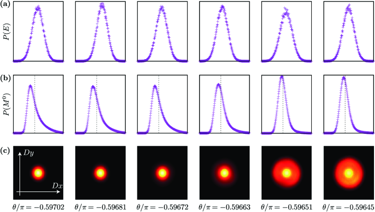
Figure 5: Histograms for energy (a), nematic along with a vertical line marking the mean (b) and VBC (c) for $L=32,\beta=2L$ and values of $\theta$ on either side of the phase transition.

Energy histograms — A first order phase transition can be detected, if strong enough, by the existence of two peaks in the histogram of energy (recorded during the Monte Carlo simulations) corresponding to energies of the two coexisting phases. In the top panel of Fig. 5, we present energy histograms for a system size $L=32$ for different values of $\theta$ close to and across the quantum phase transition, where we observe no sign of such double-peak feature.

Nematic order parameter distribution — For the SO$(6)$ version of the Hamiltonian, each site can take one of 6 colors. To study the nematic ordering we use a 6-dimensional nematic order parameter as defined in the main text. In the disordered phase, $M^{c}$ is expected to have a Gaussian distribution with mean zero and independent of all $M^{c^{\prime}\neq c}$. This implies that a Binder cumulant defined as $U_{M_{c}}=\frac{\braket{(M^{c})^{4}}}{\braket{(M^{c})^{2}}^{2}}$ evaluates to three in the disordered phase. In the ordered phase, $U_{M_{c}}$ evaluates to a finite value which is not unity due to the SO$(6)$ symmetry. This can be observed in the histograms of the nematic order parameter shown in Fig. 5 (middle panel), as crossing the quantum phase transition. The distribution changes from Gaussian in the VBC phase where the nematic order parameter is disordered (right side of the panels), to a skewed distribution whose shape is dictated by the underlying SO$(6)$ symmetry in the nematic phase (left side). Once again we find a lack of double-peak distributions, showing consistency with a continuous phase transition on length scale $L=32$.

To understand the shape of this distribution, consider first a sample product state drawn from the Monte Carlo simulation in the nematic ${{\mathbb{N}}}$ basis. Note that in this basis the nematic phase corresponds to a simple SO$(6)$ ferromagnet. Let us denote the fraction of sites hosting color ${{\mathbb{N}}}_{c}$ as $a_{c}$. As we expect nematic ordering, without loss of generality, $a_{0}$ can be assumed to be larger than all other $a_{c}$, and all other $a_{c}$ equal due to the remnant symmetry between the non-dominant colors. Now consider the operator $M^{0}_{i}=\ket{{{\mathbb{N}}}_{0}}\bra{{{\mathbb{N}}}_{0}}$ acting at site $i$. Using the shorthand $\ket{c}=\ket{{{\mathbb{N}}}_{c}}$ only for this section, we see that $\braket{c}{M^{0}_{i}}{c^{\prime}}=1$ for $c=c^{\prime}=0$ and 0 otherwise. As the product state of the system is representative of the ordering, we must include all states reached by SO$(6)$ rotations starting from this state. This can be engineered in a straightforward manner by applying the rotation on $M^{0}_{i}$ using an SO$(6)$ rotation matrix $O$ as $O^{T}M^{0}_{i}O$. Due to the constraints on $M^{0}_{i}$, this reduces to the matrix $A_{kl}=O_{0k}O_{0l}$. As we are working with a product state, applying this at site $i$ in state $c$, we get $\braket{A}_{i}=(O_{0c})^{2}$. As we have assumed that the fraction of sites in state $c$ is $a_{c}$, $\sum_{i}\braket{A}_{i}$ reduces to $\sum_{c}a_{c}(O_{0c})^{2}$. Using the conditions that all $a_{c}$ are equal except $a_{0}$ and $\sum_{c}a_{c}=1$, we can write $a_{0}=\frac{1}{6}+r$ and $a_{c\neq 0}=\frac{1}{6}-\frac{r}{5}$. This implies that $\sum_{c}a_{c}(O_{0c})^{2}$ can be broken into $(\frac{1}{6}-\frac{r}{5})\sum_{c}(O_{0c})^{2}+(r+\frac{r}{5})(O_{00})^{2}$. We can reduce the first term by using the identity $OO^{T}=I$, which implies $\sum_{c}O_{0c}O^{T}_{c0}=\sum_{c}O_{0c}O_{0c}=1$. This leaves a dependency on the SO$(6)$ matrix given only by $(O_{00})^{2}$, which must be averaged uniformly over all realizations of the rotation matrix. As $O_{00}$ is one component of a unit vector chosen at random in six-dimensional space, its distribution can be calculated analytically by considering a particular value of the first component. The probability of this value lying between $x$ and $x+dx$ is given by the volume of the five-dimensional shell over which the rest of the components are distributed. Using the expression for the surface area of a five-dimensional sphere, we can deduce that $p(x)\propto(1-x^{2})^{3/2}$.

We use the above arguments to calculate the theoretical prediction for the value of the Binder cumulant $U_{M_{c}}$ in the nematic phase. First, we note that $M^{0}$ for $U_{M_{0}}$ is defined to have a zero mean, i.e, $M^{0}=\sum_{i}(M_{i}^{0}-1/6)$. The relevant powers to be calculate for $U_{M_{0}}$ are $\braket{(M^{0})^{4}}$ and $\braket{(M^{0})^{2}}$. Let us first begin with the quadratic term. Expanded in the site index, this assumes the form $\sum_{i,j}(M_{i}^{0}-1/6)(M_{j}^{0}-1/6)$. Under an $SO(6)$ rotation, each term (denoted by $A_{ij}$ for convenience) in the sum transforms to $[O_{ak}(\delta_{a0}-1/6)O_{al}]_{i}[O_{bm}(\delta_{b0}-1/6)O_{bn}]_{j}$, where repeated indices are summed over and $[]_{a}$ indicates that the operator acts on site $a$. Now we can evaluate $A_{ij}$ in the product state where the state at site $i(j)$ is given by $c_{i(j)}$. This leads to $\braket{A_{ij}}=(O_{0c_{i}}^{2}-1/6)(O_{0c_{j}}^{2}-1/6)$. The double sum over all sites, $\sum_{ij}A_{ij}$, can now be written in a factorized form as $\sum_{c}a_{c}(O_{0c}^{2}-1/6)\sum_{d}a_{d}(O_{0d}^{2}-1/6)$. Each individual sum in this expression has already been evaluated to $(r+\frac{r}{5})(O_{00})^{2}-\frac{r}{5}$. Using the probability distribution of $x=O_{00}$ discussed in the paragraph above, we can now express $\braket{(M^{0})^{2}}$ as the integral $(1/N)\int_{-1}^{1}(6x^{2}-1)^{2}p(x)dx$, where $N$ is the normalization of the probability distribution, given by $\int_{-1}^{1}p(x)dx$. A similar analysis for the fourth power leads to $\braket{(M^{0})^{4}}=(1/N)\int_{-1}^{1}(6x^{2}-1)^{4}p(x)dx$. Combining these results, we can conclude that the value of Binder cumulant in a nematic ordered state is

$$U_{M_{0}}=\frac{\frac{1}{N}\int_{-1}^{1}(6x^{2}-1)^{4}p(x)dx}{\big{[}\frac{1}{N}\int_{-1}^{1}(6x^{2}-1)^{2}p(x)dx\big{]}^{2}}=\frac{114}{25}.$$ (12)

We find that the expectation $U_{M_{0}}=\frac{114}{25}=4.56$. is in agreement with the Monte Carlo simulations presented below in the region of parameter space where we expect nematic ordering.

VBC order parameter distribution — To detect VBC ordering, we use $D^{2}=D_{x}^{2}+D_{y}^{2}$ (with $D_{x}=\sum_{i}(-1)^{i_{x}}C_{i_{x},i_{y}}\cdot C_{i_{x}+1,i_{y}}$ and $D_{y}=\sum_{i}(-1)^{i_{y}}C_{i_{x},i_{y}}\cdot C_{i_{x},i_{y}+1}$ as in the main text) and similarly define the Binder cumulant as $U_{D}=\frac{\braket{(D^{2})^{2}}}{\braket{D^{2}}^{2}}$. In the disordered phase $(D_{x},D_{y})$ form a two-dimensional Gaussian distribution leading to $U_{D}=2$. In the ordered phase, $U_{D}=1$ as fluctuations in $D^{2}$ are small compared to its mean value. Note that $D^{2}$ is sensitive only to the development of non-zero VBC ordering and does not differentiate between various types of VBC orderings, such as columnar and plaquette.

The histograms for the VBC order parameter shown in the bottom panel of Fig. 5 all show a circular shape but with a finite radius that decreases as one moves towards the nematic phase (the finite value of the left panels located in the nematic phase are associated to the finite size $L=32$).

Binder cumulants — We finally present in Fig. 6 the values of Binder cumulants as a function of $\theta$ close the phase transition, for different system sizes. We observe a non-trivial non-monotonous behavior for both nematic $U_{M_{c}}$ (top panel), and VBC $U_{D}$ (bottom panel) Binder cumulants.

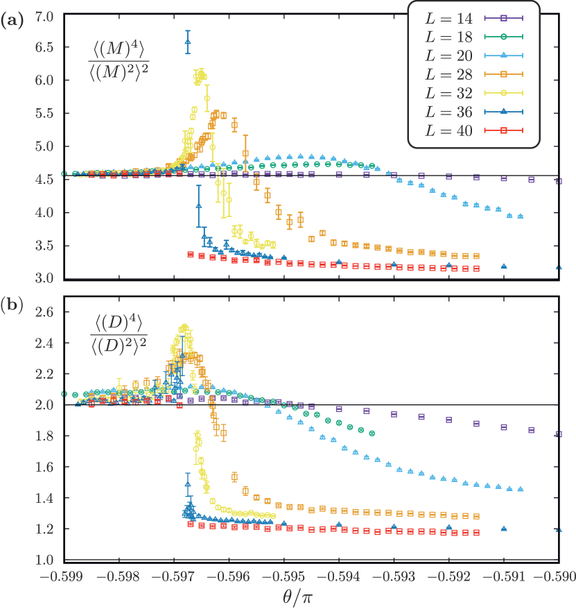
Figure 6: (a) Binder cumulant of the nematic order parameter and (b) the VBC order parameter showing a single critical point, and strong non-monotonic behavior.

For the nematic Binder cumulant, data on small systems range within the disordered value $3$ (reached for large enough $\theta$) and the expected ordered value $4.56$ (reached for $\theta<\theta_{c}$). On the other hand, starting from $L\simeq 18$, the Binder cumulant curve overshoots the ordered value as one approaches the transition point $\theta_{c}$ from above, with curves showing a steeper overshoot as $L$ is increased. For a first order transition, a somewhat similar behavior is predicted Vollmayr et al. (1993) on the basis of a two-peak distribution of the order parameter (which we do not observe, see above) resulting in a value of the Binder cumulant at the maximum scaling with volume $L^{2}$. We have checked that the maximum of $U_{M_{c}}$ does not scale as the volume $L^{2}$, at least on the lattice sizes accessible to us. Curves for different system sizes cross at different values of $\theta$, which is usually indicative of a first order transition (but note however the very narrow range of $\theta$ displayed in Fig. 6). The non-monotonous behavior does not allow to conclude on the order of the phase transition (in particular a data collapse is not satisfying), but we note that the sharp overshoot feature is converging towards our estimate of $\theta_{c}\simeq-0.5969\pi$ obtained from stiffness crossing (see main text).

A similar, albeit slightly different, non-monotonous behavior is observed for the VBC Binder cumulant, with a somewhat smoother overshoot over the disordered value of the Binder cumulant. Here again the maximum does not scale with volume, and could actually be converging to a finite value given the data on the largest systems that we could simulate ($L=36,40$). The maximum anomaly also converges towards our estimate of $\theta_{c}$.

Overall we conclude that the Binder cumulants of both order parameters do not display the behaviors expected either at a continuous phase transition (no clear unique crossing point) or at a (strong) first-order phase transition (with an anomaly scaling as the volume of the system size).

V Nature of the U($1$) symmetry in the VBC phase

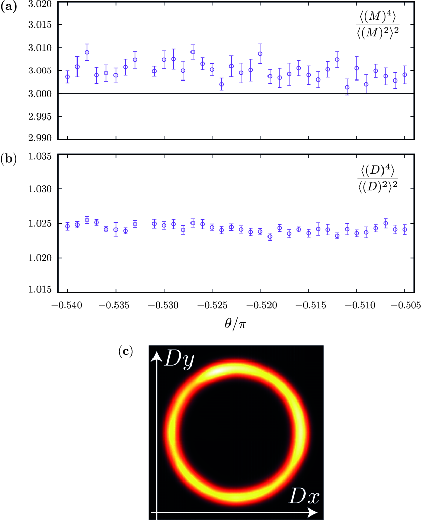
Figure 7: Binder cumulants for nematic (a) and VBC (b) order parameters for $L=96$ and $\beta=24$. (c) Heat map shows histogram for the VBC order parameter for $L=96,\theta=-0.52\pi,\beta=12$.

Here we show evidence for the nature of the VBC phase by studying a large $L=96$ lattice. In order to determine the nature of the phase, we display in the top panel of Fig. 7, the nematic Binder cumulant in the range $[-0.54\pi,-0.5\pi]$ and we clearly see that it approaches close to the expected value of $3$ in the disordered phase. On the other hand, the VBC Binder cumulant (middle panel is close to $1$) in the same range, as expected for an ordered VBC state.

Figure 8: (a) The negative second derivative of the ground state energy per site $-L^{-d}\frac{\partial^{2}E}{\partial(\cos\theta)^{2}}$ calculated using $\beta=2L$ shows a divergence close to the phase transition at $\theta=-0.596\pi$. (b) Scaling of the peak with system size on a log-log plot, fit to $aL^{b}$ yields $b=5.2(3)$.

This preliminary check being performed, we now seek for the specific symmetry breaking pattern of the VBC. We find that even at this large system size $L=96$, there is no obvious discrete symmetry breaking, as we report in the bottom panel of Fig. 7 for $\theta=-0.52\pi$. There the sample histogram of the VBC order parameter at a relatively low temperature of $\beta=12$ clearly displays a U($1$) symmetry. Note that we are unable to simulate lower temperatures for $L=96$ due to ergodicity constraints and finite statistics of our simulations, as the system is able to sample only a portion of, and not the full, circle. As seen for the Binder cumulant of the VBC order parameter in Fig. 6, this finite statistics issue does not affect the estimation of the magnitude fluctuations. Recalling that a component of $\vec{M}$ is defined as $M^{s}=\frac{1}{N}(\sum_{i}\ket{{{\mathbb{N}}}_{s}}\bra{{{\mathbb{N}}}_{s}})-\frac{1}{6}$, we see that $\langle(M^{s})^{2}\rangle$ yields a non-zero value for nematic ordering.

VI 2nd derivative of energy

The second derivative of the ground state energy per unit site w.r.t $\cos(\theta)$ can be calculated using the formalism developed in Ref. Albuquerque et al. (2010), where the Hamiltonian is of the form $H_{0}+gH_{1}$, and the derivative is calculated w.r.t $g$. Since our Hamiltonian is of the form $\alpha H_{1}+\gamma H_{2}$ with $\alpha=\cos\theta$ and $\gamma=\sin\theta-\cos\theta$, we have to consider the derivative for both terms and the expression reduces to

$$-\frac{\partial^{2}E}{\partial(\cos\theta)^{2}}=\frac{1}{\beta}\bigg{[}\frac{A_{1}}{\alpha^{2}}+\bigg{(}\frac{1}{\gamma}\frac{\partial^{2}\gamma}{\partial\alpha^{2}}+\frac{1}{\gamma^{2}}\bigg{(}\frac{\partial\gamma}{\partial\alpha}\bigg{)}^{2}\bigg{)}A_{2}\\ +\bigg{(}\frac{2}{\alpha\gamma}\frac{\partial\gamma}{\partial\alpha}+\frac{1}{\gamma}\frac{\partial^{2}\gamma}{\partial\alpha^{2}}\bigg{)}A_{12}\bigg{]}$$

with

$$A_{1}=\langle N_{1}^{2}\rangle-\langle N_{1}\rangle-\langle N_{1}\rangle^{2},$$

$$A_{2}=\langle N_{2}^{2}\rangle-\langle N_{2}\rangle-\langle N_{2}\rangle^{2},$$

$$A_{12}=\langle N_{1}N_{2}\rangle-\langle N_{1}\rangle\langle N_{2}\rangle.$$

where $N_{1(2)}$ corresponds to the number of operators of type $H^{1(2)}$ in an operator string generated by the stochastic series expansion and $\langle\ldots\rangle$ the standard Monte Carlo average.

The negative second derivative estimated using the expression above is displayed around the expected phase transition in the top panel of Fig. 8. We observe that it diverges with system size, with a maximum approaching the critical point.

At a continuous quantum phase transition in dimension $d$, the second derivative of the energy is expected to scale as $-L^{d}\frac{\partial^{2}E}{\partial(\cos(\theta))^{2}}\propto L^{2/\nu-(d+z)}$ where $\nu$ is the correlation length exponent and $z$ the dynamical critical exponent Albuquerque et al. (2010). Assuming a continuous phase transition takes place and that $z=1$ (see scaling of the stiffness in the main text), a fit of the divergence of the peak (shown in the bottom panel of Fig. 8) leads to an exponent $1/\nu=4.1(2)$, which is anomalously quite large.

We conclude that while a divergence of the second derivative of the energy is compatible within system sizes $L\leq 32$ with a continuous transition, the anomalously large value of the effective correlation length exponent that we obtain $1/\nu=4.1(2)$ hints towards a first-order character of the phase transition, which is confirmed by the time trace presented for larger system size in the main manuscript.

VII Comparison with SO(5) nematic to VBC transition

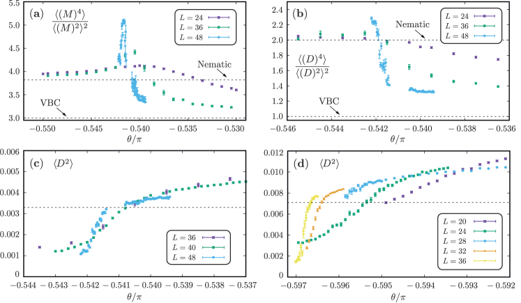
Figure 9: Binder cumulants for nematic (a) and VBC (b) order parameters for $SO(5)$ symmetric microscopic degrees of freedom as a function of $\theta/\pi$, where constant lines mark the expected values in the two phases. (c) and (d) show the expectation value of the VBC order parameter for $SO(5)$ and $SO(6)$ respectively. A crossing point is visible with increasing system size, and a rough estimate of the thermodynamic value of the discontinuity in the order parameter is given by dashed constant lines.

To understand the change in the nature of the transition with changing number of components accessible to the microscopic nematic degree of freedom, we simulate the nematic Hamiltonian (Eq. (10)) for 5 possible colors on each site. These simulations are motivated by the relevance of SO(5) symmetry for e.g. spin-3/2 fermionic cold atom systems Wu et al. (2003); Wu (2006).

In the phase space region defined by $\theta/\pi\in(-0.75,-0.5)$, we find a nematic and VBC phase, separated by a direct transition, similar to the $SO(6)$ case studied in the main text. The behavior of both Binder cumulants is shown as a function of $\theta/\pi$ in Figs. 9 (a) and (b).

To identify the nematic phase, we calculate the Binder cumulant of the nematic order parameter defined similarly as in the $SO(6)$ case. Repeating the argument above for the case of an $SO(5)$ symmetry, we find $p(x)\propto(1-x^{2})$ for the distribution of the first component and that the Binder cumulant is re-expressed as $\displaystyle U_{M_{0}}=\frac{\frac{1}{N}\int_{-1}^{1}(5x^{2}-1)^{4}p(x)dx}{\big{[}\frac{1}{N}\int_{-1}^{1}(5x^{2}-1)^{2}p(x)dx\big{]}^{2}}=\frac{42}{11}$.

We find (Fig. 9 (a)) that the nematic Binder cumulant tends to the predicted theoretical value $42/11\simeq 3.818$ in the parameter range $\theta/\pi\in(-0.75,-0.5443(2))$, beyond which we find a VBC phase, indicated by the approach of the VBC Binder Cumulant to unity (Fig. 9 (b)) We also observe the development of a non-monotonic behavior with increasing size similar to the $SO(6)$ case, indicating a possible first order transition.

While it is difficult to differentiate between weak and very weak first order phase transitions given the large scale lengths involved and the large number of components in these models, we now present two numerical observations which lead us to conclude that the first order nature for $SO(5)$ is weaker than the same for $SO(6)$.

The first of this is the ergodicity achieved by our QMC algorithm for sizes close to $L=48$ for $SO(5)$. As we have shown in the main text, the algorithm suffers from strong metastability for a size of $L=40$ for $SO(6)$, making it impossible for us to get reliable data for larger sizes. This feature is absent for $SO(5)$ at least till sizes of $L=72$. This shows that the transition is not of a strong first order nature, where we would expect the algorithm to oscillate between two qualitatively different phases.

The second observation involves the behavior of the VBC order parameter close to the transition as it approaches zero. Both $SO(5)$ (Figs. 9 (c)) and $SO(6)$ (Figs. 9 (d)) show crossing points in the VBC order parameter, which are not expected at a conventional continuous transition. This allows us to estimate the size of the discontinuity in the VBC order parameter at the transition (assuming that it is first order) and we show a rough estimation of the thermodynamic discontinuity in both plots using dashed constant lines. A comparison of Figs. 9 (c) and (d) shows that the discontinuity for $SO(6)$ is roughly a factor of 2 greater than that for $SO(5)$, also suggesting that the $SO(5)$ symmetry realises a weaker first order transition.