Nyquist Sampling and Degrees of Freedom
of Electromagnetic Fields

Abstract

A signal space approach is presented to study the Nyquist sampling, number of degrees of freedom and reconstruction of an electromagnetic field under arbitrary scattering conditions. Conventional signal processing tools, such as the multidimensional sampling theorem and Fourier theory, are used to provide a linear system theoretic interpretation of electromagnetic wave propagation, thereby revealing the spatially bandlimited nature of electromagnetic fields. Their spatial bandwidth is dictated by the selectivity of the underlying scattering that allows establishing the Nyquist spatial sampling with a reduction of the number of fields’ samples needed to be processed.

I Introduction

The Kotelnikov-Shannon-Whittaker sampling theorem [2, 3, 4] states that any squared-integrable signal of finite bandwidth $\Omega/\pi$ Hz, ${e(t)\in\mathcal{B}_{\Omega}}$ for $t\in\mathbb{R}$, can be perfectly reconstructed from its samples taken at equally spaced ${Q^{\star}=\pi/\Omega}$ seconds apart by the reconstruction formula (also called cardinal series)

$$e(t)=\sum_{n\in\mathbb{Z}}e\left(nQ^{\star}\right)f_{\Omega}\left(t-nQ^{\star}\right)$$ (1)

where $f_{\Omega}(t)=\mathrm{sinc}\left(t/Q^{\star}\right)$. Orthonormality is a fundamental property of the reconstruction sinc-functions, which allows to geometrically interpret the samples as coordinates of a basis set of functions [2]. In general, $e(t)$ may not be bandlimited, and an ideal low-pass filtering operation is required prior to sampling with reduced reconstruction accuracy [5].

The generalization of the sampling theorem in (1) to spatially bandlimited fields is known as multidimensional sampling theorem [6, 7, 8, 9]. With respect to the classical definition of a bandlimited signal in the frequency domain, this notion applies in the spatial-frequency (wavenumber) domain [10, Ch. 8]. Its application requires an accurate description of the field in the spectral domain, which is tied to its physical nature. For wireless researchers, the class of three-dimensional (3D) electromagnetic fields is of great interest as they allow transfer of information from one point to another [11]. A field of this sort generates a continuum of spatial samples in the form of an analog physical process. Yet the noise allows for a certain error in the field description, calling for a discrete representation through spatial sampling.

In processing analog fields, it is highly desirable to minimize the sampling rate because the amount of data processing, power consumption, and digital storage is proportional to the number of samples to be processed [12]. This is of paramount importance at high frequencies (e.g., millimeter wave and sub-terahertz spectrum) where the complex nature of propagation channels requires to collect a large amount of measurements [13].

Motivated by the above considerations, this paper revisits the sampling theory for electromagnetic fields with potential applications to, e.g., channel sounding, sensing and localization at high frequencies. We deviate from the electromagnetic literature [14, 15], and provide a signal processing interpretation of wave propagation under arbitrary scattering conditions. Precisely, 3D wireless propagation can be modeled as a two-dimensional (2D) linear and space-invariant (LSI) system with low-pass filtering behavior. Physics-driven approaches similar to the one used in this paper can be found in [16, 17, 18], where the number of degrees of freedom (DoF) that can be extracted from electromagnetic fields, confined in a space region with spherical symmetry, is computed.

Unlike [16, 17, 18], we consider regions of rectangular symmetry and perform the analysis in Cartesian coordinates, by leveraging the connection with Fourier theory [19, 20, 21, 22, 23]. In addition, we connect the DoF result with the Nyquist sampling and field reconstruction problem. Notice that asymptotic results such as DoF and sampling theorem become more accurate as the wavelength shortens (i.e., high frequencies). Both were studied in [24] under isotropic scattering.

We generalize [24] to an arbitrary configuration of scatterers and provide an alternative explanation of the results via a signal processing approach. The development is finally extended to ensembles of stationary electromagnetic Gaussian random fields [20, 21, 22, 23].

I-A Outline of the Paper

The remainder of this paper is organized as follows. In Section II, we review the sampling theorem and put much emphasis on the interplay among Nyquist sampling, reconstruction, and number of DoF. In Section III, we provide a spectral characterization of the class of 3D electromagnetic fields. This is first used in Section IV to solve the Nyquist sampling and reconstruction problem and later in Section V to compute the DoF. The generalization of the developed framework to ensembles of stationary electromagnetic random fields is provided in Section VI. Numerical results are given in Section VII to validate the developed theory under practical settings. Conclusions are drawn in Section VIII.

I-B Notation

We use upper (lower) case letters for spatial-frequency (spatial) entities. Boldfaced letters indicate vectors and matrices. The superscripts ${}^{\mbox{\tiny$\mathrm{T}$}}$, ^-1, and ^1/2 stand for transposition, inverse, and matrix square root, respectively. $\mathrm{diag}(\mathbf{x})$ indicates the diagonal matrix with elements from $\mathbf{x}$. $\det(\mathbf{X})$ is the determinant of $\mathbf{X}$. $\mathbf{I}_{n}$ is the $n$-dimensional identity matrix. Calligraphic letters indicate sets. $m(\mathcal{X})$ denotes the Lebesgue measure, $\mathbbm{1}_{\mathcal{X}}(x)$ is the indicator function. $\mathbb{R}^{n}$ and $\mathbb{Z}^{n}$ are the $n$-dimensional spaces of real-valued and integer numbers, $|\cdot|$ denotes absolute value, $\lceil x\rceil$ denotes the least integer greater than or equal to $x$, $\mathrm{sinc}(x)=\sin(\pi x)/(\pi x)$ is the sinc function, $\mathrm{jinc}(x)=J_{1}(x)/x$ is the jinc function where $J_{1}(x)$ denotes the Bessel function of the first kind with order $1$. A general point $(\mathbf{r},z)\in\mathbb{R}^{3}$ is described by its Cartesian coordinates $(x,y,z)$ with $\|\mathbf{r}\|=\sqrt{x^{2}+y^{2}+z^{2}}$ the Euclidean norm. $\nabla^{2}=\frac{\partial^{2}}{\partial x^{2}}+\frac{\partial^{2}}{\partial y^{2}}+\frac{\partial^{2}}{\partial z^{2}}$ is the Laplacian operator. $\mathbb{E}\{\cdot\}$ denotes the expectation operator. The notation $n\sim\mathcal{N}_{\mathbb{C}}(0,\sigma^{2})$ stands for a circularly symmetric complex Gaussian random variable with variance $\sigma^{2}$.

II Preliminaries

To make the paper self-contained, we briefly review the sampling theorem in one and two dimensions. This is preparatory for studying spatial electromagnetic fields.

II-A Time-domain Signals

Let $e(t)$ be a baseband signal with its spectrum ${E}(\omega)$. Uniform sampling of $e(t)$ at equally spaced $Q$ seconds apart yields the sampled signal ${e}_{\rm s}(t)=\sum_{n\in\mathbb{Z}}{e}(nQ)\delta(t-nQ)$ with spectrum [6, Sec. 3]

$$E_{\rm s}(\omega) =\sum_{n\in\mathbb{Z}}{e}(nQ)e^{-\mathsf{j}\omega nQ}$$ (2)

$$=\frac{1}{Q}\sum_{\ell\in\mathbb{Z}}{E}(\omega-\ell P)$$ (3)

where the frequency replication period $P$ is such that

$$PQ=2\pi.$$ (4)

For any bandlimited signal $e(t)\in\mathcal{B}_{\Omega}$ of bandwidth $\Omega/\pi$ (in Hz), the Nyquist sampling interval

$$Q^{\star}=\pi/\Omega$$ (5)

provides the minimum number of samples per unit of time (i.e., the Nyquist rate ${\mu=1/Q^{\star}}$ (in samples/s)) that is needed for perfect reconstruction of $e(t)$ from its samples $\{{e}(nQ)\}$. Precisely, under Nyquist sampling, $E(\omega)$ can be perfectly retrieved by low-pass filtering the fundamental replica of $E_{\rm s}(\omega)$ in (3) with no aliasing,

$$E(\omega)=E_{\rm s}(\omega)\left(Q^{\star}\mathbbm{1}_{|\omega|\leq\Omega}(\omega)\right).$$ (6)

The reconstruction formula in (1) for $e(t)$ at any $t\in(-\infty,\infty)$ is obtained by an inverse Fourier transform of (6) with $E_{\rm s}(\omega)$ given by (2) [6, Sec. 3], [2]. The interpolating sinc-function does not depend on the spectral characteristics of $E(\omega)$, but only on the measure of its support, i.e., the bandwidth $\Omega$.

Given the continuous nature of $e(t)$, signals belonging to $\mathcal{B}_{\Omega}$ span an infinite-dimensional space. However, noise and quantization effects allows a certain error in the representation so that bandlimited signals are amenable to a representation over a set of approximately DoF dimension [10, Sec. 2]. Within a time interval of duration $T$, since there are $1/Q^{\star}$ samples/s, we have a total of [10, Eq. (2.14)]

$$\mathrm{dof}_{[-\Omega,\Omega]}=\frac{\Omega T}{\pi}$$ (7)

significant samples in the interval. The implication of (7) is that only a finite number of samples carries the essential information contained in the signal and can be used to reconstruct it. The reconstruction error decreases as $\Omega T$ increases and vanishes at infinity [10, Sec. 2]. Sampling above the Nyquist rate does not create any additional DoF and adds an insignificant contribution to the signal’s reconstruction.

II-B 2D Spatial Fields

The generalization of a 1D uniform sampling to a 2D lattice $\mathbf{Q}\mathbf{n}$ given $\mathbf{Q}\in\mathbb{R}^{2\times 2}$ the (non-singular) sampling matrix yields ${e}_{\rm s}(\mathbf{r})=\sum_{\mathbf{n}\in\mathbb{Z}^{2}}{e}(\mathbf{Q}\mathbf{n})\delta(\mathbf{r}-\mathbf{Q}\mathbf{n})$ [6, Sec. 6]. As an example, a simple 2D rectangular sampling is obtained when $\mathbf{Q}=\mathrm{diag}(q_{x},q_{y})$ where $q_{x}$ and $q_{y}$ are the sampling intervals along the $x-$ and $y$-axis, respectively. The spatial Fourier transform of ${e}_{\rm s}(\mathbf{r})$ is [6, Sec. 6]

$$E_{\rm s}(\mathbf{k}) =\sum_{\mathbf{n}\in\mathbb{Z}^{2}}{e}(\mathbf{Q}\mathbf{n})e^{-\mathsf{j}\mathbf{k}^{\mbox{\tiny$\mathrm{T}$}}\left(\mathbf{Q}\mathbf{n}\right)}$$ (8)

$$=\frac{1}{|\det(\mathbf{Q})|}\sum_{\boldsymbol{\ell}\in\mathbb{Z}^{2}}{E}\left(\mathbf{k}-\mathbf{P}\boldsymbol{\ell}\right)$$ (9)

where the periodicity matrix $\mathbf{P}\in\mathbb{R}^{2\times 2}$ is related to $\mathbf{Q}$ as

$$\mathbf{P}^{\mbox{\tiny$\mathrm{T}$}}\mathbf{Q}=2\pi\mathbf{I}_{2}.$$ (10)

For any bandlimited field $e(\mathbf{r})\in\mathcal{B}_{\mathcal{K}}$ of spatial bandwidth $m(\mathcal{K})$ (in (rad/s)²), we denotes with $\mathbf{P}^{\star}$ the Nyquist periodicity matrix that provides the minimum interspacing among adjacent replicas of ${E}(\mathbf{k})$ with no overlapping. The associated Nyquist sampling matrix

$$\mathbf{Q}^{\star}=2\pi(({\mathbf{P}^{\star}})^{\mbox{\tiny$\mathrm{T}$}})^{-1}$$ (11)

provides the minimum number of samples per unit of space, i.e., the Nyquist density (in samples/m²) [7, 25]

$$\mu=\frac{1}{|\det(\mathbf{Q}^{\star})|}$$ (12)

that is needed for perfect reconstruction of $e(\mathbf{r})$ from its samples $\{{e}(\mathbf{Q}^{\star}\mathbf{n})\}$. This extends the notion of Nyquist sampling rate (in samples/m) to spatial fields. As in (6), under Nyquist sampling, $E(\mathbf{k})$ can be perfectly retrieved by low-pass filtering $E_{\rm s}(\mathbf{k})$,

$$E(\mathbf{k})=E_{\rm s}(\mathbf{k})\left(|\det(\mathbf{Q}^{\star})|\mathbbm{1}_{\mathcal{K}}(\mathbf{k})\right).$$ (13)

The 2D counterpart of (1) is obtained via an inverse Fourier transform of (13) with $E_{\rm s}(\mathbf{k})$ in (8) [6, Eq. (6.33)]:

$$e(\mathbf{r})=\sum_{\mathbf{n}\in\mathbb{Z}^{2}}e(\mathbf{Q}^{\star}\mathbf{n})f_{\mathcal{K}}(\mathbf{r}-\mathbf{Q}^{\star}\mathbf{n})$$ (14)

with interpolating function [6, Eq. (6.34)]

$$f_{\mathcal{K}}(\mathbf{r}) =\frac{|\det(\mathbf{Q}^{\star})|}{(2\pi)^{2}}\int_{\mathbb{R}^{2}}\mathbbm{1}_{\mathcal{K}}(\mathbf{k})e^{\mathsf{j}\mathbf{k}^{\mbox{\tiny$\mathrm{T}$}}\mathbf{r}}\,d\mathbf{k}.$$ (15)

Similarly to the 1D case, Nyquist sampling and interpolating function do not depend on the values assumed by $E(\mathbf{k})$, but solely by the shape of its support $\mathcal{K}$. Unfortunately, these cannot be computed univocally from its measure (as for 1D signals) as multidimensional supports are described by more than one parameter [8]. Our focus is on 3D scalar electromagnetic fields generated by arbitrary scattering conditions. A scalar formulation physically corresponds to acoustic wave propagation in general [18, 26] or electromagnetic wave propagation in a source-free environment [27]. Their spectral support is characterized next.

III Spectral Characterization of Electromagnetic Fields

The generalization of sampling theorem to multiple dimensions requires a spectral characterization of the considered field. This is addressed next for electromagnetic fields, generated by the interaction of a radiated field with an arbitrary configuration of scatterers in the half-space $\{z<0\}$. Upon interaction, a scattered field propagating in a 3D homogeneous and isotropic medium is measured at receiver, modeling a non line-of-sight propagation scenario. Under these settings, the Maxwell’s equations reduce to the vector (source-free) homogeneous Helmholtz equations [27, Eq. (1.2.20)]

$$\left(\nabla^{2}+\frac{\partial^{2}}{\partial z^{2}}\right)\mathbf{e}(\mathbf{r},z)+\kappa^{2}\mathbf{e}(\mathbf{r},z)=0$$ (16)

where $\mathbf{e}(\mathbf{r},z)$ with ${\mathbf{r}=(x,y)\in\mathbb{R}^{2}}$ can be either the electric or magnetic vector fields and $\kappa=2\pi/\lambda$ is the wavenumber with $\lambda$ the wavelength. We do our analysis in Cartesian coordinates, i.e., $\mathbf{e}(\mathbf{r},z)=\hat{\mathbf{x}}e_{x}+\hat{\mathbf{y}}e_{y}+\hat{\mathbf{z}}e_{z}$. In this case, (16) can be addressed independently along each coordinate [28]. In a line-of-sight scenario, the capability of an observer to resolve features of the radiated field is distance-dependent. This effect should be accounted for by considering an inhomogeneous equation driven by the distribution of the radiator [29].

III-A Scalar Homogeneous Helmholtz Equation

\begin{overpic}[width=260.17464pt,tics=10]{Fig1} \end{overpic}

Figure 1: Wave propagation in a 3D homogeneous, isotropic, and source-free medium can be modeled as a low-pass filter.

Without loss of generality, we denote with $e(\mathbf{r},z)$ either $e_{x}$, $e_{y}$ or $e_{z}$. This field obeys the scalar homogeneous Helmholtz equation [27, Eq. (1.2.21)]

$$\left(\nabla^{2}+\frac{\partial^{2}}{\partial z^{2}}\right)e(\mathbf{r},z)+\kappa^{2}e(\mathbf{r},z)=0$$ (17)

or in the horizontal spatial-frequency (wavenumber) domain,

$$\frac{\partial^{2}}{\partial z^{2}}E(\mathbf{k},z)+(\kappa^{2}-\|\mathbf{k}\|^{2})E(\mathbf{k},z)=0$$ (18)

where ${\mathbf{k}=(k_{x},k_{y})\in\mathbb{R}^{2}}$ are the horizontal wavenumber Cartesian coordinates and

$$E(\mathbf{k},z)=\int_{\mathbb{R}^{2}}e(\mathbf{r},z)e^{-\mathsf{j}\mathbf{k}^{\mbox{\tiny$\mathrm{T}$}}\mathbf{r}}\,d\mathbf{r}.$$ (19)

For any fixed $\mathbf{k}\in\mathbb{R}^{2}$, (18) is a second-order ordinary differential equation in $z$ with constant coefficients whose general solution in the half-space $\{z\geq 0\}$ is of the form

$$E(\mathbf{k},z)=E(\mathbf{k})e^{\mathsf{j}k_{z}(\mathbf{k})z},$$ (20)

where $E(\mathbf{k})$ is an arbitrary complex-valued coefficient and $k_{z}(\mathbf{k})$ is defined as

$$k_{z}(\mathbf{k})=\begin{cases}\sqrt{\kappa^{2}-\|\mathbf{k}\|^{2}}&\mathbf{k}\in\mathcal{D}\\ \mathsf{j}\sqrt{\|\mathbf{k}\|^{2}-\kappa^{2}}&\text{elsewhere}\end{cases}$$ (21)

given

$$\mathcal{D}=\{\mathbf{k}\in\mathbb{R}^{2}:\|\mathbf{k}\|^{2}\leq\kappa^{2}\}$$ (22)

as a disk of radius $\kappa$; see Fig. 1. Notice that $\mathbf{k}$ can vary independently in $\mathbb{R}^{2}$ and hence $k_{z}(\mathbf{k})$ in (21) can be either real- or imaginary-valued with positive imaginary part. Particularly, $k_{z}(\mathbf{k})$ is real-valued within $\mathbf{k}\in\mathcal{D}$ and imaginary-valued otherwise. The spatial field $e(\mathbf{r},z)$ with $\{z\geq 0\}$ obeying (17) is obtained via a 2D inverse spatial Fourier transform of (20):

$$e(\mathbf{r},z)=\frac{1}{(2\pi)^{2}}\int_{\mathbb{R}^{2}}E(\mathbf{k})e^{\mathsf{j}k_{z}(\mathbf{k})z}e^{\mathsf{j}\mathbf{k}^{\mbox{\tiny$\mathrm{T}$}}\mathbf{r}}\,d\mathbf{k}.$$ (23)

III-B System-Theoretic Interpretation of Wave Propagation

\begin{overpic}[width=390.25534pt,tics=10]{Fig2a} \end{overpic}

(a) $z/\lambda=1$.

\begin{overpic}[width=390.25534pt,tics=10]{Fig2b} \end{overpic}

(b) $z/\lambda=10$.

Figure 2: Magnitude (in dB) of $H_{z}(\mathbf{k})$ in (24) for different $z$.

The spectrum-wise multiplication in (20) reveals that $e(\mathbf{r},z)$ with $\{z\geq 0\}$ can be obtained by passing a 2D field $e(\mathbf{r},0)$ with spectrum $E(\mathbf{k})$ through an LSI system (see Fig. 1) with wavenumber response

$$H_{z}(\mathbf{k})=e^{\mathsf{j}k_{z}(\mathbf{k})z}.$$ (24)

This operation is known in physics as migration (e.g., [7, Sec. 7]), and it is a direct consequence of the Helmholtz equation in (17), which acts as an LSI operator projecting the number of observable 3D field configurations onto a lower-dimensional 2D space [30]. Depending on $\mathbf{k}$, $H_{z}(\mathbf{k})$ in (24) is either an oscillatory or an exponentially-decaying function of ${z}$, i.e.,

$$H_{z}(\mathbf{k})=\begin{cases}e^{\mathsf{j}\sqrt{\kappa^{2}-\|\mathbf{k}\|^{2}}\,z}&\mathbf{k}\in\mathcal{D}\\ e^{-\sqrt{\|\mathbf{k}\|^{2}-\kappa^{2}}\,z}&\text{elsewhere}.\end{cases}$$ (25)

In the case $\mathbf{k}\in\mathcal{D}$, $H_{z}(\mathbf{k})$ is an all-pass filter that simply introduces a phase-shift along $z$. This implies that $e(\mathbf{r},z)$, at any $z$-plane is fully determined by $e(\mathbf{r},0)$. Outside of this support, $H_{z}(\mathbf{k})$ introduces an attenuation with exponential pace along $z$. This is quantified in Fig. 2 where the magnitude of $H_{z}(\mathbf{k})$ is plotted (in dB) for $z/\lambda=\{1,10\}$. At $z=10\,\lambda$, the field outside of $\mathcal{D}$ is attenuated more than $60$ dB. This means that, for distances $z$ larger than tens of wavelengths (i.e., for any practical distance from scatterers), we may consider $H_{z}(\mathbf{k})$ as a low-pass filter with maximum circular bandwidth

$$m(\mathcal{D})=\pi\kappa^{2}$$ (26)

which increases proportionally with the squared value of the operating frequency. This will be assumed in the remainder.

III-C Plane-Wave Decomposition

The integral in (23) has an intuitive physical interpretation in terms of a plane-wave decomposition of $e(\mathbf{r},z)$ where each plane wave impinges on the point $(\mathbf{r},z)$ from direction $(\mathbf{k}/\kappa,k_{z}(\mathbf{k})/\kappa)$ and has complex-valued amplitude $E(\mathbf{k})$ [21]. There are two types of plane waves in nature: the discarded evanescent waves and the remaining propagating waves. Hence, the field $e(\mathbf{r},z)$ in (23) can be approximated as

$$e(\mathbf{r},z) =\int_{\mathcal{D}}E(\mathbf{k})e^{\mathsf{j}(\mathbf{k}^{\mbox{\tiny$\mathrm{T}$}}\mathbf{r}+k_{z}(\mathbf{k})z)}\,d\mathbf{k}.$$ (27)

An equivalent representation of (27) can be obtained in the angular domain via cosine directions, which can be related to elevation $\theta\in[0,\pi/2]$ and azimuth $\phi\in[0,2\pi)$ angles as

$$\begin{pmatrix}\mathbf{k}\\ k_{z}(\mathbf{k})\end{pmatrix}=\begin{pmatrix}\kappa\sin(\theta)\cos(\phi)\\ \kappa\sin(\theta)\sin(\phi)\\ \kappa\cos(\theta)\end{pmatrix}.$$ (28)

Being interested in leveraging linear system theory and Fourier theory, we will privilege the wavenumber interpretation. The angular domain representation will be used in Section VI to characterize the angular selectivity of the scattering.

IV Nyquist Sampling and Reconstruction

Let us observe $e(\mathbf{r},z)$ over an infinite $z$-oriented plane and drop the functional dependance on $z$, i.e., ${e(\mathbf{r},z)=e(\mathbf{r})}$, as the sole effect introduced along the $z$-axis is the low-pass filtering operation introduced by migration. Reconstruction of the field at different $z$ requires compensating for the phase delay accumulated by the field along its travel along the $z$-axis. Differently from 3D reconstruction of an object, electromagnetic fields require to capture a single (not multiple) “image” of the field, which rests on the Huygen’s electromagnetic principle [27]. We consider scattering generated from a deterministic configuration of scatterers. Propagation into random media is treated in Section VI.

IV-A Half-wavelength Rectangular Sampling

The classical half-wavelength rectangular sampling arises as the Nyquist sampling for a spectrum with wavenumber support

$$\mathcal{R}=\{\mathbf{k}=(k_{x},k_{y})\in\mathbb{R}^{2}:|k_{x}|\leq\kappa,|k_{y}|\leq\kappa\}.$$ (29)

The problem of finding the Nyquist periodicity matrix $\mathbf{P}^{\star}_{\mathcal{R}}$ that yields the minimum separation among replicas is geometrically formulated as the arrangement of squares of sizes $2\kappa$ that achieves the highest density. Due to the rectangular symmetry of $\mathcal{R}$ in (29), this is solved, e.g., along the $k_{x}$-axis. The Nyquist sampling interval follows from (5) as $Q^{\star}_{x}={\pi}/{\kappa}=\lambda/2$ while using ${\kappa=2\pi/\lambda}$. Exchanging the $k_{x}$ and $k_{y}$ axes and rearranging the results into a matrix form yields [28]

$$\mathbf{Q}^{\star}_{\mathcal{R}}=\frac{\lambda}{2}\,\mathbf{I}_{2}.$$ (30)

The Nyquist density corresponding to (30) is given by

$$\mu_{\mathcal{R}}=\frac{1}{|\det(\mathbf{Q}^{\star}_{\mathcal{R}})|}=\frac{4}{\lambda^{2}}$$ (31)

The interpolating function for the reconstruction of $e(\mathbf{r})\in\mathcal{B}_{\mathcal{R}}$ is obtained from its 1D counterpart $f_{\Omega}(t)=\mathrm{sinc}\left(\Omega t/\pi\right)$ while replacing $\Omega$ with $\kappa=2\pi/\lambda$ and leveraging separability

$$f_{\mathcal{R}}(\mathbf{r})=\mathrm{sinc}\left(\frac{2x}{\lambda}\right)\mathrm{sinc}\left(\frac{2y}{\lambda}\right).$$ (32)

Based on the physical discussion in Section III-C, half-wavelength sampling involves a portion of evanescent waves into the analysis, which occurs only when the observation plane is located in the close proximity of the scatterers (see Fig. 2). For any practical scenario, it leads to an underutilization of the wavenumber spectrum with consequent loss of efficiency. We will develop on this observation later on.

IV-B Isotropic Scattering Environments

\begin{overpic}[width=346.89731pt,tics=10]{Fig3a} \end{overpic}

(a) Circle packing in the wavenumber domain.

\begin{overpic}[width=281.85034pt,tics=10]{Fig3b} \end{overpic}

(b) Hexagonal sampling in the spatial domain.

Figure 3: Nyquist sampling under isotropic scattering.

If no directionality is enforced by the scatterers, $e(\mathbf{r})\in\mathcal{B}_{\mathcal{D}}$. This case physically corresponds to an isotropic scattering environment where plane waves carry equal power from all possible directions ${\theta\in[0,\pi/2]}$ and ${\phi\in[0,2\pi)}$ [21, 20]. Hence, the problem of finding the Nyquist periodicity matrix $\mathbf{P}^{\star}_{\mathcal{D}}$ is geometrically found by solving a packing problem of circles of equal radius $\kappa$ [7, Sec. 1.4]. The solution is illustrated in Fig. 3(a) and obtained by first inscribing each circle with a regular hexagon of side lengths ${2\kappa}/{\sqrt{3}}$ (red line) and, then, replicating this hexagonal arrangement periodically such that no aliasing occurs [7, Eq. (1.148)]

$$\mathbf{P}^{\star}_{\mathcal{D}} =\begin{pmatrix}\sqrt{3}\kappa&\sqrt{3}\kappa\\ \kappa&-\kappa\end{pmatrix}.$$ (33)

Plugging (33) into (11) as in [7, Eq. (1.153)] while substituting $\kappa=2\pi/\lambda$ yields

$$\mathbf{Q}^{\star}_{\mathcal{D}} =\begin{pmatrix}\frac{\pi}{\kappa\sqrt{3}}&\frac{\pi}{\kappa\sqrt{3}}\\ \frac{\pi}{\kappa}&-\frac{\pi}{\kappa}\end{pmatrix}=\begin{pmatrix}\frac{\lambda}{2\sqrt{3}}&\frac{\lambda}{2\sqrt{3}}\\ \frac{\lambda}{2}&-\frac{\lambda}{2}\end{pmatrix}$$ (34)

and it corresponds to a hexagonal sampling, as illustrated in Fig. 3(b). The Nyquist density follows from (12) as

$$\mu_{\mathcal{D}}=\frac{1}{|\det(\mathbf{Q}^{\star}_{\mathcal{D}})|}=\frac{2\sqrt{3}}{\lambda^{2}}.$$ (35)

Notice that $\mathbf{Q}^{\star}_{\mathcal{D}}$ is not unique as there exist other sampling matrices all achieving the same efficiency [8, 9], e.g., by rotating the wavenumber axes by $\pi/2$. Compared to the half-wavelength rectangular sampling, we notice that $\mathcal{R}$ in (29) corresponds to the minimum squared embedding of $\mathcal{D}$. In turn, a hexagonal sampling has a sampling efficiency gain of

$$1-\frac{\mu_{\mathcal{D}}}{\mu_{\mathcal{R}}}=1-\frac{\sqrt{3}}{2}=13.4\%$$ (36)

compared to rectangular sampling [7, Sec. 1.4].

The interpolating function should be obtained by computing (15) over the same wavenumber support that is used for determining the Nyquist sampling matrix, which for any $e(\mathbf{r})\in\mathcal{B}_{\mathcal{D}}$ corresponds to the regular hexagon inscribing $\mathcal{D}$ (see Fig. 3(a)). A suboptimal, yet accurate, solution is given below by computing (15) over $\mathcal{D}$ [8, Sec. VIII].

Lemma 1.

Suppose that $e(\mathbf{r})\in\mathcal{B}_{\mathcal{K}}$ with $\mathcal{K}=\mathcal{D}$, then perfect reconstruction of $e(\mathbf{r})$ is achieved by using (14) with Nyquist sampling matrix in (34) and

$$f_{\mathcal{D}}(\mathbf{r})=\frac{\pi}{\sqrt{3}}\,\mathrm{jinc}\left(\frac{2\pi\|\mathbf{r}\|}{\lambda}\right).$$ (37)

Proof.

Despite this result is given already in [8, Eq. (74)], the proof is only sketched for a general multi-dimensional isotropically bandlimited field with multivariate argument $\mathbf{r}\in\mathbb{R}^{N}$. Since this result is preparatory for non-isotropic scattering, the proof is given in Appendix A. ∎

The above interpolating function provides a high reconstruction accuracy while limiting the complexity due to its rotational symmetry. This can also be easily extended to non-isotropic scenarios, as studied next.

IV-C Non-isotropic Scattering Environments

\begin{overpic}[width=390.25534pt,tics=10]{Fig4a} \end{overpic}

(a) Ellipse packing in the wavenumber domain.

\begin{overpic}[width=260.17464pt,tics=10]{Fig4b} \end{overpic}

(b) Elongated hexagonal sampling in the spatial domain.

Figure 4: Nyquist sampling under non-isotropic scattering.

Blockage effects make $e(\mathbf{r})$ directive in space limiting the field’s spectrum to a smaller support $\mathcal{K}\subseteq\mathcal{D}$, as shown in Fig. 1. Hence, the scattering mechanism translates into another filtering operation, on top of migration filtering. We will assume a centered support $\mathcal{K}$, which physically corresponds to an observation plane oriented perpendicularly to the modal propagation direction. The general case where the incoming field impinges from arbitrary direction is left for future work but it can, in principle, be addressed by translating the sampling theory of bandpass signals [12, Sec. 12.4] to spatially bandlimited fields.

Finding the Nyquist periodicity matrix $\mathbf{P}^{\star}_{\mathcal{K}}$ under arbitrary non-isotropic conditions is generally too complicated: $(i)$ $\mathcal{K}$ should be an analytically describable region (e.g., a circle or a rectangle); $(ii)$ for a non-connected spectrum one would have to find the tightest embedding (with minimum measure) of $\mathcal{K}$; and $(iii)$ we should be able to solve the resulting $\mathcal{K}$-packing problem geometrically [8]. In general, due to the above difficulties in solving the optimal problem, we resort to a sub-optimal strategy through the embedding of $\mathcal{K}$ into a larger and connected support. A possible embedding is provided by the 2D ellipse $\mathcal{E}\subseteq\mathcal{K}$ depicted in Fig. 1. This is defined as [31, Sec. 2]

$$\mathcal{E}=\{\mathbf{k}\in\mathbb{R}^{2}:\mathbf{k}^{\mbox{\tiny$\mathrm{T}$}}\mathbf{G}^{-1}\mathbf{k}\leq\kappa^{2}\}$$ (38)

where $\mathbf{G}\in\mathbb{R}^{2\times 2}$ is a symmetric positive definite matrix (i.e., non-singular) that specifies how the ellipse extends in every direction from its center. Clearly, $\mathcal{D}$ in (22) is obtained as a particular instance of (38) by setting $\mathbf{G}=\mathbf{I}_{2}$. Although other embeddings may be used (e.g., square, circle, rectangle), the elliptical embedding is typically the most tight and analytically tractable. Any ellipse is obtainable from a circle via an affine mapping ${\varphi:\mathcal{D}\to\mathcal{E}}$ defined as

$$\varphi(\mathbf{k}^{\prime})=\mathbf{G}^{1/2}\mathbf{k}^{\prime}=\mathbf{k}$$ (39)

to every $\mathbf{k}^{\prime}\in\mathcal{D}$. The transformation involves a scaling of the Cartesian axes by $0\leq\sqrt{d_{1}},\sqrt{d_{2}}\leq 1$ and a counterclockwise rotation by an angle $k_{\phi}\in[0,2\pi]$; see Fig. 1. Altogether, we obtain

$$\mathbf{G}^{1/2}=\mathbf{R}_{\phi}\mathbf{D}^{1/2},$$ (40)

where $\mathbf{D}^{1/2}=\mathrm{diag}(\sqrt{d_{1}},\sqrt{d_{2}})$ with entries being the (normalized) lengths of the semi-axes of $\mathcal{E}$ and

$$\mathbf{R}_{k_{\phi}}=\begin{pmatrix}\cos(k_{\phi})&-\sin(k_{\phi})\\ \sin(k_{\phi})&\cos(k_{\phi})\end{pmatrix}.$$ (41)

The Nyquist periodicity matrix $\mathbf{P}^{\star}$ for the elliptical embedding of $\mathcal{K}$ is geometrically formulated as an ellipse packing problem, as illustrated in Fig. 4(a). The corresponding Nyquist sampling matrix is as follows.

Lemma 2.

Suppose that $e(\mathbf{r})\in\mathcal{B}_{\mathcal{K}}$ with $\mathcal{K}\subseteq\mathcal{E}$, then the Nyquist sampling matrix $\mathbf{Q}^{\star}_{\mathcal{E}}$ is given by

$$\mathbf{Q}^{\star}_{\mathcal{E}}=(\mathbf{G}^{-1/2})^{\mbox{\tiny$\mathrm{T}$}}\mathbf{Q}^{\star}_{\mathcal{D}}=\mathbf{R}_{k_{\phi}}\mathbf{D}^{-1/2}\mathbf{Q}^{\star}_{\mathcal{D}}$$ (42)

where $\mathbf{Q}^{\star}_{\mathcal{D}}$ is defined in (34).

Proof.

By virtue of the affine mapping, the ellipse packing problem is turned into a circle packing problem, whose solution is known and given by $\mathbf{P}^{\star}_{\mathcal{D}}$ in (33). The Nyquist periodicity matrix is then given by

$$\mathbf{P}^{\star}_{\mathcal{E}}=\mathbf{G}^{1/2}\mathbf{P}^{\star}_{\mathcal{D}}.$$ (43)

The Nyquist sampling matrix in (42) follows from (11) due to matrices invertibility while replacing $\mathbf{Q}^{\star}_{\mathcal{D}}=2\pi(({\mathbf{P}^{\star}_{\mathcal{D}}})^{\mbox{\tiny$\mathrm{T}$}})^{-1}$. ∎

Notice that $\mathbf{Q}^{\star}_{\mathcal{E}}$ in Lemma 2 is obtained as a product between the isotropic Nyquist sampling matrix $\mathbf{Q}^{\star}_{\mathcal{D}}$ and the inverse matrix $(\mathbf{G}^{-1/2})^{\mbox{\tiny$\mathrm{T}$}}$. Consequently, the sampling scheme in this case is a rotated and scaled version of the one obtained under isotropic scattering conditions, i.e., an elongated hexagonal sampling, as illustrated in Fig. 4(b). How the hexagonal sampling is stretched in space is determined by $\mathbf{G}$ in (40), whose parameters are uniquely determined by the angular selectivity of the scattering.

For the Nyquist sampling matrix $\mathbf{Q}^{\star}_{\mathcal{E}}$ in (42), the Nyquist density is computed from (12) as

$$\mu_{\mathcal{E}}=\frac{1}{|\det(\mathbf{Q}^{\star}_{\mathcal{E}})|} \mathop{=}^{(a)}\frac{\sqrt{d_{1}}\sqrt{d_{2}}}{|\det(\mathbf{Q}^{\star}_{\mathcal{D}})|}\mathop{=}^{(b)}\sqrt{d_{1}}\sqrt{d_{2}}\mu_{\mathcal{D}}$$ (44)

where $(a)$ follows from (42) and the unitary property of rotation matrices, and $(b)$ from (35). Here, $\sqrt{d_{1}}$ and $\sqrt{d_{2}}$ are the (normalized) lengths of the semi-axes of $\mathcal{E}$ in (38); see Fig. 1. Since $0\leq d_{1},d_{2}\leq 1$, we have that $\mu_{\mathcal{E}}\leq\mu_{\mathcal{D}}$ from which we see that the elongated hexagonal sampling has a sampling efficiency gain of

$$1-\frac{\mu_{\mathcal{E}}}{\mu_{\mathcal{D}}}=1-\sqrt{d_{1}}\sqrt{d_{2}}$$ (45)

compared to hexagonal sampling, and of

$$1-\frac{\mu_{\mathcal{E}}}{\mu_{\mathcal{R}}}=1-\frac{\sqrt{3}}{2}\sqrt{d_{1}}\sqrt{d_{2}}$$ (46)

compared to half-wavelength sampling, as obtained by using (36) and (44). For example, consider a scenario where the scatterers subtend a solid angle spanning the entire azimuthal horizon and half range in elevation angle. This is exactly modeled as an ellipse $\mathcal{E}$ of parameters $\sqrt{d_{1}}=1$ and $\sqrt{d_{2}}=0.5$. The sampling efficiency gains in (45) and (46) are approximately equal to $30\%$ and $39\%$, respectively.

The interpolating function for the elliptical embedding is given next.

Lemma 3.

Suppose that $e(\mathbf{r})\in\mathcal{B}_{\mathcal{K}}$ with $\mathcal{K}\subseteq\mathcal{E}$, then perfect reconstruction of $e(\mathbf{r})$ is achieved by using (14) with Nyquist sampling matrix in (42) and

$$f_{\mathcal{E}}(\mathbf{r})=\frac{\pi}{\sqrt{3}}\,\mathrm{jinc}\left(\frac{2\pi\|\mathbf{D}^{1/2}\mathbf{r}\|}{\lambda}\right)$$ (47)

where $\mathbf{D}^{1/2}=\mathrm{diag}(\sqrt{d_{1}},\sqrt{d_{2}})$ is diagonal with elements given by the (normalized) lengths of the semi-axes of $\mathcal{E}$ in (38).

Proof.

The proof is given in Appendix B. ∎

Notice that (47) is obtained from its isotropic counterpart (37) by applying the same affine map used for sampling, except for the rotation, as it has no effect on $f_{\mathcal{D}}(\mathbf{r})$.

V Degrees of freedom

The DoF of an electromagnetic field $e(\mathbf{r})$, within a given observation area, corresponds to the minimum number of samples needed to represent the field over the same region. Hence, the DoF per unit of area coincide to the Nyquist sampling density that should be used for reconstruction. We next compute the DoF of all three propagation scenarios seen in Sec. IV and compare the results to the Nyquist density previously defined.

Let us consider a field with squared wavenumber support of side length $2\kappa$, i.e., $e(\mathbf{r})\in\mathcal{B}_{\mathcal{R}}$. Due to symmetry, focus on the $k_{x}$-axis only. Over a spatial interval of length $L$, since there are $2/\lambda$ significant samples/m, the total number of samples is

$$\mathrm{dof}_{[-\kappa,\kappa]}=\frac{2L}{\lambda}$$ (48)

which is the spatial counterpart of the Shannon’s formula (7). The physical implication of (49) is that only a finite number of directions carries the essential information contained in the field and leads to perfect reconstruction as $L/\lambda\to\infty$. Generalization to a squared region of size $L$ is straightforward

$$\mathrm{dof}_{\mathcal{R}}=\left(\frac{2L}{\lambda}\right)^{2}.$$ (49)

Moreover, the expansion of a rectangle into a parallelepiped does not offer additional DoF due to migration filter [22, 1], which linearly relates the field’s configurations at different $z$-planes and its rooted in the Huygen’s electromagnetic principle [17, Sec. III][20]. Expectedly, the DoF per unit of area returns the Nyquist density in (31), $\mu_{\mathcal{R}}=\mathrm{dof}_{\mathcal{R}}/L^{2}$. This provides an intuitive interpretation of the number of DoF as the minimum number of samples within a given area that are needed to perfectly reconstruct the field (under ideal sampling). Considering more samples will only add redundancy to the discrete representation of the field.

The DoF formula in (49) for squared bandlimited fields is a particular instance of Landau’s formula [32, 30]

$$\mathrm{dof}_{\mathcal{R}}=\left(\frac{\kappa L}{\pi}\right)^{2}=\frac{m(\mathcal{A})m(\mathcal{R})}{(2\pi)^{2}}$$ (50)

function of the field’s bandwidth ${m(\mathcal{R})=4\kappa^{2}}$ (rad/m)² and observation area ${m(\mathcal{A})=L^{2}}$ m². Expectedly, under isotropic scattering,

$$\mathrm{dof}_{\mathcal{D}} =\frac{m(\mathcal{A})m(\mathcal{D})}{(2\pi)^{2}}=\pi\left(\frac{L}{\lambda}\right)^{2}$$ (51)

where we have used $m(\mathcal{D})=\pi\kappa^{2}$. Replicating the result for $\mu_{\mathcal{R}}$ to the isotropic case requires normalizing (51) by $m(\mathcal{A})$. This yields a slightly lower value of $\mu_{\mathcal{D}}$ in (35). The source of this error is the (suboptimal) hexagonal embedding applied prior to derive (34) and associated density in (35) that is not accounted by the DoF computation. This is bypassed by the DoF formula. Clearly, the DoF loss is equal to

$$1-\frac{\mathrm{dof}_{\mathcal{R}}}{\mathrm{dof}_{\mathcal{D}}}=1-\frac{m(\mathcal{D})}{m(\mathcal{R})}=1-\frac{\pi}{4}\approx 21.5\%.$$ (52)

Hence, roughly one-fifth of the DoF generated by the scatterers are practically lost during transfer of information, when evanescent waves included in $\mathcal{R}$ are discarded.

Building on the above results, under non isotropic scattering,

$$\mathrm{dof}_{\mathcal{K}}=\frac{m(\mathcal{A})m(\mathcal{K})}{(2\pi)^{2}}.$$ (53)

With an elliptical embedding, (53) reduces to

$$\mathrm{dof}_{\mathcal{E}}=\frac{m(\mathcal{A})m(\mathcal{E})}{(2\pi)^{2}}=\sqrt{d_{1}}\sqrt{d_{2}}\,\mathrm{dof}_{\mathcal{D}}$$ (54)

which is due to the affine mapping ${\varphi:\mathcal{D}\to\mathcal{E}}$ yielding the following relation in terms of Lebesgue measures:

$$m(\mathcal{E})=m(\mathcal{D})|\det(\mathbf{G}^{1/2})|=m(\mathcal{D})\sqrt{d_{1}}\sqrt{d_{2}}.$$ (55)

Since $0\leq d_{1},d_{2}\leq 1$, it thus follows that $\mathrm{dof}_{\mathcal{E}}\leq\mathrm{dof}_{\mathcal{D}}$, as it should be (see, e.g.,[16]). In fact, non-isotropic scattering implies a reduced dimensionality of the function space spanned by the field, which translates into a lower number of DoF. This is the reason why a lower Nyquist sampling rate is required with non-isotropic scattering; see (44) and (45). For the non-isotropic scenario, the relationship between DoF and Nyquist density is as tight as the embedding of $\mathcal{K}$ with $\mathcal{E}$.

VI Stochastic propagation

So far, we have considered a deterministic configuration of scatterers that is known a priori. However, this assumption requires an accurate predictions of wave propagation, which relies on numerical electromagnetic solvers of Maxwell’s equations, and hence, it is too site-specific [33]. A convenient way out to embrace different propagation conditions is by modeling $e(\mathbf{r})$ as a circularly symmetric complex Gaussian stationary random field [22, 21, 20, 23]. Given this, we next show how the results derived in Section IV and Section V for a deterministic field can be extended to ensembles of random electromagnetic fields.

VI-A Spectral Characterization

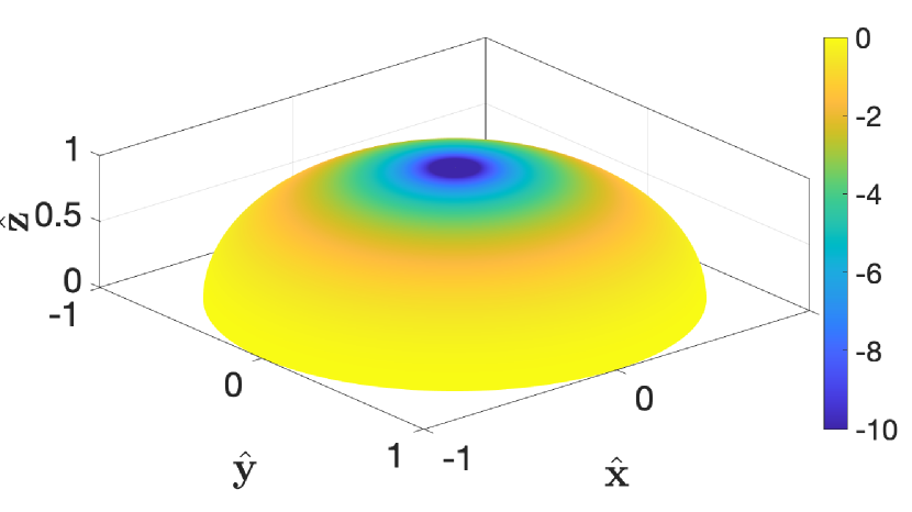
(a) Isotropic

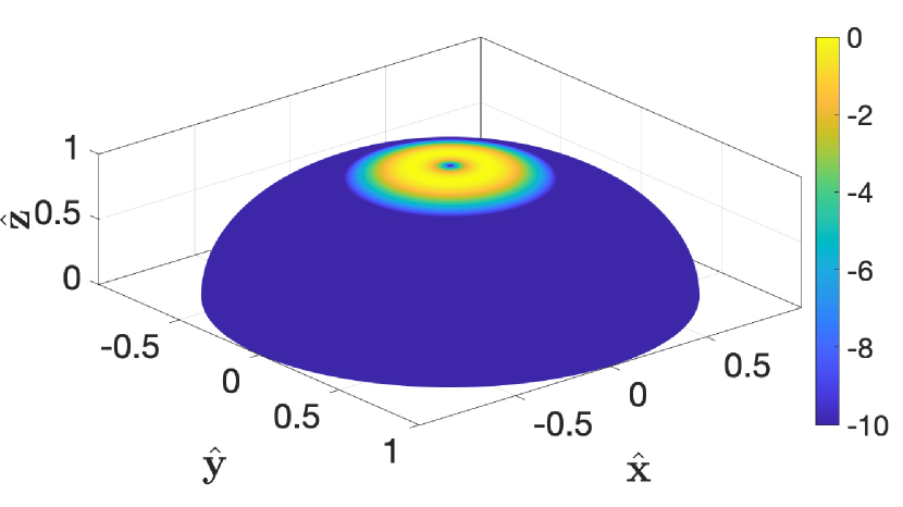
(b) Non-isotropic

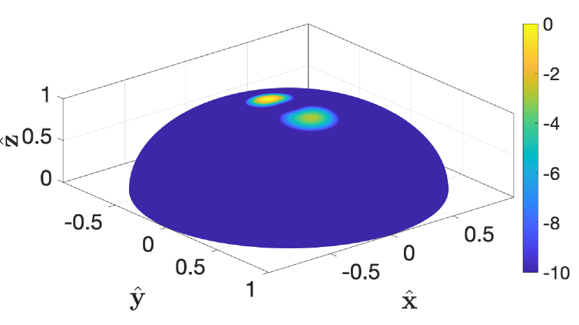
(c) Non-isotropic mixture

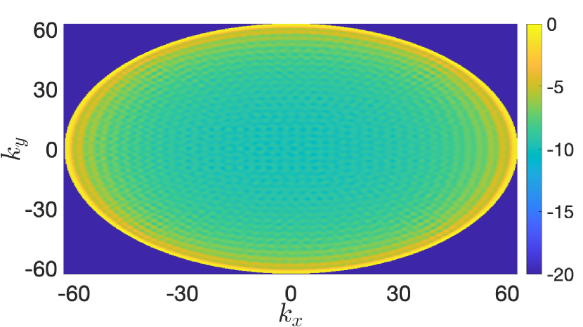
(d) Isotropic

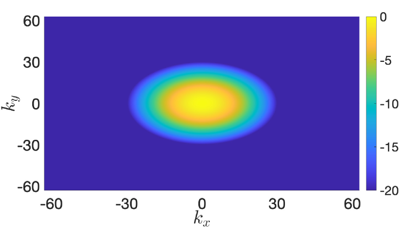
(e) Non-isotropic

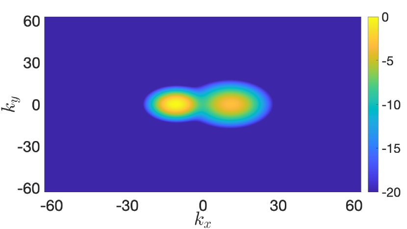
(f) Non-isotropic mixture

Figure 5: Scattering under isotropic and non-isotropic conditions. The first row shows the spectral factor $\sin(\theta)A(\theta,\phi)$ in (64) with $(\theta,\phi)\in[0,\pi/2]\times[0,2\pi)$. The second row shows the PSD $S(\mathbf{k})$ in (58).

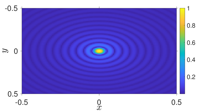
(a) Isotropic

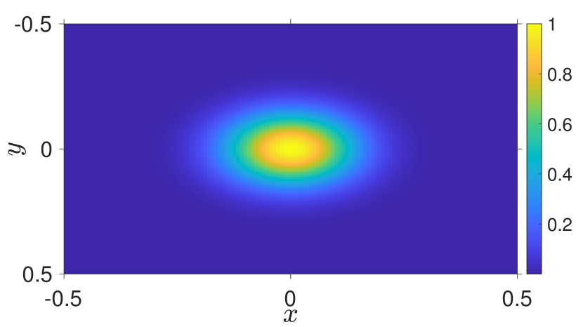
(b) Non-isotropic

(c) Non-isotropic mixture

Figure 6: ACF $c(\mathbf{r})$ in (62) under the scattering conditions of Fig. 5.

The autocorrelation function (ACF) $c(\mathbf{r})=\mathbb{E}\{e(\mathbf{r}^{\prime})e^{*}(\mathbf{r}^{\prime}+\mathbf{r})\}$ of $e(\mathbf{r})$ obeys the Helmholtz equation in (17) [22, Eq. (4)]:

$$\nabla^{2}c(\mathbf{r})+\kappa^{2}c(\mathbf{r})=0.$$ (56)

Here, the dependence on $z$ is removed as it is immaterial to the statistics of the field. An analogue procedure developed in Section III for a deterministic $e(\mathbf{r})$ yields [21, 22]:

$$c(\mathbf{r})=\frac{1}{(2\pi)^{2}}\int_{\mathbb{R}^{2}}S(\mathbf{k})e^{\mathsf{j}\mathbf{k}^{\mbox{\tiny$\mathrm{T}$}}\mathbf{r}}\,d\mathbf{k}$$ (57)

where the power spectral density (PSD) of $e(\mathbf{r})$ is defined as

$$S(\mathbf{k})=\frac{A^{2}(\mathbf{k})}{k_{z}(\mathbf{k})}\mathbbm{1}_{\mathcal{D}}(\mathbf{k})$$ (58)

with $A(\mathbf{k})$ being an arbitrary non-negative function, called spectral factor. Compared to (23), the integration region is restricted to $\mathbf{k}\in\mathcal{D}$ as $k_{z}(\mathbf{k})$ must be real-valued in order for $c(\mathbf{r})$ to satisfy the standard Hermitian-symmetry property.

The random field $e(\mathbf{r})$ is obtained by expanding a white-noise complex field $W(\mathbf{k})$ with unit variance over the same 2D Fourier basis in (57), which yields the Fourier spectral representation of $e(\mathbf{r})$ [21, Sec. III.C]:

$$e(\mathbf{r})=\frac{1}{2\pi}\int_{\mathbb{R}^{2}}{S^{1/2}(\mathbf{k})W(\mathbf{k})}e^{\mathsf{j}\mathbf{k}^{\mbox{\tiny$\mathrm{T}$}}\mathbf{r}}\,d\mathbf{k}$$ (59)

where equality must be understood in the MSE sense for any field with finite average energy [21]

$$\sigma^{2} =\int_{\mathbb{R}^{2}}\mathbb{E}\{|{e}(\mathbf{r})|^{2}\}\,d\mathbf{r}=\frac{1}{2\pi}\int_{\mathbb{R}^{2}}S(\mathbf{k})\,d\mathbf{k}.$$ (60)

We can interpret (59) as a 2D inverse Fourier transform of a wavenumber spectrum $E(\mathbf{k})={S^{1/2}(\mathbf{k})W(\mathbf{k})}$ consisting of a continuum of circularly symmetric complex Gaussian and statistically independent coefficients [21, 22].

VI-B DoF of Electromagnetic Random Fields

The computation of the DoF of a stationary random process requires to identify a basis set of functions that yields uncorrelated coefficients – also statistically independent for a jointly Gaussian process. This is at the basis of the Karhunen-Loeve series expansion [34, Sec. 3.3.2]. Finding this basis set is hard in practice, as an explicit solution is only available for a few cases. As an example, for a stationary random process $e(t)$ with a constant and bandlimited spectrum, it can be found by solving the Slepian’s concentration problem [32] [10, Sec. 2]. The same theory extends to a stationary random field $e(\mathbf{r})$ of constant and bandlimited spectrum [30],[10, Sec. 3].

A way to overcome the difficulty in finding a Karhunen-Loeve series expansion is to operate in the asymptotic regime. Particularly, as the observation interval $T$ of a stationary process $e(t)$ becomes large, for a given bandwidth $\Omega$, i.e., $\Omega T\gg 1$, the Karhunen-Loeve series expansion tends to a Fourier series expansion with statistically independent coefficients, whose variances are obtained by sampling the PSD of $e(t)$ [34, Sec. 3.4.6]. The translation of this result to the spatial domain is ensured by a time-frequency and space-wavenumber duality [20][21, Sec. V].

As the size $L$ of a squared observation region increases, for a given wavelength $\lambda$, i.e., $L/\lambda\gg 1$, a 2D Fourier series with fundamental frequency of $2\pi/L$ rad/m may be defined, which enjoys the same statistical independence properties [1]. As $L/\lambda\to\infty$, series are replaced by integrals like the one in (59) with continuous spectrum $E(\mathbf{k})$ replacing Fourier coefficients. The DoF are obtainable by counting the wavenumber lattice samples taken at $2\pi/L$ rad/m apart within the spectral support of $E(\mathbf{k})$. Under isotropic scattering, with spectral support given by the disk $\mathcal{D}$ of radius $\kappa=2\pi/\lambda$, this coincides to the Gauss circle problem [35].

VII Numerical Analysis

Numerical results are provided next to validate the above results on Nyquist sampling and field’s reconstruction. Simulations are carried out for a stationary electromagnetic random field under isotropic and non-isotropic scattering conditions, which are analytically modeled next.

VII-A Isotropic and Non-isotropic Scattering

In elevation and azimuth angles, (57) can be rewritten as

$$c(\mathbf{r}) \mathop{=}^{(a)}\int_{0}^{\frac{\pi}{2}}\!\!\!\int_{0}^{2\pi}\!\!\!A^{2}(\theta,\phi)e^{\mathsf{j}\mathbf{k}^{\mbox{\tiny$\mathrm{T}$}}(\theta,\phi)\mathbf{r}}\sin(\theta)d\theta d\phi$$ (61)

$$\mathop{=}^{(b)}\int_{0}^{\frac{\pi}{2}}\!\!\!\int_{0}^{2\pi}\!\!\!A^{2}(\theta,\phi)e^{\mathsf{j}\kappa\sin(\theta)(\cos(\phi)x+\sin(\phi)y)}\sin(\theta)d\theta d\phi$$ (62)

where $(a)$ is due to a change of variables with Jacobian $d\mathbf{k}/k_{z}(\mathbf{k})\propto\sin(\theta)d\theta d\phi$ and $(b)$ is obtained by substituting (28) [20]. Here, constant terms due to change of variables are embedded into $A^{2}(\theta,\phi)$.

An isotropic scattering scenario is modeled as $A(\theta,\phi)=1$ and plotted (inclusive of the Jacobian $\sin(\theta)$) in Fig. 5(a) on the upper hemisphere $(\theta,\phi)\in[0,\pi/2]\times[0,2\pi)$. In the wavenumber domain, we have that $A(\mathbf{k})=1$ so that the PSD in (58) is given by $S(\mathbf{k})=\mathbbm{1}_{\mathcal{D}}(\mathbf{k})/k_{z}(\mathbf{k})$, as we expected from the deterministic case in Fig. 3(a). This is plotted in Fig. 5(d). The isotropic ACF is shown in Fig. 6(a). This is computed from (62) by setting $x=\|\mathbf{r}\|$ and $y=0$ (due to polar symmetry),

$$c(\mathbf{r})=\mathrm{sinc}(2{\|\mathbf{r}\|}/{\lambda})$$ (63)

and coincides to the Clarke’s model [36, Sec. 2.4].

Non-isotropic scattering can be considered alike by specifying a non-uniform spectral factor $A(\theta,\phi)$. In this case, $A(\mathbf{k})$ (thus $S(\mathbf{k})$) will have arbitrary shape, as first assumed in the deterministic settings in Fig. 1. A clustered propagation environment is modeled as a mixture of spectral factors [20]

$$A^{2}(\theta,\phi)=\sum_{i=1}^{N_{\rm c}}w_{i}\,A^{2}_{i}(\theta,\phi)$$ (64)

weighted by $w_{i}\geq 0$ whose sums yields $1$. Here, $A^{2}_{i}(\theta,\phi)$ is representative of the $i$-th cluster. A simple way to model $A^{2}_{i}(\theta,\phi)$ is by using the 3D von Mises-Fisher distribution [20], parametrized by a modal direction

$$\hat{\boldsymbol{\xi}}_{i}=\begin{pmatrix}\sin({\theta_{r,i}})\cos({\phi_{r,i}})\\ \sin({\theta_{r,i}})\sin({\phi_{r,i}})\\ \cos({\theta_{r,i}})\end{pmatrix}$$ (65)

and an angular concentration ${\alpha_{i}\in[0,\infty)}$ describing the power spread around $\hat{\boldsymbol{\xi}}_{i}$. Clearly, isotropic scattering in Fig. 5(a) is obtained from (64) by setting ${N_{\rm c}=1}$ and ${\alpha=0}$. Non-isotropic scattering is considered in Fig. 5(b) and Fig. 5(c). In these cases, the support of $\mathcal{K}$ is measured by considering the bandwidth at $-20$ dB. We will see that this criterion provides an accurate measure of the field’s spectral support.

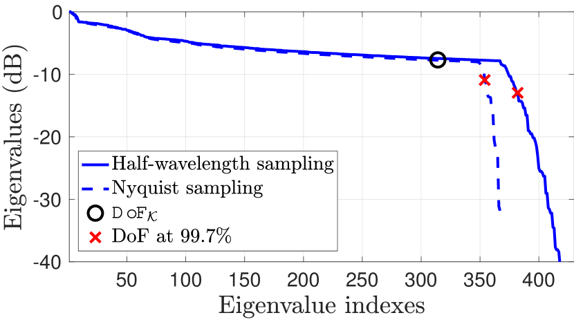
(a) Isotropic

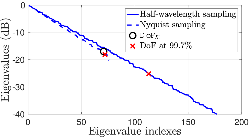
(b) Non-isotropic

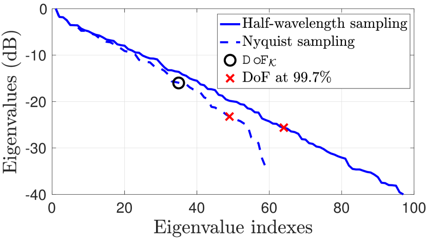
(c) Non-isotropic mixture

Figure 7: Eigenvalues of $\mathbf{C}$ (in dB) reported in a descending order under the scattering conditions depicted in Fig. 5. Nyquist samples of $e(\mathbf{r})$ are collected within a squared region $\mathcal{A}$ of side length $L=10\lambda$.

In Fig. 5(b), we have a single cluster with ${{\theta_{r}}={\phi_{r}}=0^{\circ}}$, and $\alpha=40$. The wavenumber domain is showed in Fig. 5(e) with circular support $\mathcal{K}$ of approximately $0.47\kappa$ radius, i.e., ${\sqrt{d_{1}}=\sqrt{d_{2}}=0.47}$, and $k_{\phi}=0$; see Fig. 1. The ACF is reported in Fig. 6(b) and shows a larger coherence area with respect to the isotropic case, due to a higher selectivity of the scattering.

In general, $\mathcal{K}$ has arbitrary shape – not necessarily circular – as first assumed in the deterministic settings in Fig. 1. This is shown in Fig. 5(c) and Fig. 5(f) in both representation domains for a two-clustered scenario with ${w_{1}=w_{2}=1/2}$, ${\theta_{r,1}=0^{\circ}}$, ${\theta_{r,2}=10^{\circ}}$, ${\phi_{r,1}=180^{\circ}}$, ${\phi_{r,2}=0^{\circ}}$, $\alpha_{1}=200$ and $\alpha_{2}=100$. We resort to an elliptical embedding with $\sqrt{d_{1}}=0.5$, $\sqrt{d_{2}}=0.35$, and $k_{\phi}=0$. The corresponding ACF is given in Fig. 6(c) and shows the impact of asymmetries in the PSD of $e(\mathbf{r})$.

VII-B Non-Asymptotic Regime

Electromagnetic fields are physically observable on a spatial region $\mathcal{A}\subset\mathbb{R}^{2}$ of finite size, from which only a finite number $N$ of samples is available for field’s reconstruction, and given by

$$N=\lceil\mathrm{dof}\rceil=m(\Lambda(\mathcal{A}))$$ (66)

where $\Lambda(\mathcal{A})\subseteq\mathbb{Z}^{2}$ denotes the truncated 2D lattice used for Nyquist sampling. The reconstruction formula obtained by truncating the 2D cardinal series expansion in (14) up to $N$ terms yields

$$\hat{e}(\mathbf{r})=\sum_{\mathbf{n}\in\Lambda(\mathcal{A})}e(\mathbf{Q}^{\star}\mathbf{n})f_{\mathcal{K}}(\mathbf{r}-\mathbf{Q}^{\star}\mathbf{n})$$ (67)

to which is associated a pointwise mean-squared error (MSE)

$$\sigma^{2}_{N}(\mathbf{r})=\mathbb{E}\{|{e}(\mathbf{r})-\hat{e}(\mathbf{r})|^{2}\}$$ (68)

where the expectation is taken with respect to all possible configurations of scatterers. The error magnitude is inevitably higher at the boundary region of $\mathcal{A}$, due to the truncation and non-orthogonality of the interpolating set of functions in (67) over $\mathbf{r}\in\mathcal{A}$. The accuracy of the reconstruction procedure in a non-asymptotic regime can be measured by the average energy of the error per unit of area [10]

$$\sigma^{2}_{N}=\frac{1}{m(\mathcal{A})}\int_{\mathcal{A}}\sigma^{2}_{N}(\mathbf{r})\,d\mathbf{r}$$ (69)

which tends to zero asymptotically as $N\to\infty$ (i.e., $\mathcal{A}=\mathbb{R}^{2}$), when (67) reduces to (14). Remarkably, under the Nyquist condition, the reconstruction formula (67) with the interpolating function (15) provides us with the best linear interpolator of $e(\mathbf{r})$ in the MSE sense [8, Sec. VI][9, Sec. III].

Also noteworthy is that the sampling operation of electromagnetic fields undergoes the same practical constraints imposed by hardware implementation issues (as for time-domain signals). For example, analog-to-digital converters can only provide a finite precision description of analog samples measured at every points, which inevitably introduces a quantization loss [12, Sec. 4.8]. Nevertheless, one way to compensate for these losses is to trade-off some efficiency by sampling above Nyquist density [37].

VII-C Sampling and Reconstruction in Non-Asymptotic Regime

\begin{overpic}[width=433.1833pt,tics=10]{Fig8a} \end{overpic}

(a) Isotropic scattering.

\begin{overpic}[width=433.1833pt,tics=10]{Fig8b} \end{overpic}

(b) Non-Isotropic scattering

Figure 8: Nyquist sampling plotted against the ACF $c(\mathbf{r})$.

To quantify the impact of Nyquist sampling and the number of DoF, we consider the eigenvalues of the spatial autocorrelation matrix ${\mathbf{C}\in\mathbb{C}^{N\times N}}$, obtained under the scattering conditions depicted in Fig. 5 and a squared region $\mathcal{A}$ of side length ${L=10\lambda}$. In the isotropic scenario, $\mathbf{C}$ is obtained by hexagonal sampling of (63) according to (34). For any non-isotropic scenario, we sample (62) by using the elongated hexagonal sampling in (42) with corresponding parameters. Comparisons are made with the (redundant) half-wavelength sampling in (30). The number of DoF is computed on the basis of the results in Section V and is numerically compared to the number of samples sufficient to capture $99.7\%$ of the total field’s power. This will be slightly higher because of the finite value of $L/\lambda$. As $L/\lambda$ increases, the eigenvalue curves assume a step-like function behavior with transition corresponding to the number of DoF approximately.

In Fig. 7(a), the isotropic case is studied. From (51), we obtain $\mathrm{dof}_{\mathcal{D}}=315$ while $354$ eigenvalues are obtained with the $99.7\%$ criterion. The number of DoF at $99.7\%$ with $\lambda/2$ sampling increases up to $382$. This is not due to oversampling but to the larger area covered with the rectangular sampling, compared to hexagonal sampling, since it is impossible to fit the hexagonal and rectangular grids within the same area. The non-isotropic cases are considered in Fig. 7(b) and Fig. 7(c). From (53), the number of DoF reduces to ${\mathrm{dof}_{\mathcal{K}}=71}$ and ${\mathrm{dof}_{\mathcal{K}}=35}$, which is due to the scattering selectivity that cuts off some of the resolvable propagation directions. Compared to Fig. 7(a), the eigenvalue curves decay rapidly due to the spatial correlation; see also Fig. 6. Differences between the two curves are again due to numerical comparison issues.

From Fig. 7(a), it follows that spatial correlation exists even under isotropic propagation (see also [33, Sec. IV]). This is because $c(\mathbf{r})$ is not sampled at its zeros, as illustrated in Fig. 8(a). The hexagonal sampling provides the best trade off between collecting uncorrelated samples and minimizing the search area. Hence, it is the one that exploits the available number of DoF per unit of area. The non-isotropic case is shown in Fig. 8(b) for completeness. As seen, to the higher correlation in Fig. 7(c), compared to the isotropic case, corresponds an increased difficulty in achieving the above trade off due to a larger coherence area of the ACF.

A numerical example is provided next to verify the reconstruction formula in (67) with interpolating function in (15), under the scattering conditions of Fig. 5(b) (Fig. 5(e)). Samples are obtained within a squared region $\mathcal{A}$ of finite size. In Fig. 9, we gather measurements from a square of dimension ${L/\lambda=40}$ to recover the real part of $e(\mathbf{r})$ within a segment of length $L/\lambda=6$ along the $x$-axis. Nyquist sampling (42) with ${\sqrt{d_{1}}=\sqrt{d_{2}}=0.47}$, and ${k_{\phi}=0}$ is compared to half-wavelength rectangular sampling. Sampling at Nyquist density achieves similar performance while saving $60\%$ of samples/m². Both have a non-zero error due to the finite number of samples exploited for reconstruction. Nevertheless, the error is small in both cases as only a tiny contribution to reconstruction is added by the tails of the interpolating functions.

The normalized MSE $\sigma^{2}_{N}/\sigma^{2}$, defined as the ratio between (68) and (60), is plotted in Fig. 10 (in dB) as a function of $L/\lambda\in[2,20]$. Nyquist sampling is compared to rectangular sampling with spacing $\sqrt{d_{1}}\lambda/2$; that corresponds to a minimal squared embedding of $\mathcal{K}$ in Fig. 5(e). Both are plotted against hexagonal and half-wavelength samplings. Oversampling provides a better reconstruction in the finite $L/\lambda$ regime. All curves monotonically decrease with $L/\lambda$, due to the larger dataset available, and merge at infinity where the MSE is zero.

\begin{overpic}[width=433.1833pt,tics=10]{Fig9} \end{overpic}

Figure 9: Reconstruction of the real part of $e(\mathbf{r})$ over a segment of length $L/\lambda=6$, under the scattering conditions of Fig. 5(b).

\begin{overpic}[width=433.1833pt,tics=10]{Fig10} \end{overpic}

Figure 10: Normalized MSE as a function of $L/\lambda\in[2,20]$.

VIII Conclusions

We applied signal processing tools such as the multidimensional sampling theorem and Fourier theory to study the Nyquist sampling and number of DoF of an electromagnetic field, under deterministic and stationary random scattering conditions. Starting from first principles of wave propagation theory, we showed that this is naturally modeled as a 2D bandlimited signal–without any prior low-pass filtering operation–whose bandwidth is determined by the richness of the underlying scattering mechanism. This is maximum under isotropic propagation, where the field is circularly bandlimited of radius inversely proportional to the wavelength. Hence, conventional signal processing techniques for bandlimited signals, e.g.,[12], can be applied to electromagnetic fields due to a fundamental space-time duality and linear system-theoretic interpretation of wave propagation.

For electrically large (i.e., relative to the wavelength) observation areas, the DoF per unit of area are the Nyquist samples per squared meters needed for reconstruction. With prior knowledge of the scattering conditions, we provided an efficient representation by solving an ellipse packing problem, which yields an elongated hexagonal sampling structure stretching inversely proportional to scattering selectivity. Under isotropic propagation, it leads to a $13\%$ less samples/m² compared to the classical half-wavelength sampling. This gap increases as the scattering becomes more selective angularly, thereby offering a substantial complexity reduction.

A possible extension of this paper is to consider nonuniform sampling [5]. In principle, this leads to another ellipse packing problem of equal sizes, but with arbitrary orientation and spacing, due to an irregular sampling structure.

Appendix A Proof of Lemma 1

From (15), for a wavenumber support $\mathcal{K}=\mathcal{D}$ we obtain

$$f_{\mathcal{D}}(\mathbf{r}) =\frac{|\det(\mathbf{Q}^{\star}_{\mathcal{D}})|}{(2\pi)^{2}}\int_{\mathcal{D}}e^{\mathsf{j}\mathbf{k}^{\mbox{\tiny$\mathrm{T}$}}\mathbf{r}}\,d\mathbf{k}$$ (70)

$$=\frac{1}{{2\sqrt{3}}}\int_{\|\mathbf{u}\|\leq 1}e^{\mathsf{j}\kappa\mathbf{u}^{\mbox{\tiny$\mathrm{T}$}}\mathbf{r}}\,d\mathbf{u}$$ (71)

where we applied a change of integration variables $\mathbf{u}=\kappa^{-1}\mathbf{I}_{2}\mathbf{k}=(u_{x},u_{y})$ and substituted $|\det(\mathbf{Q}^{\star}_{\mathcal{D}})|={\lambda^{2}}/({2\sqrt{3}})$ in (35) while using $\kappa=2\pi/\lambda$. Being (71) an inverse spatial Fourier transform of a rotationally symmetric spectrum, its result will be invariant under rotation, i.e., $f_{\mathcal{D}}(\mathbf{r})=f_{\mathcal{D}}(r)$ with $\|\mathbf{r}\|=r$. Hence, we evaluate (71) at the point $\mathbf{r}=(r,0)$:

$$f_{\mathcal{D}}(\mathbf{r}) =\frac{1}{\sqrt{3}}\int_{-1}^{1}e^{\mathsf{j}\kappa ru_{x}}\sqrt{1-u_{x}^{2}}\,du_{x}$$ (72)

$$\mathop{=}^{(a)}\frac{1}{\sqrt{3}}\int_{0}^{\pi}e^{\mathsf{j}\kappa r\cos(\theta)}\sin^{2}(\theta)\,d\theta$$ (73)

where in $(a)$ we applied a change of integration variables $u_{x}=\cos(\theta)$. By using the Euler’s formula and exploiting symmetry of the integrand we obtain

$$f_{\mathcal{D}}(\mathbf{r})=\frac{\pi}{\sqrt{3}}\frac{J_{1}(\kappa r)}{\kappa r}=\frac{\pi}{\sqrt{3}}\mathrm{jinc}(\kappa r)$$ (74)

where ${J_{1}(\alpha)\!=\!\frac{\alpha}{\pi}\!\!\int_{0}^{\pi}\!\!\cos(\alpha\cos(\theta))\sin^{2}(\theta)d\theta}$ [38, Eq. (9.1.20)].

Appendix B Proof of Lemma 3

From (15), for a wavenumber support $\mathcal{K}=\mathcal{E}$ we obtain

$$f_{\mathcal{E}}(\mathbf{r}) =\frac{|\det(\mathbf{Q}^{\star}_{\mathcal{E}})|}{(2\pi)^{2}}\int_{\mathcal{E}}e^{\mathsf{j}\mathbf{k}^{\mbox{\tiny$\mathrm{T}$}}\mathbf{r}}\,d\mathbf{k}$$ (75)

$$=|\det(\mathbf{G}^{1/2})|\frac{|\det(\mathbf{Q}^{\star}_{\mathcal{E}})|}{(2\pi)^{2}}\int_{\mathcal{D}}e^{\mathsf{j}(\mathbf{G}^{1/2}\mathbf{k}^{\prime})^{\mbox{\tiny$\mathrm{T}$}}\mathbf{r}}\,d\mathbf{k}^{\prime}$$ (76)

where we applied the change of integration variables ${\mathbf{k}^{\prime}=\varphi^{-1}(\mathbf{k})=\mathbf{G}^{-1/2}\mathbf{k}}$ with $\mathbf{k}^{\prime}\in\mathcal{D}$. Plugging (42),

$$f_{\mathcal{E}}(\mathbf{r}) =\frac{|\det(\mathbf{Q}^{\star}_{\mathcal{D}})|}{(2\pi)^{2}}\int_{\mathcal{D}}e^{\mathsf{j}(\mathbf{G}^{1/2}\mathbf{k}^{\prime})^{\mbox{\tiny$\mathrm{T}$}}\mathbf{r}}\,d\mathbf{k}^{\prime}.$$ (77)

Re-arranging the terms at the exponential of (77) to match (71) yields ${f_{\mathcal{E}}(\mathbf{r})=f_{\mathcal{D}}((\mathbf{G}^{1/2})^{\mbox{\tiny$\mathrm{T}$}}\mathbf{r})}$ Also, using (40) and exploiting the rotation invariance of $f_{\mathcal{D}}(\mathbf{r})$ yields $f_{\mathcal{E}}(\mathbf{r})=f_{\mathcal{D}}(\mathbf{D}^{1/2}\mathbf{r})$.

References

- [1] A. Pizzo, T. L. Marzetta, and L. Sanguinetti, “Degrees of freedom of Holographic MIMO channels,” in IEEE Int. Workshop Signal Process. Adv. Wireless Commun. (SPAWC), 2020, pp. 1–5.
- [2] C. Shannon, “Communication in the presence of noise,” Proc. IRE, vol. 37, no. 1, pp. 10–21, 1949.
- [3] J. M. Whittaker, “The “Fourier” theory of the cardinal function,” Proc. Edinburgh Math. Soc., vol. 1, no. 3, p. 169–176, 1928.
- [4] V. A. Kotel’nikov, On the Transmission Capacity of the “Ether” and Wire in Electrocommunications. Birkhäuser Boston, 2001.
- [5] M. Unser, “Sampling-50 years after shannon,” Proc. IEEE, vol. 88, no. 4, pp. 569–587, 2000.
- [6] R. Marks, Introduction to Shannon Sampling and Interpolation Theory. Springer-Verlag New York, 1991.
- [7] D. E. Dudgeon and R. M. Mersereau, Multidimensional Digital Signal Processing. Prentice Hall, 1990.
- [8] D. P. Petersen and D. Middleton, “Sampling and reconstruction of wave-number-limited functions in N-dimensional euclidean spaces,” Information and Control, vol. 5, no. 4, pp. 279–323, 1962.
- [9] H. Kunsch, E. Agrell, and F. Hamprecht, “Optimal lattices for sampling,” IEEE Trans. Inf. Theory, vol. 51, no. 2, pp. 634–647, 2005.
- [10] M. Franceschetti, Wave Theory of Information. Cambridge University Press, 2017.
- [11] M. D. Migliore, “Horse (electromagnetics) is more important than horseman (information) for wireless transmission,” IEEE Trans. Antennas Propag., vol. 67, no. 4, pp. 2046–2055, 2019.
- [12] A. V. Oppenheim and R. W. Schafer, Discrete-Time Signal Processing. Pearson, 2010.
- [13] T. S. Rappaport, Y. Xing, O. Kanhere, S. Ju, A. Madanayake, S. Mandal, A. Alkhateeb, and G. C. Trichopoulos, “Wireless communications and applications above 100 GHz: Opportunities and challenges for 6G and beyond,” IEEE Access, vol. 7, pp. 78 729–78 757, 2019.
- [14] O. Bucci and G. Franceschetti, “On the spatial bandwidth of scattered fields,” IEEE Trans. Antennas Propag., vol. 35, no. 12, pp. 1445–1455, 1987.
- [15] O. Bucci, C. Gennarelli, and C. Savarese, “Representation of electromagnetic fields over arbitrary surfaces by a finite and nonredundant number of samples,” IEEE Trans. Antennas Propag., vol. 46, no. 3, pp. 351–359, 1998.
- [16] A. S. Y. Poon, R. W. Brodersen, and D. N. C. Tse, “Degrees of freedom in multiple-antenna channels: a signal space approach,” IEEE Trans. Inf. Theory, vol. 51, no. 2, pp. 523–536, Feb 2005.
- [17] R. A. Kennedy, P. Sadeghi, T. D. Abhayapala, and H. M. Jones, “Intrinsic limits of dimensionality and richness in random multipath fields,” IEEE Trans. Signal Process., vol. 55, no. 6, pp. 2542–2556, 2007.
- [18] L. W. Hanlen and T. D. Abhayapala, “Space-time-frequency degrees of freedom: Fundamental limits for spatial information,” in IEEE Int. Symposium Inf. Theory (ISIT), 2007, pp. 701–705.
- [19] A. M. Sayeed, “Deconstructing multiantenna fading channels,” IEEE Trans. Signal Process., vol. 50, no. 10, 2002.
- [20] A. Pizzo, L. Sanguinetti, and T. L. Marzetta, “Spatial characterization of electromagnetic random channels,” IEEE Open J. Commun. Soc., vol. 3, pp. 847–866, 2022.
- [21] A. Pizzo, T. L. Marzetta, and L. Sanguinetti, “Spatially-stationary model for Holographic MIMO small-scale fading,” IEEE J. Sel. Areas Commun., vol. 38, no. 9, pp. 1964–1979, 2020.
- [22] T. L. Marzetta, “Spatially-stationary propagating random field model for Massive MIMO small-scale fading,” in IEEE Int. Symposium Inf. Theory (ISIT), June 2018, pp. 391–395.
- [23] T. L. Marzetta, “BLAST arrays of polarimetric antennas,” Nokia Proprietary, ITD-01-41984K, 2001.
- [24] S. Hu, F. Rusek, and O. Edfors, “Beyond massive mimo: The potential of data transmission with large intelligent surfaces,” IEEE Trans. Signal Process., vol. 66, no. 10, pp. 2746–2758, 2018.
- [25] E. Agrell and B. Csébfalvi, “Multidimensional sampling of isotropically bandlimited signals,” IEEE Signal Process. Lett., vol. 25, no. 3, pp. 383–387, 2018.
- [26] R. Kennedy and T. Abhayapala, “Source-field wave-field concentration and dimension: towards spatial information content,” in IEEE Int. Symposium Inf. Theory (ISIT), 2004, pp. 243–.
- [27] W. C. Chew, Waves and Fields in Inhomogenous Media. Wiley-IEEE Press, 1995.
- [28] J. Wang, “An examination of the theory and practices of planar near-field measurement,” IEEE Trans. Antennas Propag., vol. 36, no. 6, pp. 746–753, 1988.
- [29] D. A. B. Miller, “Communicating with waves between volumes: evaluating orthogonal spatial channels and limits on coupling strengths,” Appl. Opt., vol. 39, no. 11, pp. 1681–1699, Apr 2000.
- [30] M. Franceschetti, “On Landau’s eigenvalue theorem and information cut-sets,” IEEE Trans. Inf. Theory, vol. 61, no. 9, Sept 2015.
- [31] S. Boyd and L. Vandenberghe, Convex Optimization. USA: Cambridge University Press, 2004.
- [32] H. Landau and H. Widom, “Eigenvalue distribution of time and frequency limiting,” Journal of Mathematical Analysis and Applications, vol. 77, no. 2, pp. 469–481, 1980.
- [33] A. Pizzo, L. Sanguinetti, and T. L. Marzetta, “Fourier plane-wave series expansion for Holographic MIMO communications,” IEEE Trans. Wireless Commun., pp. 1–1, 2022.
- [34] H. L. Van Trees, Detection Estimation and Modulation Theory, Part I. Wiley, 1968.
- [35] E. W. Weisstein, “Gauss’s circle problem,” from MathWorld–A Wolfram Web Resource. [Online]. Available: https://mathworld.wolfram.com/GausssCircleProblem.html
- [36] A. Paulraj, R. Nabar, and D. Gore, Introduction to Space-Time Wireless Communications. Cambridge, UK: Cambridge University Press, 2003.
- [37] A. Kumar, P. Ishwar, and K. Ramchandran, “High-resolution distributed sampling of bandlimited fields with low-precision sensors,” IEEE Trans. Inf. Theory, vol. 57, no. 1, pp. 476–492, 2011.
- [38] M. Abramowitz and I. A. Stegun, Eds., Handbook of Mathematical Functions with Formulas, Graphs, and Mathematical Tables. U.S. Government Printing Office, 1972.