Influence of a spatial anisotropy on presence of the intermediate one-half magnetization plateau of a spin-1/2 Ising-Heisenberg branched chain

Abstract

A spin-1/2 Ising-Heisenberg branched chain constituted by regularly alternating Ising spins and Heisenberg dimers involving an additional side branching is exactly solved in a magnetic field by the transfer-matrix method. The spin-1/2 Ising-Heisenberg branched chain involves two different Ising and one Heisenberg coupling constants. The overall ground-state phase diagram is formed by three different ground states emergent depending on a mutual interplay between the magnetic field and three considered coupling constants: the modulated quantum antiferromagnetic phase, the quantum ferrimagnetic phase, and the classical ferromagnetic phase. It is shown that the interaction anisotropy connected to two different Ising coupling constants substantially influences a breakdown of the intermediate one-half magnetization plateau, which represents a macroscopic manifestation of the quantum ferrimagnetic phase.

1 Introduction

Quantum Heisenberg spin chains provide an intriguing platform for an investigation of quantum magnetism using fully rigorous calculation methods being completely free of any uncontrolled approximation [1]. A few exactly solved Ising-Heisenberg and Heisenberg branched spin chains have recently attracted considerable attention, because they may exhibit striking quantum critical points of Kosterlitz-Thouless and Gaussian type [2, 3, 4]. Moreover, the Ising-Heisenberg and Heisenberg branched spin chains are not only purely theoretical models, but they are closely related to a few real-world experimental realizations from the family of polymeric coordination compounds [5, 6]. In the present work we will investigate a spin-1/2 Ising-Heisenberg branched chain whose magnetic structure is inspired by the heterobimetallic coordination polymer [(Tp)₂Fe₂(CN)₆(OCH₃)(bap)Cu₂(CH₃OH)$\cdot$2CH₃OH] (Tp=tris(pyrazolyl)hydroborate, bapH = 1,3-bis(amino)-2-propanol) [6] to be further abbreviated as [Fe₂Cu₂]_∞.

2 Model and method

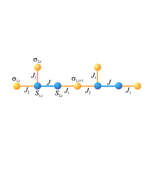
Figure 1: A schematic illustration of the spin-1/2 Ising-Heisenberg branched chain: orange (blue) circles denote lattice positions of the Ising (Heisenberg) spins.

The spin-1/2 Ising-Heisenberg branched chain, which is inspired by magnetic structure of the heterometallic coordination polymer [Fe₂Cu₂]_∞ originally reported in Ref. [6], can be defined through the Hamiltonian:

$$\hat{\cal{H}}\!\!\! = \!\!\!\displaystyle\sum_{i=1}^{N}\Bigl{\{}J\hat{\textbf{S}}_{1,i}\cdot\hat{\textbf{S}}_{2,i}+J_{1}\left(\hat{S}_{1,i}^{z}\hat{\sigma}_{2,i}^{z}+\hat{S}_{2,i}^{z}\hat{\sigma}_{1,i+1}^{z}\right)$$ (1)

$$+ \!\!\!J_{2}\hat{S}_{1,i}^{z}\hat{\sigma}_{1,i}^{z}-h\left(\hat{S}_{1,i}^{z}+\hat{S}_{2,i}^{z}+\hat{\sigma}_{1,i}^{z}+\hat{\sigma}_{2,i}^{z}\right)\Bigr{\}}.$$

Here, $\hat{\sigma}_{i}^{z}$ and $\hat{S}_{i}^{\alpha}$ ($\alpha=x,y,z$) are the spin-1/2 operators ascribed to the Ising and Heisenberg spins, which are schematically shown in Fig. 1 as orange and blue circles, respectively. This schematic illustration additionally involves also notation for three considered coupling constants: the coupling constant $J>0$ stands for the antiferromagnetic Heisenberg exchange interaction within the dimeric units from a backbone of the polymeric chain, while the coupling constants $J_{1}$ and $J_{2}$ correspond to two different Ising-type exchange interactions between the nearest-neighbor Ising and Heisenberg spins. Finally, the Zeeman’s term $h$ accounts for a magnetostatic energy of the Ising and Heisenberg spins in a magnetic field, $N$ is the total number of unit cells and the periodic boundary condition $\sigma_{1,N+1}\equiv\sigma_{1,1}$ is imposed for simplicity. For further convenience, the total Hamiltonian (1) can be rewritten as a sum of the cell Hamiltonians $\hat{\cal{H}}=\sum_{i=1}^{N}\hat{\cal{H}}_{i}$, where each cell Hamiltonian $\hat{\cal{H}}_{i}$ is defined by:

$$\hat{\cal{H}}_{i}\!\!\! = \!\!\!J\hat{\textbf{S}}_{1,i}\cdot\hat{\textbf{S}}_{2,i}+J_{1}\left(\hat{S}_{1,i}^{z}\hat{\sigma}_{2,i}^{z}+\hat{S}_{2,i}^{z}\hat{\sigma}_{1,i+1}^{z}\right)+J_{2}\hat{S}_{1,i}^{z}\hat{\sigma}_{1,i}^{z}$$ (2)

$$- \!\!\!h\left(\hat{S}_{1,i}^{z}+\hat{S}_{2,i}^{z}+\hat{\sigma}_{2,i}^{z}\right)-\frac{h}{2}(\hat{\sigma}_{1,i}^{z}+\hat{\sigma_{1,i+1}}).$$

The cell Hamiltonians $\hat{\cal{H}}_{i}$ obviously commute, i.e. $[\hat{\cal{H}}_{i},\hat{\cal{H}}_{j}]=0$, which means that the partition function of the spin-1/2 Ising-Heisenberg branched chain can be partially factorized into the following product:

$$\mathcal{Z}=\sum_{\{\sigma_{1,i}^{z}\}}\prod_{i=1}^{N}\sum_{\sigma_{2,i}^{z}}{\rm{Tr}}_{[S_{1,i},S_{2,i}]}{\rm{e}}^{-\beta\hat{\mathcal{H}}_{i}}=\sum_{\{\sigma_{1,i}^{z}\}}\prod_{i=1}^{N}{\rm{T}}(\sigma_{1,i}^{z},\sigma_{1,i+1}^{z}),$$

where $\beta=1/(k_{\rm{B}}T)$, $k_{\rm{B}}$ is the Boltzmann’s factor, $T$ is the absolute temperature, ${\rm{Tr}}_{[S_{1,i},S_{2,i}]}$ denotes a trace over degrees of freedom of the Heisenberg dimer from the $i$-th unit cell and $\sum_{\{\sigma_{1,i}^{z}\}}$ denotes a summation over all possible configurations of the Ising spins from a backbone of the branched chain. The expression ${\rm{T}}(\sigma_{1,i}^{z},\sigma_{1;i+1}^{z})={\rm{Tr}}_{[S_{1,i},S_{2,i}]}{\rm{e}}^{-\beta\hat{\mathcal{H}}_{i}}$ is the usual transfer matrix obtained after tracing out spin degrees of freedom of two Heisenberg spins and the Ising spin $\sigma_{2,i}$ from the $i$-th unit cell. To proceed further with the calculations, we have to calculate eigenvalues of the cell Hamiltonian (2) by performing a straightforward diagonalization in the local basis of the Heisenberg spins from the $i$-th unit cell:

$$\begin{split}E_{i1,i2}&=\frac{J}{4}\pm\frac{J_{1}}{2}\left(\sigma_{1,i}^{z}+\sigma_{1,i+1}^{z}\right)+\frac{J_{2}}{2}\sigma_{1,i}^{z}\mp h_{1},\\ E_{i3,i4}&=-\frac{J}{4}\pm\frac{1}{2}\sqrt{\left[\frac{J_{1}}{2}(\sigma_{2,i}^{z}+\sigma_{1,i+1}^{z})+\frac{J_{2}}{2}\sigma_{1,i}^{z}\right]^{2}+J^{2}},\end{split}$$

which should be shifted by the field term $-\frac{h}{2}\left(\sigma_{1,i}^{z}+\sigma_{1,i+1}^{z}\right)-h\sigma_{2,i}^{z}$ accounting for Zeeman’s energy of the Ising spins. The corresponding eigenvectors read

$$|\varphi_{i1}\rangle\!\!\! = \!\!\!|\!\uparrow\rangle_{1,i}|\!\uparrow\rangle_{2,i},\hskip 14.22636pt|\varphi_{i2}\rangle=|\!\downarrow\rangle_{1,i}|\!\downarrow\rangle_{2,i},$$

$$|\varphi_{i3}\rangle\!\!\! = \!\!\!c_{+}|\!\uparrow\rangle_{1,i}|\!\downarrow\rangle_{2,i}+c_{-}|\!\uparrow\rangle_{1,i}|\!\downarrow\rangle_{2,i},$$

$$|\varphi_{i4}\rangle\!\!\! = \!\!\!c_{+}|\!\uparrow\rangle_{1,i}|\!\downarrow\rangle_{2,i}-c_{-}|\!\uparrow\rangle_{1,i}|\!\downarrow\rangle_{2,i},$$ (3)

where

$$c_{\pm}=\frac{1}{\sqrt{2}}\sqrt{1\pm\frac{J_{1}\left(\sigma_{1,i+1}^{z}-\sigma_{2,i}^{z}\right)+J_{2}\sigma_{1,i}^{z}}{\sqrt{\left[J_{1}(\sigma_{1,i+1}^{z}-\sigma_{2,i}^{z})+J_{2}\sigma_{1,i}^{z}\right]^{2}+J^{2}}}}.$$ (4)

In this way one gets an explicit expression for the transfer matrix ${\rm{T}}(\sigma_{1,i}^{z},\sigma_{1;i+1}^{z})$:

$$\begin{split}{\rm{T}}(\sigma_{1,i}^{z}&,\sigma_{1;i+1}^{z})=\sum_{\sigma_{2,i}^{z}=\pm\frac{1}{2}}\sum_{j=1}^{4}{\rm{e}}^{-\beta E_{ji}}=2{\rm{e}}^{\frac{\beta h}{2}\left(\sigma_{1,i}^{z}+\sigma_{1,i+1}^{z}\right)-\frac{\beta J}{4}}\\ &\times\left\{{\rm{e}}^{\frac{\beta h}{2}}\cosh\left[\frac{\beta}{2}\left(J_{2}\sigma_{1,i}^{z}+J_{1}\sigma_{1,i+1}^{z}+\frac{J_{1}}{2}+2h_{1}\right)\right]\right.\\ &+{\rm{e}}^{-\frac{\beta h}{2}}\cosh\left[\frac{\beta}{2}\left(J_{2}\sigma_{1,i}^{z}+J_{1}\sigma_{1,i+1}^{z}-\frac{J_{1}}{2}+2h_{1}\right)\right]\\ &+{\rm{e}}^{\frac{\beta J}{2}+\frac{\beta h}{2}}\cosh\left[\frac{\beta}{2}\sqrt{\left(J_{2}\sigma_{1,i}^{z}\!-\!J_{1}\sigma_{1,i+1}^{z}+\frac{J_{1}}{2}\right)^{2}\!\!+J^{2}}\right]\\ &+\left.{\rm{e}}^{\frac{\beta J}{2}-\frac{\beta h}{2}}\cosh\left[\frac{\beta}{2}\sqrt{\left(J_{2}\sigma_{1,i}^{z}\!-\!J_{1}\sigma_{1,i+1}^{z}-\frac{J_{1}}{2}\right)^{2}\!\!+J^{2}}\right]\right\}.\end{split}$$ (5)

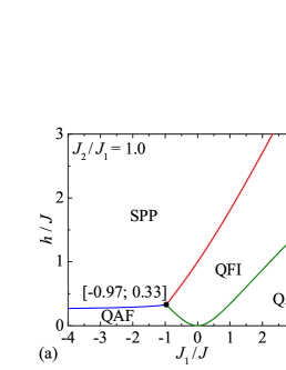
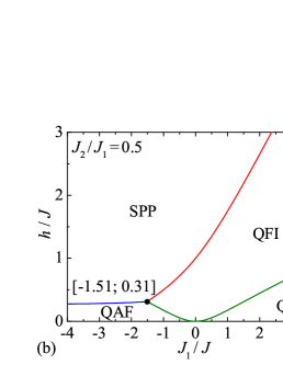
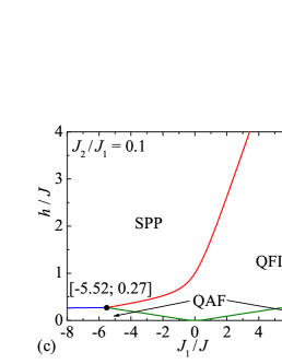
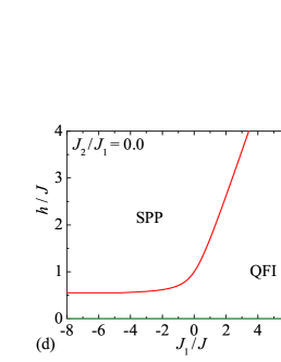
Figure 2: Ground-state phase diagrams of the spin-1/2 Ising-Heisenberg branched chain in the $J_{1}/J-h/J$ plane for four different values of the interaction ratio: (a) $J_{2}/J_{1}=1.0$; (b) $J_{2}/J_{1}=0.5$; (c) $J_{2}/J_{1}=0.1$; (d) $J_{2}/J_{1}=0.0$. The triple-point coordinates are given in square brackets.

The partition function of the spin-1/2 Ising-Heisenberg branched chain can be expressed in terms of two eigenvalues $\lambda_{+}$ and $\lambda_{-}$ of the transfer matrix (5):

$${\cal{Z}}=\sum_{\{\sigma_{1,i}\}}\prod_{i=1}^{N}{\rm{T}}\,(\sigma_{1,i}^{z},\sigma_{1;i+1}^{z})={\rm{Tr}}~{}{\rm{T}}^{N}=\lambda_{+}^{N}+\lambda_{-}^{N},$$ (6)

which can be written in this compact form:

$$\lambda_{\pm}=\frac{1}{2}\left[T_{1}+T_{2}\pm\sqrt{\left(T_{1}-T_{2}\right)^{2}+4T_{3}T_{4}}\right].$$ (7)

The parameters $T_{i}$ ($i=1-4$) mark four elements of two-by-two transfer matrix (5):

$$T_{1}={\rm{T}}(+,+),\,\,T_{2}={\rm{T}}(-,-),\,\,T_{3}={\rm{T}}(+,-),\,\,T_{4}={\rm{T}}(-,+),$$

which correspond to four possible states of the Ising spins $\sigma_{1,i}$ and $\sigma_{1,i+1}$ ($\pm$ applies for $\sigma=\pm 1/2$). In thermodynamic limit $N\rightarrow\infty$ the Gibbs free energy can be expressed through larger eigenvalue of the transfer matrix:

$$G=-k_{\rm{B}}T\lim_{N\rightarrow\infty}\frac{1}{N}\ln{\cal{Z}}=-k_{\rm{B}}T\ln\lambda_{+}.$$ (8)

Other quantities can be subsequently derived from the Gibbs free energy (8) using standard relations.

3 Results and discussion

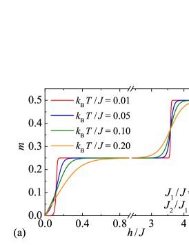
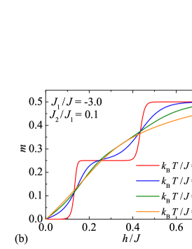
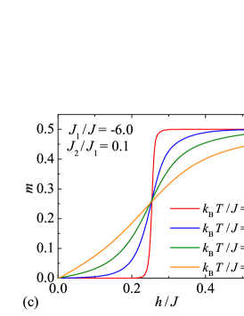
Figure 3: A few typical isothermal magnetization curves of the spin-1/2 Ising-Heisenberg branched chain for the fixed value of the interaction anisotropy $J_{2}/J_{1}=0.1$ and three different values of the interaction ratio: (a) $J_{1}/J=3.0$; (b) $J_{1}/J=-3.0$; (c) $J_{1}/J=-6.0$.

Let us begin discussion of the most interesting results by a comprehensive analysis of the ground state. It turns out that the spin-1/2 Ising-Heisenberg branched chain may exhibit just three different ground states referred to as the quantum antiferromagnetic phase (QAF):

$$|{\rm{QAF}}\rangle\!\!\!\! = \!\!\!\!\prod_{i=1}^{N/2}\!\left\{|\!\uparrow\rangle_{\sigma_{1,2i-1}}|\!\uparrow\rangle_{\sigma_{2,2i-1}}\!\left(a_{+}|\!\downarrow,\!\uparrow\rangle\!-\!a_{-}|\!\uparrow,\!\downarrow\rangle\right)_{S_{1,2i-1},S_{2,2i-1}}\right.$$

$$\otimes \!\!\!\!\left.\!|\!\downarrow\rangle_{\sigma_{1,2i}}|\!\downarrow\rangle_{\sigma_{2,2i}}\left(a_{-}|\!\downarrow,\!\uparrow\rangle\!-\!a_{+}|\!\uparrow,\!\downarrow\rangle\right)_{S_{1,2i},S_{2,2i}}\!\right\}\!,$$

the quantum ferrimagnetic phase (QFI):

$${|\rm{QFI}}\rangle=\prod_{i=1}^{N}|\!\uparrow\rangle_{\sigma_{1,i}}|\!\uparrow\rangle_{\sigma_{2,i}}\left(b_{+}|\!\downarrow,\!\uparrow\rangle\!-\!b_{-}|\!\uparrow,\!\downarrow\rangle\right)_{S_{1,i},S_{2,i}},$$

and the saturated paramagnetic phase (SPP):

$$|{\rm{SPP}}\rangle=\prod_{i=1}^{N}|\!\uparrow\rangle_{\sigma_{1,i}}|\!\uparrow\rangle_{\sigma_{2,i}}|\!\uparrow,\!\uparrow\rangle_{S_{1,i},S_{2,i}}.$$

For a shorthand notation the QAF and QFI ground states are defined through the probability amplitudes:

$$a_{\pm}=\frac{1}{\sqrt{2}}\sqrt{1\pm\frac{J_{1}+\frac{J_{2}}{2}}{\sqrt{\left(J_{1}+\frac{J_{2}}{2}\right)^{2}+J^{2}}}}$$ (9)

and

$$b_{\pm}=\frac{1}{\sqrt{2}}\sqrt{1\pm\frac{\frac{J_{2}}{2}}{\sqrt{\left(\frac{J_{2}}{2}\right)^{2}+J^{2}}}}.$$ (10)

It is worth mentioning that the QAF ground state with translationally broken symmetry is consistent with existence of zero magnetization plateau in a zero-temperature magnetization curve due to a null total magnetization, while the QFI ground state is responsible for presence of the intermediate one-half plateau if the total magnetization is scaled with respect to its saturation value.

The ground-state phase diagrams of the spin-1/2 Ising-Heisenberg branched chain are plotted in Fig. 2 in the $J_{1}/J-h/J$ plane for four selected values of the interaction anisotropy $J_{2}/J_{1}$. It can be concluded that the ground-state phase diagrams are formed regardless of the interaction anisotropy $J_{2}/J_{1}$ by the same three ground states QAF, QFI and SPP as previously reported in Ref. [4] for the isotropic case with $J_{2}/J_{1}=1$, see Fig. 2(a). The interaction anisotropy, i.e. the decline of the interaction ratio from the value $J_{2}/J_{1}=1$, merely causes an extension of the QFI ground state down to lower values of the interaction ratio $J_{1}/J$. On the other hand, the QAF ground state is gradually suppressed by the interaction anisotropy (i.e. when the interaction ratio $J_{2}/J_{1}$ decreases) until the QAF ground state completely disappears from the phase diagram in the limit $J_{2}/J_{1}\to 0$.

To verify the aforedescribed behavior, a few typical isothermal magnetization curves of the spin-1/2 Ising-Heisenberg branched chain are displayed in Fig. 3 for the fixed value of the interaction anisotropy $J_{2}/J_{1}=0.1$ and three selected values of the interaction ratio $J_{1}/J=3.0$, -3.0 and -6.0, respectively. It can be seen that a relatively wide one-half plateau and narrow zero plateau can be observed by considering the antiferromagnetic Ising coupling $J_{1}/J=3.0$ [see Fig. 3(a)], while the width of zero plateau extends and of one-half plateau shrinks by considering the ferromagnetic Ising coupling $J_{1}/J=-3.0$ [see Fig. 3(b)]. If the ferromagnetic Ising interaction is sufficiently strong one detects a mere existence of zero plateau and a full breakdown of the one-half plateau (see Fig. 3(c) for $J_{1}/J=-6.0$). It is noteworthy that the depicted magnetization curves are in a perfect accordance with the established ground-state phase diagrams (c.f. Figs. 2 and 3), whereby the intermediate one-half plateau is absent if a relative strength of the ferromagnetic Ising coupling constant exceeds the particular value ascribed to a triple coexistence point of the QAF, QFI and SPP ground states.

4 Conclusion

In the present paper we have exactly solved using the transfer-matrix method the spin-1/2 Ising-Heisenberg branched chain with two different Ising and one Heisenberg coupling constants in a magnetic field. It has been verified that the investigated quantum spin chain may exhibit just three different ground states QAF, QFI and SPP depending on a mutual interplay between the magnetic field and three considered coupling constants. The QAF and QFI ground states with a quantum entanglement between the Heisenberg dimers are responsible for presence of intermediate zero and one-half plateaus in zero- and low-temperature magnetization curves, whereby a relative size of the intermediate magnetization plateaus depends basically on the interaction anisotropy. A full breakdown of the intermediate one-half magnetization plateau has been additionally detected for the particular case with sufficiently strong ferromagnetic Ising coupling constants.

References

- [1] D.C. Mattis, The Many-Body Problem, World Scientific, Singapore, 1993.
- [2] L.M. Veríssimo, M.S.S. Pereira, J. Strečka, M.L. Lyra, Phys. Rev. B 99 (2019) 134408
- [3] F. Souza, L.M. Veríssimo, J. Strečka, M.L. Lyra, M.S.S. Pereira, Phys. Rev. B 102 (2020) 064414
- [4] K. Karl’ová, J. Strečka, M.L. Lyra, Phys. Rev. E 100 (2019) 042127.
- [5] H. Wang, L.-F. Zhang, Z.-H. Ni, W.-F. Zhong, L.-J. Tian, J. Jiang, Cryst. Growth Des. 10 (2010) 4231.
- [6] L.-C. Kang, X. Chen, H.-S. Wang, Y.-Z. Li, Y. Song, J.-L. Zuo, X.-Z. You, Inorg. Chem. 49 (2010) 9275.