The reverse flow and amplification of heat in a quantum-dot system

Abstract

We demonstrate that when a quantum dot is embedded between the two reservoirs described by different statistical distribution functions, the reverse flow and amplification of heat can be realized by regulating the energy levels of the quantum dot and the chemical potentials of two reservoirs. The reverse heat flow and amplification coefficient of the quantum device are calculated. The novelty of this device is that the reverse flow of heat does not need externally driving force and this seemingly paradoxical phenomenon does not violate the laws of thermodynamics. It is further expounded that the quantum device has some practical applications. For example, the device can work as a micro/nano cooler. Moreover, the performance characteristics of the cooler are revealed for different distribution functions. The coefficients of performance of the cooler operated at different conditions are calculated and the optimum selection criteria of key parameters are supplied.

PACS numbers

05.90. +m, 05.70. –a, 03.65.–w, 51.30. +i

I introduction

Thermal management devices aim to flexibly regulate the heat flow in a way similar to electronic devices controlling electrical current (key-1, 1, 2, , ). The fundamental modes of heat flow controls include thermal diodes (key-5, ; key-6, ; key-7, ), regulators (key-8, ; key-9, ; key-10, ), and switches (key-11, ; key-12, ; key-13, ), which have important applications in heating, cooling, and energy conversion. Quantum dots (QDs) as perfect energy filters due to their discrete electronic states are of significant interest for designing thermal management devices (key-14, ; key-15, ; key-16, ; key-17, ).

Inserting a QD into a semiconductor nanowire, Josefsson et al. demonstrated a quantum heat engine operating close to the thermodynamic efficiency limit (key-18, ; key-19, ). Dutta et al. made a tunable heat valve gate by controlling the heat flow in a Kondo-correlated single-quantum-dot transistor (key-20, ; key-21, ). Zhang et al. proposed a quantum thermal transistor based on three Coulomb-coupled quantum dots (key-22, ; key-23, ). Jaliel et al. experimentally realized a resonant tunneling energy harvester by connecting two quantum dots in series with a hot cavity (key-24, ). Considering a serial double quantum dot coupled to two electron reservoirs, Dorsch et al. showed that phonon-assisted transports enable the conversion of heat into electrical power in an energy harvester (key-25, ). These existing researches have laid the foundation for the concept design and experimental development of new quantum devices. Now, we consider one simple novel quantum device, where a QD with a single transition energy is embedded in the middle of two reservoirs described by different statistical distribution functions. It will be proved that such a device can transfer heat from a low temperature reservoir to a high temperature reservoir without external driving force and the amplification of heat flow can be realized in the transfer process.

The concrete contents of the paper are organized as follows: In Sec. II, we establish the model of a quantum-dot device, which may realize the reverse flow of heat. By applying the master equation approach, the thermodynamic characteristics of the quantum device operating between two Fermi or two Bose reservoirs are revealed. In Sec. III, the reverse flow and amplification of heat are realized by reasonably adjusting the energy levels of the quantum dot and the chemical potentials of two reservoirs. In Sec. IV, it is expounded that the quantum device can work as a micro/nano cooler. The coefficients of performance of the cooler operated at different conditions are calculated and the optimum operation regions of the cooler are determined. Finally, some meaningful conclusions are drawn.

II The model description of a single quantum-dot device

Figure 1 shows the model of a single quantum-dot system. It is made up of a QD with two energy levels and two reservoirs described by the distribution function

$$n_{\alpha}(E)=\frac{1}{\exp\left(\frac{E-\mu_{\alpha}}{k_{B}T_{\alpha}}\right)+\xi},$$ (1)

where $T_{\alpha}(T_{h}>T_{c})$ and $\mu_{\alpha}$ are, respectively, the temperature and chemical potential of reservoir $\alpha(=h,c)$, $k_{B}$ is Boltzmann’s constant, and $E$ is the transition energy corresponding the energy difference of the empty and filled states of the QD. For fermions, classical particles, and bosons, $\xi=1$, $0$, and $-1$, respectively. $q_{c}$ is the heat flow flowing from reservoir $c$ to the QD. $q_{h}$ is the heat flow flowing into reservoir $h$ through the QD. $\Gamma_{a}$ is the coupling strength between the QD and reservoir $\alpha$, which is a constant under the wideband approximation (key-26, ).

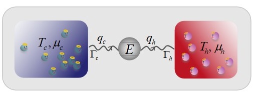
Figure 1: The schematic diagram of a two-level QD embedded between the hot reservoir $h$ and the cold reservoir $c$.

The free Hamiltonian of the QD in Fig.1 is given by

$$H=\frac{E}{2}\sigma^{z},$$ (2)

where $\sigma^{z}$ denotes the component of the Pauli operator in the z direction. The QD exchanges electrons with the nearby reservoirs at energy level $E$. Let $\rho_{0}(\rho_{1})$ denote the probability of finding the QD to be in empty (filled) state. Based on the Pauli master equation (key-26, ), the dynamics equation governing the evolution of the QD is given by

$$\frac{d}{dt}\left(\begin{array}[]{c}\rho_{0}\\ \rho_{1}\end{array}\right)=\left(\begin{array}[]{cc}-P_{10}(E)&P_{01}(E)\\ P_{10}(E)&-P_{01}(E)\end{array}\right)\left(\begin{array}[]{c}\rho_{0}\\ \rho_{1}\end{array}\right),$$ (3)

where the effective transmission rates $P_{10}(E)=\sum_{\alpha=h,c}\Gamma_{a}n_{a}(E)$ and $P_{01}(E)=\sum_{\alpha=h,c}\Gamma_{a}\bar{n}_{\alpha}(E)$. For a Fermi reservoir, $\bar{n}_{\alpha}(E)=1-n_{\alpha}(E)$. For a Bose reservoir, $\bar{n}_{\alpha}(E)=1+n_{\alpha}(E)$. Note that $E$ is required to be larger than zero, because quantum coherence caused by $E=0$ may influence the steady probability distribution so that Eq. (3) loses its efficacy (key-27, ). Equation (3) has a very simple interpretation: the rate of a particle tunneling into the QD from reservoir $\alpha$ is given by the bare tunneling rate $\Gamma_{\alpha}$ multiplied by the distribution function $n_{\alpha}(E)$. The rate of the inverse process, i.e., the tunneling of a particle from the QD into reservoir $\alpha$, is given by the product of $\Gamma_{\alpha}$ and $\bar{n}_{\alpha}(E)$.

By using Eq. (3) and the relation $\rho_{0}+\rho_{1}=1$, the particle current flowing from reservoir $c$ through the QD to reservoir $h$ is (key-17, ; key-28, )

$$I_{M}^{c}=a_{0}\left[n_{c}(E)-n_{h}(E)\right],$$ (4)

where $a_{0}=\Gamma_{h}\Gamma_{c}/\left(\Gamma_{h}+\Gamma_{c}\right)$ for fermions and $a_{0}=\Gamma_{h}\Gamma_{c}/\left(\Gamma_{h}S_{h}+\Gamma_{c}S_{c}\right)$ with $S_{\alpha}=1+2n_{\alpha}(E)$ for bosons. Eq. (4) satisfies the relation $I_{M}^{c}=-I_{M}^{h}$, where $I_{M}^{h}$ is the particle current removing from reservoir $h$ through the QD to reservoir $c$.

Each particle carries away an energy $E-\mu_{\alpha}$, when leaving reservoir $\alpha$ through the QD (key-29, ). Thus, the heat flows $q_{c}$ and $q_{h}$ are given by

$$q_{c}=\left(E-\mu_{c}\right)I_{M}^{c}$$ (5a)

and

$$q_{h}=\left(\mu_{h}-E\right)I_{M}^{h},$$ (5b)

respectively. Equation (5) shows that the particle and heat flows are proportional to each other. According to Eqs. (4) and (5), $n_{c}(E)-n_{h}(E)$, which is the difference between the distribution functions of reservoirs $c$ and $h$ at energy $E$, is one of the main factors in determining the directions of the particle and heat flows. At steady state, we are interested to reveal the mechanism of the reverse heat flow of the device, which requires the heat flowing out of the cold reservoir to be positive, i.e., $q_{c}>0$.

The rate of entropy production $\dot{S}$ of the device can be obtained by

$$\dot{S}=\frac{q_{h}}{T_{h}}-\frac{q_{c}}{T_{c}}=a_{0}\left(x_{c}-x_{h}\right)\left[n_{h}(E)-n_{c}(E)\right],$$ (6)

where $x_{\alpha}=\left(E-\mu_{\alpha}\right)/T_{a}$. According the second law of thermodynamics, $\dot{S}$ has to be not less than zero, i.e., $\dot{S}>0$.

Using Eq. (1), one can plot the curves of the distribution functions of the two reservoirs consisting of fermions, classical particles, and bosons varying with the transport mode $E$, as shown in Fig. 2. For any given type of particles, the curves of the distribution functions of reservoirs $c$ and $h$ intersect at energy $E_{0}=\left(T_{h}\mu_{c}-\mu_{h}T_{c}\right)/\left(T_{h}-T_{c}\right)$ (key-30, ; key-31, ). Figures 2$(a)$ and $(b)$ indicate, respectively, the cases of $\mu_{h}<\mu_{c}$ and $\mu_{h}>\mu_{c}$. For the case of $\mu_{h}>\mu_{c}$, $E_{0}<E<\mu_{c}$ and the distribution functions of two Bose reservoirs are negative, which are not plotted in Fig. 2$(b)$. Therefore, the system consisting of a single QD and two Bose reservoirs cannot realize the reverse flow of heat for $\mu_{h}>\mu_{c}$. Such a case will not be discussed below. Figure 2 shows that for different distribution functions, $E_{0}/\mu_{c}$ has a same value, which depends directly on the temperatures and chemical potentials. For example, for the parameter values given in Fig. 2, $E_{0}/\mu_{c}=1.15$ for the case of $\mu_{h}<\mu_{c}$ and $E_{0}/\mu_{c}=0.89$ for the case of $\mu_{h}>\mu_{c}$. Because the Maxwell–Boltzmann distribution function is a limit case of the Fermi-Dirac distribution function, the results related to the Maxwell–Boltzmann distribution function may be directly derived from those related to the Fermi-Dirac distribution function. Thus, the case of the Maxwell–Boltzmann distribution function will be not discussed below.

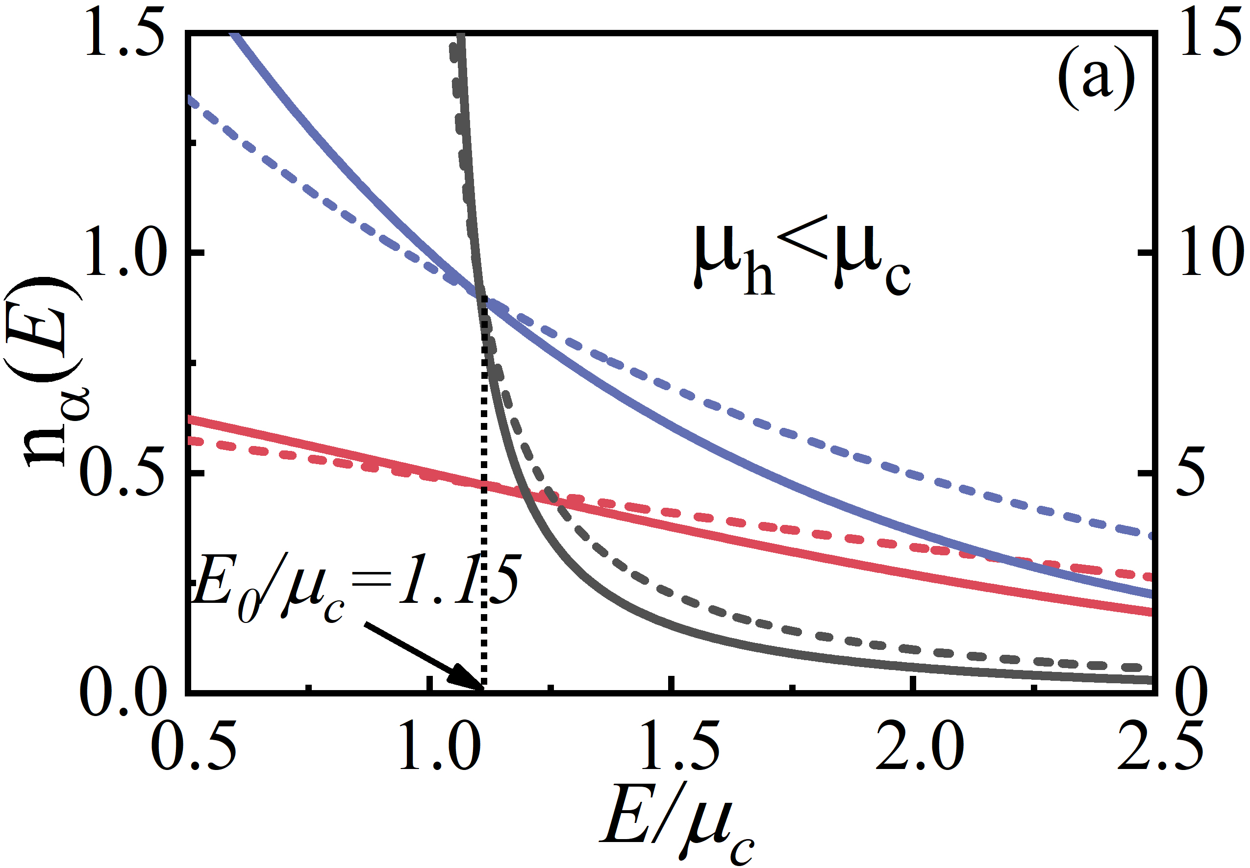
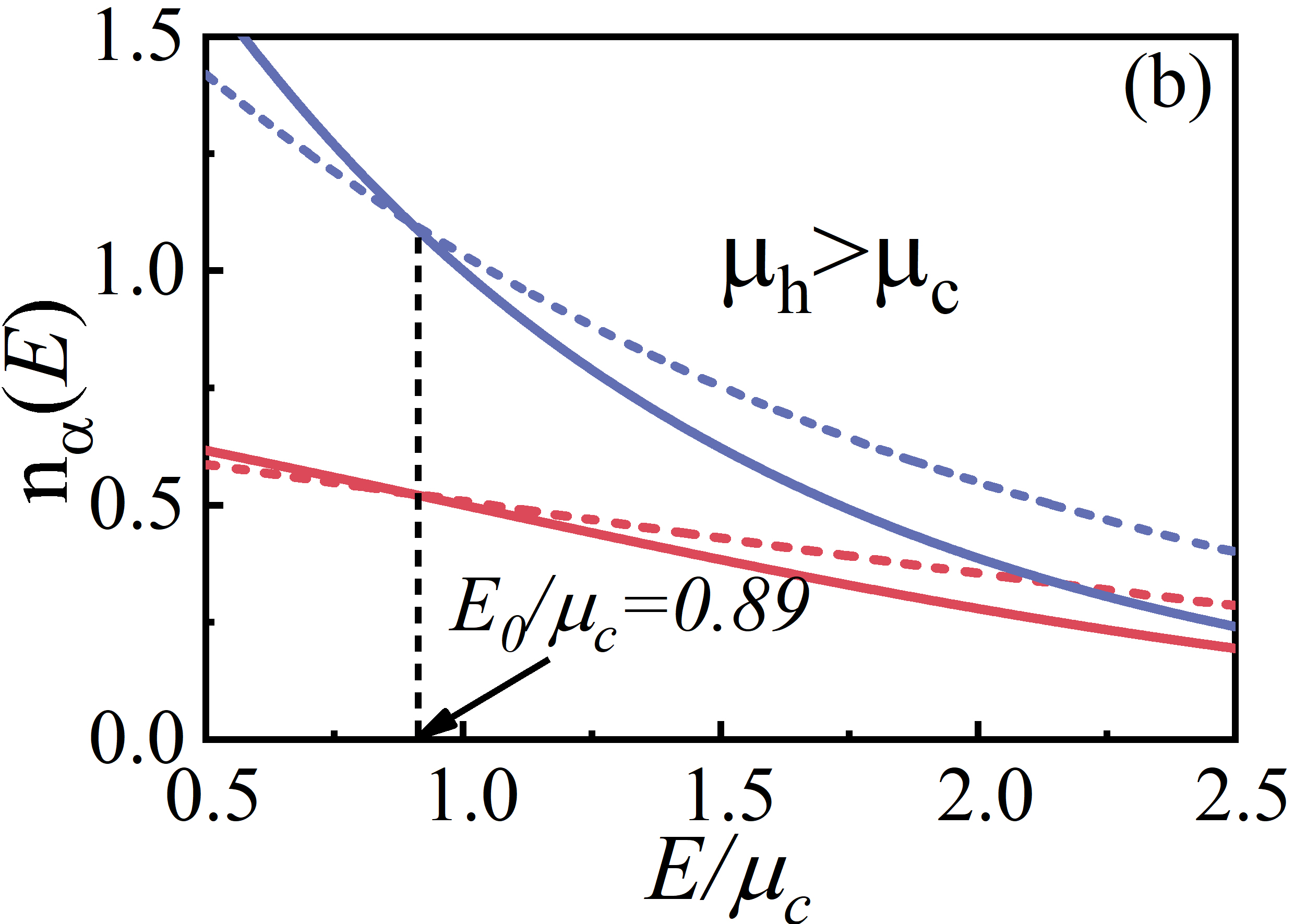
Figure 2: The curves of different distribution functions varying with $E/\mu_{c}$. The solid lines represent the mean occupation number $n_{c}(E)$ for reservoir $c$ at low temperature, while the dashed lines are the counterpart $n_{h}(E)$ for reservoir $h$ at high temperature. The black, red, and blue lines indicate the Bose-Einstein, Fermi-Dirac, and Maxwell–Boltzmann functions, respectively. The left vertical axis shows values for Fermi-Dirac and Maxwell–Boltzmann functions, while the corresponding scales of Bose-Einstein function are on the right vertical axis. The mean occupation numbers of reservoirs $h$ and $c$ at $E_{0}$ are equal, i.e., $n_{h}\left(E_{0}\right)=n_{c}\left(E_{0}\right)$. The parameters $T_{h}=3$ and $T_{c}=2$, (a) $\mu_{h}=1.9$ and $\mu_{c}=2$, and (b) $\mu_{h}=2$ and $\mu_{c}=1.9$ are chosen. In addition, Planck’s units are used by setting $\hbar=1$ and $k_{B}=1$ (key-32, ; key-33, ).

It is seen from Eqs. (4) and (5) that when particles are only transported at energy $E_{0}$, both the particle and heat flows vanish, the rate of entropy production $\dot{S}=0$, and the device can be operated reversibly. Note that $E=E_{0}$ is equivalent to $x_{h}=x_{c}$. This shows that the condition of $E=E_{0}$ does not require the temperatures and chemical potentials of two reservoirs to be identical.

According to the above analyses, we can further plot Fig. 3, which determines the operative regions of the single QD with the reverse flow of heat. In Fig. 3, the vertical, horizontal, and slash dashed lines represent the lines of $\mu_{h}/\mu_{c}=1$, $E_{0}/\mu_{c}=1$, and $E_{0}/\mu_{c}$ within $\left[0,T_{h}/\left(T_{h}-T_{c}\right)\right]$, respectively. Region I is bounded by the ordinate, the horizontal, and slash dashed lines. In region I, $\mu_{h}<\mu_{c}$ , $\mu_{c}<E<E_{0}$, and $n_{h}(E)<n_{c}(E)$, such that a positive particle current $I_{M}^{c}>0$ leaves the cold reservoir and there is a reverse flow of heat with $q_{c}>0$. It shows that the single QD operates between two Fermi (Bose) reservoirs with $\mu_{h}<\mu_{c}$, heat can be extracted from the low-temperature reservoir. Region II is bounded by the three lines of $E_{0}/\mu_{c}=1$, slash dashed line, and abscissa, while the right margin of Region II will be determined below. In region II, $\mu_{h}>\mu_{c}$ , $\mu_{c}>E>E_{0}$, and $n_{h}(E)>n_{c}(E)$, such that a negative particle current $I_{M}^{c}<0$ leaves the low-temperature reservoir and there is a reverse flow of heat $q_{c}>0$. It shows that when the single QD operates between two Fermi reservoirs with $\mu_{h}>\mu_{c}$, the heat of the low-temperature reservoir can be also extracted.

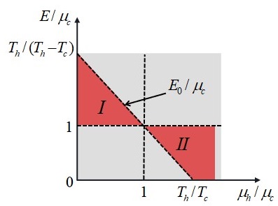
Figure 3: The operative regions of the single QD device with a non-zero reverse flow of heat. Region I is suitable for Fermi and Bose reservoirs. Region II is only suitable for Fermi reservoirs.

Figure 3 implies the fact that when the parameters of the QD and reservoirs satisfy the following relation

$$\mu_{h}/\mu_{c}<1<E/\mu_{c}<E_{0}/\mu_{c}$$

or

$$E_{0}/\mu_{c}<E/\mu_{c}<1<\mu_{h}/\mu_{c},$$

the device in Fig. 1 can have a non-zero reverse flow of heat.

III The reverse flow and amplification of heat

In the previous section, the necessary conditions for the reverse flow of heat have been illustrated. It’s important to choose the appropriate transition energy of the QD and the temperatures and chemical potentials of reservoirs. By using Eqs. (4)-(6), the three-dimension graphs of heat flow $q_{c}$, particle current $I_{M}^{c}$, and rate of entropy production $\dot{S}$ of the single QD system operating between two Fermi reservoirs varying with $E/\mu_{c}$ and $\mu_{h}/\mu_{c}$ are shown in Figs. 4(a)-(c), respectively. It is seen from Figs. 4(a)-(c) that when $\mu_{h}/\mu_{c}<1<E/\mu_{c}<E_{0}/\mu_{c}$, $q_{c}>0$, $I_{M}^{c}>0$, $\dot{S}>0$, and the device operates in region I in Fig. 3. This reveals the fact that an amount of heat is released from the low temperature reservoir, accompanied by the release of the particle current from the low temperature bath due to the chemical potential difference.

Similarly, when $E_{0}/\mu_{c}<E/\mu_{c}<1<\mu_{h}/\mu_{c}$, $q_{c}>0$, $I_{M}^{c}<0$, $\dot{S}>0$, and the device operates in region II in Fig. 3. The releasing of heat from the cold reservoir is accompanied by the particle current flowing into the cold reservoir. It shows that the device operating in regions I and II in Fig. 3 have a non-zero reverse flow of heat. It is found that $q_{c}$ is not a monotonic function of $E/\mu_{c}$ in regions I and II. When $E=E_{0}$, $q_{c}=0$ and $\dot{S}=0$, because the mean occupation numbers $n_{h}\left(E_{0}\right)=n_{c}\left(E_{0}\right)$ and the equal particles are transported reversibly between two reservoirs $h$ and $c$. When $E=\mu_{c}\neq\mu_{h}$, $\quad Q_{c}=0$, but $I_{M}^{c}\neq 0$ and $\dot{S}>0$. Fig. 4(a) shows that there exists a local maximum of $q_{c}$ in regions I. However, in region II, the maximum of $q_{c}$ increases with the increase of $\mu_{h}/\mu_{c}$, but it also has an upper bound. This problem will be discussed below.

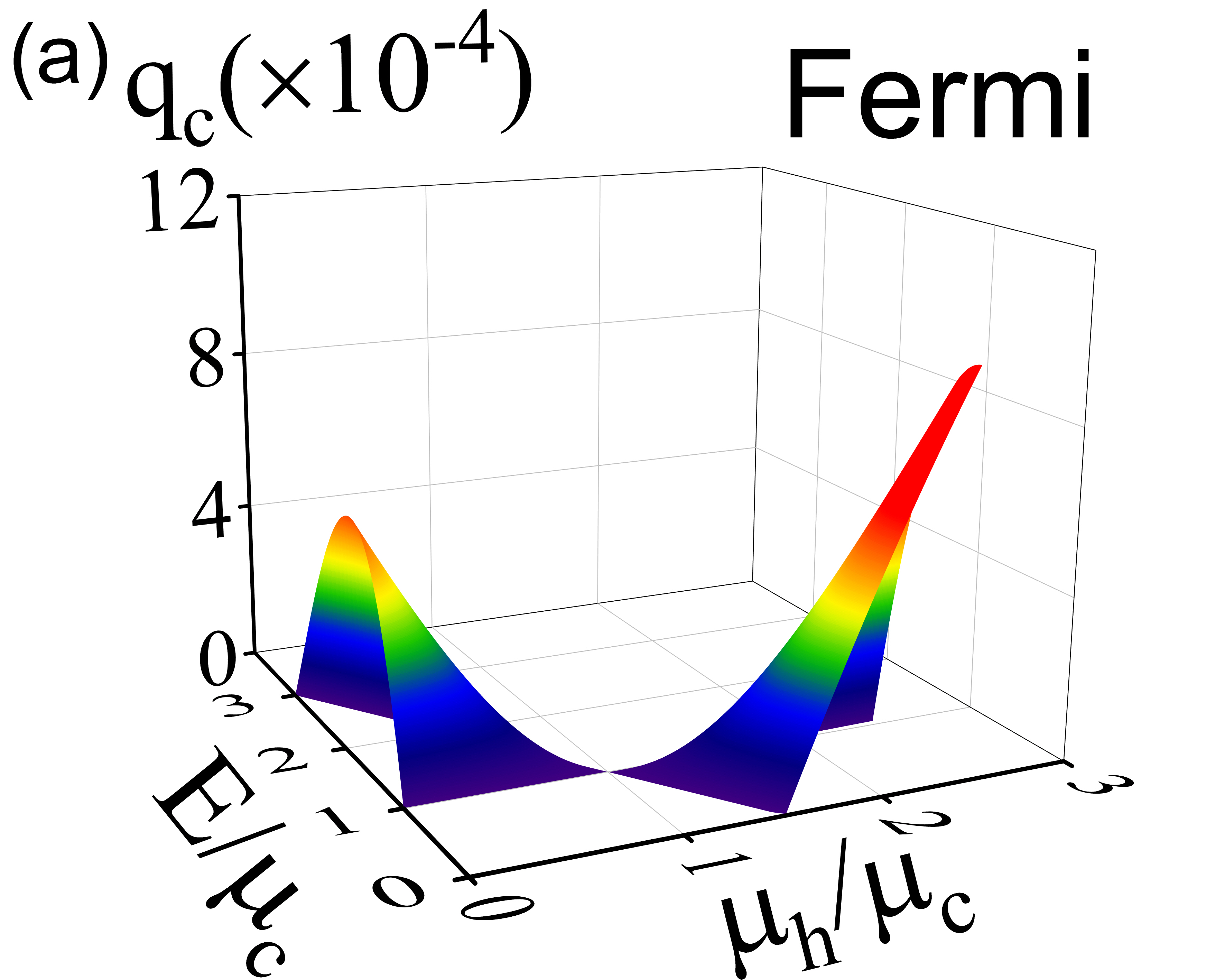
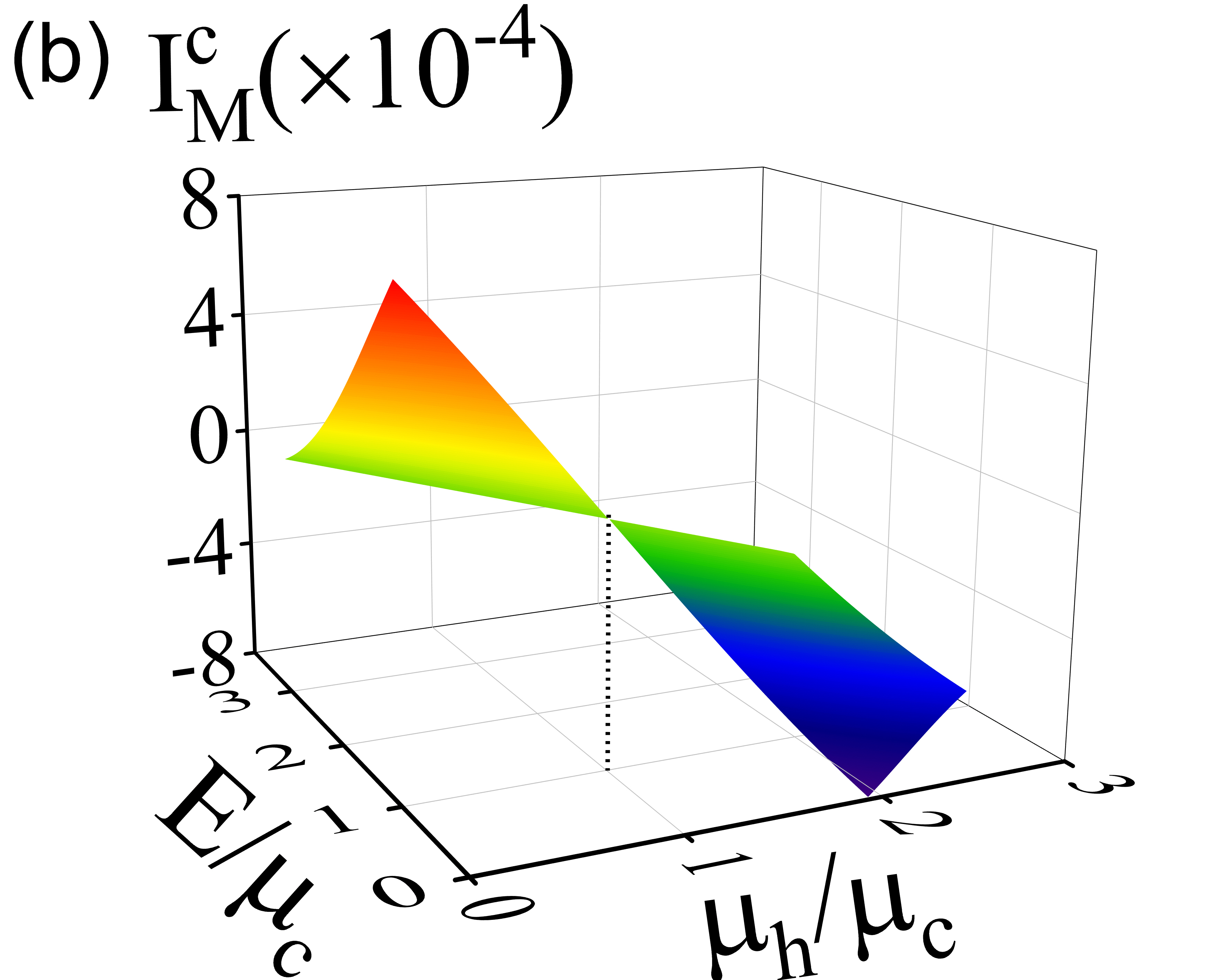
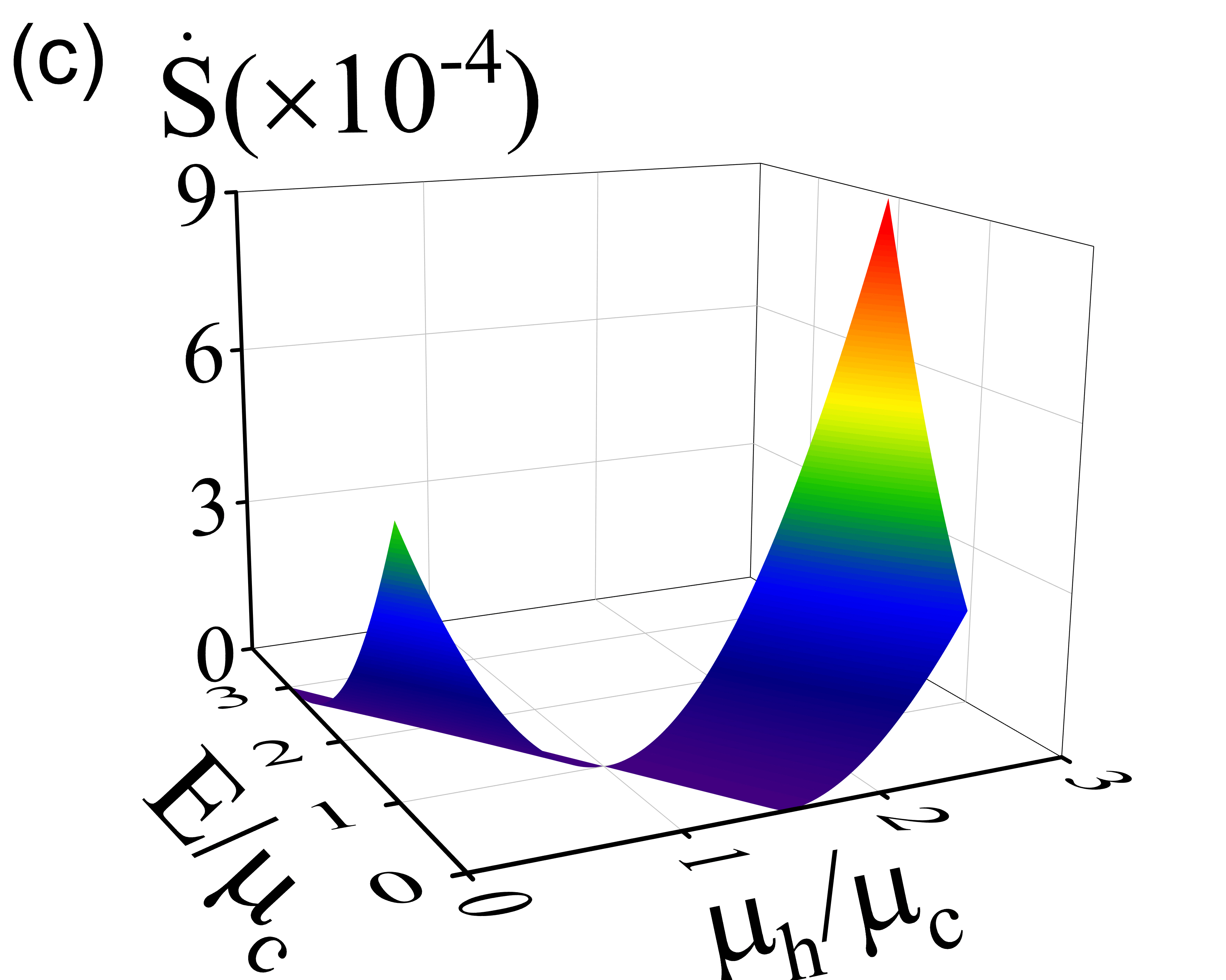
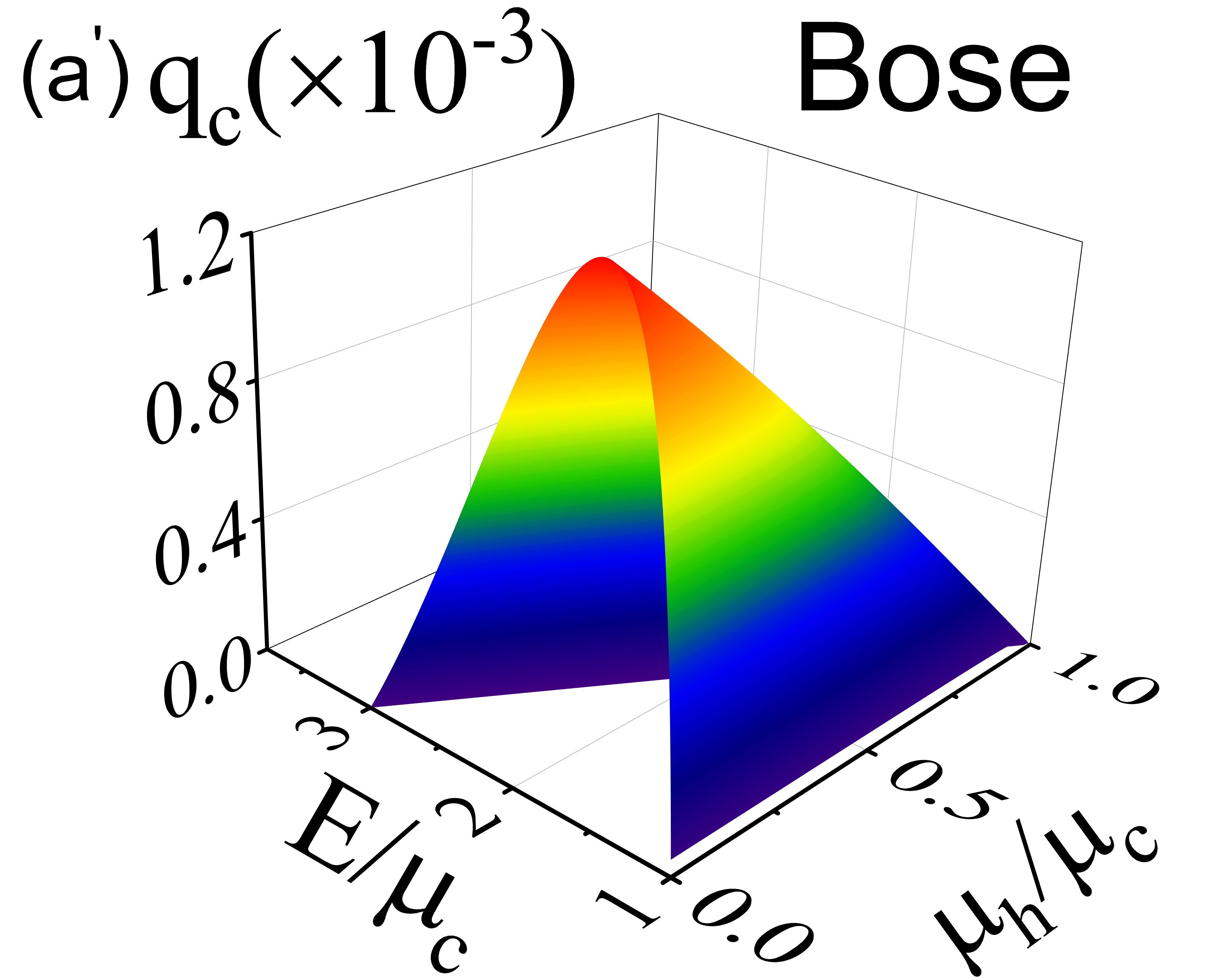
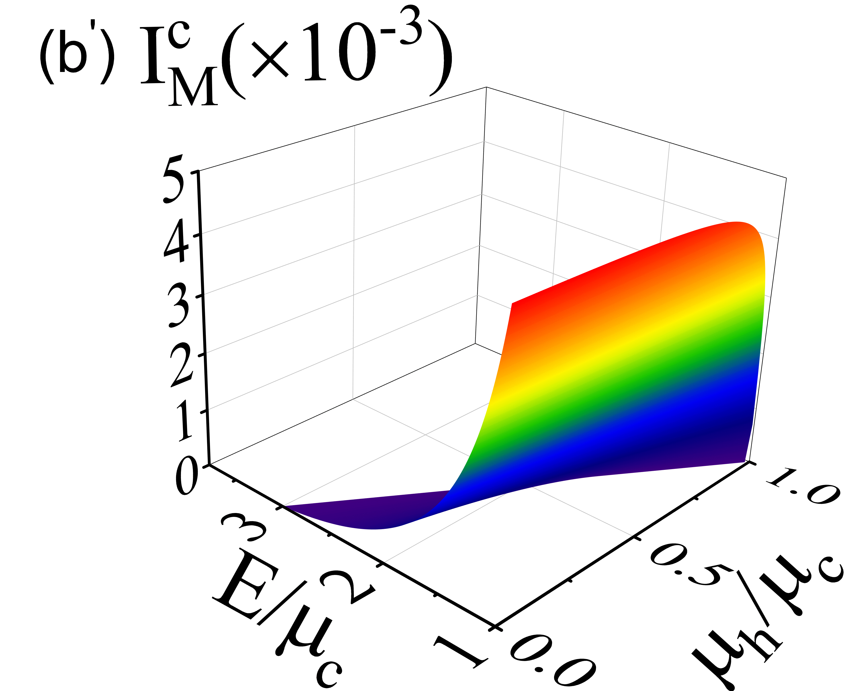
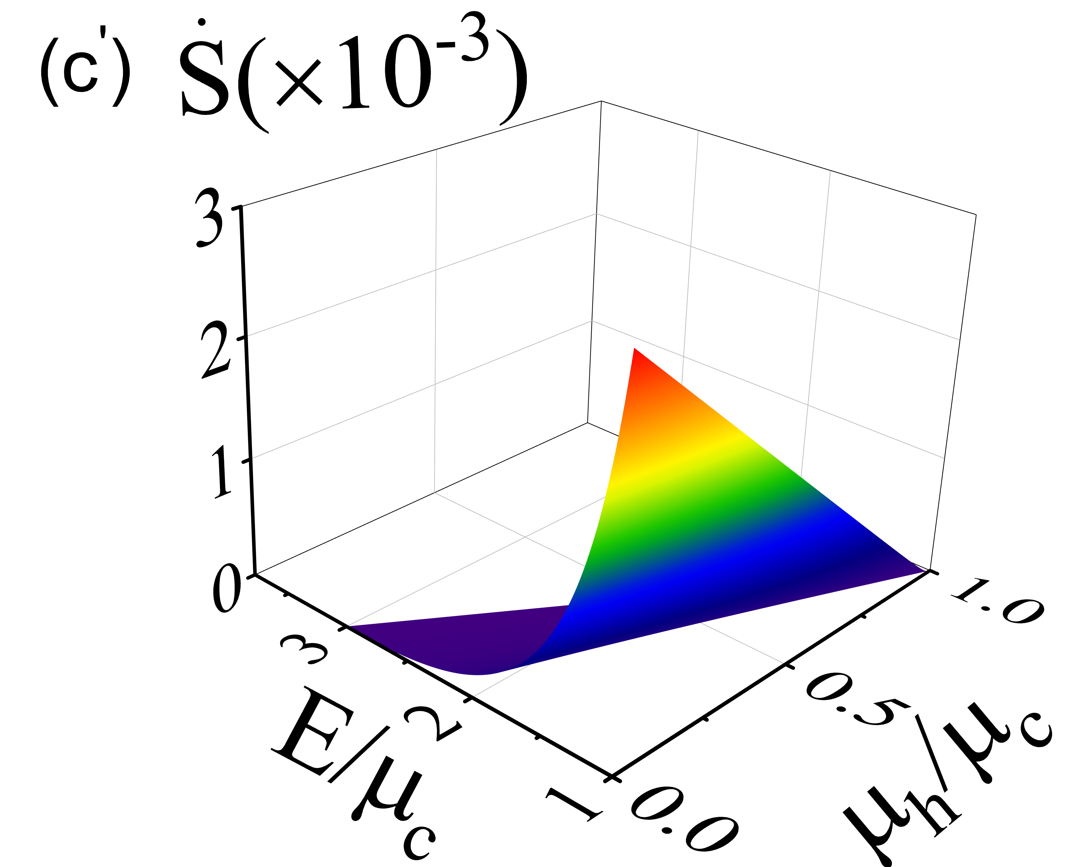
Figure 4: Three-dimension graphs of ($a$) [($a^{\prime}$)] the heat flow $q_{c}$, ($b$) [($b^{\prime}$)] particle current $I_{M}^{c}$, and ($c$) [($c^{\prime}$)] entropy production rate $\dot{S}$ of the QD device operating between two Fermi (Bose) reservoirs as functions of $E/\mu_{c}$ and $\mu_{h}/\mu_{c}$. The parameters $\mu_{c}=1.9$, $T_{h}=3$, $T_{c}=2$, and $\Gamma_{h}=\Gamma_{c}=0.01$.

For two reservoirs described by the Bose-Einstein distribution function, Eqs. (4)-(6) can be also used to generate the three dimensional graphs of the heat flow $q_{c}$, particle current $I_{M}^{c}$, and rate of entropy production $\dot{S}$ varying with $E/\mu_{c}$ and $\mu_{h}/\mu_{c}$, as shown in Figs. 4($a^{\prime}$)-($c^{\prime}$), respectively. It is found from Figs. 4($a^{\prime}$)-($c^{\prime}$) that only in the region of $\mu_{h}/\mu_{c}<1<E/\mu_{c}<E_{0}/\mu_{c}$, can the device have a non-zero reverse flow of heat. Because the distribution functions in reservoirs cannot be negative, there does not exist the region of the reverse heat flow for $\mu_{h}>\mu_{c}$ when two reservoirs are described by the Bose-Einstein distribution function. Thus, the QD coupled with Bose reservoirs can work only in region I as a device with a non-zero reverse flow of heat.

It is seen clearly from Fig. 4 that for the parameter values given by reservoirs, the heat flow $q_{c}$ is not a monotonic function of the energy level $E$ of the QD. When the optimal value of the energy level $E$ is chosen, i.e., $E/\mu_{c}=(E/\mu_{c})_{opt}$, the heat flow $q_{c}$ attains its maximum, as indicated by Figs. 5($a$) [$(a^{\prime})$] for the QD device operating between two Fermi (Bose) reservoirs. It is observed from Figs. 5($a$) [($a^{\prime}$)] that the maximum heat flow $q_{c,max}$ is a monotonically decreasing function of $\mu_{h}/\mu_{c}$ in the region of $\mu_{h}/\mu_{c}<1$, while it is a monotonically increasing function of $\mu_{h}/\mu_{c}$ in the region of $\mu_{h}/\mu_{c}>1$. $(E/\mu_{c})_{opt}$ is a monotonically decreasing function of $\mu_{h}/\mu_{c}$. The condition of the model availability requires $E>0$ so that $(E/\mu_{c})_{opt}$ has to be larger than zero. When $(E/\mu_{c})_{opt}=0$, $\mu_{h}/\mu_{c}=(\mu_{h}/\mu_{c})_{up}$, which is the upper bound of the ratio of two chemical potentials. When $\mu_{h}/\mu_{c}\geq(\mu_{h}/\mu_{c})_{up}$, $(E/\mu_{c})_{opt}\leq 0$ and the device can not have a reverse heat flow. Thus, $\mu_{h}/\mu_{c}=(\mu_{h}/\mu_{c})_{up}$ determines the right margin of region II in Fig. 3.

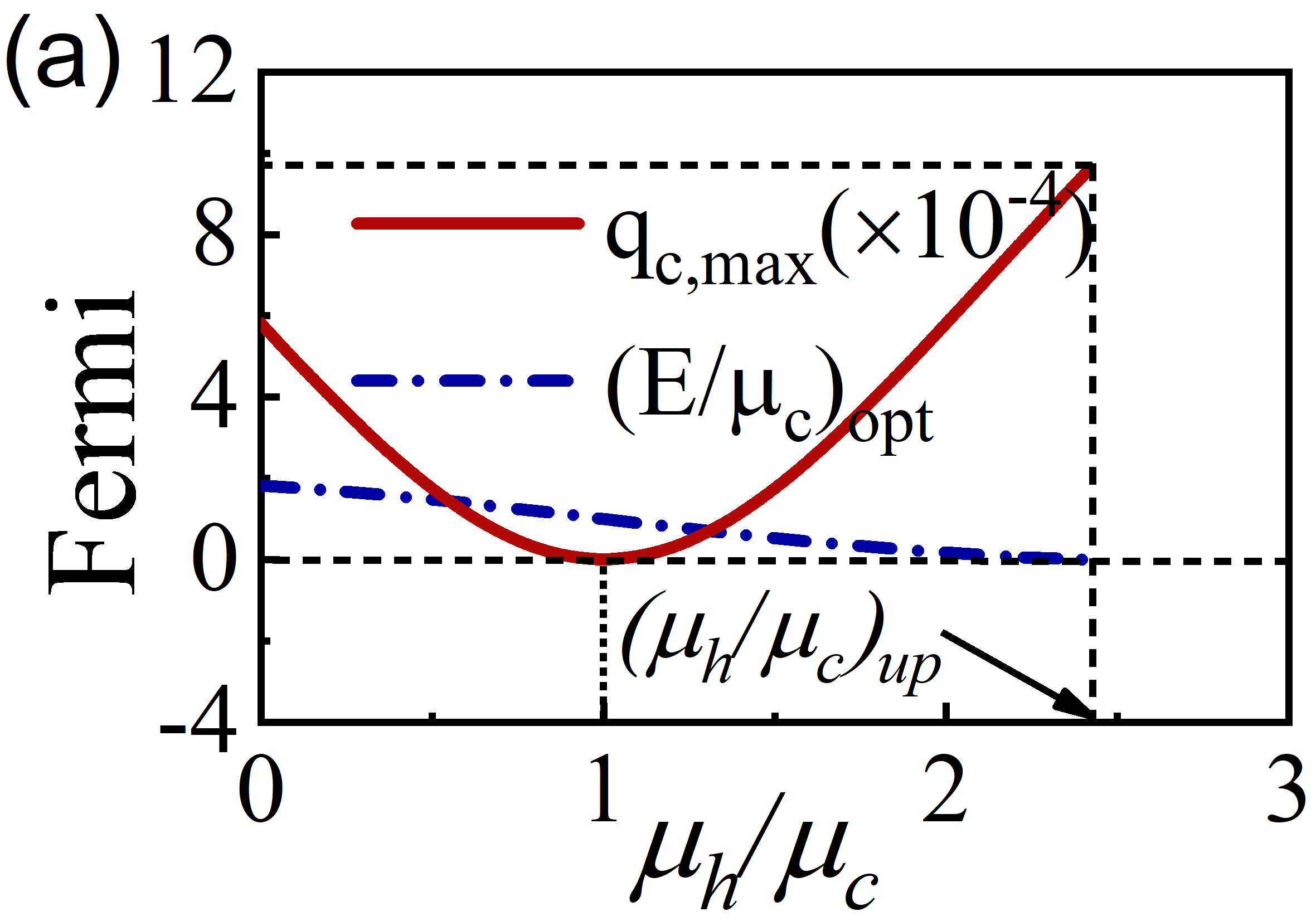
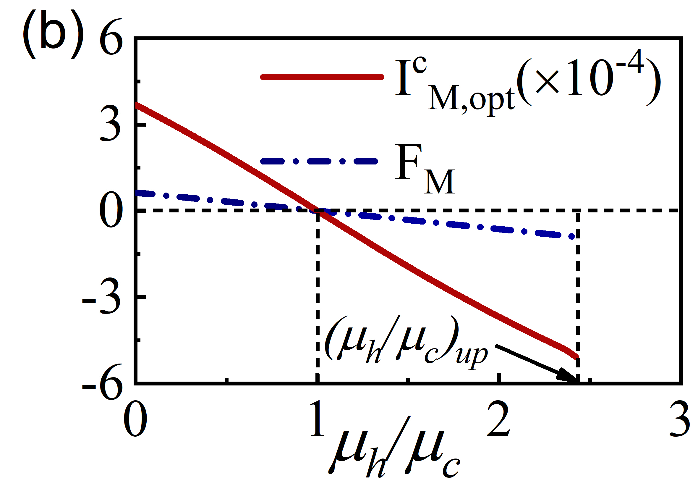
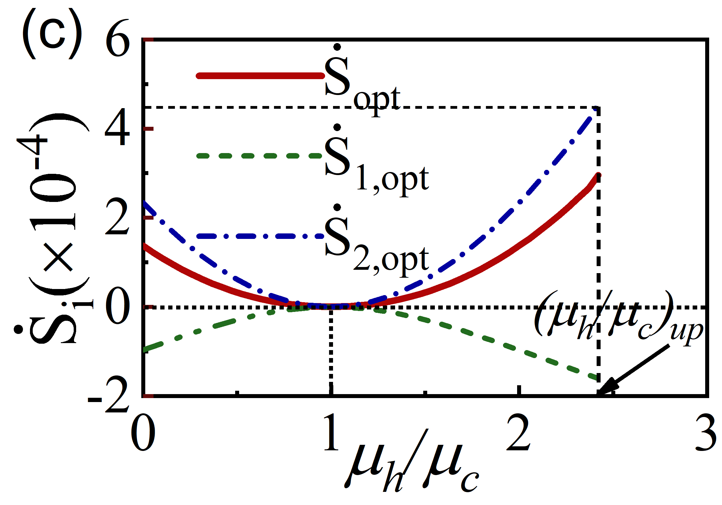
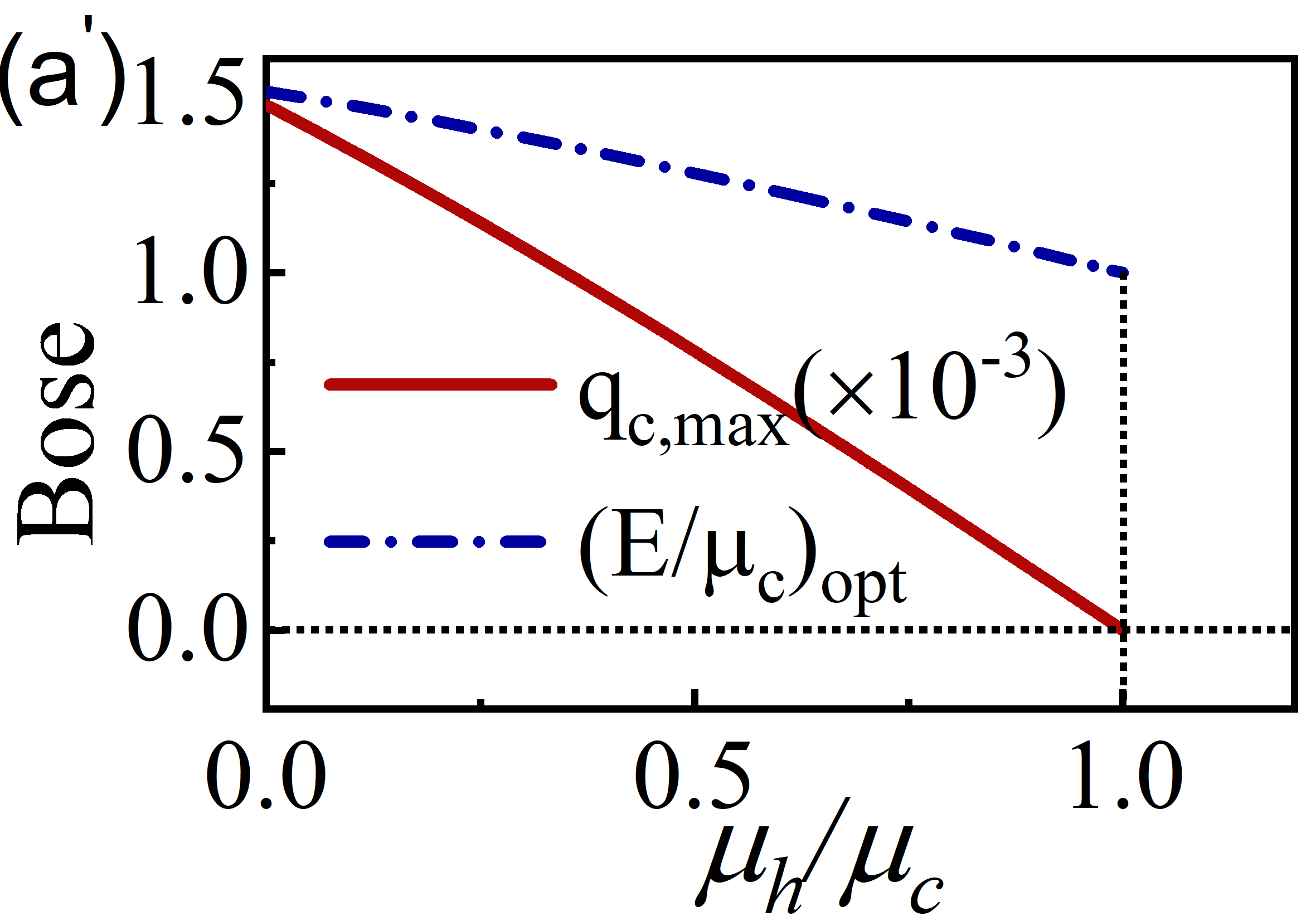
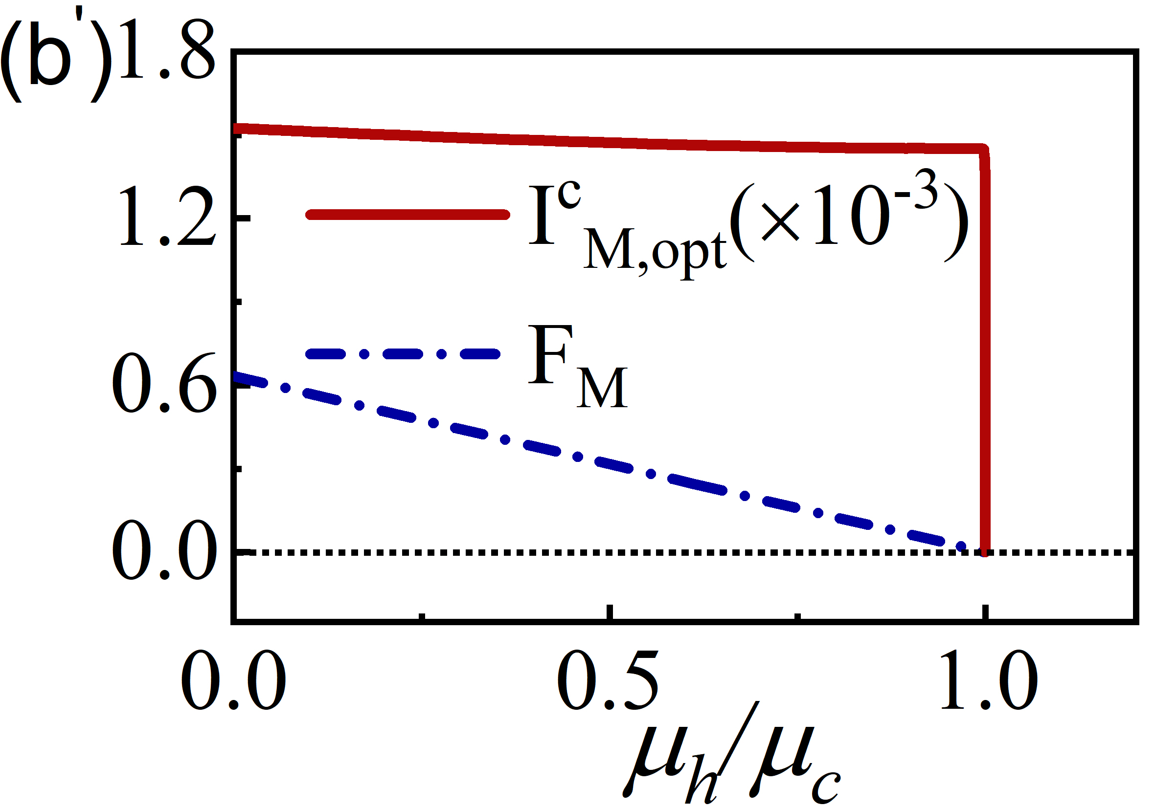
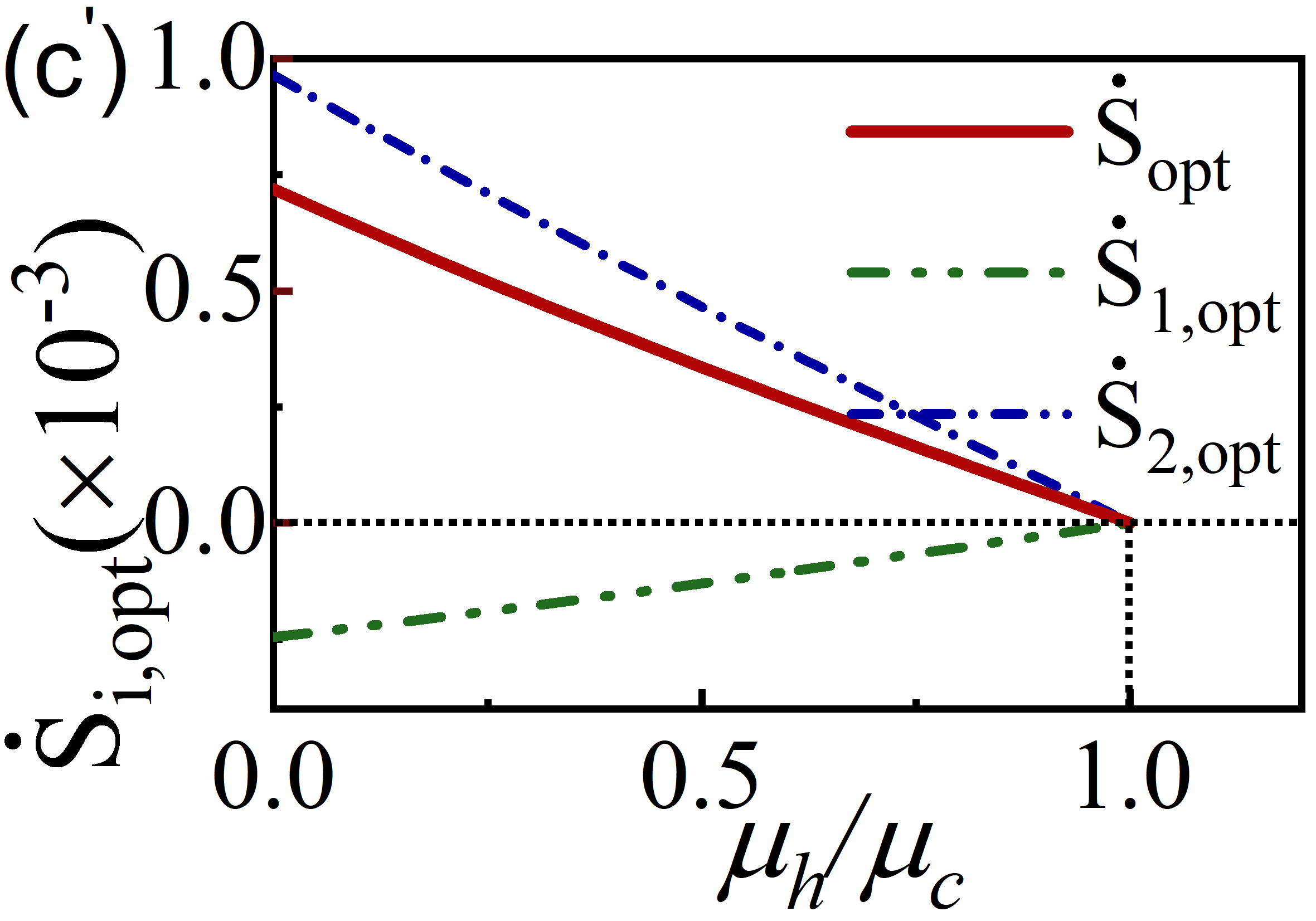
Figure 5: ($a$) [($a^{\prime}$)] The maximum heat flow $q_{c,max}$ and the optimized energy level $(E/\mu_{c})_{opt}$, ($b$) [($b^{\prime}$)] the optimized particle current $I_{M,opt}^{c}$ and $F_{M}$, and ($c$) [($c^{\prime}$)] the optimized entropy production rate $\dot{S}_{i,opt},$ $(\dot{S}_{opt},\dot{S}_{1,opt},\dot{S}_{2,opt},)$ of the QD device operating between two Fermi [Bose] reservoirs as functions of $\mu_{h}/\mu_{c}$. The parameters $\mu_{c}=1.9$, $T_{h}=3$, $T_{c}=2$, and $\Gamma_{h}=\Gamma_{c}=0.01$.

It is very interesting to note that the device in Fig. 1 has non-zero reverse heat flows without externally driving force. This result does not violate the second law of thermodynamics. The physical cause may be explained as follows: In the system shown in Fig. 1, besides the temperature difference, there exists another thermodynamic force resulting from the chemical potential difference, which can be defined as $F_{M}=(\mu_{c}-\mu_{h})/T_{h}$. This force is just the driving force of the reverse heat flow. In order to further expound this problem, the rate of entropy production may be rewritten as

$$\dot{S}=F_{T}q_{c}+F_{M}I_{M}^{c}=\dot{S}_{1}+\dot{S}_{2},$$ (8)

where $\dot{S}_{1}=F_{T}q_{c}$ is the rate of entropy production caused by the heat flow $q_{c}$, $F_{T}=1/T_{h}-1/T_{c}<0$ so that $\dot{S}_{1}\leq 0$, and $\dot{S}_{2}=F_{M}I_{M}^{c}$ is the rate of entropy production caused by particle current. Using Eqs. (4), (5), and (8), one can plot curves of the optimal values $I_{M,opt}^{c}$, $\dot{S}_{opt}$, $\dot{S}_{1,opt}$, and $\dot{S}_{2,opt}$ of $I_{M}^{c}$, $\dot{S}$, $\dot{S}_{1}$, and $\dot{S}_{2}$ at the maximum heat flow varying with $\mu_{h}/\mu_{c}$, as indicated by Figs. 5($b$) [($b^{\prime}$)] and ($c$) [($c^{\prime}$)] for the QD device operating between two Fermi (Bose) reservoirs, where the $\mu_{h}/\mu_{c}\sim F_{M}$ curves are also given in Figs. 5($b$) [($b^{\prime}$)]. It is seen from Figs. 5($b$) [($b^{\prime}$)] that the positive or negative values of $I_{M,opt}^{c}$ directly depend on that of $F_{M}$, so that $\dot{S}_{2}\geq 0$. $I_{M,opt}^{c}$ is proportional to $F_{M},$ and both $I_{M,opt}^{c}$ and $F_{M}$ are of monotonically decreasing functions of $\mu_{h}/\mu_{c}$. When $\mu_{h}/\mu_{c}=1$, both $I_{M,opt}^{c}$ and $F_{M}$ are equal to zero. It is observed from Figs. 5($c$) [($c^{\prime}$)] that $\dot{S}\geq 0$ because $\dot{S}_{2}\geq|\dot{S}_{1}|$. It shows once again that this seemingly paradoxical phenomenon appearing in the QD device does not violate the second law of thermodynamics.

It is seen from Fig. 5 that in the region of $\mu_{h}/\mu_{c}>1$, the heat flow $q_{c}$ of the QD device operating between two Fermi reservoirs attains its maximum when $\mu_{h}/\mu_{c}\rightarrow(\mu_{h}/\mu_{c})_{up}$; while in the region of $\mu_{h}/\mu_{c}<1$, the heat flow of the QD device obtains its maximum when $\mu_{h}/\mu_{c}=0$, and the maximum heat flow of the QD device operating between two Bose reservoirs is larger than that operating between two Fermi reservoirs

Using Eqs. (4) and (5), we can also plot the three-dimension graphs of another heat flow $q_{h}$ of the single QD device operating between two Fermi (Bose) reservoirs varying with $E/\mu_{c}$ and $\mu_{h}/\mu_{c}$, as shown in Fig. 6($a$) [($a^{\prime}$)]. It is observed from Fig. 6 that in regions I and II shown in Fig. 3, $q_{h}>q_{c}$. This implies the fact that the heat flow is amplified in the reverse transfer process of heat. It is seen from Eq. (5) that in the reverse transfer process of heat, the increment of heat is caused by the reduction of particle energy flow. It indicates that the amplification of heat does not violate the first law of thermodynamics. If defining an amplification coefficient as $\gamma=q_{h}/q_{c}$, one can plot the three-dimension graphs of the amplification coefficient $\gamma$ of the single QD device operating between two Fermi ( Bose) reservoirs varying with $E/\mu_{c}$ and $\mu_{h}/\mu_{c}$, as shown in Fig. 6($b$) [($b^{\prime}$)]. It can be observed that when $E=E_{0}$, $q_{c}=0$, $q_{h}=0$, and $\gamma=T_{h}/T_{c}>1$. When $E=\mu_{c}\neq\mu_{h}$, $\gamma\rightarrow\infty$. In regions I and II shown in Fig. 3, $q_{h}>q_{c}$ and $\gamma>T_{h}/T_{c}$.

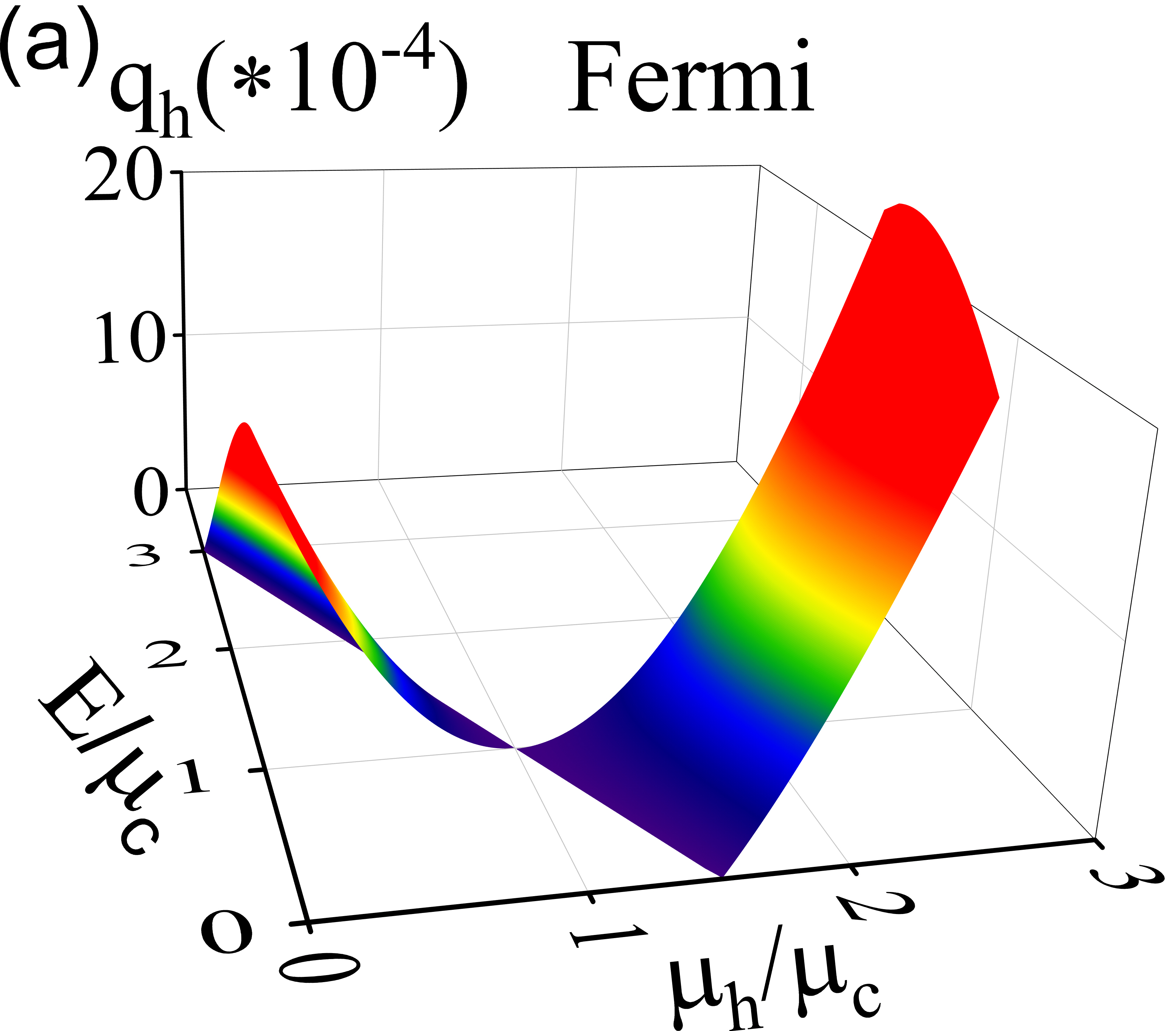
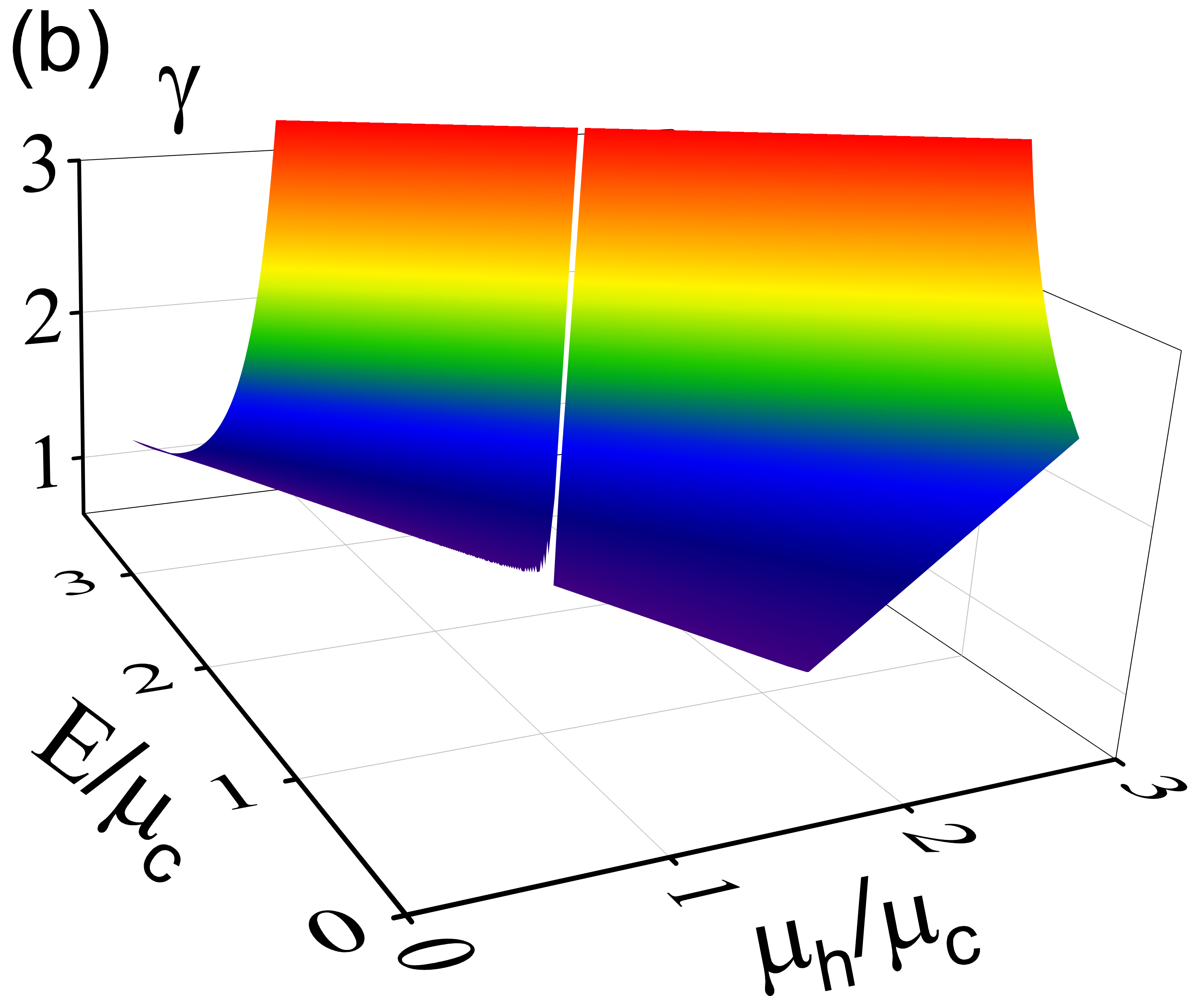
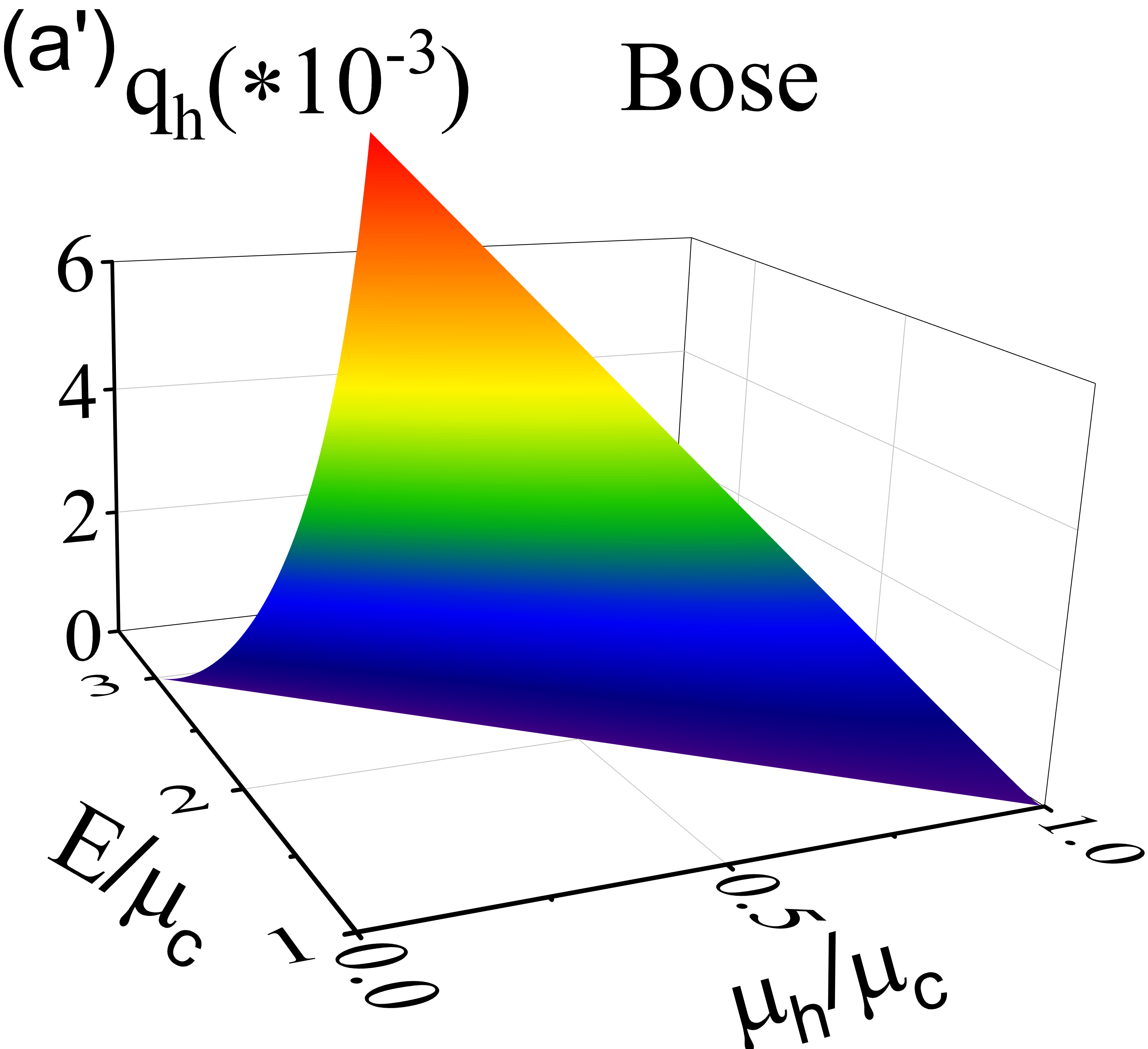
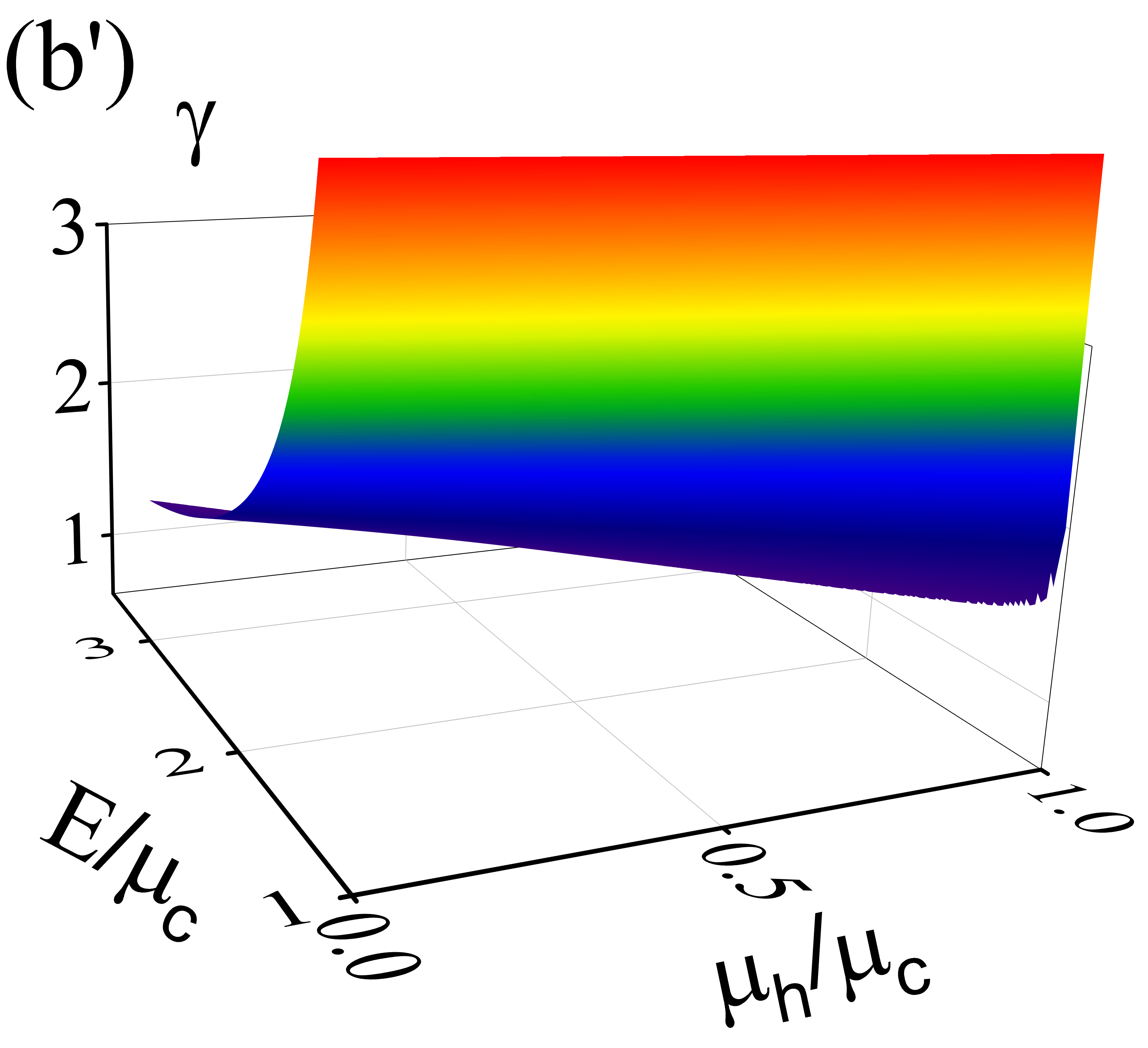
Figure 6: Three-dimension graphs of ($a$) [($a^{\prime}$)] the other heat flow $q_{h}$, ($b$) [($b^{\prime}$)] the amplification coefficient $\gamma$ of the QD device operating between two Fermi (Bose) reservoirs as functions of $E/\mu_{c}$ and $\mu_{h}/\mu_{c}$. The parameters $\mu_{c}=1.9$, $T_{h}=3$, $T_{c}=2$, and $\Gamma_{h}=\Gamma_{c}=0.01$.

IV An instance of the QD device

It is note worthy that the QD device can work as a micro/nano cooler because heat can be extracted from the cold reservoir. Using Eq. (5), one can calculate the coefficient of performance of the QD cooler as

$$\varepsilon=q_{c}/(q_{h}-q_{c})=\frac{E/\mu_{c}-1}{1-\mu_{h}/\mu_{c}}.$$ (9)

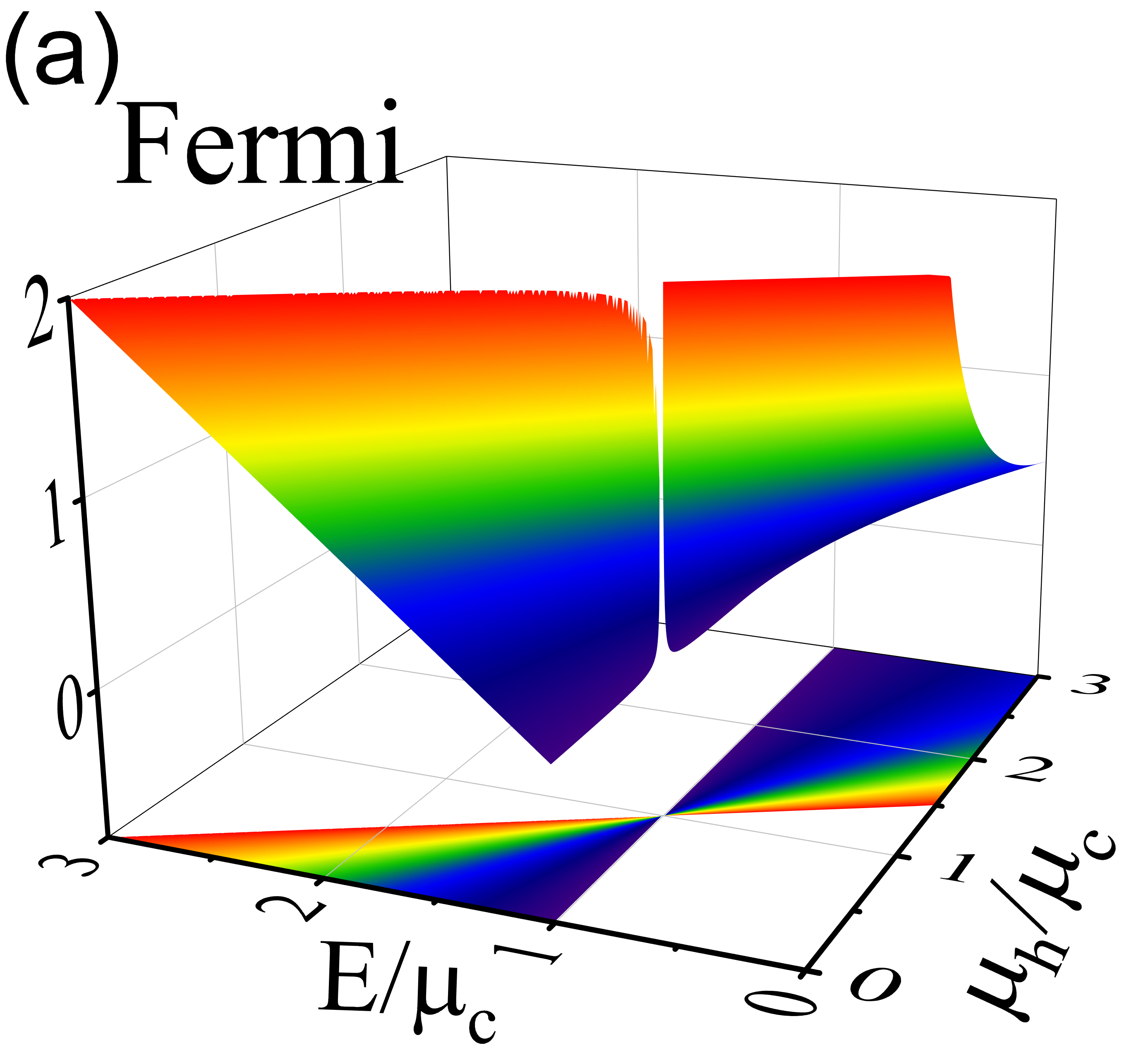
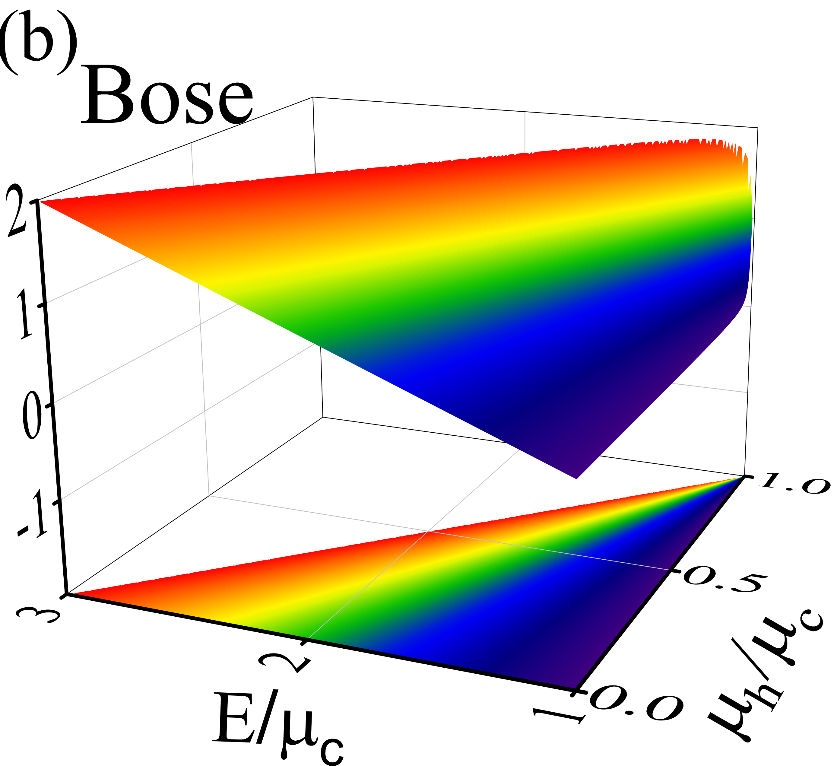
Figure 7: Three-dimension graphs of ($a$) [($b$)] the coefficient of performance $\varepsilon$ of the QD cooler operating between two Fermi (Bose) reservoirs as functions of $E/\mu_{c}$ and $\mu_{h}/\mu_{c}$. The parameters $\mu_{c}=1.9$, $T_{h}=3$, $T_{c}=2$, and $\Gamma_{h}=\Gamma_{c}=0.01$.

Equation (9) indicates that in region I shown in Fig. 3, $\varepsilon$ increases monotonically with the increase of $E/\mu_{c}$ and $\mu_{h}/\mu_{c}$; while in region II shown in Fig. 3, $\varepsilon$ decreases monotonically with the increase of $E/\mu_{c}$ and $\mu_{h}/\mu_{c}$; as illustrated in Fig. 7. In order to see the change trend of $\varepsilon$ more clearly, the projection graphs of $\varepsilon$ are also plotted in Fig. 7. When $E=E_{0}$, $q_{c}=0$ and $\varepsilon=T_{c}/(T_{h}-T_{c})\equiv\varepsilon_{r}$, which is the reversible coefficient of performance of the Carnot refrigerator operating between the two heat reservoirs at temperatures $T_{h}$ and $T_{c}$. When $E=\mu_{c}\neq\mu_{h}$, $q_{c}=0$ and $\varepsilon=0$. In regions I and II shown in Fig. 3, $q_{c}>0$ and $0<\varepsilon<\varepsilon_{r}$.

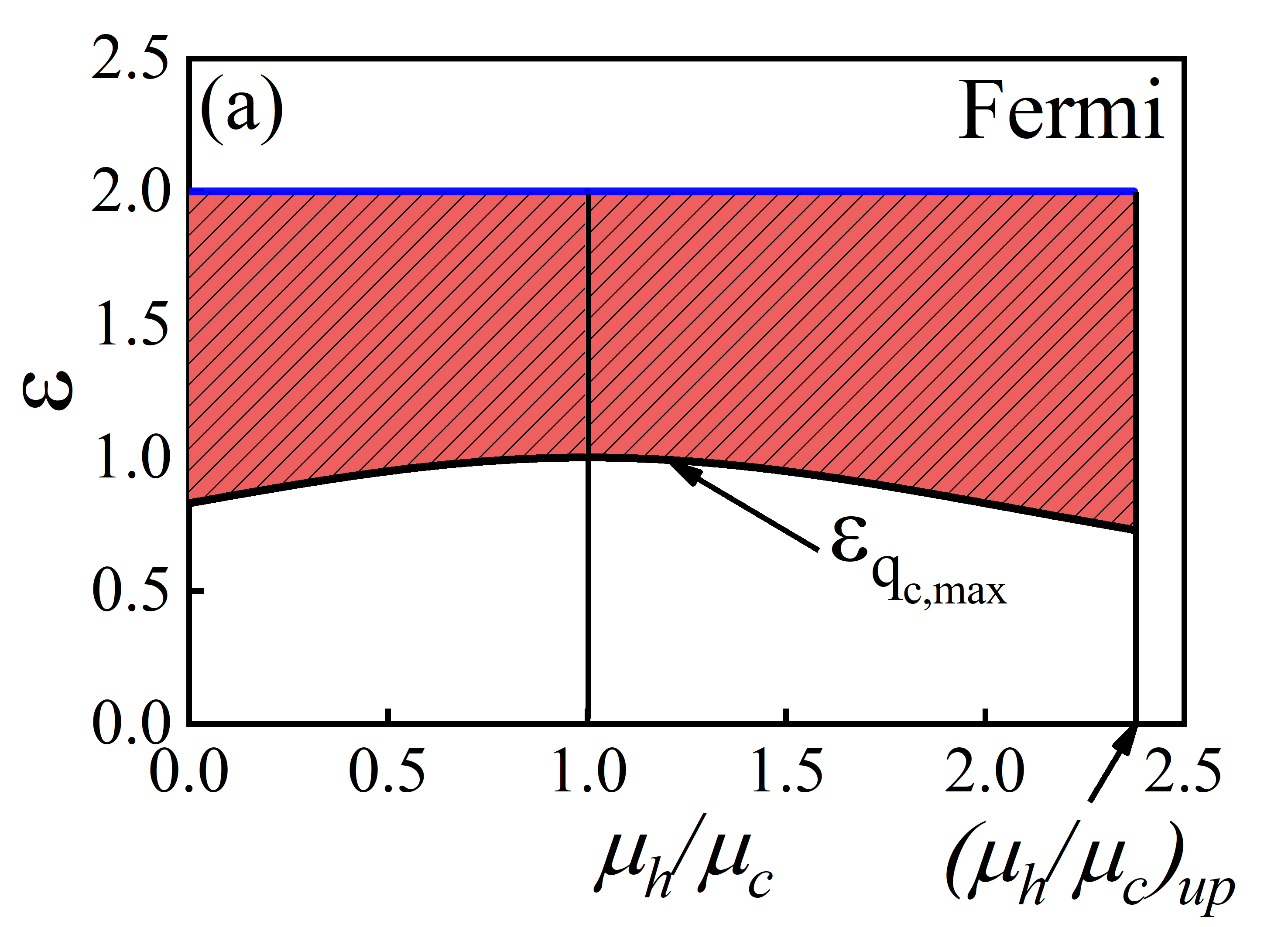
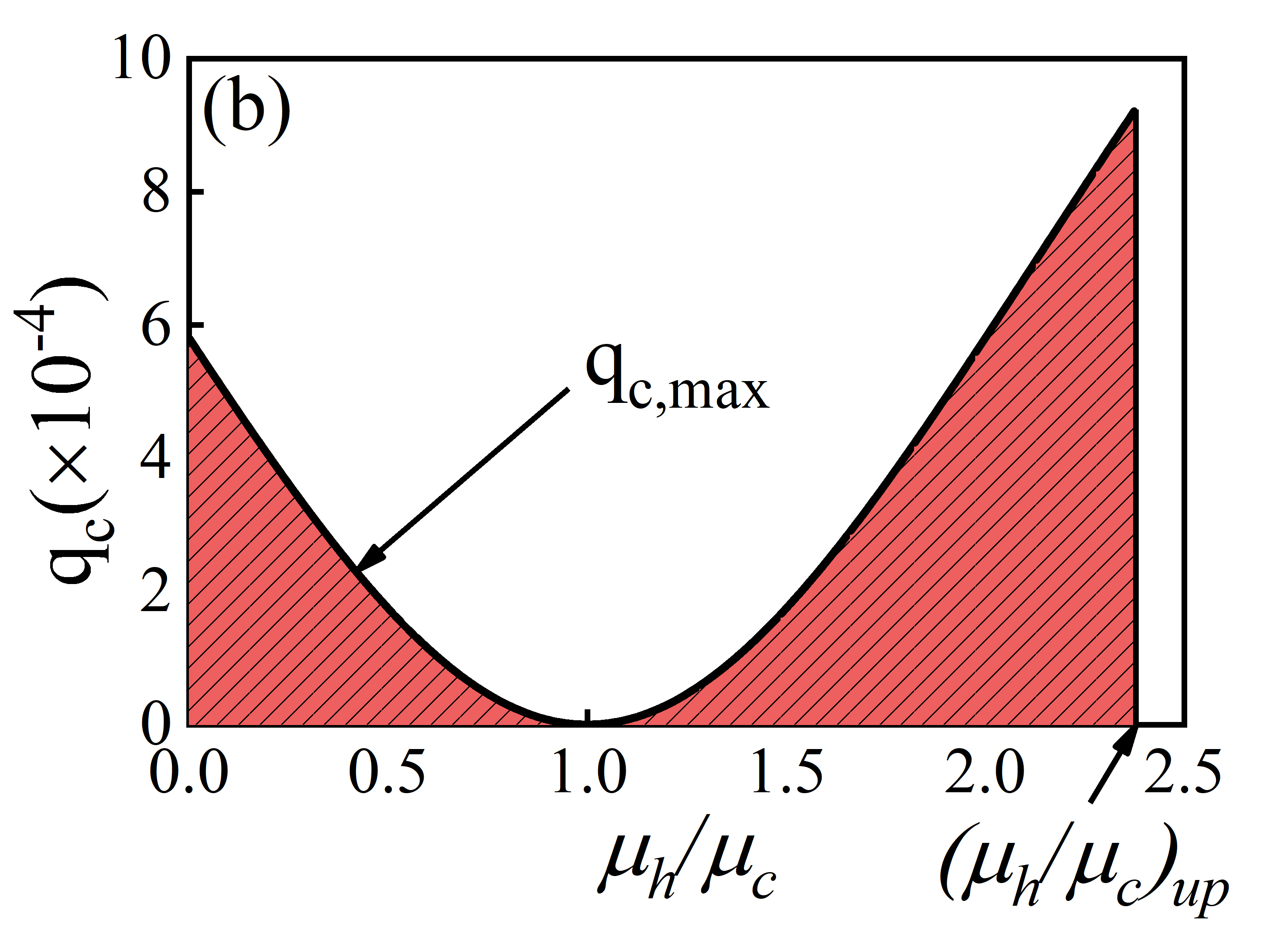
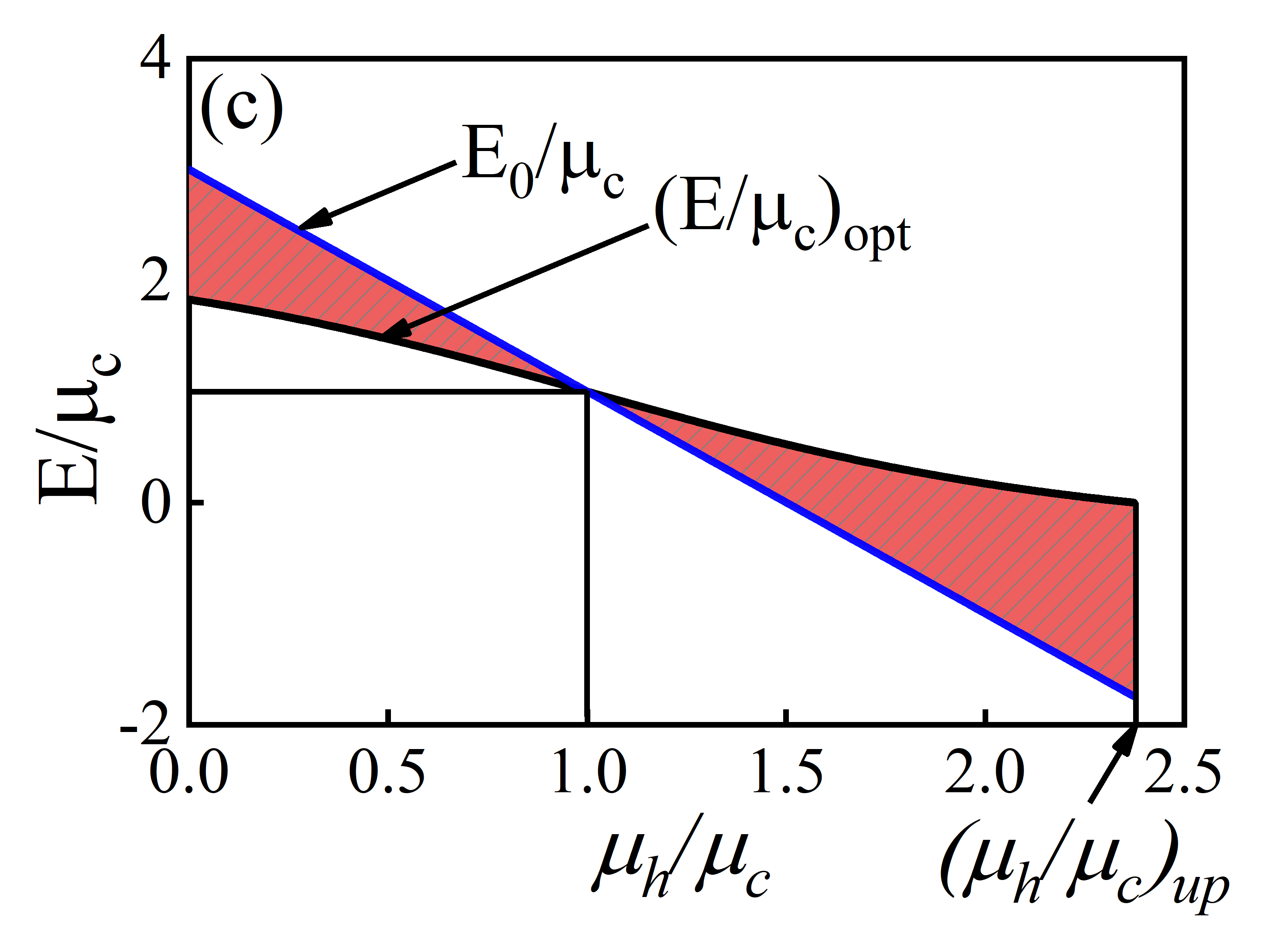
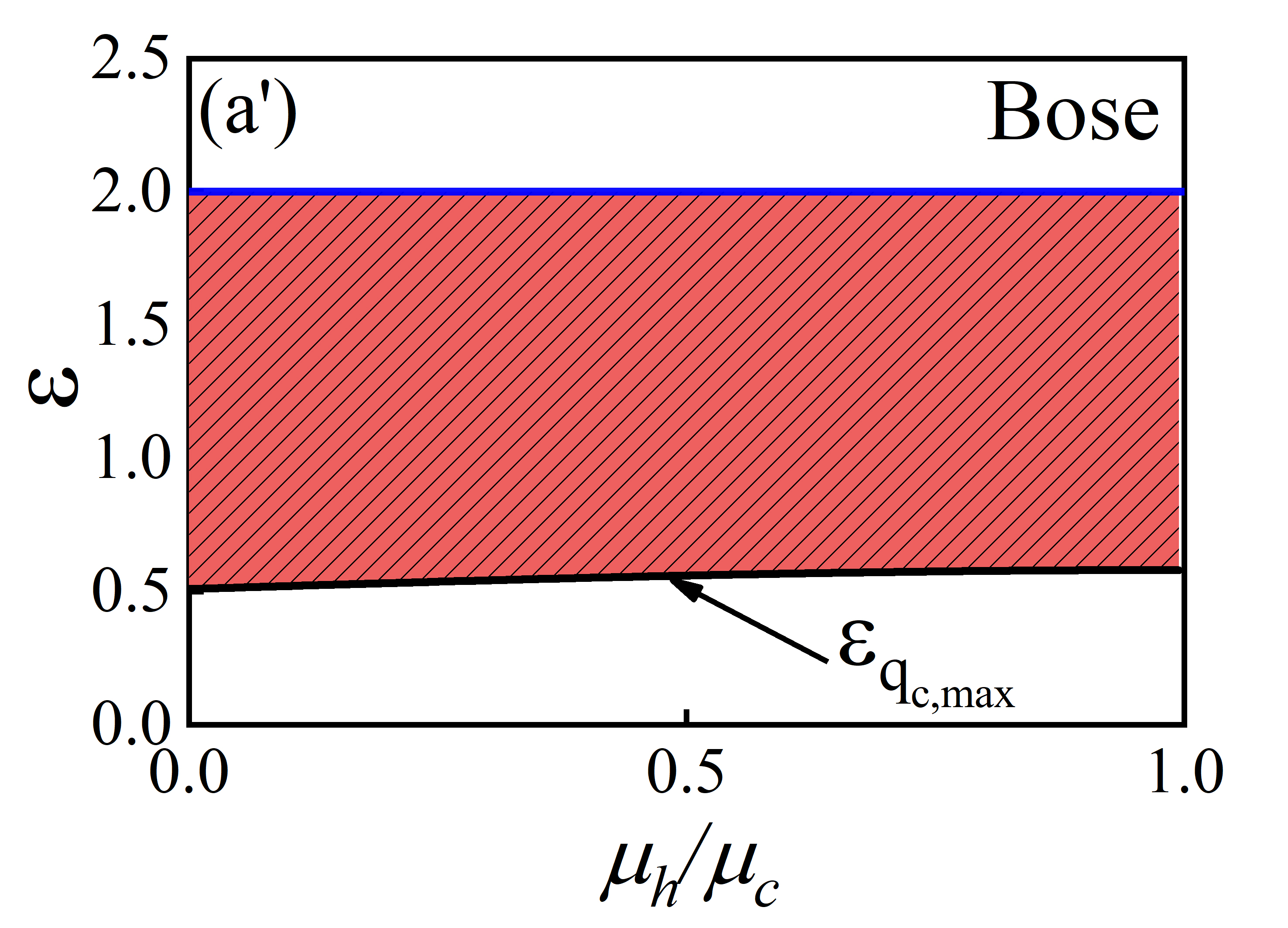
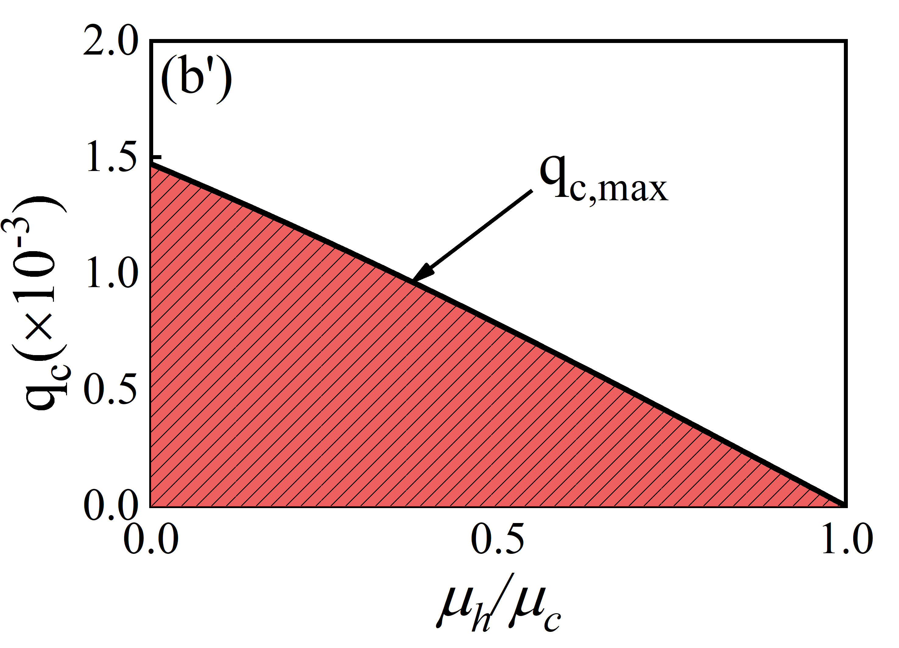
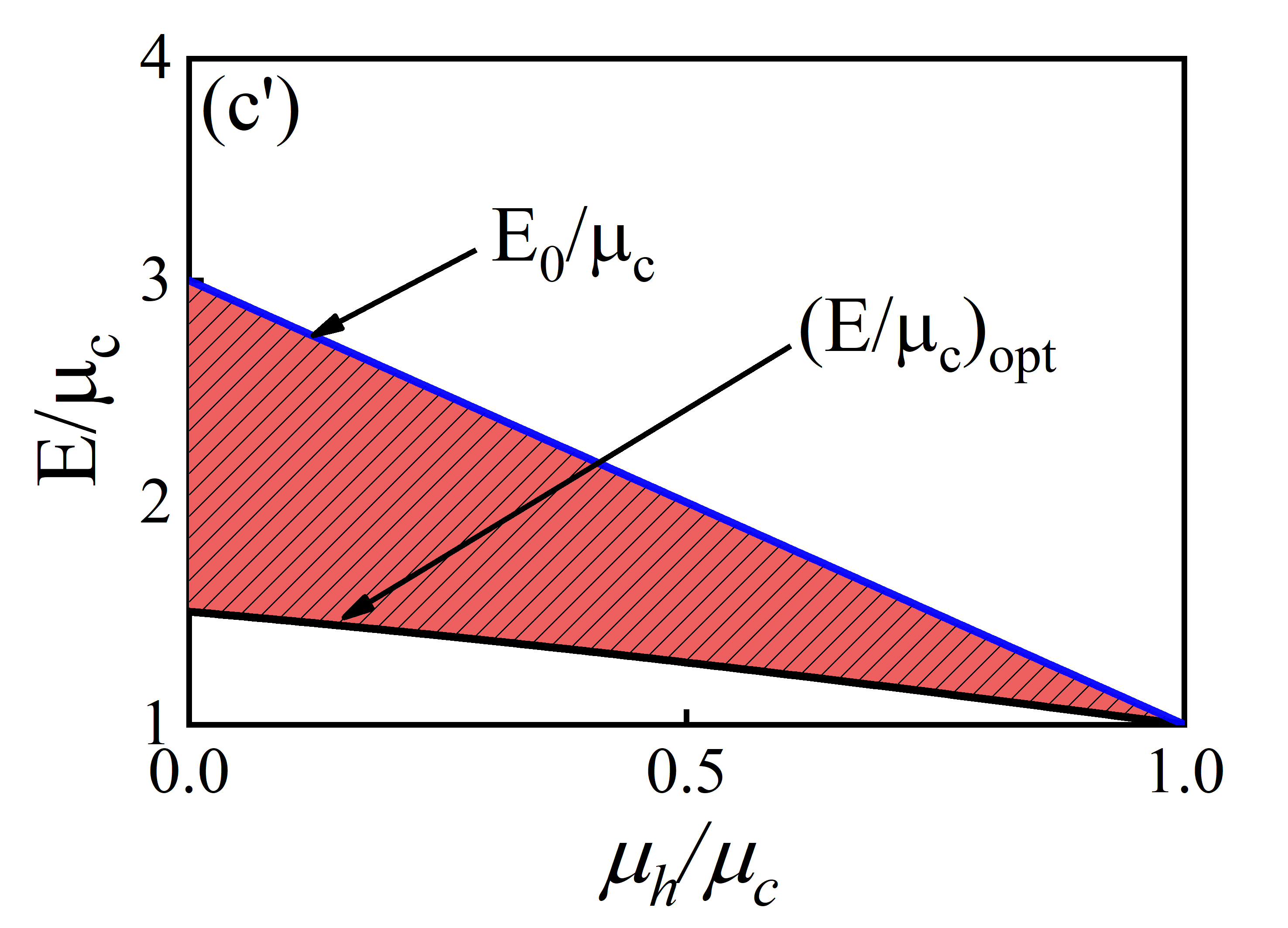
Figure 8: The optimum regions of ($a$) [($a^{\prime}$)] the coefficient of performance $\varepsilon$, ($b$) [($b^{\prime}$)] the cooling rate $q_{c}$, and ($c$) [($c^{\prime}$)] the energy level $E/\mu_{c}$ of the QD cooler operating between two Fermi [Bose] reservoirs for differently given values of $\mu_{h}/\mu_{c}$. The parameters $\mu_{c}=1.9$, $T_{h}=3$, $T_{c}=2$, and $\Gamma_{h}=\Gamma_{c}=0.01$.

For a micro/nano cooler, one always wants to obtain a coefficient of performance and a cooling rate as large as possible. According to Figs. 4 and 7, we can further determine the optimum regions of $\varepsilon$, $q_{c}$ and $E/\mu_{c}$, as shown in Fig. 8. Form Fig. 8, we can obtain the optimum selection criteria of the key parameters of the QD cooler as

$$\begin{cases}\begin{array}[]{c}\varepsilon_{r}>\varepsilon\geq\varepsilon_{q_{c,max}}\\ 0<q_{c}\geq q_{c,max}\\ E_{0}/\mu_{c}>E/\mu_{c}\geq(E/\mu_{c})_{opt}\\ E_{0}/\mu_{c}<E/\mu_{c}\leq(E/\mu_{c})_{opt}\end{array}&\begin{array}[]{c}\\ \\ (\mu_{h}/\mu_{c}<1),\\ (\mu_{h}/\mu_{c}>1)\end{array}\end{cases}$$ (10)

where $\varepsilon_{q_{c,max}}$ is the coefficient of performance of the QD cooler at the maximum cooling rate $q_{c,max}$. Equation (10) may provide some guidance for the experiment and development of real micro/nano coolers.

V conclusions

It has been proved that the single QD embedded between the two reservoirs described by different statistical distribution functions can realize the reverse flow and amplification of heat without externally driving force and this seemingly paradoxical phenomenon does not violate the laws of thermodynamics. It has been pointed out that the QD device can work as a micro/nano cooler. The performance characteristics of the cooler were revealed. The optimum operation regions of the cooler were determined and the selection criteria of key parameters were provided. The results obtained show that the proposed model has not only guiding significance for the theoretical investigation of quantum devices but also potential value for the practical application of micro/nano devices.

- (1) C. W. Chang, D. Okawa, A. Majumdar, and A. Zettl, Solid-state thermal rectifier, Science 314, 1121-1124 (2006).
- (2) P. Ben-Abdallah and S. A. Biehs, Near-field thermal transistor, Phys. Rev. Lett. 112, 044301 (2014).
- (3) K. Joulain, J. Drevillon, Y. Ezzahri, and J. Ordonez-Miranda, Quantum thermal transistor, Phys. Rev. Lett. 116, 200601 (2016).
- (4) C. N. Murphy and P. R. Eastham, Quantum control of excitons for reversible heat transfer, Commun. Phys. 2, 1-8 (2019).
- (5) P. Ben-Abdallah and S. A. Biehs, Phase-change radiative thermal diode, Appl. Phys. Lett. 103, 191907 (2013).
- (6) Y. Li, X. Shen, Z. Wu, J. Huang, Y. Chen, Y. Ni, and J. Huang, Temperature-dependent transformation thermotics: from switchable thermal cloaks to macroscopic thermal diode, Phys. Rev. Lett. 115, 195503 (2015).
- (7) M. Y. Wong, C. Y. Tso, T. C. Ho, and H. H. Lee, A review of state of the art thermal diodes and their potential applications, Int. J. Heat Mass Transf. 164, 120607 (2019).
- (8) G. Wehmeyer, T. Yabuki, C. Monachon, J. Wu, and C. Dames, Thermal diodes, regulators, and switches: physical mechanisms and potential applications, Appl. Phys. Rev. 4, 041304 (2017).
- (9) D. Prete, P. A. Erdman, V. Demontis, V. Zannier, D. Ercolani, L. Sorba, F. Beltram, F. Rossella, F. Taddei, and S. Roddaro, Thermoelectric conversion at 30 K in InAs/InP nanowire quantum dots, Nano lett. 19, 3033-3039 (2019).
- (10) R. Rafeek and D. Mondal, Noise-induced symmetry breaking of self-regulators: nonequilibrium transition toward homochirality, J. Chem. Phys. 154, 244906 (2021).
- (11) B. Guo, T. Liu, and C. Yu, Multifunctional quantum thermal device utilizing three qubits, Phys. Rev. E 99, 032112 (2019).
- (12) S. S. Pidaparthi and C. S. Lent, Energy dissipation during two-state switching for quantum-dot cellular automata, J. Appl. Phys. 129, 024304 (2021).
- (13) A. Ott, Y. Hu, X. Wu, and S. Biehs, Radiative thermal switch exploiting hyperbolic surface phonon polaritons, Phys. Rev. Appl. 15, 064073 (2021).
- (14) H. L. Edwards, Q. Niu, and A. L. de Lozanne, A quantum-dot refrigerator, Appl. Phys. Lett. 63, 1815 (1993).
- (15) F. Chi, J. Zheng, Y. Liu, and Y. Guo, Refrigeration effect in a single-level quantum dot with thermal bias, Appl. Phys. Lett. 100, 233106 (2012).
- (16) S. Su, W. Shen, J. Du, and J. Chen, Thermodynamic coupling rule for quantum thermoelectric devices, J. Phys. D: Appl. Phys. 53, 095502 (2019).
- (17) M. Esposito, K. Lindenberg, and C. Van den Broeck, Thermoelectric efficiency at maximum power in a quantum dot, Europhys. Lett. 85, 60010 (2009).
- (18) M. Josefsson, A. Svilans, A. M. Burke, E. A. Hoffmann, S. Fahlvik, C. Thelander, M. Leijnse, and H. Linke, A quantum-dot heat engine operating close to the thermodynamic efficiency limits, Nat. Nanotechnol. 13, 920-924 (2018).
- (19) M. Josefsson, A. Svilans, H. Linke, and M. Leijnse, Optimal power and efficiency of single quantum dot heat engines: theory and experiment, Phys. Rev. B 99, 235432 (2019).
- (20) B. Dutta, D. Majidi, A. G. Corral, P. A. Erdman, S. Florens, T. A. Costi, H. Courtois, and C. B. Winkelmann, Direct probe of the Seebeck coefficient in a Kondo-correlated single-quantum-dot transistor, Nano Lett. 19, 506−511 (2018).
- (21) B. Dutta, D. Majidi, N. W. Talarico, N. L. Gullo, H. Courtois, and C. B. Winkelmann, Single-quantum-dot heat valve, Phys. Rev. Lett. 125, 237701 (2020).
- (22) Y. Zhang, Z. Yang, X. Zhang, B. Lin, G. Lin, and J. Chen, Coulomb-coupled quantum-dot thermal transistors, EPL 122, 17002 (2018).
- (23) Y. Zhang, X. Zhang, Z. Ye, G. Lin, and J. Chen, Three-terminal quantum-dot thermal management devices, Appl. Phys. Lett. 110, 153501 (2017).
- (24) G. Jaliel, R. K. Puddy, R. Sánchez, A. N. Jordan, B. Sothmann, I. Farrer, J. P. Griffiths, D. A. Ritchie, and C. G. Smith, Experimental realization of a quantum dot energy harvester, Phys. Rev. Lett. 123, 117701 (2019).
- (25) S. Dorsch, A. Svilans, M. Josefsson, B. Goldozian, M. Kumar, C. Thelander, A. Wacker, and A. Burke, Heat driven transport in serial double quantum dot devices, Nano letters, 21, 988-994 (2019).
- (26) G. Schaller, Open Quantum Systems Far from Equilibrium, Lecture Notes in Physics (Springer, New York, 2014).
- (27) S. Su, C. Sun, S. Li, and J. Chen, Photoelectric converters with quantum coherence, Phys. Rev. E 93, 052103 (2016).
- (28) D. Segal, Single mode heat rectifier: controlling energy flow between electronic conductors, Phys. Rev. Lett. 100, 105901 (2008).
- (29) M. F. O’Dwyer, R. A. Lewis, and C. Zhang, Electronic efficiency in nanostructured thermionic and thermoelectric devices, Phys. Rev. B 72, 205330 (2005).
- (30) S. Su, Y. Zhang, J. Chen, and T. M. Shih, Thermal electron-tunneling devices as coolers and amplifiers, Sci. Rep. 6, 21425 (2016).
- (31) T. E. Humphrey, R. Newbury, R. P. Taylor, and H. Linke, Reversible quantum Brownian heat engines for electrons, Phys. Rev. Lett. 89, 116801 (2002).
- (32) J. D. Barrow, The constants of nature: From alpha to omega-the numbers that encode the deepest secrets of the universe (Pantheon, New York, 2002).
- (33) J. Du, W. Shen, X. Zhang, S. Su, J. Chen, Quantum-dot heat engines with irreversible heat transfer, Phys. Rev. Res. 2, 013259 (2020).