Online Multi-horizon Transaction Metric Estimation with Multi-modal Learning in Payment Networks

Abstract.

Predicting metrics associated with entities’ transnational behavior within payment processing networks is essential for system monitoring. Multivariate time series, aggregated from the past transaction history, can provide valuable insights for such prediction. The general multivariate time series prediction problem has been well studied and applied across several domains, including manufacturing, medical, and entomology. However, new domain-related challenges associated with the data such as concept drift and multi-modality have surfaced in addition to the real-time requirements of handling the payment transaction data at scale. In this work, we study the problem of multivariate time series prediction for estimating transaction metrics associated with entities in the payment transaction database. We propose a model with five unique components to estimate the transaction metrics from multi-modality data. Four of these components capture interaction, temporal, scale, and shape perspectives, and the fifth component fuses these perspectives together. We also propose a hybrid offline/online training scheme to address concept drift in the data and fulfill the real-time requirements. Combining the estimation model with a graphical user interface, the prototype transaction metric estimation system has demonstrated its potential benefit as a tool for improving a payment processing company’s system monitoring capability.

1. Introduction

The main responsibility of a payment network company like Visa is facilitating transactions between different parties with reliability, convenience, and security. For this reason, it is crucial for a payment network company to actively study the transaction behavior of different entities (e.g., countries, card issuers, and merchants) in real-time because any unexpected disruption could impair users’ experience and trust towards the network. For example, an unexpected network outage could be detected promptly if a payment network company monitors the transaction volumes of different geographical regions (Mora, 2019). Fraudulent activities, such as the infamous ATM cash-out attack (Thomas, 2020), could be easily spotted if the abnormal decline rate¹ of the attacked card issuer is monitored. Additionally, it is possible to enhance the existing fraud detection system if the real-time fraud rate¹ of the associated merchant is estimated and supplied to the fraud detection system (Zhang et al., 2020). Other business services provided by payment network companies, like ATM management (Pearson, [n.d.]) and merchant attrition (Kapur et al., 2020), can also benefit from an effective monitoring system.

For monitoring purposes, we propose a real-time transaction metric estimation system that estimates the future transaction metrics of a given set of entities based on their historical transaction behaviors. Such estimation capability can help payment network companies’ monitoring effort in two ways: 1) we can detect abnormal events (e.g., payment network outage, ATM cash-out attack) by comparing the estimated transaction metric with the real observation, and introduce necessary interventions in time to prevent further loss, and 2) the online estimation provides instant access to transaction metrics (e.g., fraud rate¹) that are not immediately available due to the latency introduced from data processing, case investigation, and data verification.

We face the following three challenges when building the prototype transaction metric estimation system:

Challenge 1: Concept Drift. In payment networks, the transaction behaviors of entities are always evolving. A static prediction system will always become outdated when a sufficient amount of time has passed because of such incremental concept drift (Gama et al., 2014). Moreover, external factors like economy, geopolitics, and pandemic could abruptly change the transaction behaviors, subsequently causes a sudden concept drift (Gama et al., 2014) and degrades the quality of the prediction made by a static prediction system. Concept drift is an added layer of complexity in real-world production data often absent from cleaned experimental datasets.

Challenge 2: Multiple Modalities. Because many of the aforementioned applications require our system to estimate time-varying patterns within transaction metrics, we use multivariate time series to represent the dynamic aspect of transaction behaviors. However, recent work studying merchant behaviors using time series has demonstrated that time-series alone is not sufficient for making accurate predictions (Yeh et al., 2020c). Instead, a multi-modality approach that incorporates the relationship or interaction among merchants is preferred. Similar phenomena can be observed with other types of entities in the payment network. As shown in Figure 1(a), the time series of Australia and New Zealand exhibit similar trends, but due to the difference between their interaction vectors, their corresponding target transaction metrics have different patterns. For another country-pair of Hungary and the Czech Republic (see Figure 1(b)), since both time series and interaction vectors show similar patterns, the transaction metrics are identical too. In other words, additional modalities further distinguish countries with similar time series, and the system could use such information to better estimate the target country-specific transaction metric. Nevertheless, conventional approaches (Taieb and Atiya, 2015; Wen et al., 2017; Shih et al., 2019; Fan et al., 2019; Zhuang et al., 2020; Yeh et al., 2020b) lack the ability and means to utilize the additional modalities.

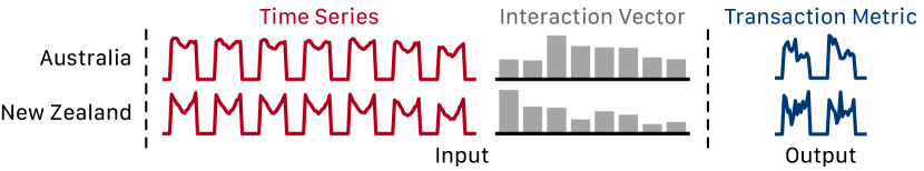
(a) Australia and New Zealand have similar time series features. However, due to the differences in interaction vector, the transaction metric prediction is different.

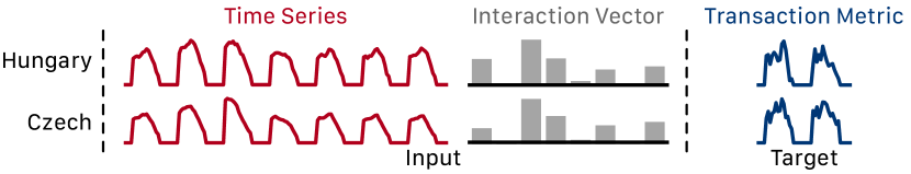
(b) Hungary and Czech have similar time series features and interaction vectors. As a result, the transaction metric prediction is similar as well.

Figure 1. Time series features and interaction vector feature are both essential for predicting transaction metric.

Challenge 3: Multiple Time-Step Predictions. With a significant amount of transactions in a system, running predictions for each time step is unrealistic due to the prohibitively high operation cost. A more realistic approach would be to predict multiple time-steps at once. This problem is known as multi-horizon time series prediction, and it requires a unique model design to handle such a situation. Merely applying a 1-step prediction model in a rolling fashion could lead to inferior results as the prediction for a later time-step is made based on estimated input. That is, errors from the earlier time-step would propagate to later time-steps (Taieb and Atiya, 2015; Wen et al., 2017).

We use online learning techniques to resolve challenges 1. Online learning is a supervised learning scheme that the training data is made available incrementally over time. Several notable works in online learning (Žliobaitė, 2010; Gama et al., 2014; Krawczyk et al., 2017; Hoi et al., 2018; Losing et al., 2018; Lu et al., 2018) have been published in recent years. Although the concept drift challenge is studied in these works, it is not well-tailored for transaction metric estimation using deep learning models. As a result, we have outlined and benchmarked a set of online learning strategies suitable for deep learning models and identify the best strategy for our prototype.

To tackle challenges 2 and 3, we design a deep learning model capable of estimating multi-horizon transaction metrics using multiple modalities. The proposed model has five unique components: interaction encoder, temporal encoder, scale decoder, shape decoder, and amalgamate layer. The interaction encoder is used to process the interaction modality, i.e., how entities interact with each other in our data. The temporal encoder dissects the temporal data and learns the inherent patterns. The scale and shape decoders provide two distinct yet related perspectives regarding the estimated multi-horizon transaction metric. Finally, an amalgamate layer fuses the outputs of scale and shape decoder to synthesize the output.

Our contributions include:

• We propose and benchmark several deep learning-friendly online learning schemes to incrementally learn from transaction data. These online learning schemes address the concept drift challenge and allow us to avoid the expensive processes of manually re-training and re-deploying our deep learning model.

• We design a multi-modal predictive model that utilizes the temporal information and the interaction among different entities.

• We design a multi-horizon predictive model that synthesizes the target transaction metric by predicting the transaction data patterns from different perspectives.

• Our experiment results on real-world data have demonstrated the effectiveness of our prototype system.

2. Notations and Problem Definition

In this work, we specifically focus on estimating the hourly target transaction metric for cross-border transactions based on each card’s issuing country. As a result, each entity in our prototype is a country. We first present how an entity from transaction data is represented in the proposed estimation system. An entity is represented with two alternative views: entity time series and entity interaction vector.

Definition 0 (Entity Time Series).

An entity time series of an entity $E$ is a multivariate time series ${\mathbf{T}}_{\text{E}}\in\mathbb{R}^{\tau_{e}\times d}$, where $\tau_{e}$ is the length of the time series and $d$ is the number of features. We use ${\mathbf{T}}_{\text{E}}[i:j]$ to denote the subsequence starting at the $i$-th timestamp and end at the $j$-th timestamp.

For example, the $\tau_{e}$ for the entity time series in our training data is $8,760$ (i.e., $24\times 365$ for the entire year of 2017). The $d$ value is $14$ representing the number of features being used.

Definition 0 (Entity Interaction Vector).

Given an entity $E$ within an entity set $\mathbb{E}$ containing $k$ entities, the entity interaction vector $\mathbf{I}_{\text{E}}\in\mathbb{R}^{k}$ is defined as the amount of interaction between $E$ and each of the $k$ entities. Note, $\mathbf{I}_{\text{E}}$ varies over time, and we use $\mathbf{I}_{\text{E}}[i]$ to denote the interaction vector at $i$-th timestamp.

In our system, the entity interaction vector is a vector of size $233$ since there are $233$ country and region codes in our system. Each element within each entity interaction vector represents the number of transactions made by cards issued in one country being used in another country within the past $30$ days. The entity interaction vectors are generated every day.

Because we can observe country-level patterns in our real-world datasets, it is not an arbitrary decision to use country code as the entity. As an example, we project each country’s interaction vector from January 2017 to a two-dimensional space using $t$-SNE (Maaten and Hinton, 2008), and plot the projected space in Figure 2. The interaction vectors encapsulate the similarities and dissimilarities among different countries.

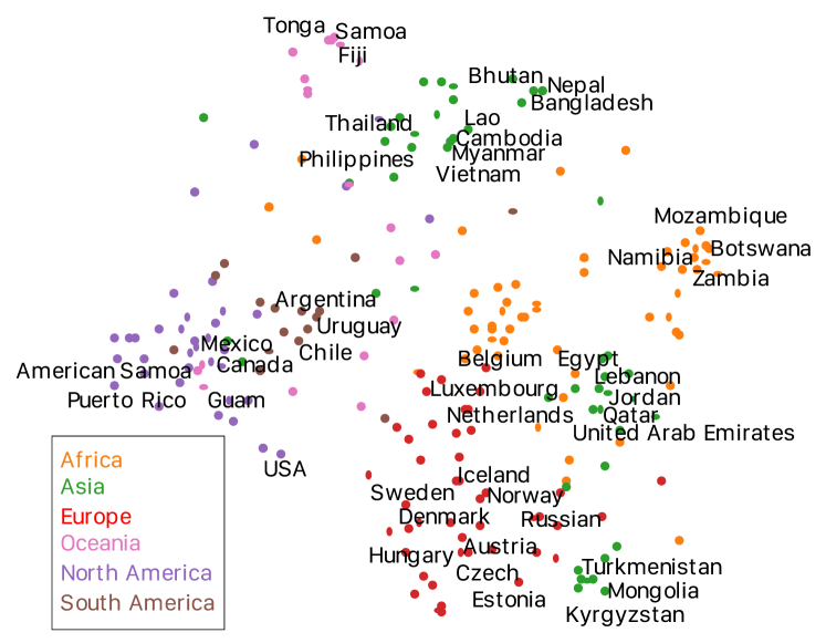
Figure 2. The interaction vectors capture the geographic and political relationship between countries.

Definition 0 (Entity Transaction Metric Sequence).

An entity transaction metric sequence is a time series, denoted as $\textbf{M}_{\text{E}}\in\mathbb{R}^{\tau_{m}}$ where $\tau_{m}$ is the length of the time series. We use $\textbf{M}_{\text{E}}[i:j]$ to denote the subsequence starting at the $i$-th timestamp and end at the $j$-th timestamp.

The entity time series $\mathbf{T}_{\text{E}}$ and entity transaction metric sequence $\textbf{M}_{\text{E}}$ have the identical length (i.e., $\tau_{e}=\tau_{m}$) since $\mathbf{T}_{\text{E}}$ and $\textbf{M}_{\text{E}}$ have the same sampling rate in our system. Specifically, $\textbf{M}_{\text{E}}$ stores each country’s target hourly transaction metric, and we have $\tau_{m}=8,760$ for a year with 365 days. Although the target metric in the implemented system is a uni-variate time series, it is possible to extend the proposed approach to multi-variate metric sequence with techniques introduced in (Yeh et al., 2020b). Based on above definitions, the problem that our system solves is:

Definition 0.

Given a time step $i$, an entity $E$, the entity interaction vector $\mathbf{I}_{\text{E}}[i]$, and the entity time series $\mathbf{T}_{\text{E}}[i-t_{p}:i]$, the goal of the transaction metric estimation problem is to learn a model $\mathsf{F}$ that can be used to predict the transaction metric of the entity between time $i-t_{a}$ and $i+t_{b}$, where $t_{a}$ and $t_{b}$ are the number of backward and forward time-steps to estimate, respectively. The model $\mathsf{F}$ can be formulated as follows: $\hat{\textbf{M}}_{\text{E}}[i-t_{a}:i+t_{b}]\leftarrow\mathsf{F}\left(\mathbf{T}_{\text{E}}[i-t_{p}:i],\mathbf{I}_{\text{E}}[i]\right)$ where $\hat{\textbf{M}}_{\text{E}}[i-t_{a}:i+t_{b}]$ is the estimated transaction metric from $i-t_{a}$ to $i+t_{b}$.

As suggested by the notation $\hat{\textbf{M}}_{\text{E}}[i-t_{a}:i+t_{b}]$, the estimated transaction metric is multi-horizontal (Yeh et al., 2020b; Zhuang et al., 2020). The decision to perform multi-horizon prediction is essential for our system because it creates buffer time between each consecutive prediction to ensure there is no downtime in the production environment. Specifically, our system predicts the target metric for the next 24 hours ($t_{b}=24$). Additionally, estimating the past for some transaction metrics is also necessary because there is a lengthy delay before the system can obtain the actual metrics. The estimation system can generate a more accurate estimation for analysis by observing the entities’ latest transaction behavior before the true target metric becomes available. Our system estimates the target transaction metric for the past 24 hours ($t_{a}=24$). For the input entity time series, we only look back $t_{p}$ time-step instead of using all the available time series for better efficiency. In our implementation, we look back 168 hours (i.e., $t_{p}=168$, seven days), and the past target metric is not part of the input to $\mathsf{F}$ because of the delay before the system could observe the actual target transaction metric is longer than seven days. Figure 3 shows how different time windows (i.e., $t_{p}$, $t_{a}$, and $t_{b}$) are located temporally relative to the current time step.

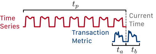
Figure 3. Relationship between the current time with various time windows (i.e., $t_{p}$, $t_{a}$, and $t_{b}$).

Given a training set consisting of both the entity time series and the entity interaction vectors from timestamp $1$ to $\tau_{e}$ for each $E\in\mathbb{E}$, model $\mathsf{F}$ is trained by minimizing the following loss function:

(1) $$\sum_{E\in\mathbb{E},i\in[1,\tau_{e}]}\texttt{loss}\left(\hat{\textbf{M}}_{\text{E}}\left[i-t_{a}:i+t_{b}\right],\textbf{M}_{\text{E}}\left[i-t_{a}:i+t_{b}\right]\right)$$

where $\texttt{loss}()$ can be any commonly seen regression loss function, e.g. mean squared error.

3. Model Architecture

Figure 4 depicts the overall architecture of our country-level transaction metric estimation model. The proposed model has five components: 1) interaction encoder, 2) temporal encoder, 3) scale decoder, 4) shape decoder, and 5) amalgamate layer. The two encoders extract hidden representations (i.e., $\mathbf{h}_{\text{I}}$ and $\mathbf{h}_{\text{T}}$) from the inputs (i.e., $\mathbf{I}_{\text{E}}$ and $\mathbf{T}_{\text{E}}$) independently. That is, each encoder is only responsible for one aspect of the input entity. Using the two extracted hidden representations, each decoder then independently provides information regarding different aspects of the estimated transaction metric sequence. The scale decoder provides the scale information (i.e., magnitude and offset), and the shape decoder provides the shape information. Lastly, the amalgamate layer combines the shape and scale information to generate the estimated transaction metric sequence.

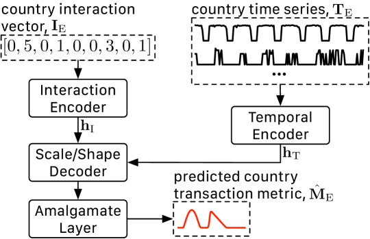
Figure 4. The transaction metric estimation model predicts the transaction metric for a period of time based on the input country’s interaction vector and time series.

[Interaction Encoder] is responsible for processing the entity interaction vectors $\mathbf{I}_{\text{E}}\in\mathbb{R}^{k}$ where $k$ is the number of entities in the model. The output interaction hidden representation $\mathbf{h}_{\text{I}}\in\mathbb{R}^{n_{k}}$ captures the information about the interactions between different entities in the database where $n_{k}$ is the embedding size for each entity. Following (Yeh et al., 2020c), we use a simple embedding-based model design shown in Figure 5.

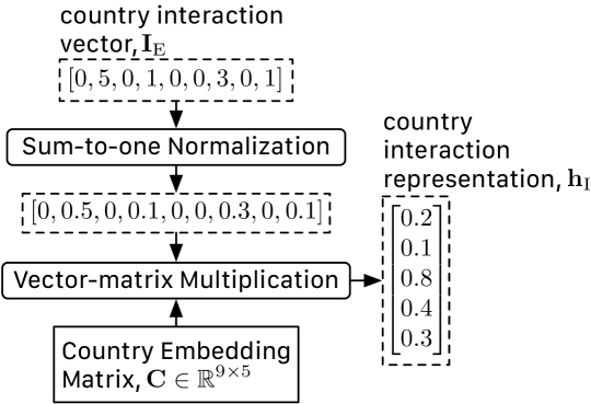
Figure 5. The design of the interaction encoder. Here, for demo purpose, we define the number of country as 9 and the embedding size as 5.

The input interaction vector is first normalized by the sum-to-one normalization. This step is important for modeling interaction between different entities in transaction database (Yeh et al., 2020c). Because the $L1$ vector norm of the input interaction vector is proportional to each country’s population, sum-to-one normalization ensures that the hidden representation focus on capturing the information regarding the interaction between different countries instead of the population difference.

With the normalized country interaction vector $\bar{\mathbf{I}}_{\text{E}}$, the interaction hidden representation $\mathbf{h}_{\text{I}}$ is computed with $\bar{\mathbf{I}}_{\text{E}}\textbf{C}$. The matrix C here contains the embeddings corresponding to each country. In other words, the interaction hidden representation $\mathbf{h}_{\text{I}}$ is a weighted sum of the embeddings in C. The matrix C is the only learnable parameter in the interaction encoder. It can either be initialized randomly or using existing embedding learned with the technique proposed in (Yeh et al., 2020a). The size of the returned interaction hidden representation $\mathbf{h}_{\text{I}}$ depends on each country’s embedding vector size. In our implementation, the number of countries is 233, and the size of the embedding vector is set to 64. Note, although we only model one type of interaction among the entities in our prototype, we can extend our system to handle multiple interaction types by using more interaction encoders.

[Temporal Encoder] extracts temporal hidden representation $\mathbf{h}_{\text{T}}$ $\in\mathbb{R}^{n_{k}}$ from the input entity time series $\mathbf{T}_{\text{E}}\in\mathbb{R}^{t_{p}\times d}$ where $n_{k}$ is the size of output hidden representation vector, $t_{p}$ is the length of the input time series, and $d$ is the dimensionality of the input time series. For the particular system presented in this paper, $n_{k}$ is 64, $t_{p}$ is 168, and $d$ is 14. As shown in Figure 6, the temporal encoder is designed based on the Temporal Convolutional Network (TCN) (Bai et al., 2018) with modification suggested by (Yeh et al., 2020c).

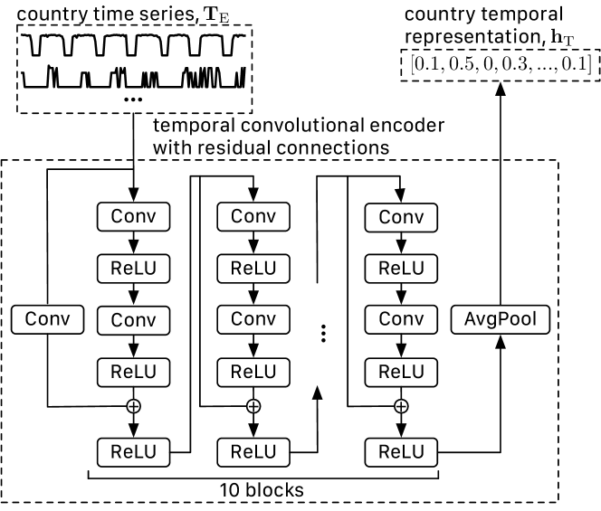
Figure 6. The design of the temporal encoder is a variant of temporal convolutional net with residual connection.

The body of the model consists of a sequence of identical residual blocks. The main passage is processed with Conv-ReLU-Conv-ReLU then combined with the output of residual passage before passing through a ReLU layer. The only exception is the first residual block where it has a Conv layer used to solve the shape mismatch problem between the output of the main passage and the residual passage. In our implementation, all the Conv layer has 64 kernels. The kernel size for all the Conv layers is 3 except the Conv layer in the first residual passage. The kernel size for the Conv layer in the first residual passage is 1 as its main purpose is to match the output shape of the main passage and the residual passage. The output temporal hidden representation is generated by summarizing the residual blocks’ output across time with the global average pooling (i.e., AvgPool) layer. Because the last Conv layer has 64 kernels, the output temporal hidden representation $\mathbf{h}_{\text{T}}$ is a vector of length 64.

[Scale Decoder] combines temporal hidden representation $\mathbf{h}_{\text{T}}$ and interaction hidden representation $\mathbf{h}_{\text{I}}$ to generate the scale (i.e., magnitude $\sigma$ and offset $\mu$) for the transaction metric sequence. The structure of the scale decoder is shown in Figure 7 which extends the structure proposed in (Yeh et al., 2020b) to also consider the interaction hidden representation $\mathbf{I}_{\text{E}}$ when predicting the scale.

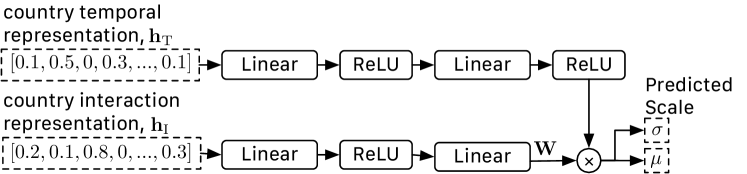
Figure 7. The scale decoder generates the magnitude $\sigma$ and offset $\mu$ based on the input hidden representations $\mathbf{h}_{\text{I}}$ and $\mathbf{h}_{\text{T}}$.

The Linear-ReLU-Linear-ReLU on the top further process the temporal hidden representation $\mathbf{h}_{\text{T}}$ to focus on the information relevant for predicting the scale. The Linear-ReLU-Linear on the bottom produce a matrix $\mathbf{W}\in\mathbb{R}^{n_{k}\times 2}$ which is used for mapping the output of the top Linear-ReLU-Linear-ReLU process to $\sigma$ and $\mu$. The motivation behind the design is that we assume entities with similar interaction representations should use similar $\mathbf{W}$ to estimate the scale of the target transaction metric sequence.

[Shape Decoder] is responsible for providing the shape estimation for the predicted transaction metric sequence. It combines temporal hidden representation $\mathbf{h}_{\text{T}}$ and interaction hidden representation $\mathbf{h}_{\text{I}}$ to generate the shape prediction. The structure of shape decoder is similar to the scale decoder as shown in Figure 8.

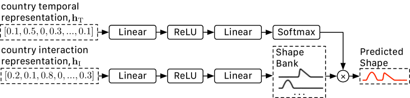
Figure 8. The shape decoder focuses on predicting the shape using the input hidden representations $\mathbf{h}_{\text{I}}$ and $\mathbf{h}_{\text{T}}$.

There are two differences between the design of shape decoder comparing to the design of scale encoder: 1) the output of the Linear-ReLU-Linear for processing interaction hidden representation $\mathbf{h}_{\text{I}}$ is a shape bank (Yeh et al., 2020b) which stores basis shapes for estimating the shape of the target transaction metric sequence and 2) the last layer for processing the temporal hidden representation $\mathbf{h}_{\text{T}}$ is a Softmax layer instead of a ReLU layer. The output of the Softmax layer dictates which and how the shape bank’s basic shapes are combined to form the shape prediction. Such a unique design is borrowed from (Yeh et al., 2020b), which has been shown to outperform alternative methods for transaction data. Similar to the scale decoder, we assume that entities with similar interaction representations should use similar basis shapes to estimate the shape of the target transaction metric sequence.

If we only consider the last two layers of the Linear-ReLU- Linear-Softmax passage for processing $\mathbf{h}_{\text{T}}$, this sub-model is a softmax regression model. Because the softmax regression model’s output is positive and always sum-to-one, it forces the model to pick only the relevant basis shapes for the prediction. As shown in the example presented in Figure 8, the predicted shape is generated by combining mostly the first two basis shapes in the shape bank. This design provides users a way to understand what the model learned from the data by looking at the shape bank’s content.

[Amalgamate Layer] combines the scale and shape information with $\hat{\mathbf{M}}_{\text{E}}^{\text{shape}}\times\sigma+\mu$ where $\hat{\mathbf{M}}_{\text{E}}^{\text{shape}}$ is the predicted shape, $\sigma$ contains the magnitude information, and $\mu$ contains the offset information. Following (Yeh et al., 2020b), we minimize the following loss function: $\sum_{E\in\mathbb{E}}\texttt{MSE}\left(\hat{\mathbf{M}}_{\text{E}},\mathbf{M}_{\text{E}}\right)+\gamma\texttt{NMSE}\left(\hat{\mathbf{M}}_{\text{E}}^{\text{shape}},\mathbf{M}_{\text{E}}\right)$ where $\texttt{MSE}()$ is a function computes the mean squared error, $\texttt{NMSE}()$ is a function computes the normalized mean squared error, $\gamma$ is a hyper-parameter to make sure the output of $\texttt{MSE}()$ and $\texttt{NMSE}()$ are in similar scale, and $\hat{\mathbf{M}}_{\text{E}}$ is the output of amalgamate layer,. $\texttt{NMSE}()$ is computed by first $z$-normalizing (Rakthanmanon et al., 2012) ground truth, then calculating the mean squared error between the $z$-normalized ground truth and $\hat{\mathbf{M}}_{\text{E}}^{\text{shape}}$.

4. Online Learning Scheme

We focus our investigation on refining Stochastic Gradient Descent-based optimization methods. This family of methods performs well for handling concept drift under online learning scenarios (Hoi et al., 2018; Losing et al., 2018) and is widely applied in the training of deep learning models (LeCun et al., 2012). Algorithm 1 shows the training scheme for our system. The input to the algorithm is a set of targeted entities that users wish to model, and the output is the estimated transaction metric sequence generated daily.

Algorithm 1 The Training Algorithm

1Input: set of target entities $\mathbb{E}$

2Output: estimated transaction metric sequence $\hat{\mathbf{M}}_{\text{E}}$

3function train($\mathbb{E}$)

4    $\mathsf{F}\leftarrow\texttt{InitializeModel}()$

5    $\mathsf{F}\leftarrow\texttt{OfflineTraining}(\mathsf{F},\mathbb{E})$

6    while True do

7        if time to update is False then

8           continue         

9        $\mathbb{E}\leftarrow\texttt{GetLatestAvailableData}()$

10        for $b\leftarrow 0$ to $n_{\mathrm{iter}}$ do

11           $\mathbf{I}_{\text{E},b},\mathbf{T}_{\text{E},b},\mathbf{M}_{\text{E},b}\leftarrow\texttt{ GetMiniBatch}(\mathbb{E})$

12           $\mathsf{F}\leftarrow\texttt{UpdateModel}\left(\mathbf{I}_{\text{E},b},\mathbf{T}_{\text{E},b},\mathbf{M}_{\text{E},b}\right)$         

13        $\hat{\mathbf{M}}_{\text{E}}\leftarrow\texttt{Estimation}(\mathsf{F},\mathbb{E})$

14        return $\hat{\mathbf{M}}_{\text{E}}$     

First, the estimation model is initialized in Line 2. Next, in Line 3, the initialized model is first trained offline with all the available data. The model goes into an online mode when entering the loop beginning at Line 4. In Line 5 and Line 6, the function checks if it is time to update the model. The model is updated daily. If it is time to update the model, the latest data is pulled from the transaction database in Line 7. From Line 8 to Line 10, the model is updated for $n_{\mathrm{iter}}$ iterations. Mini-batch for training are sampled in Line 9. We aim to refine this sampling step that is crucial for updating the model in an online learning setup as updating the model with “irrelevant” data could hurt the performance when concept drift is encountered.

In addition to the baseline uniform sampling method that is commonly seen in training deep learning model, we have tested a total of seven different special sampling techniques for sampling mini-batch when updating the model during online training. We group these seven different sampling techniques into two categories: temporal-based and non-temporal-based sampling methods. The temporal-based sampling method consists of methods that sample based on the temporal location of each candidate samples. The following three temporal-based sampling methods are tested.

• Fixed Window samples the training examples within the latest $x$ days uniformly where $x$ is a hyper-parameter for this method. In other words, it ignores older data.

• Time Decay samples the training examples with a decaying probability as the data aging. The probability decays linearly in our implementation.

• Segmentation (Gharghabi et al., 2017, 2019) (i.e., time series segmentation) can be used to identify a good window and time decay function in a data driven fashion. We have modified the method presented in (Gharghabi et al., 2017, 2019) for our problem. We present the modification in Section 4.1.

For non-temporal-based methods, the temporal location of each candidate sample is not considered in the sampling process. The following four non-temporal-based methods are explored.

• Similarity biases toward examples those are more similar to the current input time series $\mathbf{T}_{\text{E}}[i-t_{p}:i]$, where $i$ is the current time. As it only looks at the $\mathbf{T}_{\text{E}}$, it can only help the case where the concept drift affects $\mathbf{T}_{\text{E}}$. We use MASS algorithm (Mueen et al., 2017) to compute the similarity.

• High Error biases toward “hard” examples for the current model. Pushing the model to focus on hard examples is commonly seen in boosting-based ensemble methods (Schapire, 2003), and we are testing this idea for our problem.

• Low Error biases toward examples that can be predicted well based on the current model. Because the targeted transaction metric can be noisy sometimes, this sampling strategy could remove noisy samples since noisy samples tend to introduce large errors.

• Training Dynamic based sampling method has been proven effective for classification tasks (Swayamdipta et al., 2020). Particularly, it uses measures such as confidence and variability to sample data. We have computed the confidence and variability, mostly following the formulation presented in (Swayamdipta et al., 2020). Because (Swayamdipta et al., 2020) focuses on a different objective (i.e., classification), we modify the original probability distribution-based formulation to an error-based formulation for computing the confidence and variability. We test four sampling strategies using these two measures: 1) high confidence, 2) low confidence, 3) high variability, and 4) low variability.

With the updated model, estimating the transaction metric sequence using the latest data is generated in Line 11 and returned in Line 12. Note, as Algorithm 1 is an online learning algorithm the while loop continues after the model is output in Line 12.

4.1. Time Series Segmentation

Our time series segmentation-based sampling method is modified from the FLUSS algorithm (Gharghabi et al., 2017, 2019); it is built on top of the matrix profile idea (Yeh et al., 2016; Yeh et al., 2017; Yeh et al., 2018). The matrix profile is a way to efficiently explore the nearest neighbor relationship between subsequences of a time series (Zhu et al., 2016; Yeh, 2018). Because each candidate example for our model is a subsequence of the entity time series, we adopt a matrix profile-based method for our problem. We use Algorithm 2 to compute the sampling probability of each candidate for each entity in the training data. The input to the algorithm is the entity time series. We only use the part of the time series where the ground truth transaction metric is available.

Algorithm 2 The Modified FLUSS Algorithm

1Input: Entity time series $\mathbf{T}_{\text{E}}$

2Output: Sampling probability $P$

3function getProb($\mathbf{T}_{\text{E}}$)

4    for $j\leftarrow 1$ to $d$ do

5        $T_{j,\texttt{MPI}}\leftarrow\texttt{GetMatrixProfileIndex}(\mathbf{T}_{\text{E}}^{j})$

6        $T_{j,\texttt{CAC}}\leftarrow\texttt{GetCorrectedArcCount}(T_{j,\texttt{MPI}})$

7        $P\leftarrow\texttt{Add}(T_{j,\texttt{CAC}})$     

8    $p_{\texttt{min}}\leftarrow\texttt{inf}$

9    for $j\leftarrow\texttt{length}(P)$ to $1$ do

10        if $P[j]<p_{\texttt{min}}$ then

11           $p_{\texttt{min}}\leftarrow P[j]$

12        else

13           $P[j]\leftarrow p_{\texttt{min}}$             

14    $P\leftarrow\frac{P}{\texttt{Sum}(P)}$

15    return $P$

From Line 2 to Line 5, each iteration of the loop processes each dimension of the entity time series independently. In Line 3, the matrix profile index (Yeh et al., 2016) of the input time series’s $i$-th dimension is computed. The matrix profile index shows the nearest neighbor of each subsequence in the input time series with subsequence length $t_{p}$. As shown in Figure 9a, we can connect each subsequence with its nearest neighbor using an arc based on the information stored in the matrix profile index.

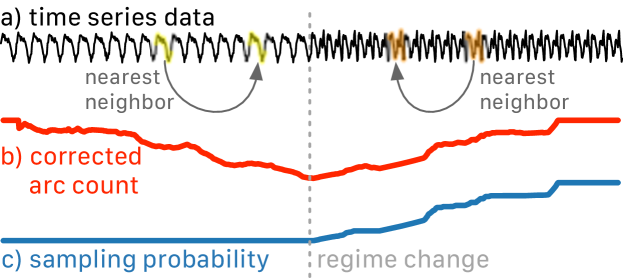
Figure 9. The sampling probability is computed from the corrected arc count curve.

To further process the matrix profile index, we compute the corrected arc count (CAC) curve (Gharghabi et al., 2017). The curve records the number of arcs passing through each temporal location. We use a correction method proposed in (Gharghabi et al., 2017) to correct the fact that it is more likely to have an arc passing through the center relative to the two ends of the time series. The correction method corrects the count by comparing the actual count to the expected count. As the first half and second half of the time series data shown in Figure 9a are different, and the arc only connects similar subsequences, there is almost no arc passing through the center of the time series, and the CAC curve is low in the center (see Figure 9b). To combine the CAC curve of each dimension, similar to (Gharghabi et al., 2019), we just add the CAC curve together in Line 5.

Once the CAC curve is computed, we need to convert the CAC curve to sampling probability. In Lines 6 -- 11, we use the loop to enforce the non-decreasing constrain. The goal is to ensure the subsequences belonging to the newest regime (i.e., subsequences after the latest segmentation point) have higher sampling probability than those from the old regime. As demonstrated in Figure 9c, the non-decreasing constraint flattens the CAC curve before the regime change. Lastly, the non-decreasing CAC curve is converted to a probability curve in Line 12 and returned in Line 13.

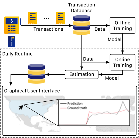
Figure 10. System design of the proposed system. The system consists of an offline training stage prior to deployment, a daily routine when the system is deployed, and a graphical user interface for users to monitor the system.

5. System Implementation

As presented in Section 4, the proposed transaction metric estimation system has two training phases: the offline and the online training phases. Before deployment, the offline training module retrieves the latest data from the transaction database to train the initial model. Once we deploy the initial model, the online training module and estimation module would be activated daily at midnight. The online training module first updates the current model using the best online learning scheme established in Section 6.2 with available data from the transaction database. Next, the estimation module produces the target transaction metric estimation for the succeeding 24 hours and the preceding 24 hours. We then stored the predictions in a database. The user can monitor the system with a graphical user interface (GUI) by either visually evaluating the most recent prediction or comparing the previous prediction with ground truth data if the ground truth data is available. Figure 10 depicts the overall design of the system.

In the implemented prototype system, we store raw transaction data in the Hadoop Distributed File System (HDFS) (The Apache Software Foundation, 2021a). Because of the sheer volume of transaction data, we perform most of the data processing jobs in Hadoop and generate hourly aggregated multivariate time series using Apache Hive (The Apache Software Foundation, 2021b). We then move these hourly-aggregated time series to a local GPU sever for offline and online training with PyTorch (Paszke et al., 2019). The inference/prediction is also performed on the GPU server, and the corresponding results are maintained/updated in a MySQL (Oracle Corporation and/or its affiliates, 2021) database. A web-based GUI is designed to facilitate the accessing from any client-side browsers. An example interface of our system is shown in Figure 10, which shows that users can flexibly fetch data for any country of interest from the map visualization.

6. Experiment

The models and optimization process are implemented with PyTorch 1.4 (Paszke et al., 2019) with Adam optimizer (Kingma and Ba, 2014). The similarity search (i.e., MASS (Mueen et al., 2017)) and matrix profile (Yeh et al., 2016) computation are handled by Matrix Profile API (Van Benschoten et al., 2020). We use country-wise aggregated transaction data from 1/1/2017 to 12/31/2017 as the training data, and data from 1/1/2018 to 12/31/2018 as the test data. To measure the performance, we use root mean squared error (RMSE), normalized root mean squared error (NRMSE) (Yeh et al., 2020b; Zhuang et al., 2020), and coefficient of determination ($R^{2}$).

6.1. Verification of the Model Architecture

In this section, we evaluate different design decisions regarding our model architecture. Notably, we test the benefit of using both entity interaction vectors and entity time series, the advantage of using the shape/scale decoder design, and comparing our best model configuration with alternative methods. We use two different temporal encoder designs for this section: 1) the convolutional neural network (CNN) which uses the design presented in Figure 6 and 2) two layers of gated recurrent units (GRUs) (Cho et al., 2014). We only test GRU instead of long short-term memory (LSTM) because it has been established in (Yeh et al., 2020c, b; Zhuang et al., 2020) that GRU has similar or superb performance comparing to LSTM when processing time series generated from transaction data. In each subsequent subsection, we add a new mechanism to the base models and observe the before-and-after performance difference.

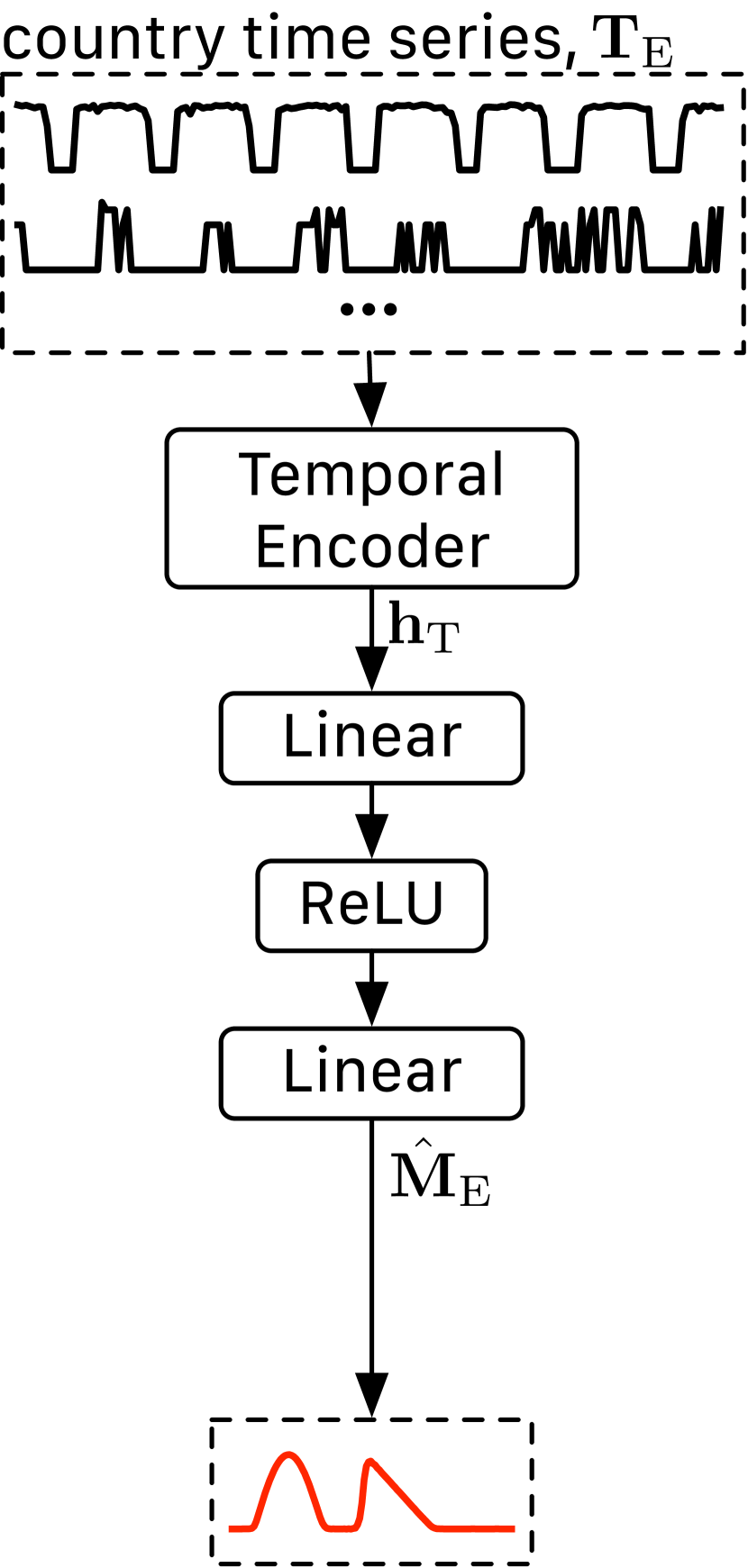
(a) base model

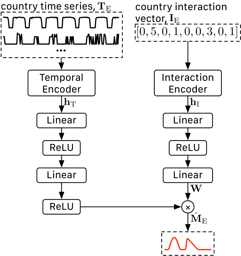
(b) base model + interaction vector

Figure 11. The proposed model design is compared with these baseline model designs.

6.1.1. Benefit of Interaction Vector

First, we examine the benefit of modeling both entity time series and entity interaction vector. The base model (i.e., Figure 11(a)) we consider only uses entity time series because it consists of richer information regarding each entity in transaction data comparing to the interaction vector as demonstrated in (Yeh et al., 2020c). To evaluate the benefit of modeling both entity time series and interaction vector, we compare the base model to a more straightforward multimodality design proposed in (Yeh et al., 2020c) (i.e., Figure 11(b)). The model shown in Figure 11(b) is simpler comparing to the model presented in Figure 4 as it does not use shape/scale-decoder design. Because neither the base model nor the multimodality model estimate the shape and scale separately, they are trained by minimizing the MSE loss function instead. The passage processing the interaction hidden representation $\mathbf{I}_{\text{E}}$ outputs a matrix $\mathbf{W}\in\mathbb{R}^{n_{k}\times(t_{a}+t_{b})}$ which is multiplied by the output of the passage process the time series hidden representation $\mathbf{h}_{\text{T}}$ to generate the prediction $\hat{\mathbf{M}}_{\text{E}}$. Table 1 shows the improvement of using multimodality model comparing to the base model for both CNN-based and GRU-based temporal encoder design. Note, the base models are the baseline deep learning models.

Table 1. Using both time series and interaction vector improves the performance.

	CNN-based Encoder			GRU-based Encoder
	RMSE	NRMSE	$R^{2}$	RMSE	NRMSE	$R^{2}$
Base	8.2741	0.8545	0.1493	7.7352	0.8287	0.1943
Base + Inter.	7.3165	0.8256	0.2026	7.0617	0.8098	0.2268
% Improved	11.6%	3.4%	35.7%	8.7%	2.3%	16.7%

The improvement is consistent across the three different performance measurements for both temporal encoder designs. The percent improvement is considerably more for $R^{2}$ comparing to other performance measurements. The percent improvement for the models with CNN-based temporal encoder is more prominent than the models with GRU-based temporal encoder. Overall, GRU-based temporal encoder performs slight better than the CNN-based temporal encoder.

Table 2. Shape/scale decoder design improves the performance.

	CNN-based Encoder			GRU-based Encoder
	RMSE	NRMSE	$R^{2}$	RMSE	NRMSE	$R^{2}$
Base + Inter.	7.3165	0.8256	0.2026	7.0617	0.8098	0.2268
Proposed	5.7147	0.7386	0.2771	6.4736	0.7426	0.2598
% Improved	21.9%	10.5%	36.8%	8.3%	8.3%	14.6%

6.1.2. Benefit of Shape/Scale Decoder Design

Next, we would like to confirm whether the shape/scale decoder design (i.e., Figure 4) can further improve the performance. We compare it to the base model shown in Figure 11(b), which was the superior model design based on the experiment presented in Section 6.1.1. Table 2 shows how the shape/scale decoder design (i.e., the proposed design) further improves the performance.

Once again, the improvement is consistent across the three performance measurements for both temporal encoder designs. The percent improvement is more noticeable for $R^{2}$ comparing to other performance measurements. The percent improvement for the models with CNN-based temporal encoder is remarkably more than the models with GRU-based temporal encoder. The best model configuration according to both Table 1 and Table 2 is the proposed design with CNN-based temporal encoder (i.e., Figure 4).

6.1.3. Comparison with Alternative Methods

The last thing we want to confirm with our model design is how does it compare to commonly seen off-the-shelf machine learning solutions in production environments. Particularly, we compare our best configuration with ready-to-deploy models like a linear model, $k$ nearest neighbor, random forest, and gradient boosting. The result is shown in Table 3. The hyper-parameters for the alternative methods are determined using 5-fold cross-validation with training data. The percent improvement is computed against the best alternative based on each performance measurement.

Table 3. The proposed method outperforms common off-the-shelf machine learning models in production environment.

Method	RMSE	NRMSE	$R^{2}$
Linear Model	9.1732	1.1039	0.0312
$k$ Nearest Neighbor	6.2690	0.8452	0.2217
Random Forest	6.0354	0.8224	0.2172
Gradient Boosting	7.7524	0.8670	0.1638
Proposed	5.7147	0.7386	0.2771
% Improved	4.4%	10.2%	27.3%

Out of the four rival methods, the two more competitive ones are the $k$ nearest neighbor ($k$NN) and random forest (RF), where the $k$NN has the best $R^{2}$ while RF has the best RMSE and NRMSE. When comparing the proposed model’s $R^{2}$ with $k$NN’s $R^{2}$, we see a $27.3\%$ improvement. When comparing the proposed model’s RMSE and NRMSE with RF’s RMSE and NRMSE, we see a $4.4\%$ and $10.2\%$ improvement, respectively. The proposed model outperforms the rivals more in NRMSE and $R^{2}$ based on the percent improvement. As both NRMSE and $R^{2}$ are computed in a “normalized” scale and measure how the estimated trend matches the ground truth, the proposed model captures more details in the transaction metric sequence than alternative methods. Note, the base models presented in Table 1 are the baseline deep learning-based models.

6.2. Evaluation of Online Learning Schemes

To further improve the system’s performance, we use the online learning framework presented in Section 4 to update the model as the system receiving previously unavailable training data. Each day, the system receives the ground truth of the date 90 days before the current day. The system then uses the newly received data and the existing training data to update the model. The number of iteration $n_{\mathrm{iter}}$ used in Algorithm 1 is 100, and the batch size is 1,024.

6.2.1. Is Online Learning Necessary?

Before we compare different online learning methods, we first confirm whether performing online learning to deployed model is the right decision. We compare the offline learning model with the naive online learning model where the model is updated with Algorithm 1 using baseline sampling method (i.e., uniform sampling). The experiment result is summarized in Table 4.

Table 4. Baseline online learning model outperforms the offline learning model.

Method	RMSE	NRMSE	$R^{2}$
Offline	5.7147	0.7386	0.2771
Online Baseline	5.5240	0.7159	0.3258
% Improved	3.3%	3.1%	17.6%

Online learning technique does improve the performance noticeably, especially the $R^{2}$. To provide further motivation for refining the online learning method before showcasing the benchmark experiment, we present the performance gain of our best performing online learning method (i.e., segmentation + similarity) comparing to the baseline online learning method in Table 5. The best performing online learning method identified by our benchmark experiment is capable of further enhancing the system.

Table 5. Using the best online learning model the performance can be further improved.

Method	RMSE	NRMSE	$R^{2}$
Online Baseline	5.5240	0.7159	0.3258
Online Best	5.3800	0.7000	0.3400
% Improved	2.6%	2.2%	4.4%

6.2.2. What is the Best Online Learning Scheme?

To determine the best online learning scheme out of all the schemes outlined in Section 4 for our system, we have performed a benchmark experiment with our dataset. For the fixed window method, we test it with a window size of 90 days (i.e., one season) and 365 days (i.e., one year). In addition to testing the listed methods alone, we also test every combination between a temporal-based and non-temporal-based methods. To combine the probabilities from two methods, we multiply the sampling probability of one method with the other method’s sampling probability. We test a total of 40 different online learning schemes on six different model architectures from Section 6.1. For each model, we compute each online learning scheme’s rank based on either the RMSE, NRMSE, or $R^{2}$; then, for each online learning scheme, we compute the average rank across the six different model architectures.

The result is presented in Table 6 and Table 7. Because the presented number is average rank, the tables’ values are the lower, the better. We also compute the mean of average rank for each row and column to help interpret the results. Each cell is color based on its average rank relative to the baseline (i.e., Uniform+Uniform). If the result in a cell is better than the baseline, the cell is colored with blue. If the result in a cell is worse than the baseline, the cell is colored with orange.

Table 6. Averaged ranking of each online learning scheme based on RMSE.

RMSE	Uniform	Fix (90)	Fix (365)	Decay	Segment	Average
Uniform	21.00	22.44	15.67	18.33	16.11	18.71
Similar	16.22	19.56	14.11	12.00	17.00	15.78
High-error	28.00	32.44	29.00	28.00	30.22	29.53
Low-error	12.11	9.89	8.44	9.22	7.22	9.38
High-confidence	14.67	17.11	12.78	11.67	11.67	13.58
Low-confidence	33.44	37.44	32.44	32.22	34.00	33.91
High-variability	25.44	31.11	26.00	23.56	27.11	26.64
Low-variability	20.33	19.89	14.89	14.11	13.11	16.47
Average	21.40	23.74	19.17	18.64	19.56

Table 6 presented the RMSE-based average rank of different online learning schemes. When considering different temporal-based methods, Fix (365), Decay, and Segment constantly outperform the Uniform baseline. Generally, to learn a better model with lower RMSE, the model needs to see data more than 90 days old as 90 days fixed window performs worse than the baseline. For non-temporal-based methods, Similar, Low-error, High-confidence, and Low-variability outperform the baseline. Because Low-error, High-confidence, and Low-variability push the model to focus on “easy” or “consistent” examples in the training data, the improvement is likely caused by the removal of noisy training examples for our data set. Overall, combining Low-Error with Segment gives the best result when the performance is measured with RMSE.

Table 7. Averaged ranking of each online learning scheme based on NRMSE.

NRMSE	Uniform	Fix (90)	Fix (365)	Decay	Segment	Average
Uniform	29.11	11.78	20.00	30.00	7.11	19.60
Similar	16.22	7.22	9.67	7.33	2.56	8.60
High-error	35.11	24.67	30.00	25.56	17.67	26.60
Low-error	28.00	9.78	18.89	15.67	6.56	15.78
High-confidence	28.33	13.33	21.78	15.44	6.33	17.04
Low-confidence	37.22	34.67	34.00	28.22	23.22	31.47
High-variability	32.78	27.22	28.00	25.22	19.22	26.49
Low-variability	29.67	13.11	22.89	17.56	8.89	18.42
Average	29.56	17.72	23.15	20.63	11.45

According to NRMSE-based average rank (Table 7), for temporal-based methods, Segment gives superior performance comparing to others. When combining Segment with different non-temporal-based methods, the conclusion is similar to Table 6, the better methods are Similar, Low-error, High-confidence, and Low-variability. Overall, combining Similar with Segment gives the best result when the performance is measured with NRMSE. It is almost always the best method for each tested model architecture. We also compute average rank with $R^{2}$, because the conclusion is similar to Table 7 we omit the table for brevity.

In conclusion, both Similar+Segment and Low-Error+Segment is a good choice as both have great average ranks in all performance measurements. On one hand, Similar+Segment has top performances when consider both NRMSE and $R^{2}$; therefore, we should pick Similar+Segment if NRMSE and $R^{2}$ are more important. On the other hand, although Low-Error+Segment does not have outstanding NRMSE and $R^{2}$, it has the best RMSE-based average rank. Low-Error+Segment should be used when RMSE is more critical for the application. Since we care more about capturing the trend rather than the raw values for our system, we choose to deliver the model trained with Similar+Segment as prototype. The delivered model’s performance is shown in the second row of Table 5.

7. Related Work

We focus our review on research works studying online learning and time series perdition problems. The reasons are: 1) the proposed transaction metric estimation system utilizes online learning techniques, and 2) time series perdition models inspire the proposed model architecture design.

Online learning is a supervised learning scenario where the training data are made available incrementally in a streaming fashion. A common challenge when developing a system under such a scenario is handling a phenomenon called concept drift (Schlimmer and Granger, 1986; Gama et al., 2014). Over the years, several survey/benchmark papers of various scopes have been written on this topic (Žliobaitė, 2010; Gama et al., 2014; Krawczyk et al., 2017; Hoi et al., 2018; Losing et al., 2018; Lu et al., 2018). There are many facets to the development of an online learning solution for the concept drift problem. For example, detection of concept drift is a popular sub-problem studied in (Bifet and Gavalda, 2007; Liu et al., 2017; Yu and Abraham, 2017). There are also online learning solutions focusing on adapting a specific machine learning model to the concept drift like (Platt, 1998) for support vector machine, (Oza, 2005) for boosting algorithm, and (Losing et al., 2016) for $k$ nearest-neighbor model. Developing application-specific solutions like (Jia et al., 2017), which is designed for land cover prediction, is another common research direction. This work focuses on developing an online learning method specific for a deep learning-based transaction metric estimation system.

Time series prediction or forecasting is a research area with many different problem settings (De Gooijer and Hyndman, 2006; Box et al., 2015; Faloutsos et al., 2019). The proposed transaction metric estimation system is mainly focused on a variant of the problem called multi-horizon time series prediction (Taieb and Atiya, 2015). There have been many models proposed for the multi-horizon time series prediction problem (Taieb and Atiya, 2015; Wen et al., 2017; Shih et al., 2019; Fan et al., 2019; Zhuang et al., 2020; Yeh et al., 2020b). Taieb and Atiya (Taieb and Atiya, 2015) test multiple multi-horizon time series prediction strategies and show making multi-horizon prediction by merely making a 1-step recursive prediction is not always the best strategy. Wen et al. (Wen et al., 2017) combine the direct strategy from (Taieb and Atiya, 2015) with various recurrent neural network-based model architecture for multi-horizon time series prediction. Zhuang et al. (Zhuang et al., 2020) further refine the recurrent neural network-based model to capture the hierarchical temporal structure within the input time series data. Aside from recurrent neural network-based model, Fan et al. (Fan et al., 2019) examine the possibility of adopting an attention mechanism for multi-horizon time series prediction. Shih et al. (Shih et al., 2019) propose a network structure that combines ideas from the attention mechanism and convolution neural network. Sen et al. (Sen et al., 2019) combine convolutional neural network-based design and matrix factorization model to capture the time series’s local and global properties at the same time. Based on similar principles, (Yeh et al., 2020b) propose a convolutional neural network-based network design with sub-networks dedicated to capturing the “shape” and “scale” information of time series data independently. The model used in the proposed transaction metric estimation system is inspired by works introduced in this paragraph with an extension to handle the multimodal nature of our transaction data.

8. Conclusion and Future Work

We propose an online transaction metric estimation system that consists of a user-facing interface, an online adaptation module, and an offline training module. We present a novel model design and demonstrate its superb performance compared with the alternatives. Further, we show the benefit of applying online learning schemes to the problem. To identify the best online learning scheme for our system, we perform a detailed set of experiments comparing existing and novel online learning schemes. The proposed system not only been used as a monitoring tool, but also provides the predicted metrics as features to our in-house fraud detection system. For future work, we are looking into applying the findings to other entities from payment network like merchants, issuers, or acquirers. We are also interested in exploring the possibility of test the system on data from other domains.

References

- (1)
- Bai et al. (2018) Shaojie Bai, J Zico Kolter, and Vladlen Koltun. 2018. An empirical evaluation of generic convolutional and recurrent networks for sequence modeling. arXiv preprint arXiv:1803.01271 (2018).
- Bifet and Gavalda (2007) Albert Bifet and Ricard Gavalda. 2007. Learning from time-changing data with adaptive windowing. In Proceedings of the 2007 SIAM international conference on data mining. SIAM, 443–448.
- Box et al. (2015) George EP Box, Gwilym M Jenkins, Gregory C Reinsel, and Greta M Ljung. 2015. Time series analysis: forecasting and control. John Wiley & Sons.
- Cho et al. (2014) Kyunghyun Cho, Bart Van Merriënboer, Caglar Gulcehre, Dzmitry Bahdanau, Fethi Bougares, Holger Schwenk, and Yoshua Bengio. 2014. Learning phrase representations using RNN encoder-decoder for statistical machine translation. arXiv preprint arXiv:1406.1078 (2014).
- De Gooijer and Hyndman (2006) Jan G De Gooijer and Rob J Hyndman. 2006. 25 years of time series forecasting. International journal of forecasting 22, 3 (2006), 443–473.
- Faloutsos et al. (2019) Christos Faloutsos, Valentin Flunkert, Jan Gasthaus, Tim Januschowski, and Yuyang Wang. 2019. Forecasting Big Time Series: Theory and Practice. In Proceedings of the 25th ACM SIGKDD International Conference on Knowledge Discovery & Data Mining. ACM, 3209–3210.
- Fan et al. (2019) Chenyou Fan, Yuze Zhang, Yi Pan, Xiaoyue Li, Chi Zhang, Rong Yuan, Di Wu, Wensheng Wang, Jian Pei, and Heng Huang. 2019. Multi-horizon time series forecasting with temporal attention learning. In Proceedings of the 25th ACM SIGKDD International Conference on Knowledge Discovery & Data Mining. 2527–2535.
- Gama et al. (2014) João Gama, Indrė Žliobaitė, Albert Bifet, Mykola Pechenizkiy, and Abdelhamid Bouchachia. 2014. A survey on concept drift adaptation. ACM computing surveys (CSUR) 46, 4 (2014), 1–37.
- Gharghabi et al. (2017) Gharghabi et al. 2017. Matrix profile VIII: domain agnostic online semantic segmentation at superhuman performance levels. In 2017 IEEE International Conference on Data Mining (ICDM). IEEE, 117–126.
- Gharghabi et al. (2019) Gharghabi et al. 2019. Domain agnostic online semantic segmentation for multi-dimensional time series. Data mining and knowledge discovery 33, 1 (2019), 96–130.
- Hoi et al. (2018) Steven CH Hoi, Doyen Sahoo, Jing Lu, and Peilin Zhao. 2018. Online learning: A comprehensive survey. arXiv preprint arXiv:1802.02871 (2018).
- Jia et al. (2017) Xiaowei Jia, Ankush Khandelwal, Guruprasad Nayak, James Gerber, Kimberly Carlson, Paul West, and Vipin Kumar. 2017. Incremental dual-memory lstm in land cover prediction. In Proceedings of the 23rd ACM SIGKDD International Conference on Knowledge Discovery and Data Mining. 867–876.
- Kapur et al. (2020) Girish Kapur, Bharat Prasad, and Nathan Nickels. 2020. Solving Merchant Attrition using Machine Learning. https://medium.com/@ODSC/solving-merchant-attrition-using-machine-learning-989e41e81b0e.
- Kingma and Ba (2014) Diederik P Kingma and Jimmy Ba. 2014. Adam: A method for stochastic optimization. arXiv preprint arXiv:1412.6980 (2014).
- Krawczyk et al. (2017) Bartosz Krawczyk, Leandro L Minku, João Gama, Jerzy Stefanowski, and Michał Woźniak. 2017. Ensemble learning for data stream analysis: A survey. Information Fusion 37 (2017), 132–156.
- LeCun et al. (2012) Yann A LeCun, Léon Bottou, Genevieve B Orr, and Klaus-Robert Müller. 2012. Efficient backprop. In Neural networks: Tricks of the trade. Springer, 9–48.
- Liu et al. (2017) Anjin Liu, Yiliao Song, Guangquan Zhang, and Jie Lu. 2017. Regional concept drift detection and density synchronized drift adaptation. In IJCAI International Joint Conference on Artificial Intelligence.
- Losing et al. (2016) Viktor Losing, Barbara Hammer, and Heiko Wersing. 2016. KNN classifier with self adjusting memory for heterogeneous concept drift. In 2016 IEEE 16th international conference on data mining (ICDM). IEEE, 291–300.
- Losing et al. (2018) Viktor Losing, Barbara Hammer, and Heiko Wersing. 2018. Incremental on-line learning: A review and comparison of state of the art algorithms. Neurocomputing 275 (2018), 1261–1274.
- Lu et al. (2018) Jie Lu, Anjin Liu, Fan Dong, Feng Gu, Joao Gama, and Guangquan Zhang. 2018. Learning under concept drift: A review. IEEE Transactions on Knowledge and Data Engineering 31, 12 (2018), 2346–2363.
- Maaten and Hinton (2008) Laurens van der Maaten and Geoffrey Hinton. 2008. Visualizing data using t-SNE. Journal of machine learning research 9, Nov (2008), 2579–2605.
- Mora (2019) Andreu Mora. 2019. Predicting and monitoring payment volumes with Spark and ElasticSearch. https://www.adyen.com/blog/predicting-and-monitoring-payment-volumes-with-spark-and-elasticsearch.
- Mueen et al. (2017) Abdullah Mueen, Yan Zhu, Chin-Chia Michael Yeh, Kaveh Kamgar, Krishnamurthy Viswanathan, Chetan Gupta, and Eamonn Keogh. 2017. The fastest similarity search algorithm for time series subsequences under euclidean distance.
- Oracle Corporation and/or its affiliates (2021) Oracle Corporation and/or its affiliates. 2021. MySQL™. https://www.mysql.com/.
- Oza (2005) Nikunj C Oza. 2005. Online bagging and boosting. In 2005 IEEE international conference on systems, man and cybernetics, Vol. 3. Ieee, 2340–2345.
- Paszke et al. (2019) Adam Paszke, Sam Gross, Francisco Massa, Adam Lerer, James Bradbury, Gregory Chanan, Trevor Killeen, Zeming Lin, Natalia Gimelshein, Luca Antiga, et al. 2019. Pytorch: An imperative style, high-performance deep learning library. In Advances in neural information processing systems. 8026–8037.
- Pearson ([n.d.]) Jamie Pearson. [n.d.]. Real-time Payments Analytics - Prediction. https://www.ir.com/blog/payments/real-time-payments-analytics-prediction.
- Platt (1998) John Platt. 1998. Sequential minimal optimization: A fast algorithm for training support vector machines. (1998).
- Rakthanmanon et al. (2012) Thanawin Rakthanmanon, Bilson Campana, Abdullah Mueen, Gustavo Batista, Brandon Westover, Qiang Zhu, Jesin Zakaria, and Eamonn Keogh. 2012. Searching and mining trillions of time series subsequences under dynamic time warping. In Proceedings of the 18th ACM SIGKDD international conference on Knowledge discovery and data mining. 262–270.
- Schapire (2003) Robert E Schapire. 2003. The boosting approach to machine learning: An overview. In Nonlinear estimation and classification. Springer, 149–171.
- Schlimmer and Granger (1986) Jeffrey C Schlimmer and Richard H Granger. 1986. Incremental learning from noisy data. Machine learning 1, 3 (1986), 317–354.
- Sen et al. (2019) Rajat Sen, Hsiang-Fu Yu, and Inderjit S Dhillon. 2019. Think globally, act locally: A deep neural network approach to high-dimensional time series forecasting. In Advances in Neural Information Processing Systems. 4838–4847.
- Shih et al. (2019) Shun-Yao Shih, Fan-Keng Sun, and Hung-Yi Lee. 2019. Temporal pattern attention for multivariate time series forecasting. Machine Learning 108, 8-9 (2019), 1421–1441.
- Swayamdipta et al. (2020) Swabha Swayamdipta, Roy Schwartz, Nicholas Lourie, Yizhong Wang, Hannaneh Hajishirzi, Noah A Smith, and Yejin Choi. 2020. Dataset Cartography: Mapping and Diagnosing Datasets with Training Dynamics. arXiv preprint arXiv:2009.10795 (2020).
- Taieb and Atiya (2015) Souhaib Ben Taieb and Amir F Atiya. 2015. A bias and variance analysis for multistep-ahead time series forecasting. IEEE transactions on neural networks and learning systems 27, 1 (2015), 62–76.
- The Apache Software Foundation (2021a) The Apache Software Foundation. 2021a. Apache Hadoop™. https://hadoop.apache.org/.
- The Apache Software Foundation (2021b) The Apache Software Foundation. 2021b. Apache Hive™. https://hive.apache.org/.
- Thomas (2020) Arun Thomas. 2020. Atm cash-out: The biggest threat we ignore. https://medium.com/@netsentries/atm-cash-out-the-biggest-threat-we-ignore-d0d4f3e50096.
- Van Benschoten et al. (2020) Andrew H Van Benschoten, Austin Ouyang, Francisco Bischoff, and Tyler W Marrs. 2020. MPA: a novel cross-language API for time series analysis. Journal of Open Source Software 5, 49 (2020), 2179.
- Wen et al. (2017) Ruofeng Wen, Kari Torkkola, Balakrishnan Narayanaswamy, and Dhruv Madeka. 2017. A multi-horizon quantile recurrent forecaster. arXiv preprint arXiv:1711.11053 (2017).
- Yeh (2018) Chin-Chia Michael Yeh. 2018. Towards a Near Universal Time Series Data Mining Tool: Introducing the Matrix Profile. arXiv preprint arXiv:1811.03064 (2018).
- Yeh et al. (2020a) Chin-Chia Michael Yeh, Dhruv Gelda, Zhongfang Zhuang, Yan Zheng, Liang Gou, and Wei Zhang. 2020a. Towards a Flexible Embedding Learning Framework. arXiv preprint arXiv:2009.10989 (2020).
- Yeh et al. (2017) Chin-Chia Michael Yeh, Nickolas Kavantzas, and Eamonn Keogh. 2017. Matrix profile vi: meaningful multidimensional motif discovery. In 2017 IEEE international conference on data mining (ICDM). IEEE, 565–574.
- Yeh et al. (2016) Chin-Chia Michael Yeh, Yan Zhu, Liudmila Ulanova, Nurjahan Begum, Yifei Ding, Hoang Anh Dau, Diego Furtado Silva, Abdullah Mueen, and Eamonn Keogh. 2016. Matrix profile I: all pairs similarity joins for time series: a unifying view that includes motifs, discords and shapelets. In 2016 IEEE 16th international conference on data mining (ICDM). Ieee, 1317–1322.
- Yeh et al. (2018) Chin-Chia Michael Yeh, Yan Zhu, Liudmila Ulanova, Nurjahan Begum, Yifei Ding, Hoang Anh Dau, Zachary Zimmerman, Diego Furtado Silva, Abdullah Mueen, and Eamonn Keogh. 2018. Time series joins, motifs, discords and shapelets: a unifying view that exploits the matrix profile. Data Mining and Knowledge Discovery 32, 1 (2018), 83–123.
- Yeh et al. (2020b) Chin-Chia Michael Yeh, Zhongfang Zhuang, Wei Zhang, and Liang Wang. 2020b. Multi-future Merchant Transaction Prediction. arXiv preprint arXiv:2007.05303 (2020).
- Yeh et al. (2020c) Chin-Chia Michael Yeh, Zhongfang Zhuang, Yan Zheng, Liang Wang, Junpeng Wang, and Wei Zhang. 2020c. Merchant Category Identification Using Credit Card Transactions. arXiv preprint arXiv:2011.02602 (2020).
- Yu and Abraham (2017) Shujian Yu and Zubin Abraham. 2017. Concept drift detection with hierarchical hypothesis testing. In Proceedings of the 2017 SIAM International Conference on Data Mining. SIAM, 768–776.
- Zhang et al. (2020) Wei Zhang, Liang Wang, Robert Christensen, Yan Zheng, Liang Gou, and Hao Yang. 2020. Transaction sequence processing with embedded real-time decision feedback. US Patent App. 16/370,426.
- Zhu et al. (2016) Zhu et al. 2016. Matrix profile ii: Exploiting a novel algorithm and gpus to break the one hundred million barrier for time series motifs and joins. In 2016 IEEE 16th international conference on data mining (ICDM). IEEE, 739–748.
- Zhuang et al. (2020) Zhongfang Zhuang, Chin-Chia Michael Yeh, Liang Wang, Wei Zhang, and Junpeng Wang. 2020. Multi-stream RNN for Merchant Transaction Prediction. arXiv preprint arXiv:2008.01670 (2020).
- Žliobaitė (2010) Indrė Žliobaitė. 2010. Learning under concept drift: an overview. arXiv preprint arXiv:1010.4784 (2010).