Black holes as frozen stars

Abstract

We have recently proposed a model for a regular black hole, or an ultra-compact object, that is premised on having maximally negative radial pressure throughout the entirety of the object’s interior. This model can be viewed as that of a highly entropic configuration of fundamental, closed strings near the Hagedorn temperature, but from the perspective of an observer who is ignorant about the role of quantum physics in counteracting against gravitational collapse. The advantage of this classical perspective is that one can use Einstein’s equations to define a classical geometry and investigate its stability. Here, we complete the model by studying an important aspect of this framework that has so far been overlooked: The geometry and composition of the outermost layer of the ultra-compact object, which interpolates between the bulk geometry of the object and the standard Schwarzschild vacuum solution in its exterior region. By imposing a well-defined set of matching conditions, we find a metric that describes this transitional layer and show that it satisfies all the basic requirements; including the stability of the object when subjected to small perturbations about the background solution. In fact, we are able to show that, at linearized order, all geometrical and matter fluctuations are perfectly frozen in the transitional layer, just as they are known to be in the bulk of the object’s interior.

1 Introduction

The final state of matter collapsing under its own gravity, what is now universally known as a black hole (BH), had been initially termed as a “frozen star” [1]. From the perspective of an outside observer, the collapse continues, formally, for an infinite period of time and deviations from the static Schwarzschild geometry decay exponentially in time. The scale for the latter is the light-crossing time across the collapsing star, and having such a short time scale for perturbations to decay means that the star is essentially “frozen”.

The rebranding of frozen stars as BHs came about once the singular nature of their classical solutions was finally confirmed. The first efforts along this line can be traced to the likes of Raychaudhuri [2] and Komar [3]. A further sign that something was amiss can be seen in the works of Buchdahl [4], Chandrasekhar [5, 6] and Bondi [7], who used the formalism of general relativity to show that “normal” matter cannot be stable when confined to a small-enough radius. Penrose and Hawking formalized these ideas in mathematical terms with their singularity theorems [8, 9].

As singularities are untenable in the quantum realm because of the associated violations of unitarity, a common assumption is that regularity will be preserved once quantum mechanics is correctly incorporated. A popular expectation is that quantum effects at the Planck scale will resolve the BH singularity and replace infinities with large-but-finite densities. However, attempts at realizing this expectation have so far failed to succeed. As it turns out, if the resolution scale is much smaller than the Schwarzschild scale, then the quantum emission of particles from the object will be such that the emitted energy greatly exceeds the original BH mass [10, 11]. Our conclusion, therefore, is that deviations from general relativity that extend over horizon-sized scales should be a minimal requirement for a non-singular BH.

Ultra-compact objects (UCOs) have become shorthand for extremely dense astrophysical objects that are regular but otherwise behave — for the most part — like the BHs of general relativity along with its standard semiclassical extensions. (See [12] for an exhaustive review and “status report”.) The collapsed polymer model of a BH [13] was born out of the idea that a viable UCO would be one that contains a maximally entropic fluid throughout its interior, which in turn means that it is described by a highly quantum state of exotic matter [14]. With inspiration from various sources [15, 16, 17, 18, 19], what was eventually proposed was a trans-Hagedorn configuration of long, closed and interacting strings. One finds that this polymer model can explain all known properties of Schwarzschild BHs [20]. Given a significant enough departure away from equilibrium [21], this description can also lead to novel predictions that may soon be testable using the observational data of gravitational waves [22, 23, 24, 25].

One notable drawback of using the polymer model to describe “real-world” astrophysical BHs is that its strongly non-classical state implies that the interior is lacking a semiclassical description [26, 27, 28]. Moreover, the Einstein equations have no room for entropy, which is rather awkward when it comes to describing a gravitating matter system whose defining feature is its highly entropic status. Thus the polymer model cannot be used to deal directly with questions of a geometric nature.

In [29] (also see [30]), we proposed a strategy for a classical description that captures important aspects of the polymer model, but as it would be viewed by someone who is ignorant about the importance of quantum mechanics in describing gravitational collapse. To elaborate on the strategy, let us first recall that the polymer model has the largest possible pressure $p$ that is allowed by causality $\;p=\rho\;$ ($\rho$ is the energy density), as this condition translates into the desired feature of maximal entropy $\;s=\frac{1}{T}(\rho+p)\;$ ($s$ is the entropy density and $T$ is the temperature). But an observer who knows nothing about the quantum nature of the interior will set the entropy density $s$ to zero. And so what once was a maximally positive pressure has now become maximally negative, $\;p=-\rho\;$, when viewed from this classical perspective. Indeed, maximally negative pressure is just what is needed to evade the singularity theorems [8, 9], as well as the Buchdahl bound [4] and similar limits [5, 6, 7]. See [31] for further discussion on this point.

The frozen star shares some similarities with other UCOs that exploit large negative pressure such as the black star [32], the gravastar [33] and even a (sort of) hybrid of the two [34]. More specifically, the frozen star can be viewed as a limiting case of the black star, whereas the main distinction between the gravastar and our model has to do with the (an)isotropy of the pressure. Unlike the isotropic nature of the gravastar pressure, our model has a maximally negative radial component $p_{r}$, whereas the other (transverse) components $p_{\perp}$ are regarded as vanishing, at least on average. Having a preferential spatial coordinate is quite natural given the spherical symmetry of the frozen star.

The geometry of the frozen star, although regular, is quite unusual (however, see [35, 36]). It has the especially peculiar feature that $\;g_{tt}=g^{rr}=0\;$ at all points within the interior. This can again be traced to its association with the polymer model for which maximal entropy means that the Bekenstein–Hawking entropy bound [37, 38] is saturated at every radius less than or equal to the Schwarzschild radius. In other words, every spherical shell from the center up to the outer surface behaves just like a horizon.

The combination of $\;g_{tt}=g^{rr}=0\;$ and $\;p_{r}+\rho=0\;$ is rather restrictive; in fact, these conspire to prescribe a background solution that fails to support any form of small fluctuations of the metric and the matter densities, justifying the term frozen star. This was evident from an inspection of the linearized Einstein equations, as elaborated on in [29].

With a hat tip to nostalgia, we will now refer to this classicalized version of the polymer BH as a “frozen star”.

An important but previously unaddressed question is what exactly does happen at the outermost layer of the collapsed polymer/frozen star model. This would be difficult to answer from the polymer perspective, but the expectation is that the energy density and pressure decrease in a continuous way over a string-scale distance from their interior values to zero, as does the entropy density. Translated to the classical frozen star model, the geometry can be expected to interpolate smoothly between the exotic interior and the Schwarzschild exterior. This is, however, far from being trivial as the smoothing has to happen over a small-enough length scale to ensure the persistence of the model’s main features. But even if such a solution does exist, there is the additional question of whether or not perturbative stability is maintained when this type of transitional layer is incorporated [39]. There are also some concerns about the extremely large transverse pressures that are part and parcel with this type of setup [40].  Our current objective is to address these issues by using the classically geometric framework of the frozen star model.

The presentation proceeds as follows: First, we confirm the existence of a suitable metric for the transitional layer near the outer boundary. This metric is obtained by matching an appropriate ansatz to both the bulk interior and the Schwarzschild exterior at appropriate interfaces, while insisting on the continuity of various geometric quantities and matter fields. Many of the details of this procedure and some supporting analysis are deferred to an appendix. Next, the important issue of stability is addressed. We conclude with a discussion on why large transverse pressures in the transitional layer are no cause for concern, followed by a brief overview of our results.

Conventions

We assume a spherically symmetric and static background spacetime with $\;D=3+1\;$ spacetime dimensions, although a similar analysis and conclusions will persist for any $\;D>3\;$. All fundamental constants besides Newton’s constant $G$ are set to unity throughout. In the stability analysis, we further fix $\;8\pi G=1\;$. A prime (dot) indicates a radial (temporal) derivative.

2 A metric for the transitional layer

2.1 The bulk

Before discussing the crust — the thin transitional layer between the bulk and the boundary — we first recall some basics about the interior bulk of the frozen star. Let us begin with a static and spherically symmetric line element,

$$ds^{2}\;=\;-f(r)dt^{2}+\frac{1}{{\widetilde{f}}(r)}dr^{2}+r^{2}(d\theta^{2}+sin^{2}\theta d\phi^{2})\;.$$ (1)

It is then assumed (as discussed above) that the radial pressure is maximally negative, $\;p_{r}=-\rho\;$. The transverse components $p_{\perp}$ are, on the other hand, left unspecified for the time being. All of the off-diagonal elements of the stress tensor are vanishing.

Under these conditions, Einstein’s equations reduce to

$$\left(r{\widetilde{f}}\right)^{\prime} \;=\;1-8\pi G\rho r^{2}\;,$$ (2)

$$\left(rf\right)^{\prime\prime}\; \;=\;16\pi Grp_{\perp}\;.$$ (3)

Given that $\;f={\widetilde{f}}\;$, the previous pair are equivalent to

$$\left(\rho r^{2}\right)^{\prime}\;=\;-2rp_{\perp}\;,$$ (4)

which is then consistent with the conservation of the stress tensor.

Let us next define

$$m(r)\;=\;4\pi\int\limits_{0}^{r}dx\,x^{2}\rho(x)\;\;\;{\rm for}\;\;\;r\leq R\;.$$ (5)

One then finds that

$$f(r)\;=\;{\widetilde{f}}(r)\;=\;1-\frac{2m(r)}{r}\;.$$ (6)

The functional form of $\rho(r)$ or, equivalently, $m(r)$, is what ultimately determines the geometry of the UCO. For instance, the gravastar solution is determined by the choice $\rho={\rm const}.$; in other words, a de Sitter interior. As the frozen star should be the classical analogue of the polymer model — for which the entropy–area law is saturated throughout — the natural choice is to saturate the Schwarzschild limit $\;m(r)=r/2\;$, also throughout. Equivalently, $\;\rho\sim 1/r^{2}$. We thus end up with the advertised outcome of $\;f=0\;$ and the matter densities can be shown to adopt the following profiles:

$$8\pi G\rho = \frac{1-(rf)^{\prime}}{r^{2}}\;=\;\frac{1}{r^{2}}\;,$$ (7)

$$8\pi Gp_{r} = -\frac{1-(rf)^{\prime}}{r^{2}}\;=\;-\frac{1}{r^{2}}\;,$$ (8)

$$8\pi Gp_{\perp} = \frac{(rf)^{\prime\prime}}{2r}\;=\;0\;.$$ (9)

2.2 The crust

We now want to implement the concept of a transitional layer in concrete terms. The UCO is regarded as having a radius of $R$, $\;r=R\;$ being the midpoint of a thin transitional layer. This layer will be taken to range from $\;r=r_{A}=R-\lambda\;$ to $\;r=r_{B}=R+\lambda\;$, where $\;\lambda\ll R\;$. Because of the star’s connection to the polymer model, we expect that $\lambda$ is of order of the string length $l_{s}$, $\;\lambda\sim l_{s}\;$, but its exact value is not important to the current work. What is important is that $\lambda$ is parametrically larger than the Planck length, so that the Einstein equations remain valid in the crust.

We start with the assumption that the key symmetries of the frozen star interior, $\;{\widetilde{f}}=f\;$ and $\;p_{r}=-\rho\;$, persist into the transitional layer. The form of the metric is found by adopting the ansatz that $f(r)$ is a polynomial expansion in terms of $\;\frac{r-r_{A}}{R}<\frac{2\lambda}{R}\;$. The order of the polynomial and, thus, the number of adjustable parameters in the ansatz is determined by the number of relevant boundary conditions. For this analysis, we are imposing that $f(r)$, $f^{\prime}(r)$ and $f^{\prime\prime}(r)$ be continuous at both ends of the layer. This means the imposition of the matching conditions $\;f=f^{\prime}=f^{\prime\prime}=0\;$ at $\;r=r_{A}\;$, as well as matching $f$ and its first two derivatives to their standard Schwarzschild values at $\;r=r_{B}\;$. This procedure results in a fifth-order polynomial, as described in the Appendix. Additional conditions could be imposed, if one so desires, but at the cost of additional parameters. We were satisfied with these six because they were enough to ensure the continuity of all the stress-tensor components, as well as their first derivatives, at both ends of the layer. In Fig. 1, we depict the metric function and the stress-tensor components in the transitional layer for various values of $\lambda$.

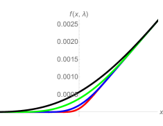
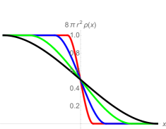
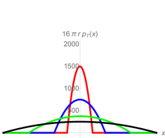
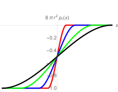
Figure 1: The panel depicts, for several values of the dimensionless width parameter $\lambda/R$, the metric function $f$ (upper left), the energy density (upper right), the transverse pressure (lower left) and the radial pressure (lower right) as a function of the dimensionless parameter $x=r/R$. The vertical axis is positioned at $x=1$ in the middle of the transitional layer, $x<1$ corresponds to the part of the transitional layer closer to the bulk and $x>1$ to the part closer to the exterior.

In spite of the simplicity of the methodology, the actual expressions are quite complicated and so have been relegated to the Appendix along with some supporting analysis. What is worth emphasizing is that $f$ and $\rho$ are non-negative throughout the spacetime (cf, Sections A.6 and A.7). The same can be said about $p_{\perp}$ (see A.8), ensuring that the null energy condition is never violated. It is also worth a mention that, in the layer itself, $\;\frac{1}{r}(r^{2}\rho)^{\prime}\sim-\frac{R}{\lambda}\rho\;$, meaning that $\;p_{\perp}\sim\frac{R}{\lambda}\rho\gg\rho\;$; cf, Eq. (4).  A large transverse pressure is an inevitable consequence of trying to increase a maximally negative $p_{r}$ to zero over a small length scale, as first elaborated on within [40] in reference to the gravastar model. Why this is not really a bad thing for our model will be the focus of the fourth section.

3 Linear ultra-stability

It was shown in [29] that, for the frozen star, all linear fluctuations about the background solution are vanishing; the star is not just stable but “ultra-stable”. This outcome was not unexpected because of an analysis in [20] (following a similar one in [17]) which revealed that perturbations of the polymer’s equilibrium state die out exponentially quickly. But, in the case of the frozen star, the stability can best be attributed to a pair of strong constraints on the background solution; namely, $\;p_{r}+\rho=0\;$ and $\;f=-g_{tt}=g^{rr}=0\;$. However, the status of the latter changes in the transitional layer as the metric function $f(r)$ is no longer vanishing. Still, it will be shown that the ultra-stability persists by virtue of the continuity of the metric through the interface at $r=r_{A}$. To this end, we will be following Chandrasekhar’s linear stability analysis [5, 6].

For the rest of this section, the zeroth-order matter functions carry a subscript of 0 and $\;8\pi G=1\;$.

The metric and stress tensor are now expressible as

$$g_{\mu\nu} \;=\; \text{diag}\Biggl{(}-f(r)+\delta g_{tt}(t,r),\ \ 1/f(r)+\delta g_{rr}(t,r),\ \ r^{2},\ \ r^{2}\sin^{2}\theta\Biggr{)}\;$$ (10)

$$\;=\; \text{diag}\Biggl{(}-f(r)(1-H_{0}(t,r)),\ \ 1/f(r)(1+H_{2}(t,r)),\ \ r^{2},\ \ r^{2}\sin^{2}\theta\Biggr{)}\;\ \ \ \ \$$ (11)

and

$$T^{\mu}_{\;\;\nu}\;=\;\text{diag}\Biggl{(}-{\rho}_{0}-\delta\rho,\ \ -{\rho}_{0}+\delta p_{r},\ \ {p}_{\perp}{}_{0}+\delta p_{\perp},\ \ {p}_{\perp}{}_{0}+\delta p_{\perp}\Biggr{)}\;.$$ (12)

Let us next consider, one by one, the perturbed forms of the (non-trivial) Einstein equations, as well as the perturbed conservation equation. We are assumed to be working strictly in the transitional layer as defined in the previous section, $\;R-\lambda\leq r\leq R+\lambda\;$ or $\;r_{A}\leq r\leq r_{B}\;$.

The ${}^{t}_{\ r}$ equation is

$$\dot{H}_{2}(t,r)\;=\;\tfrac{r}{f(r)}\left(\rho_{0}+p_{r}{}_{0}\right)\text{v}_{r}\;,$$ (13)

where $\;\text{v}_{r}=\dot{r}\;$ is the radial velocity and we use this to further define the Lagrangian displacement $\xi$ such that $\;\text{v}_{r}=\partial_{t}\xi\;$. Integrating this equation with respect to time, one then obtains

$$H_{2}(t,r)\;=\;\tfrac{r}{f(r)}\left(\rho_{0}+p_{r}{}_{0}\right)\xi\;.$$ (14)

But, since $\;\rho_{0}+p_{r}{}_{0}=0\;$, it immediately follows that

$$H_{2}(t,r)\;=\;0\;.$$ (15)

This is consistent with the bulk analysis [29] and continuity. The conclusion is that $g_{rr}$ is frozen at its background value throughout the transitional crust, just as it is for the bulk interior.

The ${}^{t}_{\ t}$ equation takes the form

$$-\frac{1}{r^{2}}+\frac{f+rf^{\prime}}{r^{2}}-\frac{f+rf^{\prime}}{r^{2}}H_{2}(t,r)-\frac{f}{r^{2}}H^{\prime}_{2}\;=\;-\rho_{0}-\delta\rho(t,r)\;.$$ (16)

Identifying $\rho_{0}$ from Eq. (7) and using the vanishing of $H_{2}$, we find that $\delta\rho$ is also frozen,

$$\delta\rho(t,r)\;=\;0\;.$$ (17)

The ${}^{r}_{\ r}$ equation goes as

$$-\frac{1}{r^{2}}+\frac{f+rf^{\prime}}{r^{2}}-\frac{f+rf^{\prime}}{r^{2}}H_{2}(t,r)-\frac{f}{r}H_{0}^{\prime}\;=\;p_{r}{}_{0}+\delta p_{r}(t,r)\;.$$ (18)

Identifying $p_{r}{}_{0}$ via Eq. (8) and taking $H_{2}$ to zero, we have

$$-\frac{f}{r}H_{0}^{\prime}\;=\;\delta p_{r}\;.$$ (19)

Meanwhile, the ${}^{\theta}_{\ \theta}$ equation leads to

$$-\frac{1}{2f}\partial_{t}^{2}H_{2} + \frac{2f^{\prime}+rf^{\prime\prime}}{2r}-\frac{2f^{\prime}+rf^{\prime\prime}}{2r}H_{2}(t,r)-\frac{f^{\prime}}{4}(3H_{0}^{\prime}+H_{2}^{\prime})$$ (20)

$$- \frac{1}{2r}(H_{0}^{\prime}+H_{2}^{\prime}+rH_{0}^{\prime\prime})\;=\;p_{\perp}{}_{0}+\delta p_{\perp}(t,r)\;.$$ (21)

With the identifications of $p_{\perp}{}_{0}$ from Eq. (9) and $\;H_{2}=0\;$,

$$-\frac{f}{2r}H_{0}^{\prime}-\tfrac{3}{4}f^{\prime}H_{0}^{\prime}-\frac{f}{2}H_{0}^{\prime\prime}\;=\;\delta p_{\perp}(t,r).$$ (22)

As for the conservation equation, once $\;H_{2}=0\;$, $\;\delta\rho=0\;$ and the zeroth-order terms are all accounted for, this becomes

$$\nabla_{\mu}T^{\mu}_{\ r}\;=\;-\frac{2}{r}(\delta p_{r}-\delta p_{\perp})+\tfrac{1}{2}\frac{f^{\prime}}{f}\delta p_{r}+\delta p_{r}^{\prime}=0\;.$$ (23)

Equation (23) can be turned, using Eqs. (19) and (22), into a differential equation for $H_{0}$ alone,

$$2\frac{f}{r^{2}}H_{0}^{\prime}-3\frac{f^{\prime}}{r}H_{0}^{\prime}-2\frac{f}{r}H_{0}^{\prime\prime}\;=\;0\;.$$ (24)

The most general solution for Eq. (24) is readily obtained,

$$H_{0}^{\prime}(t,r)\;=\;A(t)e^{\ \int\limits_{r_{A}}^{r}\left(\frac{3}{2}\frac{f^{\prime}}{f}-\frac{1}{r}\right)dr}+B(t)\;,$$ (25)

where $A(t)$ and $B(t)$ are integration “constants” which can be fixed at the inner boundary of the transitional region, $\;r=r_{A}\;$.

Recall from the prior section that the boundary conditions at $r_{A}$ are $\;f=f^{\prime}=f^{\prime\prime}=0\;$. Technically, these conditions apply only to the background geometry. But on this we can say more because $r_{A}$ is also part of the bulk interior where the fluctuations are all vanishing. So that, by continuity, $\;H_{0}=H_{0}^{\prime}=H_{0}^{\prime\prime}=0\;$ are also true at the $\;r=r_{A}\;$ interface. Let us first impose $\;H_{0}^{\prime}(r_{A})=0\;$ to obtain $\;B=-A\;$ and then $\;H_{0}^{\prime\prime}(r_{A})=0\;$ which leads to $\;A=0\;$, meaning that $\;H_{0}^{\prime}=0\;$ for all $r$. The result is that $H_{0}$ must be equal to a constant and, by further imposing $\;H_{0}(r_{A})=0\;$, we know that the constant in question is zero. This leads to the conclusion that $H_{0}$, just like $H_{2}$, is frozen throughout,

$$H_{0}\;=\;0\;.$$ (26)

Finally, Eqs. (19) and (22) now tell us that both types of pressure perturbations are vanishing, just like $\delta\rho$ was shown to be.

To summarize, we have found that all metric and matter perturbations vanish identically even when the frozen star has been topped off with an outer layer for which $\;f(r)\neq 0\;$.

4 Causality

As first discussed in [40] and noted above, any UCO model that is premised on the idea of a radial pressure that is large and negative will inevitably lead to very large transverse pressures in the boundary layer. An easy way to see this is to reconsider the stress-tensor conservation equation but with our previous condition of $\;\rho+p_{r}=0\;$ now being relaxed,

$$p^{\prime}_{r}+\frac{f^{\prime}}{f}(\rho+p_{r})+\frac{2}{r}(p_{r}-p_{\perp})=\;0\;\;.$$ (27)

For a negative radial pressure whose magnitude is the same order as the energy density, the middle term on the left-hand-side of Eq. (27) is parametrically smaller than the other two terms. Meanwhile, this large negative radial pressure has to increase to zero at the outer edge of a relatively thin transitional layer, thus making its radial derivative large. The transverse pressure is then left to compensate for this large value of $p^{\prime}_{r}$. The good news is that the transverse pressure must be positive to do its job, so that the null energy condition is never violated. There is, however, the issue of causality, as well as the physical interpretation of large transverse pressures for a static configuration with no external forces.

Let us start with the apparent violation of causality because of $\;p_{\perp}\sim\frac{R}{\lambda}\rho\gg\rho\;$ in the transitional layer. Fortunately, there are two ways — one local and one non-local — to see that $p_{\perp}\gg\rho$ does not translate, as one might perhaps expect, into sound speeds in excess of the speed of light. And so, in spite of appearances. the crust does not support superluminal propagation.

The local way is to calculate the transverse speed of sound $c_{S}{}_{\perp}$ via the thermodynamic relation $\;c^{2}_{S}{}_{\perp}=\left|\frac{\delta p_{\perp}}{\delta\rho}\right|\;$. This can be accomplished by applying the Euler—Lagrange equation directly to Eq. (27), along with the frozen star equation of state, $\;p_{r}=-\rho\;$,

$$-\partial_{r}\frac{\delta p_{r}}{\delta\rho}+\frac{f^{\prime}}{f}(1+\frac{\delta p_{r}}{\delta\rho})+\frac{2}{r}\left(\frac{\delta p_{r}}{\delta\rho}-\frac{\delta p_{\perp}}{\delta\rho}\right)\;=\;0\;.$$ (28)

The variation $\;\frac{\delta p_{r}}{\delta\rho}=-1\;$ leads to $\;c^{2}_{S}{}_{\perp}=1\;$, which is what a hypothetical local observer would measure for the speed of transverse-moving modes.

The non-local way of calculating the transverse speed of sound is to use the line element for the transitional layer, $\;c^{2}_{S}{}_{\perp}=r^{2}\frac{d\theta^{2}}{dt^{2}}=f(r)\;$. In this layer, a typical value of $f(r)$ is small but nonvanishing, $\;f(r)\sim\frac{\lambda}{R}\;$, which follows from $f(r)$ varying from 0 up to $\lambda/(R+\lambda)$ as per Eqs. (37) and (38) in the Appendix. This result for the transverse speed is what a distant observer would measure. However, to compare with the previous result, one must take the effect of the gravitational redshift into account, which essentially means dividing the transverse speed of sound $c_{S}{}_{\perp}$ by $\sqrt{f(r)}$, leading to $\;c^{2}_{S}{}_{\perp}=1\;$. Hence, the two calculations are in complete agreement, and we can conclude that there is no threat to causality.

It is tempting to suggest that the large transverse pressures are merely a mathematical artifact of maintaining energy conservation while inside the transitional layer. To support this claim, we can turn to the polymer perspective, where a maximally negative value of $p_{r}$ is, itself, a fictitious consequence of ignoring the maximally entropic state of the internal matter. Indeed, from this stringy point of view, one can set $\;p_{\perp}\approx 0\;$ throughout the transitional layer and can replace $p_{r}+\rho$ with $sT$ (again, approximately). The conservation equation (27) now looks like

$$p^{\prime}_{r}+\frac{f^{\prime}}{f}(sT)+\frac{2}{r}p_{r}\;=\;0\;.$$ (29)

In the polymer model, it is a maximally positive $p_{r}$ that must decline rapidly to zero in moving outwards through the transitional layer, so that $p^{\prime}_{r}$ is negative and of order $\rho/\lambda$. But this is exactly the same order as the (manifestly positive) entropic term. There is no need for a transverse pressure, large or otherwise, when viewed from this perspective.

Overview

We have shown that our frozen star model — which can be regarded as the geometrical manifestation of the polymer model for the BH interior — can readily incorporate a thin transitional layer at the outer surface of a so-described UCO. Notably, this outer crust maintains the same ultra-stability of the interior bulk and, furthermore, poses no threat to causality or the null energy condition.

These results could further our understanding on just how the collapsed polymer/frozen star model modifies the experimental signatures of gravitational waves emitted during a binary BH merger and of out-of-equilibrium physics from those of the general relativistic paradigm. See [21, 22, 23, 24, 25] for progress along these lines from a somewhat different perspective.

Appendix A The transitional layer in detail

The purpose of this Appendix is to give a detailed account of how we found the metric for the transitional layer. Also included is analysis in support of various statements that are made in the main text of the paper.

A.1 The model

We start here by recalling that our model — the frozen star — describes a 4-dimensional, static, spherically symmetric UCO of radius $R$, for which the radial component of the pressure is maximally negative, $\;p_{r}=-\rho\;$. Let us also revisit the line element (1), but now with the knowledge that $\;-g_{tt}=g^{rr}\;$ is required for consistency with the conservation of the stress tensor,

$$ds^{2}\;=\;-f(r)dt^{2}+\frac{1}{f(r)}dr^{2}+r^{2}(\sin^{2}\theta+d\phi^{2})\;.$$ (30)

Also recalled, from Section 2, are the expressions for the energy density, radial pressure and transverse pressure,

$$\rho(r)\;=\;\frac{1-f-rf^{\prime}}{8\pi Gr^{2}}\;,$$ (31)

$$p_{r}(r)\;=\;-\frac{1-f-rf^{\prime}}{8\pi Gr^{2}}\;,$$ (32)

$$p_{\perp}(r)\;=\;\frac{2f^{\prime}+rf^{\prime\prime}}{16\pi Gr}\;.$$ (33)

Finally, let us reiterate our proposed framework: The sphere is assumed to have an outermost transitional layer of thickness $\;2\lambda\ll R\;$, centered around $\;r=R\;$. That is, the layer is half inside and half outside of the sphere, as is conventional in problems involving the transition between two media. The inner boundary of the layer at $\;r=R-\lambda\;$ connects to the bulk interior (for which $f$ and all its derivatives vanish throughout) and its outer boundary at $\;r=R+\lambda\;$ connects to the Schwarzschild exterior. Effectively invoking Occam’s razor, we assume that the interior conditions $\;p_{r}+\rho=0\;$ and $\;g_{tt}+g^{rr}=0\;$ persist into the layer.

A.2 Continuity conditions for $f(r),\;f^{\prime}(r),\;f^{\prime\prime}(r)$

Let us begin here by matching $f$ and its first two derivatives at each of the two endpoints of the transitional layer. It can be checked that the continuity of these three functions is sufficient to ensure the continuity of the matter densities as well. To this end, we now introduce a function $S(r,\lambda)$ (with the $\lambda$ sometimes implied) that will be used to express $f$ in the layer,

$$f\;=\;\begin{cases}0,\quad r<R-\lambda\\ S(r),\quad R-\lambda<r<R+\lambda\\ 1-\frac{R}{r},\quad r>R+\lambda\;,\end{cases}$$ (34)

$$f^{\prime}\;=\;\begin{cases}0,\quad r<R-\lambda\\ S^{\prime}(r),\quad R-\lambda<r<R+\lambda\\ \frac{R}{r^{2}},\quad r>R+\lambda\;,\end{cases}$$ (35)

$$f^{\prime\prime}\;=\;\begin{cases}0,\quad r<R-\lambda\\ S^{\prime\prime}(r),\quad R-\lambda<r<R+\lambda\\ -\frac{2R}{r^{3}},\quad r>R+\lambda\;.\end{cases}$$ (36)

The matching conditions on $S(r,\lambda)$ at the layer’s endpoints are then as follows:

For the continuity of $f$,

$$1.\quad S(r=R-\lambda,\lambda)\;=\;0\;,$$ (37)

$$2.\quad S(r=R+\lambda,\lambda)\;=\;\frac{\lambda}{R+\lambda}\;.$$ (38)

For the continuity of $f^{\prime}$,

$$3.\quad S^{\prime}(r=R-\lambda,\lambda)\;=\;0\;,$$ (39)

$$4.\quad S^{\prime}(r=R+\lambda,\lambda)\;=\;\frac{R}{(R+\lambda)^{2}}\;.$$ (40)

And, for the continuity of $f^{\prime\prime}$,

$$5.\quad S^{\prime\prime}(r=R-\lambda,\lambda)\;=\;0\;,$$ (41)

$$6.\quad S^{\prime\prime}(r=R+\lambda,\lambda)\;=\;-\frac{2R}{(R+\lambda)^{3}}\;.$$ (42)

It is convenient at this point to introduce a dimensionless radial coordinate, $\;x=\frac{r}{R}\;$, so that the transitional layer $\;R-\lambda<r<R+\lambda\;$ can be alternatively defined as $\;1-\lambda<x<1+\lambda\;$.  In what follows, a prime indicates a radial derivative with respect to its argument and a derivative with respect to $r$ when no argument is provided.

A.3 Continuity conditions for $\rho(r),\;p_{r}(r),\;p_{\perp}(r)$

The energy density, radial pressure, and transverse pressure are re-expressed below in terms of the function $S(r,\lambda)$. One can readily verify our claim that the continuity of $\rho(r),\;p_{r}(r),\;{\rm and}\;p_{\perp}(r)$ through the endpoints of the translational layer is consistent with the conditions (37)-(42).

$$\rho\;=\;\begin{cases}\frac{1}{8\pi Gr^{2}},\quad r<R-\lambda\\ \frac{1-S(r)-rS^{\prime}(r)}{8\pi Gr^{2}},\quad R-\lambda<r<R+\lambda\\ 0,\quad r>R+\lambda\;,\end{cases}$$ (43)

$$p_{r}\;=\;\begin{cases}-\frac{1}{8\pi Gr^{2}},\quad r<R-\lambda\\ -\frac{1-S(r)-rS^{\prime}(r)}{8\pi Gr^{2}},\quad R-\lambda<r<R+\lambda\\ 0,\quad r>R+\lambda\;,\end{cases}$$ (44)

$$p_{\perp}\;=\;\begin{cases}0,\quad r<R-\lambda\\ \frac{2S^{\prime}(r)+rS^{\prime\prime}(r)}{16\pi Gr},\quad R-\lambda<r<R+\lambda\\ 0,\quad r>R+\lambda\;.\end{cases}$$ (45)

A.4 Continuity conditions for $\rho^{\prime}(r),\;p^{\prime}_{\perp}(r)$

The expressions for the first derivatives of the energy density and the transverse pressure take on the respective forms, 

$$\rho^{\prime}(r,\lambda)\;=\;\begin{cases}-\frac{2}{8\pi Gr^{3}},\quad r<R-\lambda\\ -\frac{2-2S(r)+r^{2}S^{\prime\prime}(r)}{8\pi Gr^{3}},\quad R-\lambda<r<R+\lambda\\ 0,\quad r>R+\lambda\;,\end{cases}$$ (46)

$$p^{\prime}_{\perp}(r,\lambda)\;=\;\begin{cases}0,\quad r<R-\lambda\\ \frac{1}{16\pi G}\left(-\frac{2S^{\prime}(r)}{r^{2}}+\frac{2S^{\prime\prime}(r)}{r}+S^{\prime\prime\prime}(r)\right),\quad R-\lambda<r<R+\lambda\\ 0,\quad r>R+\lambda\;.\end{cases}$$ (47)

In order for $\rho^{\prime}(r,\lambda)$ to be continuous, what is required is that

1. $2-2S(R-\lambda)+(R-\lambda)^{2}S^{\prime\prime}(R-\lambda)\;=\;2$ ,

2. $2-2S(R+\lambda)+(R+\lambda)^{2}S^{\prime\prime}(R+\lambda)\;=\;0$ .

The former is satisfied as a consequence of conditions (37) and (41), while the latter can be confirmed using conditions (38) and (42).

As for the first derivative of the transverse pressure, the matching conditions are $\;S^{\prime\prime\prime}(r=R-\lambda,\lambda)=0\;$ and $\;S^{\prime\prime\prime}(r=R+\lambda,\lambda)=\frac{6\lambda}{(R+\lambda)^{4}}\;$, where the conditions (39)-(42) have been employed. Insisting on these conditions, one would need to start with a polynomial of degree seven. We choose not to do so in the current analysis.

A.5 Results as a function of $x$

Here, we report the main results as functions of the dimensionless radial coordinate $x$ , which can be easily translated into functions of $r$.

The function $f(x,\lambda)$ and its derivatives go as follows:

$$f(x,\lambda) = \left(\frac{1+4\lambda+5\lambda^{2}}{4\lambda^{2}(1+\lambda)^{3}}\right)(x-1+\lambda)^{3}-\left(\frac{(1+3\lambda)(1+5\lambda)}{16\lambda^{3}(1+\lambda)^{3}}\right)(x-1+\lambda)^{4}$$ (48)

$$+ \left(\frac{1+3\lambda}{16\lambda^{3}(1+\lambda)^{3}}\right)(x-1+\lambda)^{5}\;,$$

$$f^{\prime}(x,\lambda) = 3\left(\frac{1+4\lambda+5\lambda^{2}}{4\lambda^{2}(1+\lambda)^{3}}\right)(x-1+\lambda)^{2}-4\left(\frac{(1+3\lambda)(1+5\lambda)}{16\lambda^{3}(1+\lambda)^{3}}\right)(x-1+\lambda)^{3}$$ (49)

$$+ 5\left(\frac{1+3\lambda}{16\lambda^{3}(1+\lambda)^{3}}\right)(x-1+\lambda)^{4}\;,$$

$$f^{\prime\prime}(x,\lambda) = 6\left(\frac{1+4\lambda+5\lambda^{2}}{4\lambda^{2}(1+\lambda)^{3}}\right)(x-1+\lambda)-12\left(\frac{(1+3\lambda)(1+5\lambda)}{16\lambda^{3}(1+\lambda)^{3}}\right)(x-1+\lambda)^{2}$$ (50)

$$+ 20\left(\frac{1+3\lambda}{16\lambda^{3}(1+\lambda)^{3}}\right)(x-1+\lambda)^{3}\;.$$

Meanwhile, the energy density, radial pressure and transverse pressure adopt the following forms:

$$(8\pi Gr^{2})\rho(x,\lambda) = -\tfrac{(3\lambda+1)(\lambda+x-1)^{5}}{16\lambda^{3}(\lambda+1)^{3}}+\left(\tfrac{(3\lambda+1)(5\lambda+1)}{16\lambda^{3}(\lambda+1)^{3}}-\tfrac{5(3\lambda+1)x}{16\lambda^{3}(\lambda+1)^{3}}\right)(\lambda+x-1)^{4}$$ (51)

$$+ \left(\tfrac{(3\lambda+1)(5\lambda+1)x}{4\lambda^{3}(\lambda+1)^{3}}-\tfrac{5\lambda^{2}+4\lambda+1}{4\lambda^{2}(\lambda+1)^{3}}\right)(\lambda+x-1)^{3}$$

$$- \tfrac{3\left(5\lambda^{2}+4\lambda+1\right)x(\lambda+x-1)^{2}}{4\lambda^{2}(\lambda+1)^{3}}+1\;,$$

$$(8\pi Gr^{2})p_{r}(x,\lambda) = \tfrac{(3\lambda+1)(\lambda+x-1)^{5}}{16\lambda^{3}(\lambda+1)^{3}}-\left(\tfrac{(3\lambda+1)(5\lambda+1)}{16\lambda^{3}(\lambda+1)^{3}}+\tfrac{5(3\lambda+1)x}{16\lambda^{3}(\lambda+1)^{3}}\right)(\lambda+x-1)^{4}$$ (53)

$$- \left(\tfrac{(3\lambda+1)(5\lambda+1)x}{4\lambda^{3}(\lambda+1)^{3}}+\tfrac{5\lambda^{2}+4\lambda+1}{4\lambda^{2}(\lambda+1)^{3}}\right)(\lambda+x-1)^{3}$$

$$+ \tfrac{3\left(5\lambda^{2}-4\lambda+1\right)x(\lambda+x-1)^{2}}{4\lambda^{2}(\lambda+1)^{3}}-1\;,$$

$$(16\pi Gr)p_{\perp}(x,\lambda) = \tfrac{5(3\lambda+1)(\lambda+x-1)^{4}}{8\lambda^{3}(\lambda+1)^{3}}+\left(\tfrac{5(3\lambda+1)x}{4\lambda^{3}(\lambda+1)^{3}}-\tfrac{(3\lambda+1)(5\lambda+1)}{2\lambda^{3}(\lambda+1)^{3}}\right)(\lambda+x-1)^{3}$$ (55)

$$+ \left(\tfrac{3\left(5\lambda^{2}+4\lambda+1\right)}{2\lambda^{2}(\lambda+1)^{3}}-\tfrac{3(3\lambda+1)(5\lambda+1)x}{4\lambda^{3}(\lambda+1)^{3}}\right)(\lambda+x-1)^{2}$$

$$+ \tfrac{3\left(5\lambda^{2}+4\lambda+1\right)x(\lambda+x-1)}{2\lambda^{2}(\lambda+1)^{3}}\;.$$

A.6 Non-negativity of $f(x,\lambda)$

An important aspect of any regular solution is that $f(x,\lambda)$ remains non-negative throughout the spacetime. It needs to be verified that this is indeed the case everywhere inside the translational layer.

Let us start here by suitably rewriting Eq. (50) for the second derivative of $f(x,\lambda)$,

$$f^{\prime\prime}(x,\lambda) = \tfrac{4\left(5\lambda^{3}+3\lambda^{2}-6\lambda-2\right)+5(3\lambda+1)x^{3}-18(3\lambda+1)x^{2}-3\left(5\lambda^{3}+3\lambda^{2}-21\lambda-7\right)x}{4\lambda^{3}(\lambda+1)^{3}}\;.$$ (57)

Clearly, the denominator is positive. As for the numerator, this is positive in the region $\;1-\lambda<x<x_{1}\;$ and negative in the region $\;x_{1}<x<1+\lambda\;$, where we have defined

$$x_{1}\;=\;\frac{15\lambda^{2}-\sqrt{3}\sqrt{75\lambda^{4}+40\lambda^{3}+2\lambda^{2}+8\lambda+3}+44\lambda+13}{2(15\lambda+5)}\;<\;1+\lambda\;.$$ (58)

It is then appropriate to consider the two regions separately:

1. $x\in(1-\lambda,x_{1})$: In this region, $\;f^{\prime\prime}(x,\lambda)>0\;$, so that $\;f^{\prime}(x,\lambda)\;$ is increasing and we can write $\;0=f^{\prime}(1-\lambda,\lambda)<f^{\prime}(x,\lambda)<f^{\prime}(x_{1},\lambda)\;$. It follows that $\;f(x,\lambda)\;$ is increasing, meaning that $\;0=f(1-\lambda,\lambda)<f(x,\lambda)<f(x_{1},\lambda)\;$. In other words, $f(x,\lambda)$ is non-negative throughout this region.

2. $x\in(x_{1},1+\lambda)$: In this portion of the layer, $\;f^{\prime\prime}(x,\lambda)<0\;$, and so $f^{\prime}(x,\lambda)$ is decreasing. Thus, $\;f^{\prime}(x_{1},\lambda)>f^{\prime}(x,\lambda)>f^{\prime}(1+\lambda,\lambda)=\frac{1}{(1+\lambda)^{2}}>0\;$, which means that $\;f(x,\lambda)\;$ is increasing and we then have $\;0<f(x_{1},\lambda)<f(x,\lambda)<f(1+\lambda,\lambda)\;$. It follows that $f(x,\lambda)$ is positive everywhere in this region.

The conclusion is that $f(x,\lambda)$ is non-negative at all points in the transitional layer.

A.7 Positivity of $\rho(x,\lambda)$

The physical validity of the solution also requires the energy density to be non-negative throughout the spacetime. We now check if this is so inside the translational layer.

To this end, let us define $\;\tilde{\rho}(x,\lambda)=(8\pi Gr^{2})\rho(x,\lambda)\;$ and determine its second derivative by twice differentiating Eq. (A.5). After some simplification, this becomes

$$\tilde{\rho}^{\prime\prime}(x,\lambda)\;=\;\tfrac{3(x-1)\left(2\left(5\lambda^{3}+3\lambda^{2}-6\lambda-2\right)-5(3\lambda+1)x^{2}+10(3\lambda+1)x\right)}{2\lambda^{3}(\lambda+1)^{3}}\;.$$ (59)

Since the denominator of $\tilde{\rho}^{\prime\prime}(x,\lambda)$ is manifestly positive, our focus is on the numerator, which is positive in the region $\;1<x<1+\lambda<\frac{\sqrt{\frac{10\lambda^{3}+6\lambda^{2}+3\lambda+1}{3\lambda+1}}}{\sqrt{5}}+1\;$ and negative in the region $\;1-\frac{\sqrt{\frac{10\lambda^{3}+6\lambda^{2}+3\lambda+1}{3\lambda+1}}}{\sqrt{5}}<1-\lambda<x<1\;$. As in the previous subsection, we consider the two relevant sections separately:

1. $x\in(1,1+\lambda)$: In this region, $\;\tilde{\rho}^{\prime\prime}(x,\lambda)>0\;$, so that $\;\tilde{\rho}^{\prime}(x,\lambda)\;$ is increasing and, hence, $\tilde{\rho}^{\prime}(x,\lambda)<\tilde{\rho}^{\prime}(1+\lambda,\lambda)=0\;$. This in turns means that $\;\tilde{\rho}(x,\lambda)\;$ is decreasing, which tells us that $\;\tilde{\rho}(x,\lambda)>\tilde{\rho}(1+\lambda,\lambda)=0\;$. Therefore, $\tilde{\rho}(x,\lambda)$ is non-negative in this region.

2. $x\in(1-\lambda,1)$: In this half of the layer, $\;\tilde{\rho}^{\prime\prime}(x,\lambda)<0\;$, and so $\;\tilde{\rho}^{\prime}(x,\lambda)\;$ is decreasing. It then follows that $\;0=\tilde{\rho}^{\prime}(1-\lambda,\lambda)>\tilde{\rho}^{\prime}(x,\lambda)\;$. Then, since $\;\tilde{\rho}(x,\lambda)\;$ is decreasing, we have $\;1=\tilde{\rho}(1-\lambda,\lambda)>\tilde{\rho}(x,\lambda)>\tilde{\rho}(1,\lambda)=\frac{1}{2}\;$. That is, $\tilde{\rho}(x,\lambda)$ is strictly positive.

We can conclude that $\tilde{\rho}(x,\lambda)$ is non-negative throughout the transitional layer, and likewise for the energy density $\rho(x,\lambda)$ as these are related by a positive factor of $8\pi Gr^{2}$.

A.8 Maximal values of $\rho^{\prime}(x,\lambda)\;{\rm and}\;p_{\perp}(x,\lambda)$

We expect the magnitudes of the first derivative of the energy density and also the transverse pressure to be very large, at least near the center of the transitional layer. To see that this is indeed the case, it is simpler to look at the closely related functions $\;\tilde{\rho}(x,\lambda)=(8\pi Gr^{2})\rho(x,\lambda)\;$ and $\;\tilde{p}_{\perp}(x,\lambda)=(16\pi Gr)p_{\perp}(x,\lambda)\;$.

The extremal points for the first derivative of $\;\tilde{\rho}(x,\lambda)$ can be obtained from Eq. (A.5). These are found to be at

$$x_{1}\;=\;1\;,$$ (60)

$$x_{2}\;=\;\frac{-\sqrt{5}\sqrt{30\lambda^{4}+28\lambda^{3}+15\lambda^{2}+6\lambda+1}+15\lambda+5}{5(3\lambda+1)}\;,$$ (61)

$$x_{3}\;=\;\frac{\sqrt{5}\sqrt{30\lambda^{4}+28\lambda^{3}+15\lambda^{2}+6\lambda+1}+15\lambda+5}{5(3\lambda+1)}\;.$$ (62)

Since $x_{2}$ and $x_{3}$ are not in the transitional layer, the relevant extremal point is $x_{1}$, which is at a local minimum. Thus, the maximally negative value of $\tilde{\rho}^{\prime}(x,\lambda)$ is

$$\tilde{\rho}_{\text{max}}^{\prime}(x,\lambda)\;=\;\tilde{\rho}^{\prime}(x_{1},\lambda)\;=\;-\frac{3\left(5\lambda^{3}+7\lambda^{2}+6\lambda+2\right)}{8\lambda(\lambda+1)^{3}}\;.$$ (63)

One can see that $\tilde{\rho}_{\text{max}}^{\prime}(x,\lambda)$ is of the order $\frac{1}{\lambda}$ as pointed out in the main text.

The extremal points of $\tilde{p}_{\perp}(x,\lambda)$ can be found by analyzing Eq. (55). One finds these to be at

$$x_{1a}\;=\;1\;,$$ (64)

$$x_{2a}\;=\;\frac{-\sqrt{5}\sqrt{30\lambda^{4}+28\lambda^{3}+15\lambda^{2}+6\lambda+1}+15\lambda+5}{5(3\lambda+1)}\;,$$ (65)

$$x_{3a}\;=\;\frac{\sqrt{5}\sqrt{30\lambda^{4}+28\lambda^{3}+15\lambda^{2}+6\lambda+1}+15\lambda+5}{5(3\lambda+1)}\;.$$ (66)

As the latter pair are not located in the transitional layer, the relevant extremal point is $x_{1a}$ and the maximal value of $\tilde{p}_{\perp}(x,\lambda)$ is then

$$\tilde{p}_{\perp}^{\text{max}}(x,\lambda)\;=\;\tilde{p}_{\perp}(x_{1a},\lambda)\;=\;\frac{3\left(5\lambda^{3}+7\lambda^{2}+6\lambda+2\right)}{8\lambda(\lambda+1)^{3}}\;.$$ (67)

Let us pause here to note that $\tilde{p}_{\perp}^{\text{max}}(x,\lambda)$ only has the single extremal point within the layer and is non-negative at the endpoints. It must then be non-negative throughout the layer. The same obviously applies to $p_{\perp}(x,\lambda)$, which is also known to vanish identically when outside the layer. This along with the equation of state $\;p_{r}+\rho=0\;$ confirms the validity of the null energy condition throughout the spacetime.

One can now see that $\;\tilde{p}_{\perp}^{\text{max}}(x,\lambda)\;$ is of the same order $\frac{1}{\lambda}$ as found for $\tilde{\rho}_{\text{max}}^{\prime}(x,\lambda)$. That their respective maximal values match, could be deduced from an inspection of the conservation equation in its reduced form, Eq. (4).

A.9 Further consistency checks

Given the form of the line element in Eq. (30), the corresponding Ricci scalar and Ricci tensor are expressible as

$$R\;=\;-\frac{2(-1+f+2rf^{\prime})}{f^{2}}-f^{\prime\prime}\;,$$ (68)

$$R^{\mu}_{\;\;\nu}\;=\;\begin{bmatrix}-\frac{f^{\prime}}{r}-\frac{f^{\prime\prime}}{2}&0&0&0\\ 0&-\frac{f^{\prime}}{r}-\frac{f^{\prime\prime}}{2}&0&0\\ 0&0&\frac{1}{r^{2}}(1-f-rf^{\prime})&0\\ 0&0&0&\frac{1}{r^{2}}(1-f-rf^{\prime})\end{bmatrix}\;.$$ (69)

Let us also recall the basic form of the stress tensor for our special equation of state,

$$T^{\mu}_{\;\;\nu}\;=\;\begin{bmatrix}-\rho&0&0&0\\ 0&-\rho&0&0\\ 0&0&p_{\perp}&0\\ 0&0&0&p_{\perp}\end{bmatrix}\;.$$ (70)

We have used these relations and previous formalism to verify that the solution in the translational layer satisfies the Bianchi identity, the conservation of the stress tensor and the Einstein equations.

References

- [1] R. Ruffini and J. A. Wheeler, “Introducing the black hole,” Phys. Today 24, no.1, 30 (1971)
- [2] A. K. Raychaudhuri, “Relativistic cosmology I,” Phys. Rev. 98, 1123 (1955).
- [3] A. B. Komar, “Necessity of Singularities in the Solution of the Field Equations of General Relativity,” Phys. Rev. 104, 544 (1956).
- [4] H. Buchdahl, “General Relativistic Fluid Spheres,” Phys. Rev. 116, 1027 (1959).
- [5] S. Chandrasekhar “Dynamical Instability of Gaseous Masses Approaching the Schwarzschild Limit in General Relativity,” Phys. Rev. Lett. 12, 114 (1964).
- [6] S. Chandrasekhar, “The Dynamical Instability of Gaseous Masses Approaching the Schwarzschild Limit in General Relativity,” Astrophys. J. 140, 417 (1964).
- [7] H. Bondi, “Massive spheres in general relativity,” Proc. Roy. Soc. Lond. A 282, 303 (1964).
- [8] R. Penrose, “Gravitational Collapse and Space-Time Singularities,” Phys. Rev. Lett. 14, 57 (1965).
- [9] S. W. Hawking and R. Penrose, “The singularities of gravitational collapse and cosmology,” Proc. R. Soc. Lond. A 314, 529 (1970).
- [10] V. P. Frolov and A. Zelnikov, “Quantum radiation from an evaporating nonsingular black hole,” Phys. Rev. D 95, no. 12, 124028 (2017) [arXiv:1704.03043 [hep-th]].
- [11] R. Carballo-Rubio, F. Di Filippo, S. Liberati, C. Pacilio and M. Visser, “On the viability of regular black holes,” JHEP 1807, 023 (2018) [arXiv:1805.02675 [gr-qc]].
- [12] V. Cardoso and P. Pani, “Testing the nature of dark compact objects: a status report,” Living Rev. Rel. 22, no.1, 4 (2019) [arXiv:1904.05363 [gr-qc]].
- [13] R. Brustein and A. J. M. Medved, “Black holes as collapsed polymers,” Fortsch. Phys. 65, no. 1, 1600114 (2017) [arXiv:1602.07706 [hep-th]].
- [14] R. Brustein and A. J. M. Medved, “Quantum state of the black hole interior,” JHEP 1508, 082 (2015) [arXiv:1505.07131 [hep-th]].
- [15] J. J. Atick and E. Witten, “The Hagedorn transition and the number of degrees of freedom in string theory,” Nucl. Phys. B 310, 291 (1988).
- [16] P. Salomonson and B.-S. Skagerstam, “On superdense superstring gases: A heretic string model approach,” Nucl. Phys. B 268, 349 (1986).
- [17] D. A. Lowe and L. Thorlacius, “Hot string soup,” Phys. Rev. D 51, 665 (1995) [hep-th/9408134].
- [18] G. T. Horowitz and J. Polchinski, “Selfgravitating fundamental strings,” Phys. Rev. D 57, 2557 (1998) [hep-th/9707170].
- [19] T. Damour and G. Veneziano, “Selfgravitating fundamental strings and black holes,” Nucl. Phys. B 568, 93 (2000) [hep-th/9907030].
- [20] R. Brustein and A. J. M. Medved, “Emergent horizon, Hawking radiation and chaos in the collapsed polymer model of a black hole,” Fortsch. Phys. 65, no. 2, 1600116 (2017) [arXiv:1607.03721 [hep-th]].
- [21] R. Brustein and A. J. M. Medved, “Quantum hair of black holes out of equilibrium,” Phys. Rev. D 97, no.4, 044035 (2018) [arXiv:1709.03566 [hep-th]].
- [22] R. Brustein, A. J. M. Medved and K. Yagi, “Discovering the interior of black holes,” Phys. Rev. D 96, no.12, 124021 (2017) [arXiv:1701.07444 [gr-qc]].
- [23] R. Brustein, A. J. M. Medved and K. Yagi, “When black holes collide: Probing the interior composition by the spectrum of ringdown modes and emitted gravitational waves,” Phys. Rev. D 96, no.6, 064033 (2017) [arXiv:1704.05789 [gr-qc]].
- [24] R. Brustein and Y. Sherf, “Quantum Love,” [arXiv:2008.02738 [gr-qc]].
- [25] R. Brustein and Y. Sherf, “Classical Love for Quantum Blackholes,” [arXiv:2104.06013 [gr-qc]].
- [26] R. Brustein and G. Veneziano, “A Causal entropy bound,” Phys. Rev. Lett. 84, 5695 (2000) [hep-th/9912055].
- [27] L. Alberte, R. Brustein, A. Khmelnitsky and A. J. M. Medved, “Density matrix of black hole radiation,” JHEP 1508, 015 (2015) [arXiv:1502.02687 [hep-th]].
- [28] R. Brustein, A. J. M. Medved and Y. Zigdon, “The state of Hawking radiation is non-classical,” JHEP 1801, 136 (2018) [arXiv:1707.08427 [hep-th]].
- [29] R. Brustein and A. J. M. Medved, “Resisting collapse: How matter inside a black hole can withstand gravity,” Phys. Rev. D 99, no.6, 064019 (2019) [arXiv:1805.11667 [hep-th]].
- [30] R. Brustein and A. J. M. Medved, “Non-Singular Black Holes Interiors Need Physics Beyond the Standard Model,” Fortsch. Phys. 67, no.10, 1900058 (2019) [arXiv:1902.07990 [hep-th]].
- [31] P. O. Mazur and E. Mottola, “Surface tension and negative pressure interior of a non-singular ,” Class. Quant. Grav. 32, no. 21, 215024 (2015) [arXiv:1501.03806 [gr-qc]].
- [32] C. Barcelo, S. Liberati, S. Sonego and M. Visser, “Fate of gravitational collapse in semiclassical gravity,” Phys. Rev. D 77, 044032 (2008) [arXiv:0712.1130 [gr-qc]].
- [33] P. O. Mazur and E. Mottola, “Gravitational condensate stars: An alternative to black holes,” arXiv:gr-qc/0109035.
- [34] R. Carballo-Rubio, “Stellar equilibrium in semiclassical gravity,” Phys. Rev. Lett. 120, no. 6, 061102 (2018) [arXiv:1706.05379 [gr-qc]].
- [35] E. I. Guendelman and A. I. Rabinowitz, “Hedgehog compactification,” Phys. Rev. D 47, 3474 (1993) Erratum: [Phys. Rev. D 48, 2961 (1993)].
- [36] E. I. Guendelman and A. Rabinowitz, “The Gravitational field of a hedgehog and the evolution of vacuum bubbles,” Phys. Rev. D 44, 3152 (1991).
- [37] J. D. Bekenstein, “Black holes and entropy,” Phys. Rev. D 7, 2333 (1973).
- [38] S. W. Hawking, “Black hole explosions,” Nature 248, 30 (1974); “Particle creation by black holes,” Comm. Math. Phys. 43, 199 (1975).
- [39] M. Visser and D. L. Wiltshire, “Stable gravastars: An Alternative to black holes?,” Class. Quant. Grav. 21, 1135-1152 (2004) [arXiv:gr-qc/0310107 [gr-qc]].
- [40] C. Cattoen, T. Faber and M. Visser, “Gravastars must have anisotropic pressures,” Class. Quant. Grav. 22, 4189-4202 (2005) [arXiv:gr-qc/0505137 [gr-qc]].
- [41] J. Guven and N. O’Murchadha, “Bounds on 2m / R for static spherical objects,” Phys. Rev. D 60, 084020 (1999) [arXiv:gr-qc/9903067 [gr-qc]].