Signal Classification using Smooth Coefficients of Multiple Wavelets to Achieve High Accuracy from Compressed Representation of Signal

Abstract

Classification of time series signals has become an important construct and has many practical applications. With existing classifiers we may be able to accurately classify signals, however that accuracy may decline if using a reduced number of attributes. Transforming the data then undertaking reduction in dimensionality may improve the quality of the data analysis, decrease time required for classification and simplify models. We propose an approach, which chooses suitable wavelets to transform the data, then combines the output from these transforms to construct a dataset to then apply ensemble classifiers to. We demonstrate this on different data sets, across different classifiers and use differing evaluation methods. Our experimental results demonstrate the effectiveness of the proposed technique, compared to the approaches that use either raw signal data or a single wavelet transform.

1 Introduction

In this paper which we build upon our previous work [1] where an approach using multi-wavelet decomposition to build a set of attributes composed of wavelet coefficients derived from different wavelet filters to enable noisy signal classification. Here present a method which first determines a manner to select suitable wavelets, then implements and combines these selected wavelets to not only transform but reduce the dimension of the data and yet still maintain or improve upon classification accuracy when using decision trees as our classifier.

Use of decision tree induction for classification has become a common approach in machine learning. Decision trees attempt to allot symbolic decisions to new samples and provide a visual representation of the derived rule set. Automatic rule induction systems for inducing classification rules have already proved valuable as tools for assisting in knowledge acquisition for expert systems [2]. Classification is a methodology that determines categories within a collection of data, which then allows the analysis of large data sets. If we use labeled datasets to train algorithms that classify the data it is considered an instance of supervised learning.

In most research, a signal is related to the main topic of interest. Here we apply wavelet transforms to that signal. We utilise the smooth components from multiple wavelets to provide the attributes used for the classification process. We demonstrate Classification across 3 different sets of signals, where we apply classifiers to both raw and transformed signals. We show that accuracy may be improved or even maintained with reduced elements in the attribute space by using wavelets, and even further enhanced by multiple wavelet transformed data combined with ensemble of trees classifiers.

Wavelet coefficients in preference to raw data has been previously mentioned [3], where a single wavelet filter was used. Using wavelet transformed data to select various frequency levels within the signal, enabling reduction or elimination of specific inherent frequencies (and noise), to then undertake classification has proved successful [4]. Wavelets may be used to reduce noise in time series data, with the aim to provide better classification performance which may be achieved after conducting a wavelet transform on the original data, also compression using wavelets speeds up the classification process [5]. Multiple Wavelets have been previously used [6, 1] and applied to noise reduction as well as Image and ECG data compression. However finding a close to optimal wavelet filter (or filters) to use which provides a close to best representation the underlying data, is not a trivial task.

2 Wavelets

Wavelets are linear transforms see Definition 2.1, that can be used to segment the data into separate non overlapping bandwidths. They have advantages where the signal has discontinuities and sharp spikes. Wavelets have been applied in various areas such as image compression, turbulence, human vision, radar and digital signal processing [7]. A wavelet transform is the representation of a function by wavelet coefficients.

Definition 2.1

Linear Transform

A linear transformation is a transformation $T:R^{n}\rightarrow R^{m}$ satisfying

$$T(u+v) = T(u)+T(v)$$

$$T(cu) = cT(u)$$

for all vectors $u,v$ in $R^{n}$ and all scalars $c$.

If we sample a wavelet discretely and apply that resulting filter applied to our raw data then we have a Discrete Wavelet Transform, (DWT). The DWT allows us to analyse (decompose) a time series into coefficients W, from which we may synthesise (reconstruct) our original series [8]. The DWT in principle provides more information than the time series raw data points in classification because the DWT locates where the signal energies are concentrated in the frequency domain [3]. We provide an overview of the DWT and the Multiple Discrete Wavelet transform (MDWT), adapted from [1].

2.0.1 DWT

Let a sequence $X_{1},X_{2},\ldots,X_{n}$ represent a time series of $n$ elements, denoted as $\{X_{t}:t=1,\ldots,n\}$ where $n=2^{J}$ : $J\in\mathbb{Z^{+}},\;X_{t}\in\mathbb{R}$, the discrete wavelet transform is a linear transform which decomposes $X_{t}$ into $J$ levels giving $n$ DWT coefficients; the wavelet coefficients are obtained by premultiplying $X$ by $\mathcal{W}$.

$$\textbf{W}=\mathcal{W}X$$ (1)

• W is a vector of DWT coefficients ($j$th component is $W_{j}$)

• $\mathcal{W}$ is $n\times n$ orthonormal transform matrix; i.e.,
  $\mathcal{W}^{T}\mathcal{W}=I_{n}$, where $I_{n}$ is $n\times n$ identity matrix

• inverse of $\mathcal{W}$ is its transpose, $\implies\mathcal{W}\mathcal{W}^{T}=I_{n}$
  $\therefore\mathcal{W}^{T}$W = $\mathcal{W}^{T}\mathcal{W}X=X$

W is partitioned into $J+1$ subvectors

$$\textbf{W}=[\textbf{W}_{1},\textbf{W}_{2},\ldots,\textbf{W}_{j},\ldots,\textbf{W}_{J},\textbf{V}_{J}]$$ (2)

• $\textbf{W}_{j}$ has $n/2^{j}$ elements

• $\textbf{V}_{J}$ has one element

conversely the synthesis equation for the DWT is:

$$X=\mathcal{W}^{T}\textbf{W}=\left[\mathcal{W}^{T}_{1},\mathcal{W}^{T}_{2},\ldots,\mathcal{W}^{T}_{J},\mathcal{V}^{T}_{J}\right]\left[\begin{tabular}[]{c}$\textbf{W}_{1}$\\ $\textbf{W}_{2}$\\ {\scriptsize$\vdots$}\\ $\textbf{W}_{J}$\\ $\textbf{V}_{J}$\\ \end{tabular}\right]$$ (3)

Equation 3 leads to additive decomposition which expresses $X$ as the sum of $J+1$ vectors, each of which is associated with a particular scale $\mathcal{T}_{j}$

$$X=\sum^{J}_{j=1}\mathcal{W}^{T}_{j}\textbf{W}_{j}+\mathcal{V}^{T}_{J}\textbf{V}_{J}\equiv\sum^{J}_{j=1}\mathcal{D}_{j}+\mathcal{S}_{J}$$ (4)

• $\mathcal{D}_{j}\equiv\mathcal{W}^{T}_{j}\textbf{W}_{j}$ is portion of synthesis due to scale $\mathcal{T}_{j}$, called the jth ’detail’

• $\mathcal{S}_{J}\equiv\,\mathcal{V}^{T}_{J}\textbf{V}_{j}$ is a vector called the ’smooth’ of the $J$th order [8].

Remark 1

If we use the DWT to only decompose $X_{t}$ to the first level, then from Equation 4 the transformed signal consists of $\frac{n}{2}$ detail coefficients and $\frac{n}{2}$ smooth coefficients. Similarly, decomposition to second level, $\frac{3n}{4}$ detail coefficients and $\frac{n}{4}$ smooth coefficients. (provided signal length n, is a factor of 2 or 4 respectively.)

2.1 MDWT

To construct a Multiple Discrete Wavelet Transform from a time series $\{X_{t}:t=1,\ldots,n\}$ we use the DWT to deconstruct the signal to level $J_{0}$ : $J_{0}\in\mathbb{Z^{+}},\;X_{t}\in\mathbb{R}$, choose $N$ different DWT filters and apply to $X_{t}$ sequentially. From Equation 4 this results in:

$$\sum^{N}_{i=1}\left[\sum^{J_{0}}_{j=1}\mathcal{D}_{ij}+\mathcal{S}_{iJ_{0}}\right]$$ (5)

giving a sequence of vectors, where each $\text{DWT}_{i}$ is $\mathcal{D}_{i1},\mathcal{D}_{i2},\dots,\mathcal{D}_{iJ_{0}},\;\mathcal{S}_{iJ_{0}}$ (which consists of the wavelet coefficients resulting from level $Jo$ decomposition). If we choose only the smooth coefficients $s_{i,k}\in\mathcal{S}_{iJ_{0}}:1\leq k\leq\frac{n}{2^{J_{0}}}$ then

$$\textit{MDWT}=s_{1,1},s_{1,2},\dots,s_{1,\frac{n}{2^{Jo}}},s_{2,1},s_{2,2},\dots,s_{2,\frac{n}{2^{Jo}}},\ldots,s_{N,1},s_{N,2},\dots,s_{N,\frac{n}{2^{J_{0}}}}$$ (6)

Remark 2

This has $\frac{N}{2^{J_{0}}}$ times as many elements as in $X_{t}$.

2.2 Energy distribution

If we define the energy with a signal $X_{t}$ as the squared norm $||X||^{2}$, see Definition 2.2, then may derive the energy distribution in the signal via a normalised partial energy sequence; $\mathbf{NPES}$ [8].

For a signal $\{X_{t}:t=0,\dots,n-1\}$ if we reorder by magnitude then,

$|x_{(0)}|\geq|x_{(1)}|\geq\dots\geq|x_{(n-1)}|.$

This enables us to compute the NPES, : $\;n-1\geq M-1$

$$C_{M-1}\equiv\frac{\sum^{M-1}_{j=0}|x_{(j)}|^{2}}{\sum^{n-1}_{j=0}|x_{(j)}|^{2}}=\frac{\text{energy in largest M terms}}{\text{total energy in signal}}$$ (7)

and similarly for a NPES of wavelet coefficients.

Definition 2.2

Vector Norm

Given an $n$-dimensional vector $X=x_{1},x_{2},\dots,x_{n}$

The vector norm $||X||^{p}$ for $p=1,2,\ldots$ is defined as

$$||X||^{p}\equiv\left\{\sum_{i}|x_{i}|^{p}\right\}^{1/p}$$

3 Our Technique

We present a method,“Multi-Wavelet Compression Signal Classification”,
(MWCSC) which utilises wavelet transforms of the signal data, First we introduce the ideology of the main concepts followed by the advantages provided, then provide a succinct overview of the steps required to implement our technique.

$\bullet$ From the dataset used, we consider the different classes within the signal data. Using wavelet transforms of these classes, we map the distribution of the original signal energy/information against the corresponding representation provided by the wavelet coefficients. We use the NPES, see section 2.2, to select a group of suitable wavelet filters to transform our data. NPES is an existing methodology that enables us to choose wavelets that may better represent the distribution of energy in the signal. We utilise the NPES with the aim providing the a sparse representation of the original data, i.e. many coefficients have low values.

$\bullet$ From multiple wavelets we construct a Multiple Discrete Wavelet transform, (MDWT, see section 2.1). The rationale for using multiple wavelets in the transform is, we may include wavelets that are either symmetric, have short support, provide higher accuracy and are orthogonal. No single wavelet may provide all such properties simultaneously [9].

The MDWT provides the wavelet coefficients used to form the attributes on which the classification methods derive their rule set from. For a transform consisting of a single wavelet we obtain the same number of data points (here wavelet coefficients) as provided in the original signal. However as we only choose the smooth wavelet coefficients $S_{J}$, see Equation 4, we may reduce the number of coefficients used to form the attributes for classification.

$\bullet$ At the first level of wavelet decomposition, the MDWT consisting of $N$ wavelets (smooth coefficients only at $J=1$), then from Equation 5 we would have have $\frac{N}{2}$ times the number of original data points, which could be considered as attributes. Similarly at the second level of decomposition, MDWT consisting of $N$ wavelets contains $\frac{N}{4}$ time the number of original data points.

Similarly by reducing the overall number of attributes we may speed up the classification process [5]. Our method enables us reduce the overall number of attributes yet still maintain or even improve classification accuracy. For evaluation of classification we utilise a different method for each dataset chosen, to highlight the results of this approach regardless of the manner used for grading the results.

3.1 Advantages

Our methodology does require some additional computation, however

• The NPES identifies suitable wavelets to use,

• By using only smooth coefficients from the wavelet transform, it is possible reduce the number of attributes for the classifiers

• Using multiple wavelets increases accuracy

While the construction of the MDWT is not a complicated procedure, the results returned via the MDWT constructed using only the smooth coefficients highlight that the extra computation is worthwhile, providing us with similar levels of accuracy yet reducing number of attributes.

We are providing a set of attributes for the classifiers where a considerable amount of energy in the signal is then concentrated into a smaller of number of components. The classification methods combined with MDWT tend to return smaller sets of decision rules (or smaller less complex trees) to arrive at their final rule set[1]. Using our MDWT compared to a single wavelet transform, in Sections 4.2 to 4.4 the gain in classification accuracy when used with single decision tree methods and even more so when used with ensemble classification methods, is apparent . The software used in construction and application is freely available on-line together : R [10], the R package WMTSA [11] and WEKA [12].

3.2 Steps in the Proposed Technique: MWCSC

• Step 1 Wavelet Selection.

• From a set of Time series

  $$\{X_{t_{i}}:t=1,\ldots,n,\,i=1,\ldots,K\}$$

• which has a distinct number of classes, compare the energy distribution of each of the signal classes as represented by varied wavelet transforms, using the NPES described in section 2.2.

Step 2 Discrete Wavelet Transforms

• For each single time series $X_{t_{i}}$ take the DWT of the signal using a different wavelet filter (as determined by the NPES in Step 1) for each of the transforms and extract the wavelet smooth coefficients $\mathcal{S}_{J_{0}}$.

Step 3 DataSet Construction via MDWT

• 3a. Construct a new data series, (MDWT, see section 2.1) placing each of the individual vectors of the wavelet smooth coefficients (resulting from each DWT, with level of decomposition = $J_{0}$) in a continuous sequence, one after each other, see equation 6.

• 3b. For each each of these MDWT, stack each transformed signal, to form a data array or matrix as depicted in Table 1.

Table 1: Array of transformed data as developed by MDWT

MDWT($X_{t_{1}}$):	$s_{1,1_{1}}$,	$s_{1,2_{1}}$,	…,	$s_{1,\frac{n}{2^{J_{0}}}_{1}}$,	$s_{2,1_{1}}$,	…,	$s_{2,\frac{n}{2^{J_{0}}}_{1}}$,	…,	$s_{N,1_{1}}$,	…,	$s_{N,\frac{n}{2^{J_{0}}}_{1}}$
MDWT($X_{t_{2}}$):	$s_{1,1_{2}}$,	$s_{1,2_{2}}$,	…,	$s_{1,\frac{n}{2^{J_{0}}}_{2}}$,	$s_{2,1_{2}}$,	…,	$s_{2,\frac{n}{2J_{0}}_{2}}$,	…,	$s_{N,1_{2}}$,	…,	$s_{N,\frac{n}{2^{J_{0}}}_{2}}$
			$\vdots$			$\vdots$		$\vdots$		$\vdots$
MDWT($X_{t_{K}}$):	$s_{1,1_{K}}$,	$s_{1,2_{K}}$,	…,	$s_{1,\frac{n}{2^{J_{0}}}_{K}}$,	$s_{2,1_{K}}$,	…,	$s_{2,\frac{n}{2^{J_{0}}}_{K}}$,	…,	$s_{N,1_{K}}$,	…,	$s_{N,\frac{n}{2^{J_{0}}}_{K}}$

Step 4 Build a classifier

• Using the new data as generated in previous steps, apply ensemble classifiers. to the transformed data.

4 Experimental Results

The data used was sourced from the UCR time series archive [13]. Here we simply chose three data sets, each of different length and number of records, see Table 2. These data sets exhibit widely different levels of smoothness when compared to each other. We also use 5 Tree based classifiers from WEKA.

4.1 Classification methods used

We utilise the following classifiers.

• J48 a decision tree is an extension of ID3. Some additional features of J48; accounting for missing values, decision trees pruning, continuous attribute value ranges and derivation of rules [14].

• Random Forest* Class for constructing a forest of random trees.[15].

• ForestPA* Decision forest algorithm Forest PA, using bootstrap samples and penalised attributes [16].

• SysFor* Decision forest algorithm SysFor, a systematically developed forest of multiple decision trees [17].

• SimpleCart Classification and Regression Tree, Class implementing minimal cost-complexity pruning [18].

Table 2: Dataset descriptions

Data Name	Test Set	Training Set	No.of Classes	Length
ArrowHead	35	176	3	251
Mallet	2345	55	8	1024
FordA	1320	3601	2	500

4.2 Arrowhead data

The first dataset consists of profiles of Arrowheads where we utilise the profiles as time series. The dataset has three classes, see Figure 1, we combined the test and training sets together to give 211 records This enabled us to use Ten-fold Cross-Validation with WEKA for evaluation.

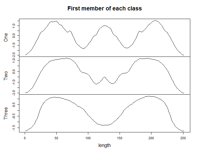
Figure 1: Profile of each Arrowhead class

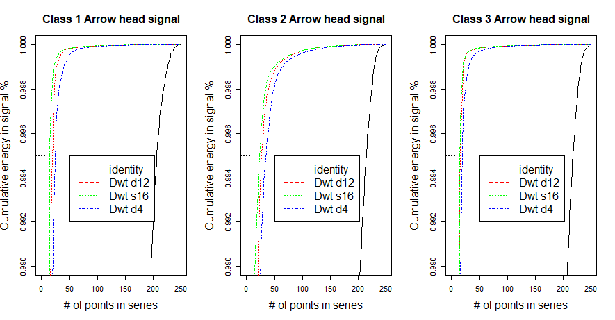
Figure 2: NPES of each Arrowhead Class using Wavelet Transforms

Following the $\mathbf{MWSCS}$ procedure, initially we applied various wavelet filters to each of the arrowhead classes to plot the NPES. Given the 251 data points in length, the wavelet transform deconstructing the signal to the first level, provided us with 125 detail and 125 smooth coefficients but also an “Extra” class of coefficients, how this class is calculated and implemented in the transform, by the chosen software is fully described in [8, Chap 4.11].

These additional coefficients are simply untransformed data. For this dataset as the “Extra” coefficients contain considerable signal energy/information, they are combined with the smooth coefficients in constructing our new data. For each transformed signal, the Extra coefficients contain an average of 1.41% of signal energy per transformed signal at level 1 and 3.45% at level 2.

The NPES of samples taken from each Arrowhead class highlight suitable wavelet filters to represent the energy in a smaller number of data points as shown in Figure 2. Little difference is apparent between the wavelet filters shown, however the filters s16 and d12 represent the energy slightly more efficiently than d4. Hence we use these wavelet filters to transform our signal data and build our transformed dataset, this however provides no compression in the signal representation as we will still have same number of wavelet coefficients as data points in the original signal.

By selecting only the smooth coefficients at the respective level we are able to reduce the number of attributes within our data and maintain classification accuracy as shown in Table 3. Here classification accuracy is defined as the number of correctly Classified Instances with respect to the dataset’s Class labels which are initially provided within the original data.

4.2.1 Arrowhead Results

Table 3 demonstrates the benefits of the wavelet transforms, s16 wavelet filter performs slightly better than d4 for the ensemble classifiers, The use of the smooth coefficients resulting from s16 (and when combined with d12), maintain accuracy while using reduced numbers of attributes.

Using the smooth wavelet coefficients and including the Extra coefficients, where these Extra coefficients contain considerable signal energy, still provide considerable accuracy, especially when using the ensemble classifiers.

• $\mathbf{Table\;\ref{tableArrow}\;Description:}$

• $\mathbf{Classifier}$ The first column is the list of classifiers used, see section 4.1

• $\mathbf{Raw\;data}$ results from classifying original data, being 251 units in length

• $\mathbf{Wavelet\;d4}$ results from data transformed using Wavelet filter d4, signal decomposed to four levels, 248 units in length

• $\mathbf{Wavelet\;s16}$ results from data transformed using using Wavelet filter s16, signal decomposed to four levels, 248 units in length

• $\mathbf{Wavelet\;s16\;\mathcal{S}_{1}+Extra}$ results from data transformed using s16 using only the smooth level 1 and Extra coefficients, 126 units in length

• $\mathbf{Wavelet\;s16\;d12\;combined\;\mathcal{S}_{2}}$ results from data transformed using s16 and d12 filters, combining the smooth level 2 coefficients from both transforms to form a new data series , 62 + 62 = 124 units in length. A MDWT, see section 2.1

• $\mathbf{Wavelet\;s16\;d12\;combined\;\mathcal{S}_{2}+Extras}$ results from data transformed using s16 and d12 wavelet filters, combining the smooth level 2 and Extra coefficients from both transforms to form a new data series , 64 + 64 = 128 units in length, again a MDWT.

Table 3: Classification of Arrowhead data, Cross Validation 10-Fold

	Classification Accuracy%
	Raw data	Wavelet d4	Wavelet s16	Wavelet s16	Waves s16 d12	Waves s16 d12
$\mathbf{Classifier}$		4 levels	4 levels	$\mathcal{S}_{1}$ + Extra	combined $\mathcal{S}_{2}$	comb. $\mathcal{S}_{2}$ + Extra
J48	75.35	76.03	74.41	79.14	77.72	72.72
Rforest	86.25	84.36	86.25	90.05	89.1	89.57
ForestPA	80.09	79.14	81.51	79.62	82.46	83.88
SysFor	82.46	81.52	81.99	83.41	84.36	84.36
SimpleCart	73.46	73.93	72.51	70.14	70.61	70.61

4.3 Mallat data

From the UCR dataset, Mallat Curve data, 8 distinct classes of 1024 units in length, see Figure 3. We combined the data, both testing and training sets to have a larger set containing 2400 records, eight classes of 300 records each.

Figure 3: Mallat data

Following the $\mathbf{MWCSC}$ procedure as with the Arrowhead data, using the NPES to determine suitable wavelets to represent the signal energy, we apply the classifiers to the wavelet transformed data. This time we use 20% of data for training and 80% for testing, (the actual records in these sets were chosen by WEKA).

4.3.1 Mallat data, Results

Table 4 highlights results from the Classifiers. The original data is 1024 unit long, hence the full wavelet transform also 1024 units long. Using the smooth wavelet coefficients from $\mathcal{S}_{1}$ results 512 units in length, similarly $\mathcal{S}_{2}$ results in 256 units and $\mathcal{S}_{3}$, 128 units.

Using the various levels of decomposition, increasing the effective compression of the signal transform we note that accuracy is maintained, especially with the ensemble classifiers. However when we combine the two $\mathcal{S}_{3}$ levels (a MDWT) from different wavelets (as determined by the NPES), then the ensemble classifiers maintain considerable accuracy, given the reduced transformed signal size, $\mathcal{S}_{3}\times$2 = 128 + 128 = 256 units. A small accuracy gain over the single wavelet transforms using $\mathcal{S}_{2}$ or $\mathcal{S}_{3}$.

Table 4: Classification of Mallat data, 20% training, 80% testing

	Classification Accuracy%
	Raw data	Wavelet s16	Wavelet s16	Wavelet s16	Wavelet s16	Waves s16 d8
$\mathbf{Classifier}$		10 levels	$\mathcal{S}_{1}$	$\mathcal{S}_{2}$	$\mathcal{S}_{3}$	combined S3
J48	98.88	94.48	97.29	95.99	95.67	94.74
Rforest	97.18	98.85	98.33	98.01	98.07	98.25
ForestPA	96.61	97.34	97.39	97.23	97.81	97.86
SysFor	95.52	95.93	96.15	94.63	95.15	95.36
SimpleCart	95.57	95.0	96.3	95.93	94.17	94.53

4.4 Ford data

From the UCR dataset, Ford data, 2 distinct classes of 500 units in length. here the classification problem is to diagnose whether a specific symption exists or not in an automotive subsystem. We use the original training and test sets as provided in the UCI data and follow the $\mathbf{MWCSC}$. The test set, had 681 records in one class and 629 in the other.

NPES determined wavelet filters d16 and s20 as suitable. Results in Table 5 show we may maintain accuracy even at higher levels of compression,(or attribute reduction). Using the smooth components at level 1, $\mathcal{S}_{1}$ results in 250 units, using $\mathcal{S}_{2}$ provides 125 units, $\mathcal{S}_{3}$ gives 62 units and $\mathcal{S}_{3}$ + Extra coefficient gives 63 units in length. Very little gain is evident in this last transform as only a minor levels of signal energy is contained within the Extra coefficients at the $3^{rd}$ level.

Table 5: Classification of Ford data, 3601 training records, 1320 testing records

	Classification Accuracy%
	Raw data	Wavelet d16	Wavelet d16	Wavelet d16	Waves d16 s20	Waves d16 s20
Classifier		S1	S2	S3	combined S3	comb. S3 + Extra
J48	56.13	58.03	56.44	52.42	58.71	58.18
Rforest	73.25	72.95	71.37	73.41	74.2	75.53
ForestPA	74.24	75.91	74.17	74.69	74.09	74.92
SysFor	62.27	59.17	59.59	63.79	64.47	60.38
SimpleCart	58.18	58.11	56.37	59.02	59.92	59.15

Remark 3

For the single tree method J48, It would appear that our choice of specific wavelets within the MDWT might not be crucial as no evidence of consistent additional gain between the two MDWT variations. However the choice of additional attributes (as provided by the MDWT) to train upon would seem to provide some minor gain over using a single Wavelet transform.

5 Conclusion

It has been shown previously that wavelets may be used for signal compression with little loss of accuracy [5]. Our MWCSC methodology which makes use of the NPES and MDWT provides us a method to determine suitable wavelets as well as add additional information to the attribute space. This enables us to use transformed data sets with smaller dimension than the original data yet still provide similar or enhanced accuracy. From the NPES graphic, Figure 2, we note that wavelet d4 is not as efficient at energy representation as wavelet s16, for the arrowhead dataset. This is similarly represented in Table 3 by comparing classification results, across the various classifiers of raw data as well as the data transformed by the d4 or the s16 wavelet filters.

Construction of the MDWT from suitable wavelets enhances the accuracy while offering an effective compressed representation of the signal to which the classifiers my be applied to. Inclusion of “Extra” coefficients into the construction of the MDWT, where such coefficients contain considerable signal energy adds additional accuracy for little extra computation, as they are an included class in the transform calculation where $\{X_{t}:t=1,\ldots,n\},\;n\neq 2^{J}\;J\in\mathbb{Z^{+}}.$

5.1 Future Work

Within the construction of a MDWT, each separate DWT used to decompose the time series had the level or scale $J_{0}$ of decomposition remain unchanged. This may not be optimal as wavelet family, filter length and scale of decomposition, may all be correlated with respect to how the energy/information in the signal is represented. Hence wavelet decomposition using different scales within a MDWT should be considered. The the number of wavelet filters within a MDWT might be altered depending upon importance of accuracy or compression (reduced number of attributes), in our experiment a MDWT consisted of only two different wavelet filters.

References

- [1] P. Grant and Md. Zahidul Islam :2019. A novel approach for noisy signal classification through the use of multiple wavelets and ensembles of classifiers. In R. Goebel, Y. Tanaka, & W. Wahlster (Eds.), 15th International Conference on Advanced Data Mining and Applications (ADMA 2019) (Vol. 11888, pp. 195-203). Springer. https://doi.org/10.1007/978-3-030-35231-8_14
- [2] P. Clark and T. Niblett: 1987. Induction in Noisy Domains. In Progress in Machine Learning (from the Proceedings of the 2nd European Working Session on Learning), 11-30, Bled, Yugoslavia: Sigma Press.
- [3] S, Fong, Using Hierarchical Time Series Clustering Algorithm and Wavelet Classifier for Biometric Voice Classification Journal of Biomedicine and Biotechnology Volume 2012, Article ID 215019.
- [4] Marco Grimaldi, Anil Kokaram, Pádraig Cunningham. 2002. Classifying Music by genre using wavelet packet transform and a round-robin ensemble, Comp Science Dept.; Electronic and Electrical Engineering Dept., Trinity College Dublin, Ireland.
- [5] Daoyuan Li, Tegawend´e F. Bissyand´e, Jacques Klein and Yves Le Traon. 2016. Time Series Classification with Discrete Wavelet Transformed Data: Insights from an Empirical Study, The 28th International Conference on Software Engineering and Knowledge Engineering.
- [6] Morteza Moazami-Goudarzi, Mohammad H. Moradi, Sara Abbasabadi, 2006. High Performance Method for Electrocardiogram Compression Using Two Dimensional Multiwavelet Transform, IEEE 7th Workshop on Multimedia Signal Processing.
- [7] A. Graps, 1995. An Introduction to Wavelets, IEEE Computational Science and Engineering Summer Vol 2, num 2.
- [8] D. B. Percival and A. T. Walden, 2000. Wavelet Methods for Time Series Analysis, Cambridge University Press.
- [9] G.P. Nason, 2008. Wavelet Methods in Statistics with R, Springer, New York.
- [10] R Core Team ,2013. R: A language and environment for statistical computing. R Foundation for Statistical Computing, Vienna, Austria. URL http://www.R- project.org/.
- [11] W. Constantine and D. Percival, 2017. wmtsa: Wavelet Methods for Time Series Analysis. R package version 2.0-3 http://CRAN.R-project.org/package = wmtsa.
- [12] Eibe Frank, Mark A. Hall, and Ian H. Witten, 2016. The WEKA Workbench. Online Appendix for “Data Mining: Practical Machine Learning Tools and Techniques”, Morgan Kaufmann, Fourth Edition.
- [13] Y. Chen, E. Keogh, B. Hu, N. Begum, A. Bagnall, A. Mueen, and G. Batista, “The ucr time series classification archive,” October 2018, https://www.cs.ucr.edu/ eamonn/time_series_data_2018
- [14] R. Quinlan, 1993. C4.5: Programs for Machine Learning. Morgan Kaufmann Publishers, San Mateo, CA.
- [15] L. Breiman, Machine Learning (2001) 45:5. https://doi.org/10.1023/A:1010933404324
- [16] Md Nasim Adnan, Md Zahidul Islam. 2017. Forest PA: Constructing a decision forest by penalizing attributes used in previous trees. Expert Systems With Applications. 89:389-403.
- [17] Md Zahidul Islam and H. Giggins, 2011. Knowledge Discovery through SysFor: A Systematically Developed Forest of Multiple Decision Trees, In Proc. of the Ninth Australasian Data Mining Conference (AusDM 11).
- [18] Leo Breiman, Jerome H. Friedman, Richard A. Olshen, Charles J.Stone, 1984. Classification and regression trees Boca Raton : CRC Press.