Julia for Biologists

Elisabeth Roesch, Joe G. Greener, Adam L. MacLean, Huda Nassar, Christopher Rackauckas, Timothy E. Holy, Michael P.H. Stumpf*

Increasing emphasis on data and quantitative methods in the biomedical sciences is making biological research more computational. Collecting, curating, processing, and analysing large genomic and imaging data sets poses major computational challenges, as does simulating larger and more realistic models in systems biology. Here we discuss how a relative newcomer among computer programming languages – Julia – is poised to meet the current and emerging demands in the computational biosciences, and beyond. Speed, flexibility, a thriving package ecosystem, and readability are major factors that make high-performance computing and data analysis available to an unprecedented degree to “gifted amateurs”. We highlight how Julia’s design is already enabling new ways of analysing biological data and systems, and we provide a, necessarily incomplete, list of resources that can facilitate the transition into the Julian way of computing.

C omputers are tools. Like pipettes or centrifuges, they allow us to perform tasks more quickly or efficiently; and like microscopes, NMR or mass-spectrometers, they allow us to gain new, more detailed insights into biological systems and data. Computers also allow us to define, simulate and test mathematical models of biology. As computational power evolved, solving biological problems computationally became possible, then popular, and eventually, necessary [1]. Entire fields such as computational biology and bioinformatics emerged. Without computers, the reconstruction of structures from X-ray crystallography, NMR, or cryo-EM methods would be impossible. The same goes for the genome project [2], which used computer programs to assemble and analyze the DNA sequences generated; and, to this day, computer programs continue to enable new science by analyzing data from the genome project. More recently, vaccine development has benefited immensely from recent advances in algorithms, software, and computer hardware [3].

Programming languages are also tools. They provide the bridge between hypothesis or model formulation and computational power. Programming languages make it possible to instruct computers to run algorithms, for example for the analysis of biological data. Some languages are very good at specific tasks – think Perl for string processing tasks; or R for statistics and data analysis – whereas others – including C, C++, and Python – have been used with success across many different domains. In biomedical research the prevailing languages have arguably been R [4] and Python [5]. Much of the high-performance backbone supporting computationally intensive research, hidden from most users, however, continues to rely on C/C++ or Fortran. Many computationally intensive studies are designed in a way where an initial first draft is coded in R, Python or Matlab (first language), and subsequently translated into C/C++ or Fortran (second language) for performance reasons. This is known as the two-language problem.

While this two-language approach has effectively facilitated and sped up scientific discovery in many instances, one can imagine instances where this model has been limiting. When moving a certain implementation from one programming language to a second, faster, programming language, straightforward “verbatim" translation may not be the optimal route: the faster language (such as C/C++ or Fortran) often provides the programmer with a much higher margin of autonomy, such as the ability to choose how memory is accessed or allocated or to employ slightly more sophisticated data structures [6]. Exploiting these gains may require a complete rewrite of the algorithm [7, 8] to ensure faster implementations, faster scaling, or potentially better packaged code. This requires expertise across both languages, but also rigorous testing of the code in both languages.

Figure 1: Julia is a tool for the biologist to discover new science. In the biological sciences, the most obvious alternative to the programming language Julia is R, Python or Matlab. Here, we contrast the two potential pathways to new biology with a mountaineering excursion: The top of the mountain represents "New Biology". There are two potential base camps for the ascent: Base camp 1 (left, red) is "R/Python/Matlab". Base camp 2 (right, green) is "Julia". To get to the top, the mountaineer – representing the biologist – needs to overcome certain obstacles such as a glacier and a chasm. They represent research hurdles such as large and diverse data sets or complex models. Starting at the "Julia" base camp, the mountaineer has access to efficient and effective tools such as a bridge over the glacier and a rocket to simple fly over the chasm. They represent Julia’s top three language design features: Abstraction, speed and metaprogramming. With these tools, the journey to the top of the mountain becomes much easier for the excursionist. In other words, Julia allows the biologist to not be hold back by problems such as the "Two-language problem" and the "Expression problem" and therefore Julia helps the biologist to discover new science.

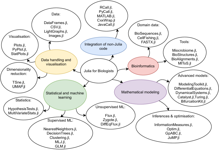
Figure 4: An overview of Julia’s package ecosystem presented by topic groups.

1. Language design	• Julia is user friendly. $\rightarrow$ It is easy to code. • Julia is a high performance language. $\rightarrow$ It is fast. • Julia offers a high level of abstraction. $\rightarrow$ It is flexible. • Julia can be used for metaprogramming. $\rightarrow$ It can code automatically. • Julia is not only good in one area but in many. $\rightarrow$ It enables "one language" projects.
2. Low barrier to entry	• Easy to learn due to intuitive semantic and easy to read syntax. • Accessible via various interfaces, REPL, IDE, or Jupyter notebook. • Existing non-Julia code can be easily integrated into new Julia projects via language specific packages (Figure 4, Integration of non-Julia code).
3. Additional reasons	• Julia is free, open-source and hosted on GitHub. • Julia offers (generally) excellent documentation, tutorials, and help available directly from active and welcoming community members via various communication channels such as Slack, Discourse, Twitter or Zulip. • Julia’s package ecosystem provides functionality for a wide range of oft-performed tasks in computational biology research (Figure 4, Table 2). • Julia code is smoothly extendable which enables and encourages easy contributions and collaborations to/with existing projects, as well as writing, integrating and sharing new, user specific packages.

Table 1: As Julia is a relatively young language, it is save to assume that the majority of biologists are not using Julia yet. In this table we present arguments that make Julia a good programming language for biologists.

As the field of computational biology evolves, the two-language approach is still surprisingly persistent: higher-level languages (R, Python) are used for algorithm development and preliminary analyses. The better performing languages (C/C++, Fortran, or CUDA) are used in specific instances and with considerable additional effort if the computational burden becomes overwhelming. This is questionable from an efficiency perspective but also problematic in regards to the correctness and accuracy as the translation step leaves room for mistakes and misinterpretation; especially if the translation is done by someone who is not a domain expert [9]. This issue will only become more problematic as the demand for high performance code with good scalability continues to increase to meet the demands of bigger data sets and more detailed models. However, this also makes it very evident, that the accessibility and ease-of-use aspect of the programming language is of considerable importance to biomedical scientists, and, implicitly, the progress of biomedical research.

Julia [10] is a relatively new programming language, and the main advantage for biologists is that it challenges the two-language concept, by being a language that “looks like Python and runs like C". Users do not have to choose between ease-of-use and high performance – Julia is built to be easy to program in and fast [11]. This and the growing ecosystem of state-of-the-art application packages and introductions [8, 12] make it an attractive choice for biologists.

Biological systems and data are multifaceted by nature, and to describe them, or model them mathematically, requires flexibility of a programming language to handle of connect different types of highly structured data, see Figure 1. There are three hallmarks of the language which make it particularly suitable to meet the current and emerging demands of biomedical scientists that we discuss here in some detail: speed, abstraction and metaprogramming. We discuss each language feature and its biological relevance in the context of concrete examples. And we provide a basic toolset and tips to get started with Julia, see Table 1. Further supporting online material as well as code examples are provided in github.com/ElisabethRoesch/Perspective_Julia_for_ Biologists.

Speed

The speed of a programming language is not just a matter of convenience that allows us, for example, to finish analyses more quickly; it also enables new science and better science. Speed is important when analysing large data sets [13, 14] that are becoming the norm in many areas of biology [15]. Slow operations might not hinder scientific discovery when performed a small number of times. However, when performed repeatedly on large data set, the speed of a programming language can become the limiting factor for new discoveries (See: Speed Example 1). Similarly, simulating large and complex computational models is only possible with fast implementations (See Speed Example 2); and digital twins [16, 17] in precision medicine are useless without fast and convenient computation.

The speed of the programming language also determines how extensively we can test statistical analysis or simulation algorithms before using them on real data. Thorough testing of a new statistical algorithm can be expected to be around 2-3 orders of magnitude more costly in computational terms than a single “production run" [14]. Furthermore, the quality of approximations also depends on many factors (e.g. number of tested candidates [18, 19] and grid step sizes [20]) and faster code enables better analysis.

In the following we use two examples of Julia in Biology to highlight some of Julia’s speed features and showcase how they enable new biology. We also provide some technical insights into the design features underlying Julia’s speed [21].

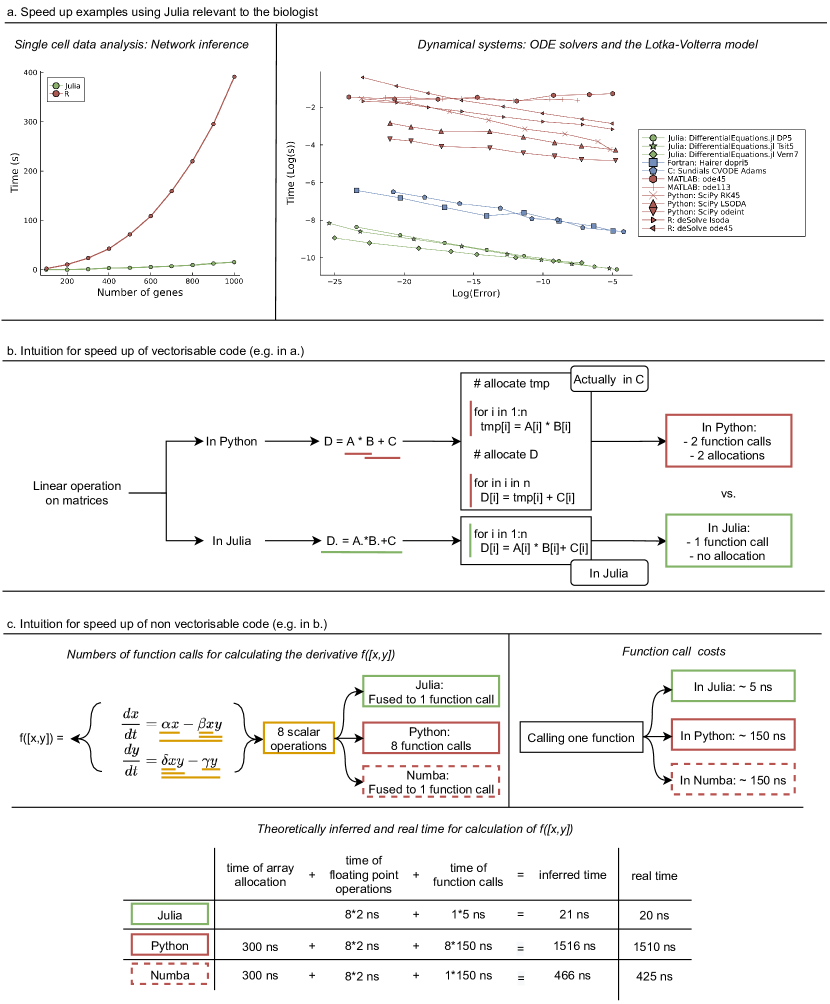
Figure 2: Julia’s speed feature. (a) Examples relevant to the biologist. Left: Time to calculate mutual information for all possible pairs of genes of a single cell data [14]. Right: Benchmark of ODE solvers (More systems in [22]). (b) Illustration of speed-up of vectorisable code (as in (a)). (c) Intuition for speed up of non vectorisable code (as in b).

Example 1: Fast Network Inference from Single Cell Data.

In single cell biology, we can now measure the expression levels of tens of thousands of genes in tens of thousands of cells. Increasingly we are even able to do this with high spatial (that is sub-cellular) resolution [23]. But searching for patterns in complex and large data-sets can be computationally expensive: even apparently simple tasks, such as calculating the mutual information (MI) [24] across all pairs of genes in a large data set can quickly become impossible.

The inference of gene regulatory networks (GRN) from single cell data is a statistically demanding task, and one where Julia’s speed can help. This is illustrated by the analysis of Chan et al. [14] where information theoretical measures were used to infer GRNs from transcriptomic single cell data of qPCR experiments on megakaryocyte-erythroid progenitor cells during human hematopoiesis [25], early embryonic development [26], and embryonic hematopoietic development [27]. The MI has to be calculated for gene pairs; but a multivariate information measure, partial information decompositio (PIDC) is also considered to separate out direct and indirect interactions [24], and this requires looking at all gene triplets [28].

The run-time of algorithms implemented in the Julia package InformationMeasures.jl can be compared to the popular R package minet [29] for different number of genes and numbers of cells (Figure 2(a) left). For small numbers of genes, differences are significant but not prohibitive: inferring a network with 100 genes takes around 0.3 seconds in Julia compared to 1.5 seconds in R; but already for 1,000 genes the inference times differ substantially: 17 seconds in Julia and 390 seconds ($>$20-fold difference) in R; for – by today’s standards small – datasets with 3,500 genes and 600 cells R needs over 2.5 hours, compared to Julia’s 134 seconds ($\approx$ 64-fold difference); and in real-world applications [28] 400-fold speed differences are possible. Here we are reaching the threshold of what can be tested and evaluated rigorously in many highlevel languages. Overall, multivariate information measures would almost certainly be unfeasible in pure R or Python implementations.

The reason for this performance difference is Julia’s ability to optimize “vectorizable” code; cf. Figure 2(b) [21]. Users of languages like Python and R are familiar with vectorized functions, such as maps and element-wise operations. Julia gains further performance improvements by combining its Just-in-Time (JIT) compilation with vectorized functions via a trick known as operator fusion. When writing a chain of vector expressions, like $D=A*B+C$ (where $A,B,C$ and $D$ and $n$-dimensional vectors), libraries like NumPy call optimized code that works under the hood, and which is generally written in another, faster language like C/C++, and these operations are computed sequentially. For this example, $A*B$, C code is called to produce a temporary array, $tmp$, and then $tmp+C$ is again evaluated using C code to produce the desired $D$. Allocating the memory for the temporary intermediate, $tmp$, and the final result $D$ is $O(n)$ (which means that the time it takes to complete the computation increases with approximately with $n$, the length of the vectors), and scales proportionally to the compute cost; thus no matter what the size of the vectorization is, there is a major unavoidable overhead. Julia uses the “.” operator to signify element-wise action of a function, and therefore the equation can be written as $D.=A.*B.+C$. When the Julia compiler sees this, so-called broadcast, expression it fuses all nearby dot-operations into a single function, and JIT compiles this function into a loop. In concrete terms, NumPy makes two function calls and spends time generating two arrays, whereas Julia makes a single function call and reuses existing memory. This and similar performance features are now leading package authors of statistical and data science libraries to recommend calling into Julia for such operations, such as the recommendation by the principal author of the R lme4 linear mixed effects library to use JuliaCall to access MixedModels.jl in Julia (both written by the same author) for an approximately 200x acceleration[30].

Example 2: Accelerating Dynamical Systems Modeling in Systems Biology and Pharmacology.

Systems biology and related fields, including quantitative systems pharmacology (QSP), are also benefitting from Julia’s speed. Modeling and simulation are transforming the drug discovery pipeline, lowering the risk of failed trials, and allowing efficiency gains in drug development and substantial financial savings in the drug development process [31]. However, even with these successes most trials do not undergo in-depth preclinical analysis. The major reason why is time: any delay in the start of the clinical trial increases the overall cost. Improvements in QSP can remedy this situation.

Solving large systems of ordinary differential equations (ODEs) (and increasingly also stochastic dynamical systems) lies at the core of these modelling studies. We typically have nonlinear functions, $f$, and solving them in high-level languages such as R, Python or Matlab can be slow. Therefore solver libraries are often written in a faster language, such as C/C++ or Fortran. The limiting factor then is the user’s non-linear set of equations, $f$. In languages like Python or R, there is a high function call overhead: every operation that is called is more expensive than in a fast language (approximately 150-350ns per call [32] while the function calls can take approximately 5ns in Julia or C). Scalar operations, like evaluating a Hill kinetic function $[A]^{\prime}=\frac{[B]^{n}}{\omega+[B]^{n}}$, can take microseconds instead of nanoseconds, see Figure 2. “Vectorization”, as recommended in languages such as Python or R, packs more floating point operations into each C function call and can help to speed this up somewhat. Even accelerators like Numba still require a context change from Python to the compiled C function, which can hamper performance, especially for sparse reaction networks. Furthermore, vectorization requires a certain level of regularity and simplicity in the equations, and the nonlinear systems typically found in biology can be anything but simple; therefore traditional interpreted languages will always tend to perform poorly for nonlinear models.

When solving an ODE, the function $f$ is called thousands or millions of times, exacerbating this difference. Figure 2 showcases some examples of biological models where such simulations are 50x-400x faster than those using leading packages in R and Python. In a typical preclinical drug development pipeline this has led to 175-fold acceleration of QSP model analysis once the model had been translated from a combination of MATLAB and C code into Julia [33]. Julia’s speed enables more efficient clinical trial analyses and its libraries have been shown to be even faster than commonly used Fortran libraries in this domain of ODE modeling [34].

Abstraction

Compared to other programming languages such as R and Python, or C/C++ and Fortran, Julia allows an exceptionally high level of abstraction[35]. In order to highlight the advantages of an abstract programming language[36], we can use an analogy to a more standard tool of a biologist – a pipettor – to develop some intuition for the important role of abstraction.

The pipettor is a standard piece of lab equipment made with slightly different designs by different manufacturers; nevertheless they all perform the same task in a similar way. It thus takes minimum effort to get used to a new pipettor, without having to retrain on every aspect of an experimental protocol. Abstraction achieves the same for a software. Similar to the described abstract interface “pipettor”, in Julia we have interfaces such as the AbstractArray interface. All implementations of it are “array-like” structures and provide the same core functionalities which an “array-like” structure is expected to have. This allows us to easily swap between different implementations of the same interface and hence promotes specification without the often feared loss of the ability to integrate with existing software or adapt to new applications[37].

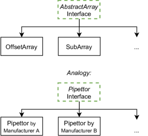
Figure 3: Interfaces: Pipettors and the AbstractArray.

Compared to, e.g., physics, the biological sciences have a high level of heterogeneity in the prevalent data [38, 39, 40]. This poses challenges for programming languages[37] and data analysis pipelines, and changes to data may require substantial rewriting of code for processing and analysis. We may end up with different implementations of algorithms for different types of data; or we may remove details and nuance from the data to enable analysis by existing algorithms. With abstraction we do not have to make such choices. Julia’s abstraction capabilities provide room for both specialisation and generalisation through features such as abstract interfaces and generic functions that can exploit the advantages of unique data formats with varying internal characteristics without an overall performance penalty.

Community	Topic	Example packages
JuliaData	Data manipulation, storage, and I/O	DataFrames.jl, JuliaDB.jl, DataFramesMeta.jl, CSV.jl
JuliaPlots	Data visualization	Plots.jl, Makie.jl, StatsPlots.jl, PlotlyJS.jl
JuliaStats	Statistics and Machine Learning	Distributions.jl, GLM.jl, StatsBase.jl, Distances.jl, MixedModels.jl, TimeSeries.jl, Clustering.jl, MultivariateStats.jl, HypothesisTests.jl.
BioJulia	Bioinformatics and Computational Biology	BioSequences.jl, BioStructures.jl, BioAlignments.jl, FASTX.jl, Microbiome.jl
JuliaImages	Image processing	Images.jl, ImageSegmentation.jl, ImageTransformations.jl, ImageView.jl
EcoJulia	Ecological research	SpatialEcology.jl, EcologicalNetworks.jl, Phylo.jl, Diversity.jl
SciML	Scientific machine learning	DifferentialEquations.jl, ModelingToolkit.jl, DiffEqFlux.jl, Catalyst.jl
FluxML	Machine Learning	Flux.jl, Zygote.jl, MacroTools.jl, GeometricFlux.jl, Metalhead.jl

Table 2: Julia provides a rich package ecosystem for biologists. Related packages are organised in package communities. In this table, we present an overview of package communities we consider most relevant to biologists.

Example 1: Structural bioinformatics with composable packages.

The flexibility of Julia means that packages from different authors can generally be combined easily into workflows, a feature known as composability. Users can benefit from Julia’s flexibility just as much as package developers. For example, we consider a standard structural bioinformatics workflow, where we want to download and read the structure of the protein crambin from the Protein Data Bank (PDB). This can be done using the BioStructures.jl package [41] from the BioJulia organisation, which provides the essential bioinformatics infrastructure. Protein structures can be viewed using Bio3DView.jl, which uses the 3Dmol.js JavaScript library [42] as Julia can easily connect to packages from other languages. We can show the distance map of the C atoms using Plots.jl; while Plots.jl is not aware of this custom type, a Plots.jl recipe makes this straightforward. BioSequences.jl provides custom data types of sequences and allow us to represent the protein sequence efficiently. With this BioAlignments.jl can be used to align our sequences of interest. This suite of packages can be used to carry out single cell full-length total RNA sequencing analysis [43] quickly and with ease. A few lines of code in BioStructures.jl allow us to define the residue contact graph using LightGraphs.jl, giving access to all the optimised graph operations implemented in LightGraphs.jl for further analysis, such as calculating the betweenness centrality of the nodes. If the code is written in Pluto.jl, then updating one section updates the whole workflow, which is essential for exploratory analysis.

Packages can be combined to meet the specific needs of each study; for example to generate protein ensembles and predict allosteric sites [44], or to carry out information theoretical comparisons using the MIToS.jl package [45].

In this example we have used at least five different packages together seamlessly. Plots.jl, BioAlignments.jl and LightGraphs.jl do not depend on, or know about BioStructures.jl but can still be used productively alongside it. Abstraction means that the improvements in any of these packages will benefit users of BioStructures.jl, despite these packages not being developed with protein structures in mind.

This level of package composability is common across the Julia ecosystem and is ultimately enabled by abstract interfaces supported by multiple dispatch, i.e. the ability to define multiple versions of the same function with different argument types. Programmers can define standard functions such as addition and multiplication for their own types, which means that functions in unrelated packages often "just work" despite knowing nothing about the custom types. This is rarely seen in languages such as Python, R and C/C++, where the behaviour of an object is confined to one place [36] and combining classes and functions from different projects requires much more (of what is known as) “boilerplate" code. For example, the popular Biopython project [46] has grown over many years to become a powerful package covering much of bioinformatics. But extensions to Biopython objects are generally added to (an increasingly monolithic) Biopython, rather than existing in independent packages. This can lead to objects and algorithms that have the difficult task of fitting all use cases simultaneously [47]; this can introduce reservations about adding code that interacts with other packages and/or increases dependencies.

By comparison, the composability of Julia, which is connected to the underlying technical feature of multiple dispatch, enables scientists to combine packages to carry out new tasks in ways probably never imagined by the creators of Julia [48]. Composability also facilitates writing generic code that can be used beyond its intended application domain. For example, Tables.jl provides a common interface for tabular data, allowing generic code for common tasks on tables; currently, some 129 distinct packages draw on this common core for purposes far beyond the initially conceived application scope.

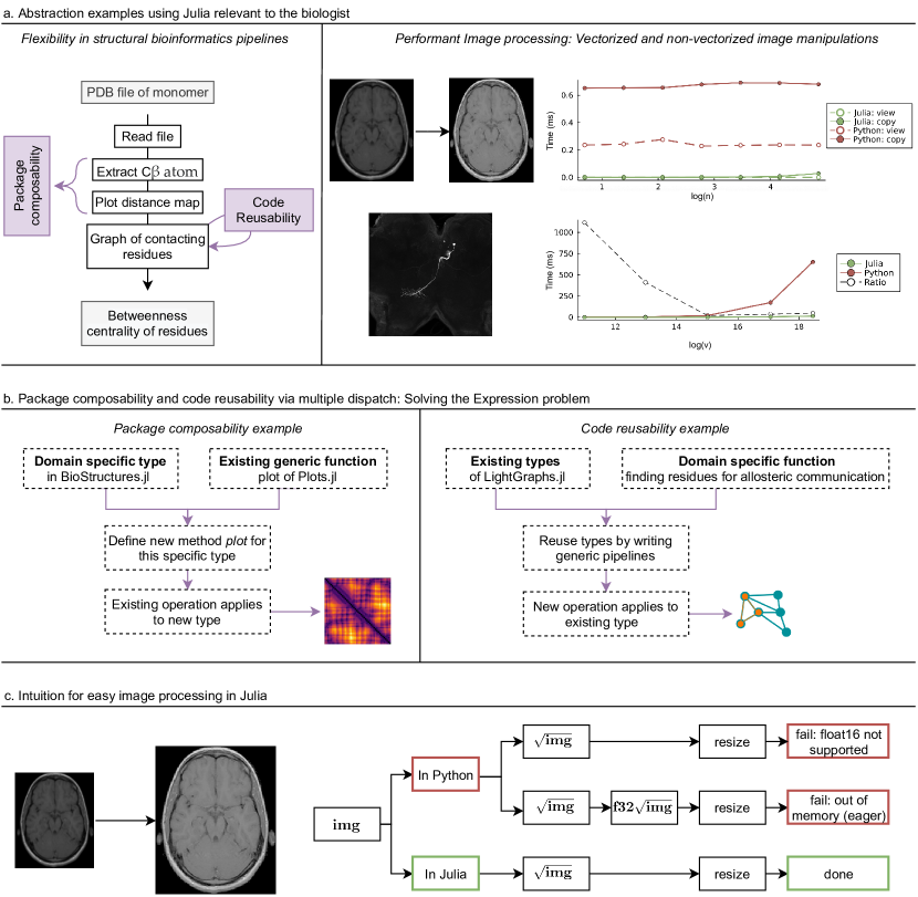
Figure 5: Julia’s abstraction feature. (a) Two examples relevant to the biologist. Left: Package composability and code reusability in structual bioinformatics pipelines. Right: Contrasting (top) and segmenting (bottom) images as examples for high performance vectorizable and non-vectorizable image manipulations in Julia. (b) Conceptual background of package composability and code reusability in structual bioinformatics pipeline: Julia solving the expression problem as it enables an easy addition of types and functionalities without causing compatibility issues with existing code. (c) Intuition for robustness of image processing in Julia vs. Python.

Example 2: Flexibility and performance in image processing.

Microscopy in its many forms underlies much of modern biology. But extracting information from imaging data is challenging for two main reasons. The first challenge lies in the nature of the raw data. Scientific images can be very large, and it is not uncommon for datasets to reach a size of multiple terabytes [49, 50]. In such instances, initially minor performance inconveniences can quickly extrapolate to become limiting factors for scientific discovery. Also, the images – typically internally represented as arrays – often exhibit great diversity: for example, a single imaging dataset may have two or three spatial dimensions, zero or one temporal dimensions, and a color- or modality-channel. This is further exacerbated by the complexity of the accompanying meta information on the imaging conditions and technologies which also influence down stream analysis and interpretation. Having the flexibility to accommodate for this level of diversity whilst also providing the necessary performance needed when dealing with data of this size, is a non-trivial challenge for any programming language with significant implications for outcomes [51, 52].

The second reason for carefully thinking about the choice of software for image processing pipelines, lies in the nature of processing pipelines themselves. Typically the data are sequentially manipulated over multiple steps. In a naive approach, a new, slightly altered version of the large raw dataset is created and stored for each step in the pipeline. This is inherently inefficient and becomes quickly infeasible or impossible as data sizes grow beyond storage capacities. Documenting and tracking different combinations of data manipulation steps is also non-trivial as each step could lose information.

Efficient data representation combined with flexible processing is of essence to extract meaningful conclusions from the data. Abstraction is Julia’s key feature that enables state-of-the-art image processing [53, 54]: by keeping a high level of abstraction in the internal data representations, the diversity in image data can be captured and exploited, and modifications to the data become easier, too. A core component for implementing the relevant abstraction in Julia is provided by the AbstractArray interface [55], especially in its combination with lazy operations. In a normal, “eager”, operation, each computation is executed immediately upon being invoked. By contrast, lazy operations delay their computations until the latest possible moment in time, i.e. the execution is separated from the declaration of a computation. In some cases, this can be delayed all the way to the moment where we wish to visualize the processed data, so that no computation needs to occur on any data not being inspected.

As previously described, the AbstractArray interface can be thought of as a template which creates an agreement between existing software and the user’s software. We can use the template, i.e. implement the AbstractArray interface, in order to define a new array type which optimally fits their data format. By using the interface, we also agree to provide certain functionalities for this new object. Providing both high levels of customization and standardization of operations that need to be supported by an array-like object, allows for the composition of complex and highly specialised pipelines. The specifics of the array no longer matter because of the abstraction. Many AbstractArray interface implementations helpful in image processing already exist and we do not have to start from scratch for each new imaging modality. Examples include SubArrays (region-of-interest “view" selection), MappedArrays (lazy-modification of values), “ReshapedArrays” (lazy-modification of dimensionality), and WarpedViews in the ImageTransformations.jl package (lazy coordinate transformations).

With effective lazy operations, it becomes possible to manipulate and inspect massive data sets even with relatively modest computing hardware, because the hardware only needs to load, process, and display the small subset of the data being actively explored. Pre-processing stages that might require tuning several parameters to the particulars of the data set can be refined quickly, with each iteration perhaps comprising only a few seconds or minutes, rather than the hours, days, or weeks that might be required if each step had to cached to disk between manipulations.

Other languages support the concepts of abstraction and lazy operations, too, but despite considerable investment they do not provide the same level of comfort and capability available in Julia. For example, in Python, the most widely-used lazy-operation package is Dask [56], which has a sophisticated engine for managing computational graphs and applying them across distributed data sets. However, when using Dask to process large image data sets, one frequently encounters severe limitations on composability (Figure 5(c)): some algorithms may not support outputs of previous stages, while others may force an eager intermediate step in the pipeline potentially exhausting memory resources, and yet others may attempt to allocate an unachievable output array. By contrast, with Julia, one can routinely expect that arbitrary combinations of processing "just work" together, and we can use lazy operations along the whole image processing pipeline. Because Julia aggressively optimizes computations at a granular level (all the way to the single pixel), this flexibility comes with little or no overhead, in marked contrast to languages such as Python (Figure 5(a) and additional information in the accompanying Git repository).

Metaprogramming

As our knowledge of the complexities of biological systems grows ever deeper, so does our need of means to simplify the construction and analysis of mathematical models of these systems. Currently, most modeling studies in biology rely on programming languages that treat source code as static: once written, it can be processed into loaded and executing code, but it is never changed during execution of the program. We can compare this linear control process to the central dogma of biology [57, 58]: Source code (DNA) is transformed into loaded code (RNA), and executing code (protein). In fact, we know now that this process (DNA$\longrightarrow$RNA$\longrightarrow$Protein) is not linear at all: for example, RNA and proteins can alter how and when DNA is translated. Programming languages that support metaprogramming break the linear flow of the computer program in a similar manner to the analogy of the central dogma. With metaprogramming, source code can be written that is processed into loaded and executing code and it can also affect the source code. This shifts our perception of code to that of a dynamic instance. By treating code as part of the data, we can write computer code that changes code: the program can modify aspects of itself during run-time (Figure 6(a)).

Metaprogramming enables a form of reflection and learning by the software and the concept originated in early artificial intelligence research, in particular in the context of the LISP programming language. Of course, the ability of a program to modify computer code needs to be channelled very carefully. In Julia, this is done via a feature called hygenic macros [59]. These are flexible code templates, specified in the program, and which can be manipulated at execution time. They are called "hygenic" because they prohibit accidentally using variable names (and thus memory locations) that are defined and used elsewhere. These macros can be used to generate repetitive code efficiently and effectively.

But there are other uses that can enable new research. Perhaps this is most immediately relevant for modelling biological systems. Unlike in physics, first principles (conservation of energy, momentum, etc., and their related symmetry relationships [60]) offer little guidance as to how we should construct models of biological processes and systems. For these notoriously complicated biological systems, trial and error, coupled to biological domain expertise, and state-of-the-art statistical model selection are required at a very minimum [61]. Great manual effort is spent on the formulation of mathematical models, the exploration of their behavior, and their adaptation in light of comparisons to data and/or design principles. Metaprogramming, or the abilities of introspection and reflection during runtime [59], and the ability to automate these parts of the modeling process open up wide scope for new approaches to modeling biological systems (Figure 6(b)).

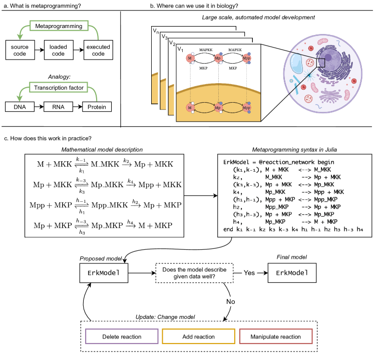
Figure 6: Julia’s Metaprogramming feature. (a) Illustration of metaprogramming and an analogy the the central dogma of molecular biology. (b) Application area of metagprogramming in biology. (c) Example workflow.

Example 1: Biochemical reaction networks.

Mathematical models of biochemical reaction networks allow us to analyze biological processes and make sense of the bewilderingly complex systems underlying cellular function [62, 63, 64]. But the specification of mathematical models is challenging and requires us to specify all of our assumptions explicitly. We then have to solve these models based on assumptions about the dynamics. Solving a given reaction networks can involve solution, for example, of ordinary differential equations (ODEs), delay differential equations, stochastic differential equations (SDEs), or discrete-time stochastic processes. To create instances of each of these models would typically – in languages such as C/C++ or Python – require writing different snippets of code for each modelling framework. In Julia, via metaprogamming, many different models can be generated automatically from a single block of code. This simplify workflows and make them more efficient, but also removes the possibility of errors due to model inconsistencies. Good programming tends to be lazy, and the lazyness enabled by metaprogramming reduces the risk of introducing errors into code.

For example, the ERK phosphorylation process shown in Figure 6(b)[65]. Here ERK is doubly phosoporylated (by its cogniscant kinase, MEK) and dephosphorylated by a phosphatase upon which it can shuttle into the nucleus and initiate changes in gene expression. It is a small and important component of a larger signalling network. Its role has made ERK a target of extensive and intensive analysis, and modelling has helped to shed light on its function and role in cell-fate decision making systems [66]. This small system – albeit one of great importance and subtlety – forms a building blocks for larger, more realistic biochemical reaction [62] and signal transduction [67] models.

In Julia, using Catalyst.jl [68], this model can be written directly in terms of its reactions, with the corresponding rates {$k_{1},k_{2},k_{3}$}: source code is human readable and differs minimally from the conventional chemical reaction systems shown in Figure 6(c).

The science is encapsulated in this little snippet and solving of the reaction systems then proceeds by calling the appropriate simulation tool from DifferentialEquations.jl: for a deterministic model specified the reaction network is directly converted into a system of ODEs (via ODESystem). Likewise, the same reaction network can be directly converted into a model that is specified by SDEs (via SDEProblem) or a discrete-time stochastic process model (via DiscreteProblem). Each of these cases leads to the creation of a distinct model that can be simulated or analyzed; yet all of the models share the underlying structure of the same reaction network. To simulate one of the resulting models, the user needs to specify only the necessary assumptions required for a simulation – i.e. the parameter values and initial conditions – as well as any further assumptions required that are specific to the model type, e.g. the choice of noise model for a system of SDEs. Adapting the model to include nuclear shuttling [69] of Erk as in Figure 6(c), or extrinsic noise upstream of Erk [65] is easily achieved in the metaprogramming approach.

Fitting models to data, or estimating their parameters from data, is also supported by the Julia package ecosystem. Parameter estimation by optimsing the likelihood, posterior or a cost-function is straightforward using the Optim.jl [70] or JuMP.jl [71] packages. And because of Julia’s speed it has become much easier to deploy Bayesian inference methods; here, too, metaprogramming helps tools such as the probabilistic programming environment, Turing.jl [72]. Approximate Bayesian computation approaches are already implemented in Julia in the package GpABC.jl [18]; they also benefit from Julia’s combination of speed, abstraction and metaprogramming, and are faster than implementations in other languages (including some of the authors’ work [73]).

Example 2: Whole cell modeling.

An additional application area for metaprogramming is the development of physiologically more realistic models, whether at the levels of whole cells, tissues, or even the physiology of whole organisms. In whole cell modeling, models potentially scale up to the size of $10^{3}-10^{5}$ species [74] and a key problem is that constructing models of this size is extremely difficult [75, 76]. In fact even small parts of such models, see Figure 6, such as signalling cascades have a large number of (generally unknown) parameters. Here model development cannot rely on manual curation or inspired guesswork [75]. Instead automated model development will be required [74]. The reasons for this is that the bookkeeping efforts required to keep track of molecular species, their interactions, and the ways in which molecule numbers change as a result of biochemical interactions, are simply not manageable by conventional means. We do not know the model structure and therefore have to experiment with different model-setups. Without metaprogramming we would have to write or adapt the cellular simulation code for each new attempt. Plus, of course, nobody is able to check the validity of such a large model in the way we can check a simple mathematical model of the type that has traditionally dominated theoretical biology.

Developing a whole cell model will almost certainly involve piecing together sub-models, for which we can build on Catalyst.jl. Calibrating such (sub-) models against data – that is to infer parameters from data – is a demanding task, that has yet to be solved for such large systems (it is a priori not clear to what extent this can be solved). Approximations to the dynamics and/or the inference process can help; and for many sufficiently small systems (say signalling networks) current tools will allow us to determine their parameters from literature and/or data, as described in the example above. We may, in addition, want to use efficient approximations to the stochastic dynamics [77, 78], such as provided by MomentClosures.jl [79]. This can be coupled to parameter inference, as described above, via optimization (Jump.jl [71]) or Bayesian inference (Turing.jl [72] and GpABC.jl [18]).

Catlab.jl is a package that makes composing and combining smaller models into a larger model possible, and relatively straightforward. The toolset that we can use to construct such models continues to grow. For example, hypergraphs provide a much more flexible representation for mathematical models that conventional networks, and For such comprehensive models, grown in a principled way, the SciML suite, via e.g. DiffEqSensitivity.jl [80], allows us to quantity uncertainty and assess sensitivity of model outputs both locally and globally. Metaprogramming alleviates the need to "hard-code" such large models. Instead they can be generated automatically without sacrificing the runtime efficiency of the simulation models.

The model development process enabled by the pipeline, Sub-model formulation $\longrightarrow$ Sub-model fitting $\longrightarrow$ Composition of Large Model from Sub-models $\longrightarrow$ Sensitivity and Uncertainty Analysis, differs from the way in which the first (and so far only) comprehensive whole cell model was generated, which relied on a lot of manual and expert intervention and input [81], which will not scale to other organisms [74].

Overall, metaprogramming in Julia enables the automated construction of models of all sizes: from small biochemical reaction network models to whole cell models. Simulation, inference, and analysis of these models can all be performed with great paucity of code, reducing opportunities for errors to arise, and greatly enhancing our ability to describe and predict complex biological processes with mathematical models.

Outlook

When choosing a programming language we have many choices, but they all boil down to essentially two: do we want to use the language everybody else is using? Or do we want to use the best language for our problem? Traditional languages have an enviable track record of success in biological research. A frightening proportion of the internet and the modern information infrastructure probably depends on legacy software that would not pass modern quality control. But it does the job, for the moment. Similarly, scientific progress is possible with legacy software. Python, R are far from legacy and have plenty of life in them. And there are tools which allow us to overcome their intrinsic slowness.

Here we have tried to explain why we consider Julia an attractive language, in our view even the “best", for the next chapter in the quantitative and computational life-sciences. It is more modern and does not have the ballast of a long track record going all the way to the pre-big-data days. The deliberate choices made by the developers furthermore make it fast and give developers and users of the language a level of flexibility that is difficult to achieve in other common languages such as R, Python, but also C/C++ and Fortran [21].

In this work, we have attempted to describe the three main features of Julia’s language design: speed, abstraction and metaprogramming. We have provided some intuition that fills these concepts with life, and we shown in practical terms how they can be exploited in various biological domains, and, in fact, enable new ways of doing biological research. Even though we have introduced these features separately, they are deeply intertwined. For example, a lot of the speed-up opportunities of Julia derive from the languages abstraction powers; abstraction in turn makes metaprogramming easier.

These advantages of a new language need to be balanced against the convenience of programmers who are able to tap into the collective knowledge of vast user communities. All languages have started small and had to develop user bases. The Julia community is growing, including in the biomedical sciences; and, it appears to be acutely aware of the needs of newcomers (and underrepresented minorities in the computational sciences more generally) to Julia, which makes the switch to Julia now much easier [12].

Author contributions

E.R. and M.P.H.S. conceived the concept of the project and were in charge of the overall direction and planning. All authors contributed to writing the manuscript, and have read and approved the final version.

Competing interests

The authors declare no competing interest.

References

- [1] Tomlin, C. J. & Axelrod, J. D. Biology by numbers: mathematical modelling in developmental biology. Nature Reviews Genetics 8, 331–340 (2007). URL https://doi.org/10.1038/nrg2098.
- [2] Auton, A. e. a. et al. A global reference for human genetic variation. Nature 526, 68–74 (2015). URL https://doi.org/10.1038/nature15393.
- [3] Robson, B. Computers and viral diseases. preliminary bioinformatics studies on the design of a synthetic vaccine and a preventative peptidomimetic antagonist against the sars-cov-2 (2019-ncov, covid-19) coronavirus. Computers in Biology and Medicine 119, 103670 (2020). URL https://www.sciencedirect.com/science/article/pii/S0010482520300627.
- [4] Seefeld, K. & Linder, E. Statistics Using R with Biological Examples (K. Seefeld, 2007).
- [5] Ekmekci, B., McAnany, C. E. & Mura, C. An introduction to programming for bioscientists: A python-based primer. PLOS Computational Biology 12, e1004867 (2016). URL https://doi.org/10.1371/journal.pcbi.1004867.
- [6] Perkel, J. M. Why scientists are turning to rust. Nature 588, 185–186 (2020). URL https://doi.org/10.1038/d41586-020-03382-2.
- [7] Ripley, B. D. Stochastic simulation (Wiley, New York, 1987). URL http://www.loc.gov/catdir/description/wiley032/86015728.html.
- [8] Nazarathy, Y. & Klok, H. Statistics with Julia: Fundamentals for Data Science, Machine Learning and Artificial Intelligence (Springer, 2021).
- [9] Carey, M. A. & Papin, J. A. Ten simple rules for biologists learning to program. PLOS Computational Biology 14, e1005871 (2018). URL https://doi.org/10.1371/journal.pcbi.1005871.
- [10] Bezanson, J., Edelman, A., Karpinski, S. & Shah, V. B. Julia: A fresh approach to numerical computing. SIAM review 59, 65–98 (2017). URL https://doi.org/10.1137/141000671.
- [11] Perkel, J. M. Julia: come for the syntax, stay for the speed. Nature 572, 141–142 (2019). URL https://doi.org/10.1038/d41586-019-02310-3.
- [12] Lauwens, B. & Downey, A. Think Julia: how to think like a computer scientist (O’Reilly Media, 2021).
- [13] Marx, V. The big challenges of big data. Nature 498, 255–260 (2013). URL https://doi.org/10.1038/498255a.
- [14] Chan, T. E., Stumpf, M. P. & Babtie, A. C. Gene Regulatory Network Inference from Single-Cell Data Using Multivariate Information Measures. Cell Systems 5, 251–267.e3 (2017). URL https://doi.org/10.1016/j.cels.2017.08.014.
- [15] Svensson, V., Vento-Tormo, R. & Teichmann, S. A. Exponential scaling of single-cell RNA-seq in the past decade. Nature Protocols 13, 599–604 (2018). URL https://doi.org/10.1038/nprot.2017.149.
- [16] Björnsson, B. et al. Digital twins to personalize medicine. Genome Med 12, 4 (2019).
- [17] Laubenbacher, R., Sluka, J. P. & Glazier, J. A. Using digital twins in viral infection. Science 371, 1105–1106 (2021).
- [18] Tankhilevich, E. et al. GpABC: a julia package for approximate bayesian computation with gaussian process emulation. Bioinformatics 36, 3286–3287 (2020). URL https://doi.org/10.1093/bioinformatics/btaa078.
- [19] Innes, M. Flux: Elegant machine learning with julia. Journal of Open Source Software 3, 602 (2018). URL https://doi.org/10.21105/joss.00602.
- [20] Rackauckas, C. & Nie, Q. DifferentialEquations.jl – a performant and feature-rich ecosystem for solving differential equations in julia. Journal of Open Research Software 5 (2017). URL https://doi.org/10.5334/jors.151.
- [21] Sengupta, A. & Edelman, A. Julia High Performance (Packt Publishing, 2019).
- [22] Rackauckas, C. Benchmark of ODE solvers in Julia. https://github.com/SciML/MATLABDiffEq.jl (2019). [Online; accessed 10-September-2021].
- [23] Chen, J. et al. Spatial transcriptomic analysis of cryosectioned tissue samples with geo-seq. Nature Protocols 12, 566–580 (2017). URL https://doi.org/10.1038/nprot.2017.003.
- [24] Mahon, S. S. M. et al. Information theory and signal transduction systems: From molecular information processing to network inference. Seminars in Cell & Developmental Biology 35, 98–108 (2014). URL https://doi.org/10.1016/j.semcdb.2014.06.011.
- [25] Psaila, B. et al. Single-cell profiling of human megakaryocyte-erythroid progenitors identifies distinct megakaryocyte and erythroid differentiation pathways. Genome Biology 17 (2016). URL https://doi.org/10.1186/s13059-016-0939-7.
- [26] Guo, G. et al. Resolution of Cell Fate Decisions Revealed by Single-Cell Gene Expression Analysis from Zygote to Blastocyst. Developmental Cell 18, 675–685 (2010). URL https://doi.org/10.1016/j.devcel.2010.02.012.
- [27] Moignard, V. et al. Decoding the regulatory network of early blood development from single-cell gene expression measurements. Nature Biotechnology 33, 269–276 (2015). URL https://doi.org/10.1038/nbt.3154.
- [28] Stumpf, P. S. et al. Stem cell differentiation as a non-markov stochastic process. Cell Systems 5, 268–282.e7 (2017). URL https://doi.org/10.1016/j.cels.2017.08.009.
- [29] Meyer, P. E., Lafitte, F. & Bontempi, G. minet: A r/bioconductor package for inferring large transcriptional networks using mutual information. BMC Bioinformatics 9 (2008). URL https://doi.org/10.1186/1471-2105-9-461.
- [30] Bates, D. Julia MixedModels from R. https://rpubs.com/dmbates/377897 (2018). [Online; accessed 6-September-2021].
- [31] Workgroup, E. M. et al. Good practices in model-informed drug discovery and development: Practice, application, and documentation. CPT: Pharmacometrics & Systems Pharmacology 5, 93–122 (2016). URL https://doi.org/10.1002/psp4.12049.
- [32] Nunez-Iglesias, J. The cost of a Python function call. https://ilovesymposia.com/2015/12/10/the-cost-of-a-python-function-call/ (2018). [Online; accessed 6-September-2021].
- [33] Rackauckas, C. et al. Acceleration of quantitative systems pharmacology models through automatic analysis of system structure and simulation on graphics processing units. American Conference on Pharmacometrics (ACoP) (2020).
- [34] Rackauckas, C. et al. Accelerated predictive healthcare analytics with pumas, a high performance pharmaceutical modeling and simulation platform. bioRxiv (2020). URL https://doi.org/10.1101/2020.11.28.402297.
- [35] Lange, K. Algorithms from the Book (SIAM, 2020).
- [36] Heroux, M. A. et al. Advancing scientific productivity through better scientific software: Developer productivity and software sustainability report. Tech. Rep., Oakridge National Laboratory (2020).
- [37] Oliveira, S. & Stewart, D. E. Writing Scientific Software: a guide to good style (Cambridge University Press, 2006).
- [38] Alyass, A., Turcotte, M. & Meyre, D. From big data analysis to personalized medicine for all: challenges and opportunities. BMC Medical Genomics 8 (2015). URL https://doi.org/10.1186/s12920-015-0108-y.
- [39] Gomez-Cabrero, D. et al. Data integration in the era of omics: current and future challenges. BMC Systems Biology 8, I1 (2014). URL https://doi.org/10.1186/1752-0509-8-s2-i1.
- [40] Nagaraj, K., Sharvani, G. & Sridhar, A. Emerging trend of big data analytics in bioinformatics: a literature review. International Journal of Bioinformatics Research and Applications 14, 144 (2018). URL https://doi.org/10.1504/ijbra.2018.089175.
- [41] Greener, J. G., Selvaraj, J. & Ward, B. J. BioStructures.jl: read, write and manipulate macromolecular structures in julia. Bioinformatics 36, 4206–4207 (2020). URL https://doi.org/10.1093/bioinformatics/btaa502.
- [42] Rego, N. & Koes, D. 3dmol.js: molecular visualization with WebGL. Bioinformatics 31, 1322–1324 (2014). URL https://doi.org/10.1093/bioinformatics/btu829.
- [43] Hayashi, T. et al. Single-cell full-length total RNA sequencing uncovers dynamics of recursive splicing and enhancer RNAs. Nature Communications 9 (2018). URL https://doi.org/10.1038/s41467-018-02866-0.
- [44] Greener, J. G., Filippis, I. & Sternberg, M. J. Predicting protein dynamics and allostery using multi-protein atomic distance constraints. Structure 25, 546–558 (2017). URL https://doi.org/10.1016/j.str.2017.01.008.
- [45] Zea, D. J., Anfossi, D., Nielsen, M. & Marino-Buslje, C. MIToS.jl: mutual information tools for protein sequence analysis in the julia language. Bioinformatics btw646 (2016). URL https://doi.org/10.1093/bioinformatics/btw646.
- [46] Cock, P. J. A. et al. Biopython: freely available python tools for computational molecular biology and bioinformatics. Bioinformatics 25, 1422–1423 (2009). URL https://doi.org/10.1093/bioinformatics/btp163.
- [47] Kunzmann, P. & Hamacher, K. Biotite: a unifying open source computational biology framework in python. BMC Bioinformatics 19 (2018). URL https://doi.org/10.1186/s12859-018-2367-z.
- [48] JuliaCon talk: The Unreasonable Effectiveness of Multiple Dispatch", Year="2019. https://www.youtube.com/watch?v=kc9HwsxE1OY (2019). [Online; accessed 10-September-2021].
- [49] Holekamp, T. F., Turaga, D. & Holy, T. E. Fast three-dimensional fluorescence imaging of activity in neural populations by objective-coupled planar illumination microscopy. Neuron 57, 661–672 (2008). URL https://doi.org/10.1016/j.neuron.2008.01.011.
- [50] Tomer, R., Khairy, K., Amat, F. & Keller, P. J. Quantitative high-speed imaging of entire developing embryos with simultaneous multiview light-sheet microscopy. Nature Methods 9, 755–763 (2012). URL https://doi.org/10.1038/nmeth.2062.
- [51] Schindelin, J. et al. Fiji: an open-source platform for biological-image analysis. Nature Methods 9, 676–682 (2012). URL https://doi.org/10.1038/nmeth.2019.
- [52] Hofmanninger, J. et al. Automatic lung segmentation in routine imaging is primarily a data diversity problem, not a methodology problem. European Radiology Experimental 4 (2020). URL https://doi.org/10.1186/s41747-020-00173-2.
- [53] Lee, D., Kume, M. & Holy, T. E. Sensory coding mechanisms revealed by optical tagging of physiologically defined neuronal types. Science 366, 1384–1389 (2019). URL https://doi.org/10.1126/science.aax8055.
- [54] Dragomir, E. I., Štih, V. & Portugues, R. Evidence accumulation during a sensorimotor decision task revealed by whole-brain imaging. Nature Neuroscience 23, 85–93 (2019). URL https://doi.org/10.1038/s41593-019-0535-8.
- [55] Holy, T. E., Bauman, M. et al. AbstractArray interface. https://docs.julialang.org/en/v1/manual/interfaces/#man-interface-array (2018). [Online; accessed 23-June-2021].
- [56] Daniel, J. C. Data science with Python and Dask (Manning, 2019).
- [57] Crick, F. Central dogma of molecular biology. Nature 227, 561–563 (1970). URL https://doi.org/10.1038/227561a0.
- [58] Hickinbotham, S. et al. Embodied genomes and metaprogramming. In In ECAL 2011 (MIT Press, 2011).
- [59] Perera, R. Programming languages for interactive computing. Electronic Notes in Theoretical Computer Science 203, 35–52 (2008).
- [60] Thorne, K. S. & Blandford, R. D. Modern Classical Physics (Princeton University Press, 2017).
- [61] Kirk, P. D. W., Babtie, A. C. & Stumpf, M. P. H. Systems biology (un)certainties. Science 350, 386–388 (2015). URL https://doi.org/10.1126/science.aac9505.
- [62] Shinar, G. & Feinberg, M. Structural sources of robustness in biochemical reaction networks. Science 327, 1389–1391 (2010). URL https://doi.org/10.1126/science.1183372.
- [63] Kirk, P., Thorne, T. & Stumpf, M. P. Model selection in systems and synthetic biology. Current Opinion in Biotechnology 24, 767–774 (2013). URL https://doi.org/10.1016/j.copbio.2013.03.012.
- [64] Warne, D. J., Baker, R. E. & Simpson, M. J. Simulation and inference algorithms for stochastic biochemical reaction networks: from basic concepts to state-of-the-art. Journal of The Royal Society Interface 16, 20180943 (2019). URL https://doi.org/10.1098/rsif.2018.0943.
- [65] Filippi, S. et al. Robustness of MEK-ERK dynamics and origins of cell-to-cell variability in MAPK signaling. Cell Reports 15, 2524–2535 (2016). URL https://doi.org/10.1016/j.celrep.2016.05.024.
- [66] Michailovici, I. et al. Nuclear to cytoplasmic shuttling of ERK promotes differentiation of muscle stem/progenitor cells. Development 141, 2611–2620 (2014). URL https://doi.org/10.1242/dev.107078.
- [67] MacLean, A. L., Rosen, Z., Byrne, H. M. & Harrington, H. A. Parameter-free methods distinguish wnt pathway models and guide design of experiments. Proceedings of the National Academy of Sciences 112, 2652–2657 (2015). URL https://doi.org/10.1073/pnas.1416655112.
- [68] Ma, Y. et al. Modelingtoolkit: A composable graph transformation system for equation-based modeling (2021). 2103.05244.
- [69] Harrington, H. A., Feliu, E., Wiuf, C. & Stumpf, M. P. Cellular compartments cause multistability and allow cells to process more information. Biophysical Journal 104, 1824–1831 (2013). URL https://doi.org/10.1016/j.bpj.2013.02.028.
- [70] Mogensen, P. K. & Riseth, A. N. Optim: A mathematical optimization package for julia. Journal of Open Source Software 3, 615 (2018). URL https://doi.org/10.21105/joss.00615.
- [71] Dunning, I., Huchette, J. & Lubin, M. JuMP: A modeling language for mathematical optimization. SIAM Review 59, 295–320 (2017). URL https://doi.org/10.1137/15m1020575.
- [72] Ge, H., Xu, K. & Ghahramani, Z. Turing: a language for flexible probabilistic inference. In International Conference on Artificial Intelligence and Statistics, AISTATS 2018, 9-11 April 2018, Playa Blanca, Lanzarote, Canary Islands, Spain, 1682–1690 (2018). URL http://proceedings.mlr.press/v84/ge18b.html.
- [73] Liepe, J. et al. A framework for parameter estimation and model selection from experimental data in systems biology using approximate bayesian computation. Nature Protocols 9, 439–456 (2014). URL https://doi.org/10.1038/nprot.2014.025.
- [74] Stumpf, M. P. Statistical and computational challenges for whole cell modelling. Current Opinion in Systems Biology 26, 58–63 (2021). URL https://doi.org/10.1016/j.coisb.2021.04.005.
- [75] Babtie, A. C. & Stumpf, M. P. H. How to deal with parameters for whole-cell modelling. Journal of The Royal Society Interface 14, 20170237 (2017). URL https://doi.org/10.1098/rsif.2017.0237.
- [76] Mason, J. C. & Covert, M. W. An energetic reformulation of kinetic rate laws enables scalable parameter estimation for biochemical networks. Journal of Theoretical Biology 461, 145–156 (2019). URL https://doi.org/10.1016/j.jtbi.2018.10.041.
- [77] Lakatos, E., Ale, A., Kirk, P. D. W. & Stumpf, M. P. H. Multivariate moment closure techniques for stochastic kinetic models. The Journal of Chemical Physics 143, 094107 (2015). URL https://doi.org/10.1063/1.4929837.
- [78] Schnoerr, D., Sanguinetti, G. & Grima, R. Approximation and inference methods for stochastic biochemical kinetics—a tutorial review. Journal of Physics A: Mathematical and Theoretical 50, 093001 (2017). URL https://doi.org/10.1088/1751-8121/aa54d9.
- [79] Sukys, A. & Grima, R. MomentClosure.jl: automated moment closure approximations in julia. Bioinformatics (2021). URL https://doi.org/10.1093/bioinformatics/btab469.
- [80] Rackauckas, C. et al. Universal differential equations for scientific machine learning. CoRR abs/2001.04385 (2020). URL https://arxiv.org/abs/2001.04385. 2001.04385.
- [81] Karr, J. R. et al. A whole-cell computational model predicts phenotype from genotype. Cell 150, 389–401 (2012). URL https://doi.org/10.1016/j.cell.2012.05.044.