A Simple Unified Framework for Anomaly Detection in Deep Reinforcement Learning
Abstract
Abnormal states in deep reinforcement learning (RL) are states that are beyond the scope of an RL policy. Such states may lead to sub-optimal and unsafe decision making for the RL system, impeding its deployment in real scenarios. In this paper, we propose a simple yet effective anomaly detection framework for deep RL algorithms that simultaneously considers random, adversarial and out-of-distribution (OOD) state outliers. In particular, we attain the class-conditional distributions for each action class under the Gaussian assumption, and rely on these distributions to discriminate between inliers and outliers based on Mahalanobis Distance (MD) and Robust Mahalanobis Distance. We conduct extensive experiments on Atari games that verify the effectiveness of our detection strategies. To the best of our knowledge, we present the first in-detail study of statistical and adversarial anomaly detection in deep RL algorithms. This simple unified anomaly detection paves the way towards deploying safe RL systems in real-world applications.
1 Introduction
Deep Reinforcement Learning (RL) algorithms vary considerably in their performance and tend to be highly sensitive to a wide range of factors, including the environment, state observations and hyper-parameters (Henderson et al. 2018; Jordan et al. 2020). Such lack of robustness of RL algorithms hinders their deployment in practical scenarios, especially in safety-critical applications, such as autonomous driving. Recently, the reliability of RL algorithms has gained substantial attention (Chan et al. 2019; Colas, Sigaud, and Oudeyer 2018), and detection-based strategies are crucial for constructing trustworthy RL systems. For instance, reward deterioration detection (Greenberg and Mannor 2021) can be widely applied to detect changes or drifts in any episodic signal. Additionally, observed states might contain natural measurement errors (random noises), adversarial perturbations, and even out-of-distribution observations. Such abnormal state observations deviate from true states, and they can mislead the agent into choosing sub-optimal actions beyond the scope of its policy. We claim that detecting abnormal states should play a key role in developing trustworthy RL systems for real-world applications.
We design and evaluate an effective, unified anomaly detection framework for deep RL. In the first scenario (RL evaluation), given a fixed policy, our goal is to estimate a detector to distinguish whether a state is an outlier or not. The resulting system is evaluated by application in the (noisy) real world. Our second scenario is an online training situation (RL training), where we continuously train the RL agent and estimate the detector in this noisy online environment. The detected state outliers, being distinguished to be outside the scope of the RL system, are removed to mitigate their interference on the training of RL algorithms. To the best of our knowledge, we are the first to present a detailed anomaly detection study in RL setting across all typical outliers. Our contributions are as follows:
-
•
Our first technical contribution is the design of RL outlier detection strategies based on the concepts of Mahalanobis Distance (MD) (De Maesschalck, Jouan-Rimbaud, and Massart 2000) and robust MD (Butler, Davies, and Jhun 1993; Rousseeuw and Driessen 1999). The strategies are specially designed for RL within the statistical hypothesis test framework in an unsupervised (parametric) way. These detectors simultaneously discriminate random, adversarial and out-of-distribution state outliers in both RL scenarios above.
-
•
Secondly, for our second online training scenario, we develop moving window estimation and double self-supervised detectors in order to handle the particular challenge of anomaly detection in RL setting.
-
•
In experiments, we demonstrate that our robust MD-based detection strategy significantly outperforms or is on par with its non-robust counterpart when the agent observes a fraction of contaminated state observations in the evaluation phase. In the training phase, we also verify that our online detection strategy, which deletes the detected state outliers, can mitigate the performance decline of RL algorithms when exposed to outliers, and thereby improve their performance.
2 Related Work and Motivation
MD-based Anomaly Detection in Deep Learning. There has recently been a growth of interest in developing anomaly detection strategies in deep learning scenarios (Pang et al. 2021). In image classification, Mahalanobis distance (MD) was successfully applied by (Lee et al. 2018). A Mahalanobis confidence score was constructed by training a logistic regression detector using validation samples. However, such a Mahalanobis confidence score, calculated in a supervised way on the validation set, is not applicable in RL setting. In contrast, our proposed MD based detection strategies work in an unsupervised (parametric) way, within the statistical hypothesis test framework, and are specially designed for RL. A technical advantage of our work is that it avoids the “tied covariance assumption” used in the detection strategy of (Lee et al. 2018), where class-conditional distributions of pre-trained features have a “tied” covariance. This assumption was criticized as implausible by Kamoi and Kobayashi (2020) based on Gaussian discriminant analysis (Klecka, Iversen, and Klecka 1980). Our method estimates different variances among classes by a quadratic discriminant analysis, extending linear boundaries to quadratic ones (Hastie et al. 2009).
Robust Statistics Methods for RL. Due to the noisy nature in RL setting, Mahalanobis distance (MD) may not be effective enough. The computation of MD is based on a Maximum Likelihood Estimate (MLE) and MLE is sensitive to the presence of outliers or noisy data (Rousseeuw and Van Zomeren 1990; Cabana, Lillo, and Laniado 2021), which is more likely to happen in RL. Robust statistics (Huber 2004) have been developed for a wide range of common problems. Robust estimation techniques are not unduly affected by outliers and particularly, Robust MD is a robust version of MD, using robust estimators for location and covariance (Maronna and Yohai 2014). Minimum covariance determinant (MCD) (Rousseeuw 1984; Grübel 1988) is the most frequently used robust estimator in practice.
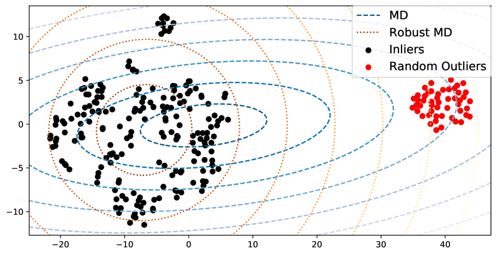
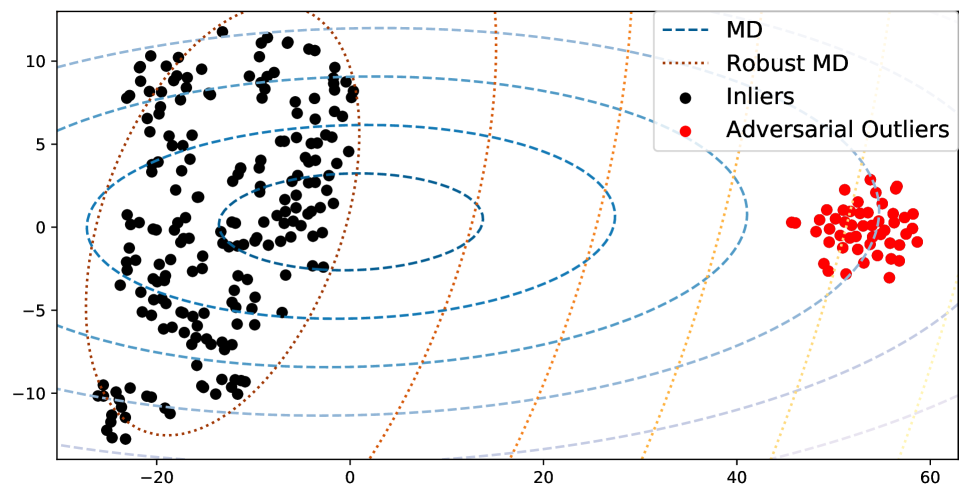
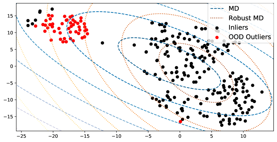
A Motivating Example. We develop techniques to use both MD and Robust MD for anomaly detection, and especially probe the potential of Robust MD-based approach in RL. As a motivating example, Figure 1 shows contours computed by both methods for state feature vectors on the Breakout game from the popular Atari benchmark (Bellemare et al. 2013; Brockman et al. 2016) with different types of outliers. In these results, estimation based on Robust MD is less vulnerable to outlying states (red points), and fits inliers (black points) much better than MD, showing its potential for RL outlier detection.
3 Preliminaries
In this section, we recap the classical Markov Decision Process (MDP) for RL, Proximal Policy Optimization (PPO) algorithm and introduce three kinds of outliers.
3.1 Markov Decision Process (MDP)
In the tabular setting, the interaction of an agent with its environment can be modeled as a Markov Decision Process (MDP), a 5-tuple (). and are the state and action spaces, is the environment transition dynamics, is the reward function and is the discount factor.
3.2 Proximal Policy Optimization (PPO)
The policy gradient algorithm Proximal Policy Optimization (PPO) (Schulman et al. 2017) has achieved state-of-the-art or competitive performance on both Atari games (Bellemare et al. 2013) and MuJoCo robotic tasks (Todorov, Erez, and Tassa 2012). Typical policy gradient algorithms optimize the expected reward function by using the policy gradient theorem (Sutton and Barto 2018). Here is the -parameterized policy function. Trust Region Policy Optimization (TRPO) (Schulman et al. 2015a) and PPO (Schulman et al. 2017) utilize constraints and advantage estimation to perform the update by reformulating the original optimization problem with the surrogate loss as
| (1) | ||||
where is the generalized advantage function (GAE) (Schulman et al. 2015b). PPO introduces clipping in the objective function in order to penalize changes to the policy that make vastly different from 1:
| (2) |
Transitions are sampled by multiple actors in parallel (Henderson et al. 2018). We use PPO as the algorithm testbed to investigate the efficacy of our anomaly detection framework. However, our detection methods are general, and can be easily applied to other typical RL algorithms such as DQN (Mnih et al. 2015; Hessel et al. 2018), A3C (Mnih et al. 2016) and DDPG (Lillicrap et al. 2015).
3.3 Three Types of Outliers
Random Outliers. Random outliers represent state observations with random noise. We simulate such outliers by applying Gaussian noise with mean 0 and different standard deviations to state observations. This type of noise can also simulate measurement errors.
Adversarial Outliers. For adversarial outliers, we construct white-box adversarial perturbations (Goodfellow, Shlens, and Szegedy 2014; Szegedy et al. 2013; Cao et al. 2020) on state observations for the current policy, following the strategy proposed in (Huang et al. 2017; Pattanaik et al. 2017). Particularly, we denote as the “worst” action, with the lowest probability from the current policy . The optimal adversarial perturbation , constrained in an -ball, can be derived by minimizing the objective function :
where and for . We solve this minimization problem with the Fast Gradient Sign Method (FGSM) (Goodfellow, Shlens, and Szegedy 2014), which is a typical adversarial attack method in deep learning literature. We hereby obtain adversarial outliers that can force the policy to choose .
Out-of-Distribution (OOD) outliers. Due to the discrepancy of data distribution among various environments, we randomly draw states from other environments as the OOD outliers for the current environment. In our experiments, we choose images from other Atari games as OOD outliers.
4 Anomaly Detection in RL Evaluation
In this section, we design our (robust) MD-based detection strategies for the first scenario, the evaluation phase of RL algorithms. In this scenario, a fixed RL policy is given. We estimate a detector for this policy in two cases: first, with clean dataset, and second with dataset containing a fraction of contaminated states. This detector along with the RL policy is then applied in the (noisy) real world.
4.1 The Gaussian Assumption
In the evaluation phase, the given parameterized policy can be viewed as a discriminative softmax classifier , where and are the weight and bias of the policy classifier for action class , and is the output of the penultimate layer of the policy network , serving as the state feature vector. Here we denote as the size of the action space and as the mean vector of falling into the action class . Following the conclusion from (Lee et al. 2018), if we assume that the class-conditional distribution follows the multivariate Gaussian distribution with a tied covariance in a generative classifier, i.e., , the posterior distribution of is equivalent to the form of a discriminative softmax classifier. This implies that might be fitted in Gaussian distribution during training the policy . However, the tied covariance assumption has been challenged by (Kamoi and Kobayashi 2020) through their visualization experiments. We approximate state feature vectors with a class-conditional Gaussian distribution and for each action class, rather than use a single “tied” covariance across all action classes. The effectiveness of our Gaussian parametric method is verified in the experiment section.
4.2 Mahalanobis Distance
The Gaussian assumption allows us to use a Mahalanobis distance-based detection, where the mean vectors and the covariance matrix capture the data distribution of for each action class . We firstly collect state action pairs , separately for each action class , and compute the empirical class mean and covariance of :
| (3) | ||||
Mahalanobis distance is superior to Euclidean distance in many tasks (Lee et al. 2018; Ren et al. 2021; Kamoi and Kobayashi 2020), since it utilizes additional data covariance information to normalize the distance scales.
After the estimation in Eq. 3, we obtain the class-conditional Gaussian distribution to describe the structure of the data within the state representation space for each action class. For each state that the agent observes, we compute its Detection Mahalanobis Distance between and the closest class-conditional Gaussian distribution:
| (4) |
The image classification work in (Lee et al. 2018) defined a Mahalanobis confidence score to construct a binary (logistic) classifier. This approach heavily relied on having a validation dataset available. In stark contrast, we utilize as the detection metric under the statistical hypothesis test framework. Proposition 1 shows that this Detection Mahalanobis Distance has a Chi-square distribution under the Gaussian assumption.
Proposition 1.
(Relationship between Detection Mahalanobis distance and Chi-Squared distribution) Let be the -dimensional state random vector for action class . Under the Gaussian assumption , the Detection Mahalanobis Distance in Eq. 4 is Chi-Square distributed: .
Please refer to Appendix A for the proof. Based on Proposition 1, we can select a critical value in the specified Chi-Squared distribution to separate normal states from outliers. Given a new state observation and a confidence level , if , then is detected as an outlier. Experiments in Section 6 provide detection results over a range of confidence levels on the Chi-Squared distribution.
4.3 Robust Mahalanobis Distance
The estimation of and in Eq. 3 is based on Maximum Likelihood Estimate (MLE), which is sensitive to the presence of outliers in the data set (Rousseeuw and Van Zomeren 1990; Cabana, Lillo, and Laniado 2021). Thus, MD may not be sufficiently effective in RL anomaly detection. In our outlier scenarios, the agent sequentially gets exposed to outliers in the evaluation phase. The contaminated state observations that agent observes motivate us to use the robust estimator of Robust Mahalanobis Distance (Rousseeuw 1984; Huber 2004) to improve estimation in the presence of extreme state observations. Our detectors are supposed to more accurately reflect the distance between true state observations.
The Minimum Covariance Determinant (MCD) estimator (Rousseeuw 1984; Grübel 1988) is a robust estimator for the mean vector and covariance matrix of a highly contaminated dataset. MCD determines the subset of observations of size that minimizes the determinant of the sample covariance matrix, computed from only these points. The choice of determines the trade-off between the robustness and efficiency of the estimator. Therefore, the robust MCD mean vector and covariance matrix in the action class are computed as
Based on the robust estimation of mean and covariance matrix, we similarly define Detection Robust Mahalanobis Distance as another robust detection metric:
Since the robust Mahalanobis distance can still approximate the true Chi-squared distribution (Hardin and Rocke 2005), we still use the threshold value for detecting outliers as in the Mahalanobis distance case.
4.4 MD-based Detection Algorithm in Evaluation
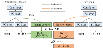
A key issue we need to consider while deploying the detection method is its computational efficiency. We apply Principal Components Analysis (PCA) (Abdi and Williams 2010) on the -dimensional state feature vectors in the penultimate layer of , and conduct MD-based detection in the resulting lower-dimensional representation space. Figure 2 shows a detailed explanation of the outlier detection pipeline in the evaluation phase.
-
•
During the estimation of detectors, when the agent exposes the contaminated state observations, we perform the (robust) estimation on the mean vector and covariance matrix within each action class under the Gaussian assumption.
- •
A detailed practical algorithm is given in Algorithm 1.
5 Anomaly Detection in RL Training
Training robustness is increasingly important in safe RL, as the agent is more likely to encounter state outliers during training. In this section we extend the (robust) MD-based detection approach to our second scenario, the (online) RL training phase. Compared with the RL evaluation phase, the difficulty lies in that the RL policy is changing, thus our detector also changes corresponding to the changing feature vector output by the policy’s penultimate layer. In this scenario, we continuously do both tasks: train the RL agent, and estimate the detector in the noisy online environment. There are multiple options to handle detected outliers during training, such as direct removal or outlier filling. We focus on removal, and evaluate the resulting training curve of cumulative rewards. We enhance this system with Moving Window Estimation and Double Self-supervised Detectors. Both techniques are pivotal for the empirical success of our anomaly detection framework.
Moving Window Estimation. One crucial hurdle in the online setting is that improving the policy leads to changing of the data distribution when the agent interacts with the environment. To use the information from the updated data distribution, we perform a moving window estimation of PCA and MD. In particular, PCA is updated only infrequently (every few hundred iterations). Based on the constantly updated lower-dimensional state feature vectors, and ( and ) are further estimated. This type of infrequent update resembles the use of the target network in DQN (Mnih et al. 2015), which improves the training stability.
Double Self-Supervised Detectors. One detector may fail to recognize all outliers accurately, and also erroneously exclude true informative clean data. Such detection errors can destabilize the RL algorithm and even worsen its final performance. Our current detector is continually estimated based on self-detected inliers. We additionally estimate another detector based on the detected outliers by the current detector. This second self-supervised detector is used to help check if the detection result from the first detector is consistent with the second one. For example, if the first detector identify a state as inlier (or outlier) and the second detector double-check it is not an outlier (or inlier), then this state will be considered as inlier (or outlier). Otherwise if results conflict from the two detectors, the state will be detected randomly.
5.1 MD-based Detection Algorithm in Training
Algorithm 2 shows our MD-based detection procedure for RL training. It incorporates both moving window estimation and double self-supervised techniques. Inliers and outliers in buffers and are used to update our double detectors. Given , the moving window size. state action pairs are used to estimate and ( and ) for each class. Within each moving window update, for each action class , pairs are newly collected while maintaining the previous state action pairs. In a real-time scenario, such as a recommendation system, we would normally first deploy a pre-trained policy as a warm start in the online system to recommend items for each user. Next, the feedback, such as the click-through rate (CTR), will be observed to update the policy in an online manner. Similarly, in our online detection algorithm, a randomly initialized policy is trained without any outliers in the first half of the training phase. This serves as a pre-trained policy with a pre-estimated detector using inliers. Next, our MD-based detection algorithms are used to detect outliers in the following training process, and then we evaluate the training performance of algorithms with detection.
| Games | Outliers | Perturbation | E1 | E2 | TMD | MD | RMD | Games | Outliers | Perturbation | E1 | E2 | TMD | MD | RMD |
| Breakout | Random | std=0.02 | 49.9 | 50.0 | 50.2 | 51.6 | 63.2 | Enduro | Random | std=0.1 | 50.0 | 49.6 | 49.4 | 50.5 | 86.7 |
| std=0.04 | 52.1 | 60.1 | 62.1 | 63.3 | 88.5 | std=0.2 | 50.0 | 49.7 | 51.2 | 65.9 | 95.9 | ||||
| Adversarial | =0.001 | 71.7 | 86.8 | 87.2 | 88.3 | 90.8 | Adversarial | =0.01 | 97.5 | 99.4 | 99.0 | 99.4 | 95.9 | ||
| =0.01 | 80.5 | 94.8 | 95.2 | 95.3 | 92.6 | =0.05 | 99.4 | 99.4 | 99.0 | 99.4 | 95.9 | ||||
| OOD | Asterix | 56.8 | 49.7 | 49.8 | 50.4 | 90.6 | OOD | FishingDerby | 60.6 | 50.1 | 59.4 | 78.4 | 95.9 | ||
| SpaceInvaders | 49.6 | 49.7 | 50.0 | 50.3 | 89.0 | Tutankham | 53.5 | 49.8 | 50.1 | 56.2 | 95.9 | ||||
| Asterix | Random | std=0.15 | 49.5 | 49.6 | 49.5 | 50.3 | 84.9 | FishingDerby | Random | std=0.2 | 50.0 | 49.8 | 49.9 | 50.4 | 90.1 |
| std=0.2 | 50.0 | 50.3 | 50.4 | 58.5 | 94.9 | std=0.3 | 50.0 | 55.0 | 76.6 | 74.3 | 99.2 | ||||
| Adversarial | =0.001 | 80.9 | 83.2 | 84.8 | 88.3 | 93.8 | Adversarial | =0.001 | 56.6 | 97.3 | 98.8 | 99.4 | 99.2 | ||
| =0.01 | 82.9 | 85.4 | 86.7 | 91.2 | 94.3 | =0.01 | 62.4 | 99.3 | 99.2 | 99.8 | 99.3 | ||||
| OOD | Breakout | 49.6 | 49.8 | 49.8 | 50.1 | 95.0 | OOD | Enduro | 50.0 | 49.7 | 49.5 | 50.0 | 94.5 | ||
| SpaceInvaders | 48.9 | 49.1 | 49.1 | 49.4 | 46.4 | Tutankham | 50.2 | 50.1 | 50.0 | 50.4 | 62.0 | ||||
| SpaceInvaders | Random | std=0.02 | 50.1 | 49.9 | 49.9 | 50.9 | 72.9 | Tutankham | Random | std=0.04 | 50.0 | 49.6 | 49.5 | 49.9 | 79.8 |
| std=0.04 | 51.1 | 66.9 | 71.0 | 72.7 | 96.4 | std=0.06 | 50.0 | 49.4 | 49.3 | 49.7 | 93.2 | ||||
| Adversarial | =0.001 | 55.7 | 91.0 | 92.8 | 94.4 | 95.5 | Adversarial | =0.001 | 51.6 | 87.9 | 88.1 | 92.5 | 94.7 | ||
| =0.01 | 61.6 | 96.9 | 97.3 | 97.8 | 97.3 | =0.01 | 51.9 | 97.5 | 97.1 | 98.8 | 94.8 | ||||
| OOD | Breakout | 49.9 | 50.9 | 51.5 | 51.1 | 80.5 | OOD | Enduro | 50.0 | 97.1 | 97.5 | 99.1 | 94.9 | ||
| Asterix | 49.2 | 50.2 | 53.9 | 50.5 | 97.4 | FishingDerby | 50.0 | 62.4 | 70.8 | 75.5 | 94.7 |
6 Experiments
We conduct extensive experiments on six Atari games to verify the outlier detection effectiveness of both our MD and Robust MD detection strategies in both the evaluation and training phases. Six typical Atari games are divided into two different groups: Breakout, Asterix and SpaceInvaders have nearly static backgrounds, while Enduro, FishingDerby and Tutankham have time-changing or dramatically different backgrounds, which are more challenging.
Baseline Methods. (1) Euclidean distance without standardization (E1) assumes that all features are independent under the Gaussian assumption with 1 standard deviation, and thus the Euclidean distance between two state features directly follows a Chi-squared distribution. (2) Euclidean distance with standardization (E2) additionally standardizes each feature based on E1. This can be considered as a simplified version of our MD method with diagonal covariance matrix. (3) MD with tied covariance (TMD) follows the tied covariance assumption in (Lee et al. 2018), where features among all action classes shares a single covariance matrix estimation. (4) MD is our first method with class-conditional Gaussian assumption. (5) Robust MD (RMD) is our proposed robust variant of MD method against contaminated states in the detector estimation.
6.1 Anomaly Detection in RL Evaluation
During the estimation of detectors, we collect pairs in the replay buffer when the agent interacts with the environment, which contains a fraction of one specific type of abnormal states, such as adversarial outliers. Next, based on this contaminated dataset, we use PCA to reduce the state feature vectors into a 50-dimensional space, then apply MD and Robust MD to estimate mean vectors and covariances. Finally, we evaluate the performance of our detection methods on a balanced new state set with outliers. Given a new state , we compute the detection metric and , respectively, and utilize test statistic with significance level for the detection.
Main results. Table 1 suggests the detection accuracy of both MD and robust MD strategies given and 0 contamination ratio in the estimation, across a wide range of outlier types with different perturbation sizes on each game. Full results across various and fractions of contamination are provided in Appendix B. Based on these results, we can conclude that:
-
•
All MD-based methods, i.e., TMD, MD and RMD, outperform Euclidean distance-based ones, including E1 and E2, verifying the usefulness of covariance matrix information in the RL evaluation setting.
-
•
Robust MD significantly outperforms MD and other baselines in most cases, and is comparable to MD in other cases, e.g., when both MD and RMD can achieve high detection accuracy.
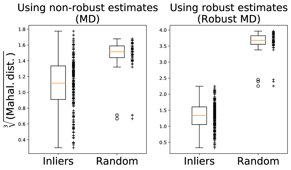
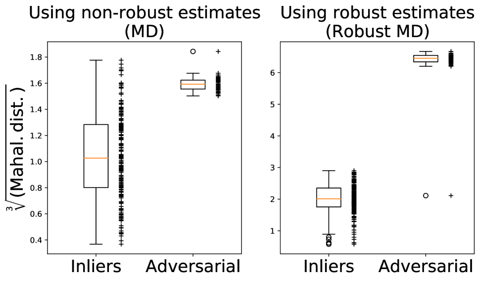
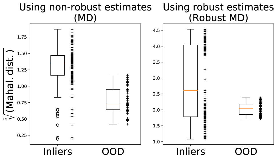
Effectiveness of Robust MD. We have the knowledge that the distribution of outlier states can be more separated from the distribution of inlier states under Robust MD. To demonstrate it, we take the cubic root of the Mahalanobis distances, yielding approximately normal distributions (Wilson and Hilferty 1931). In this experiment, 250 clean states are drawn from the replay buffer, combined with 50 abnormal states from each of three types of outliers. We reduce state feature dimension to 2 via t-SNE, and compute Mahalanobis distances of these two kinds of states to their centrality within each action class under the estimation based on MD or Robust MD, respectively. Figure 3 suggests that Robust MD separates inliers and outliers better than MD on Breakout within a random action class, indicating that robust MD facilitates their identification in the detection. Similar results in other games are given in Appendix C. We also provide sensitivity analysis regarding the number of feature dimension reduced by PCA in Appendix E.
6.2 Anomaly Detection in RL Training
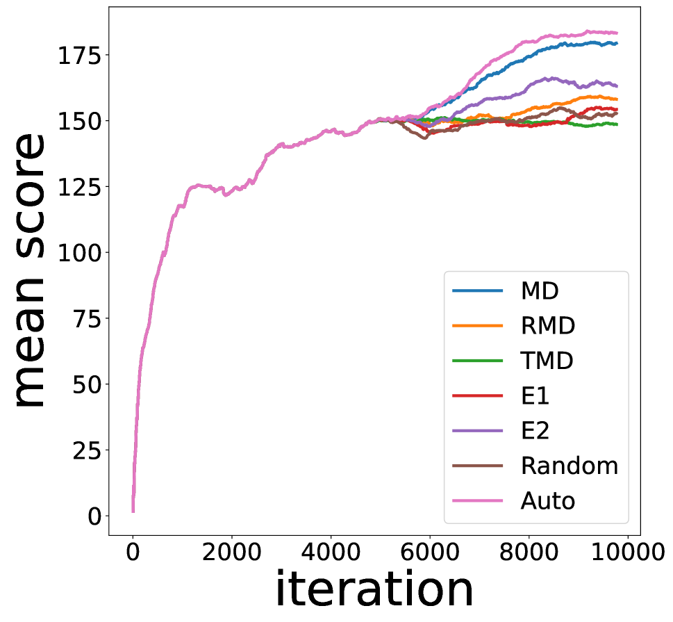


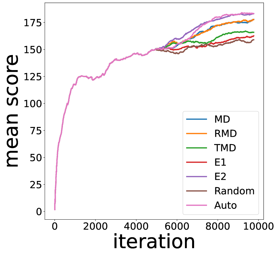

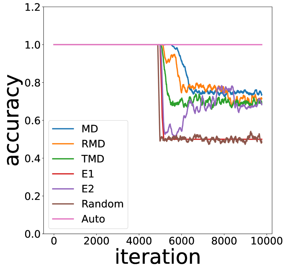
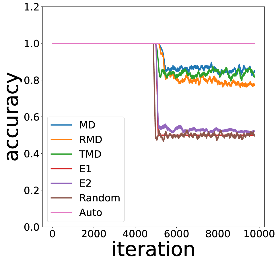


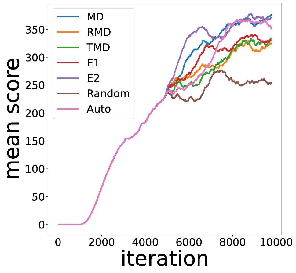
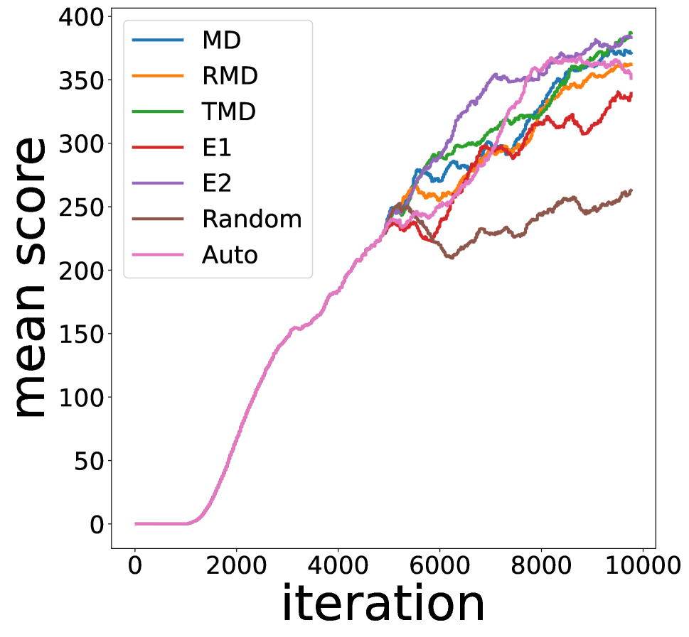
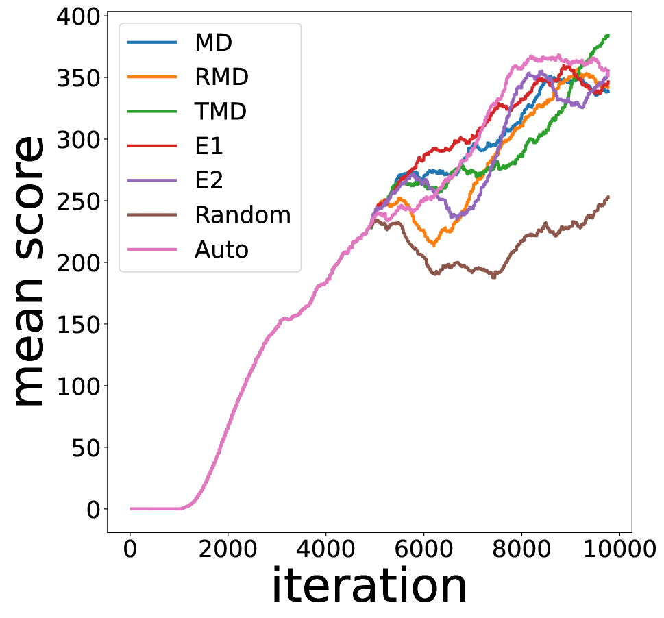
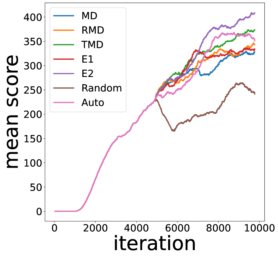
Owing to the parallel training of PPO and the estimation of GAE (Schulman et al. 2015b), we consider discriminating outliers according to a trajectory. We regard a trajectory as outliers if half of its states are detected as outliers. We run eight environments in parallel as in the PPO paper (Schulman et al. 2017) and add state outliers on all state observations in four out of eight environments. For random and adversarial outliers, we directly add noises to original state observations pixel by pixel. For OOD outliers, we choose another different Atari game as the OOD environment and simulate outliers from this different environment. Due to the different action spaces between the original environment and the OOD environment, we draw OOD states from the OOD environment by taking random actions from its own action space. For random and adversarial outliers, actions are taken based on the PPO policy network . For Robust MD method, we use PCA to reduce state feature vectors into a 50-dimensional space due to its expensive computation. For the other methods, we use the original 512-dimensional feature vectors output from the penultimate layer of the policy network . Results are averaged over 3 seeds. Hyper-parameters are given in Table 4 of Appendix F.
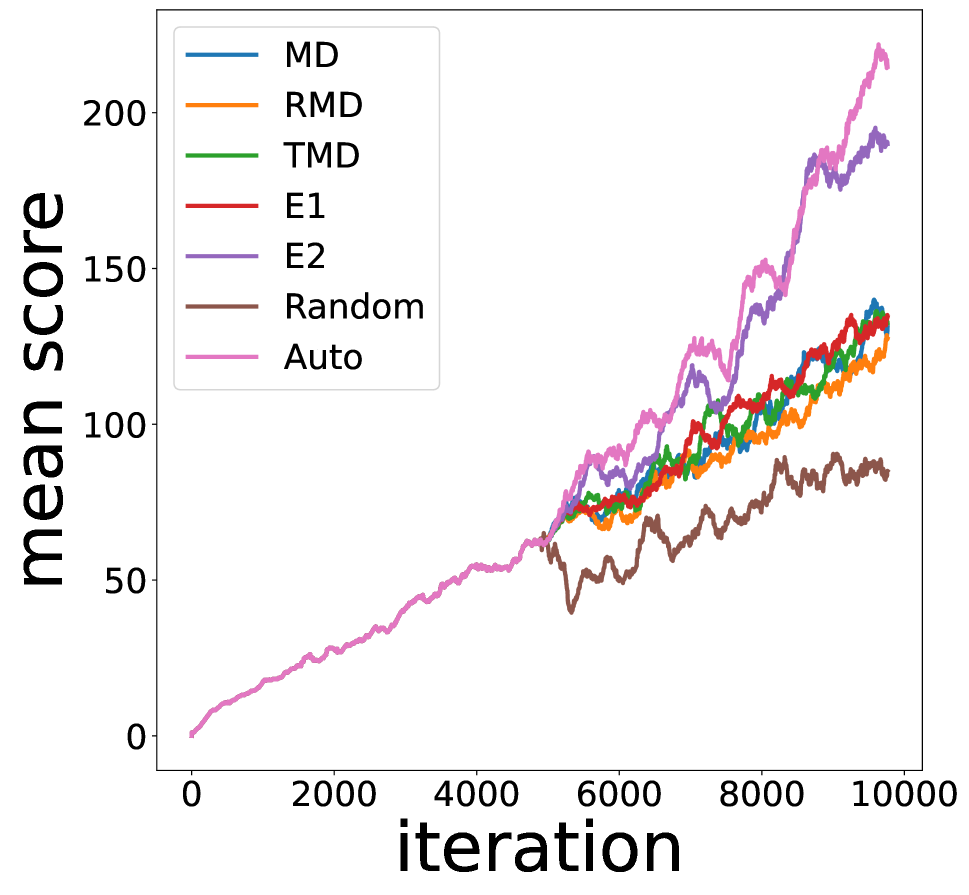
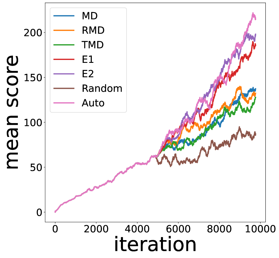
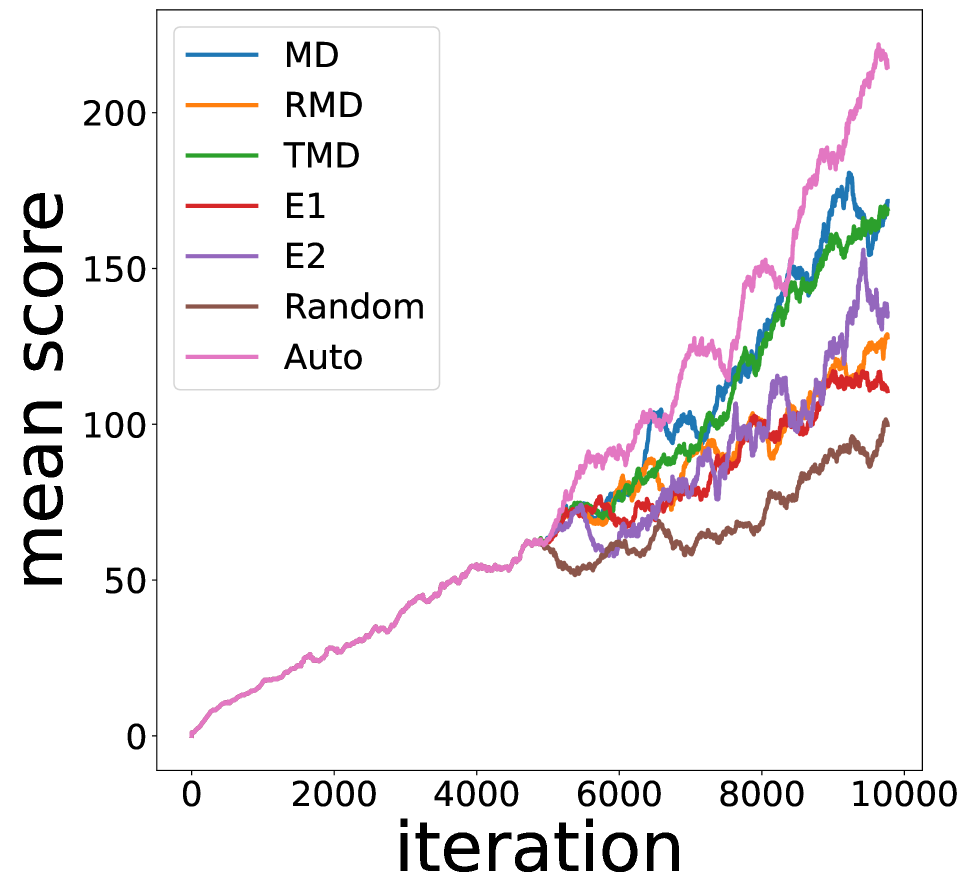
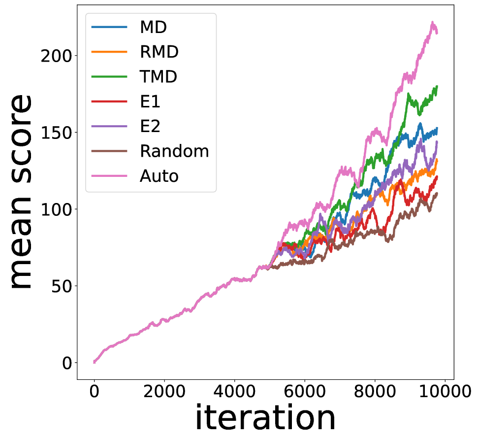
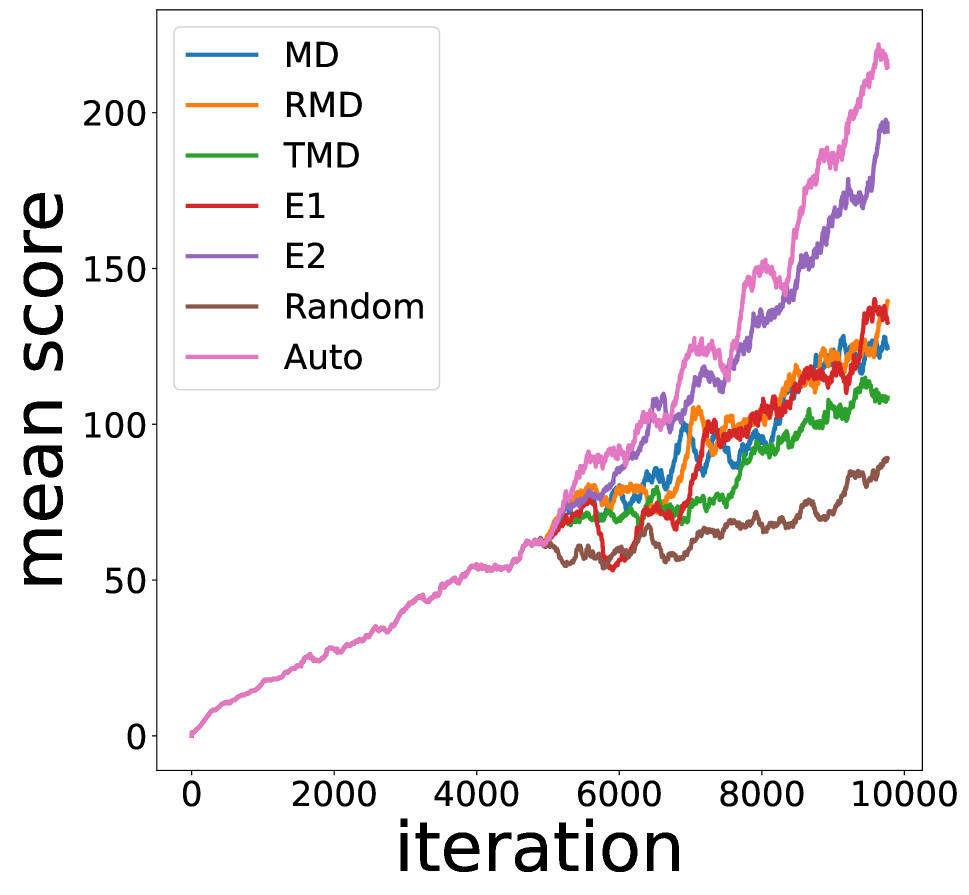
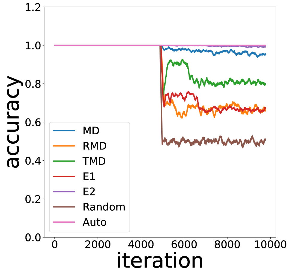
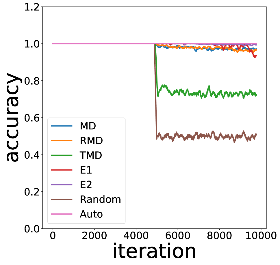
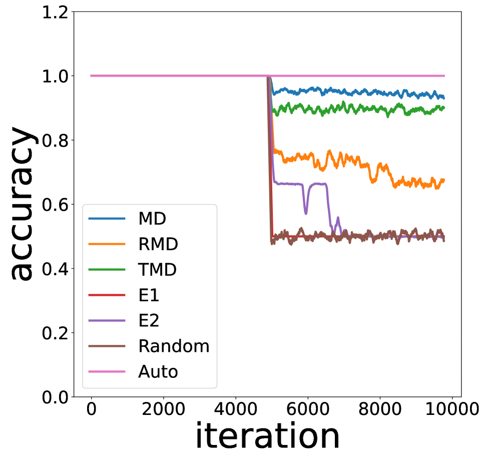
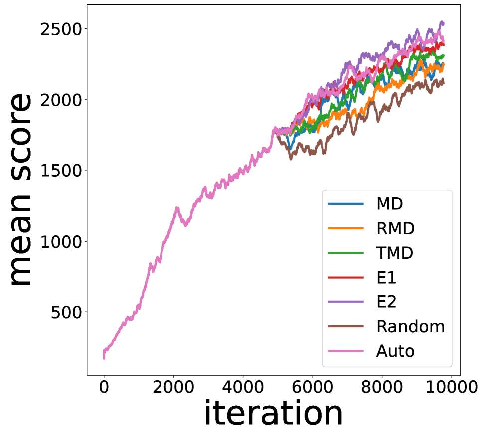
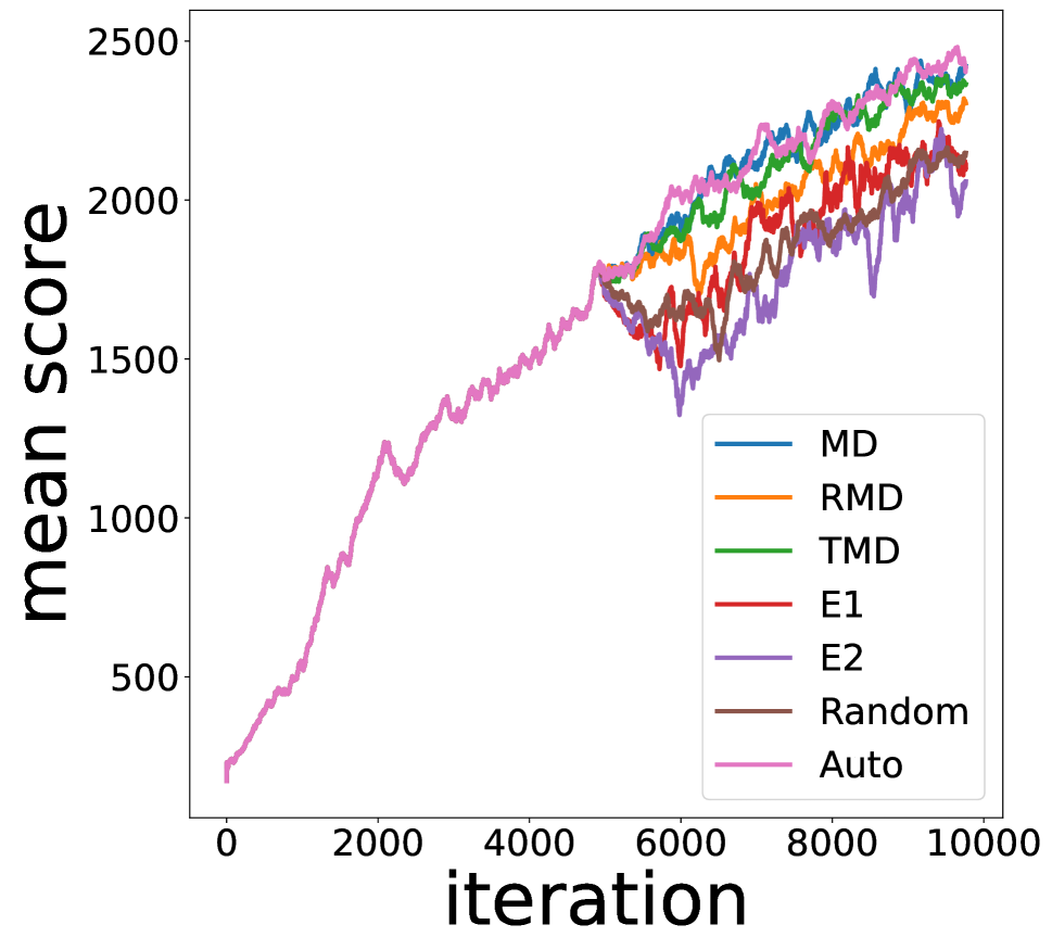
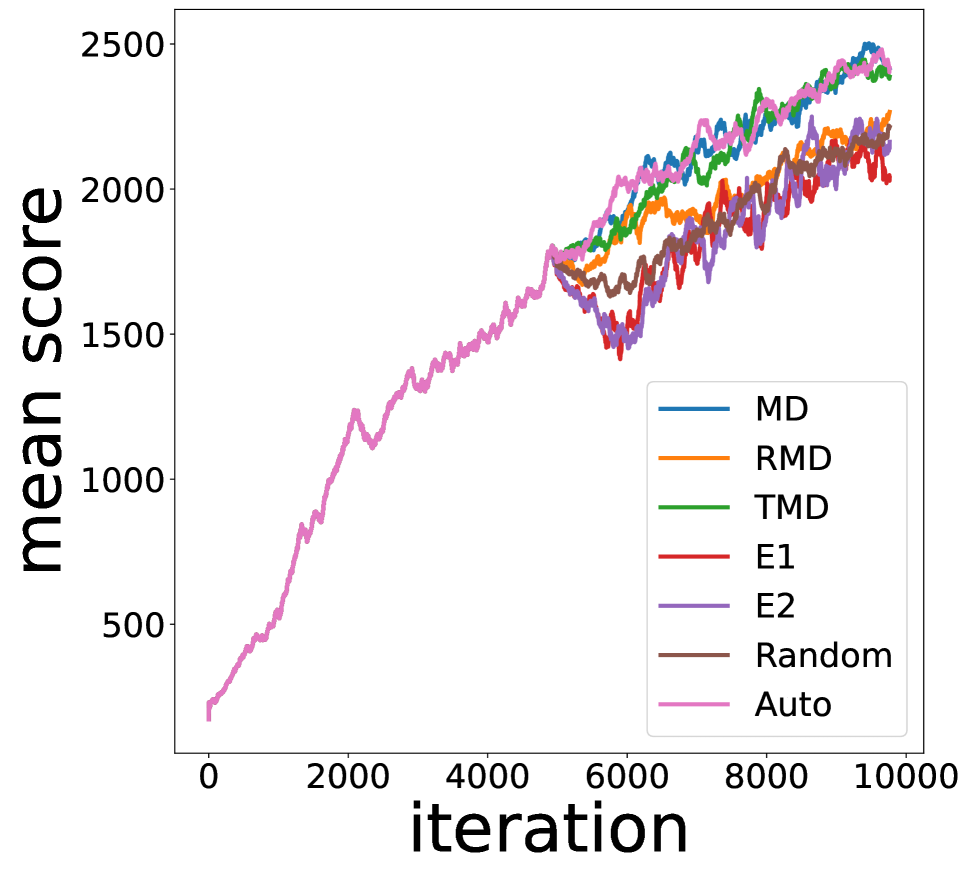
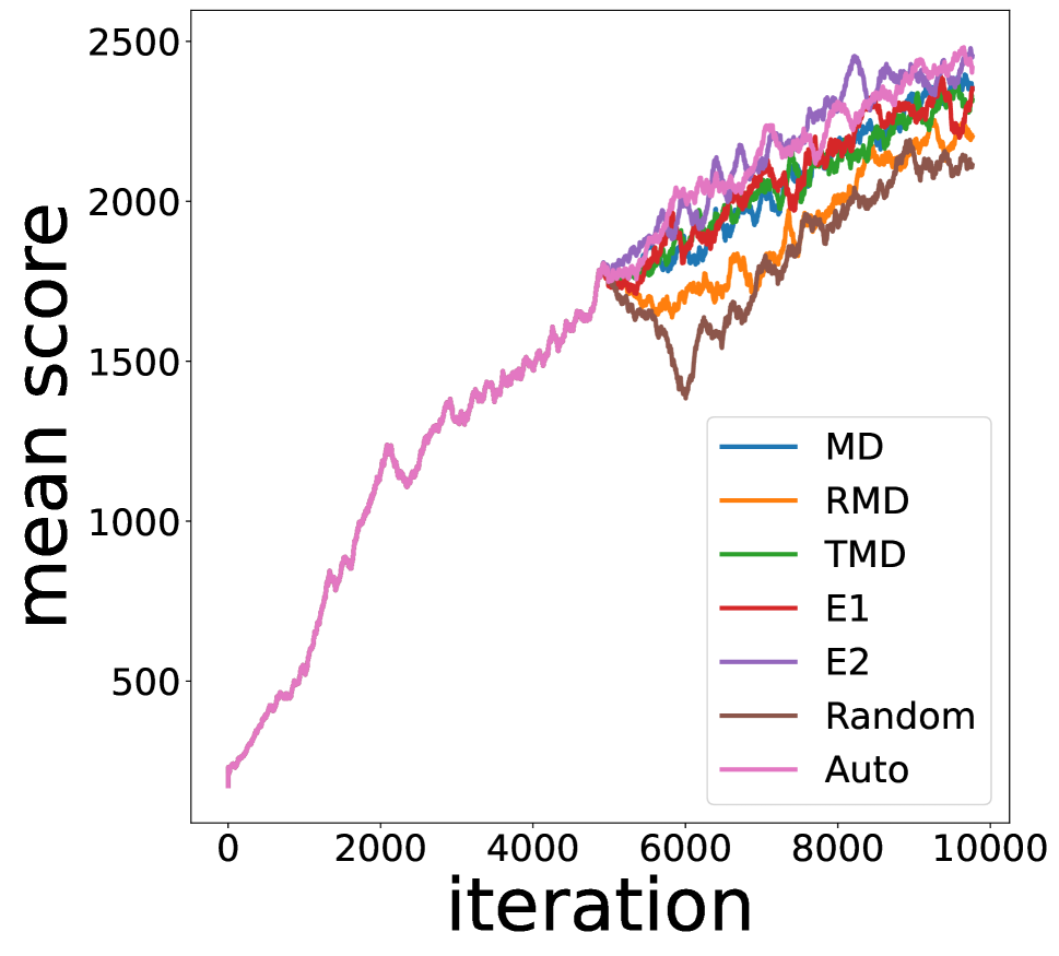
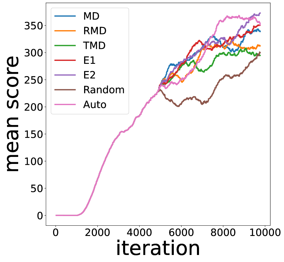
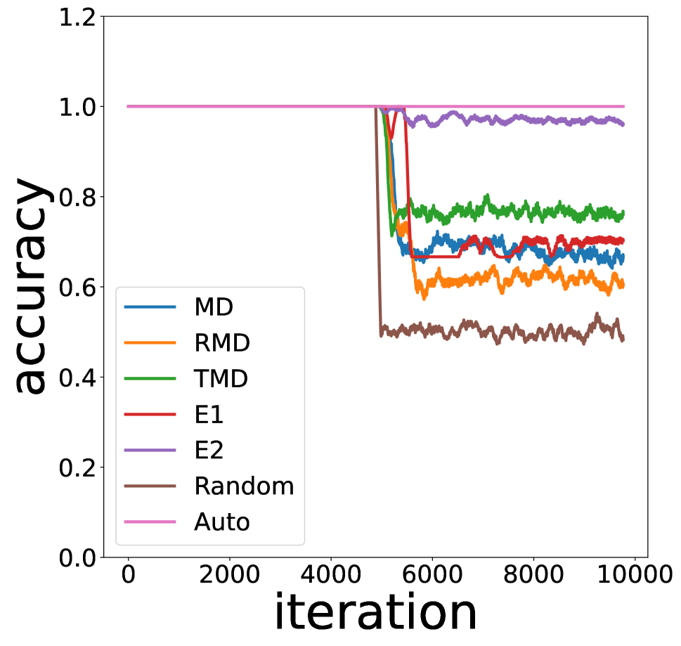
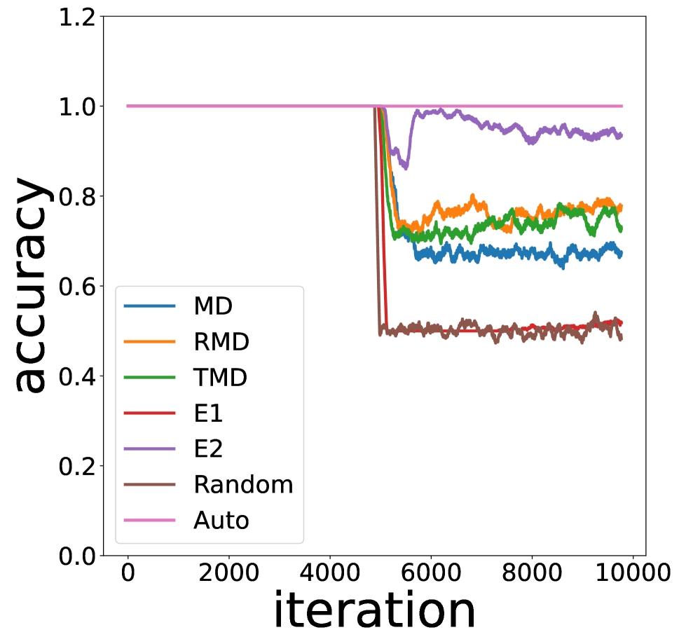
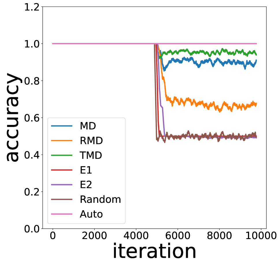
Additional Baseline Methods. We add two other baselines as performance upper bound and lower bound. (1) For an ideal baseline, the method Auto automatically deletes true state outliers, showing the optimal training performance of algorithms without the interruption from outliers. (2) As the other extreme, Random uses a totally random detector.
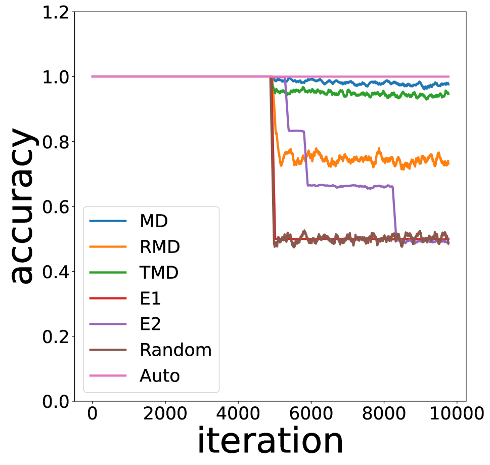
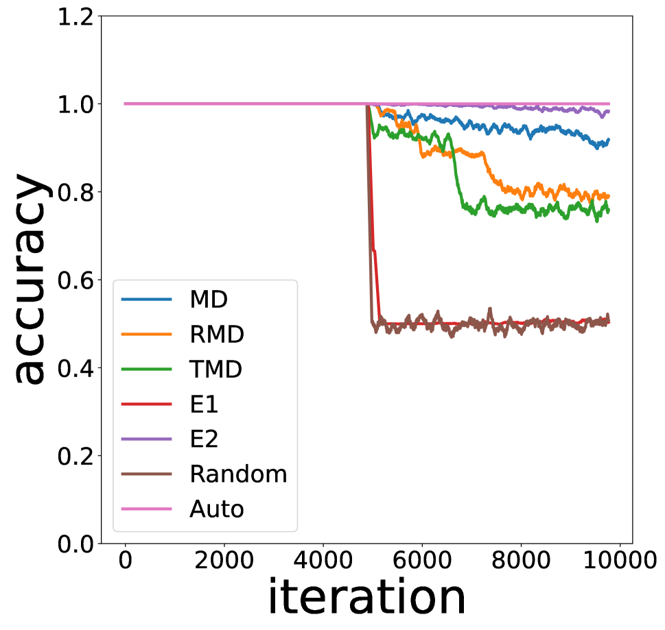
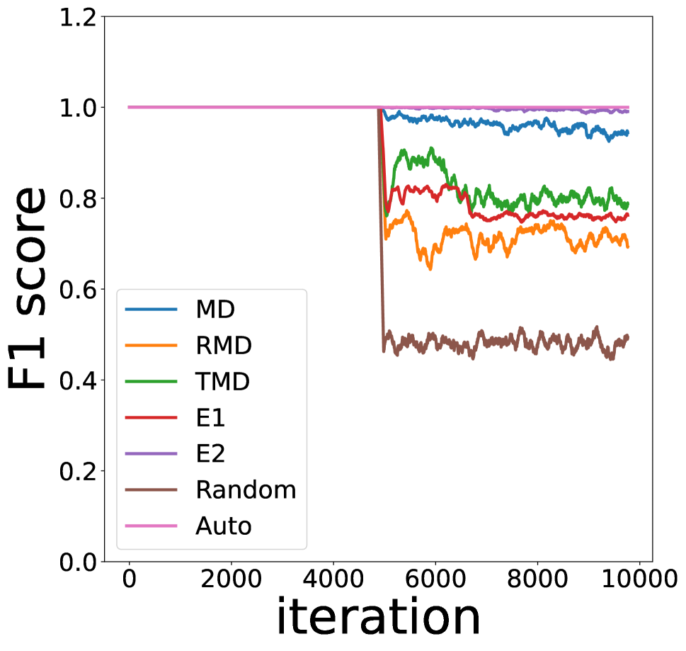
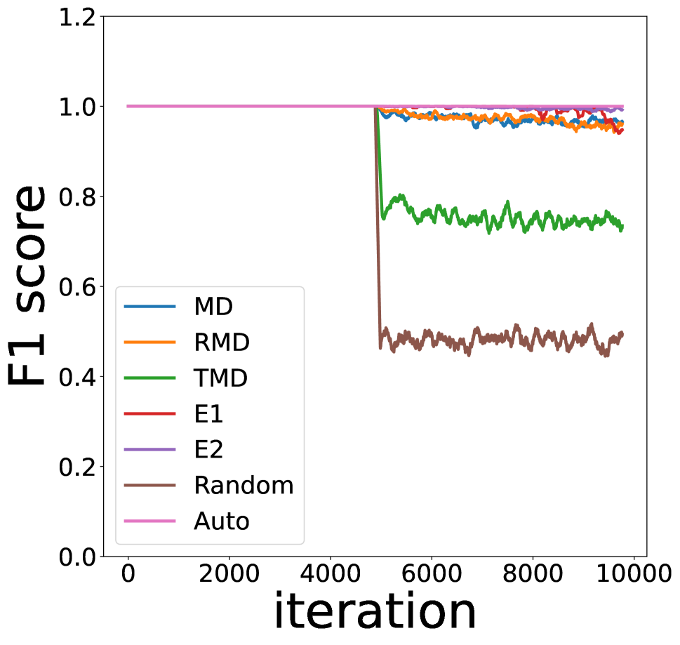
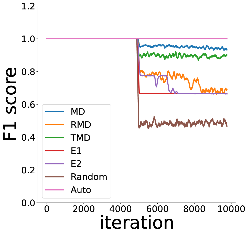
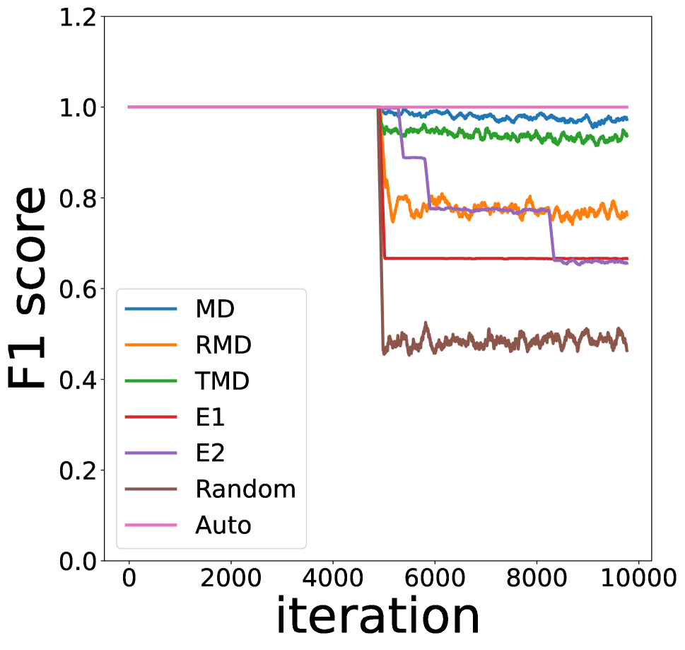
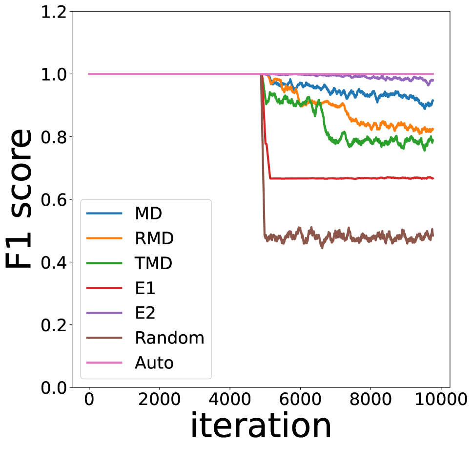
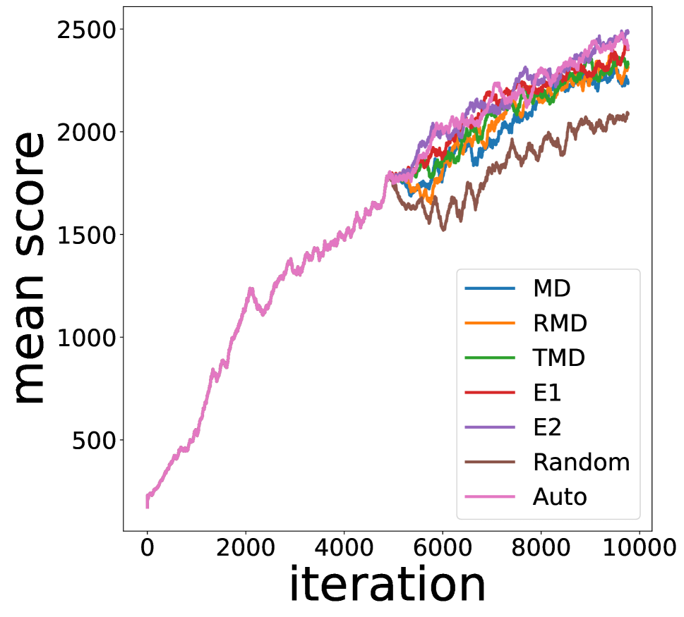
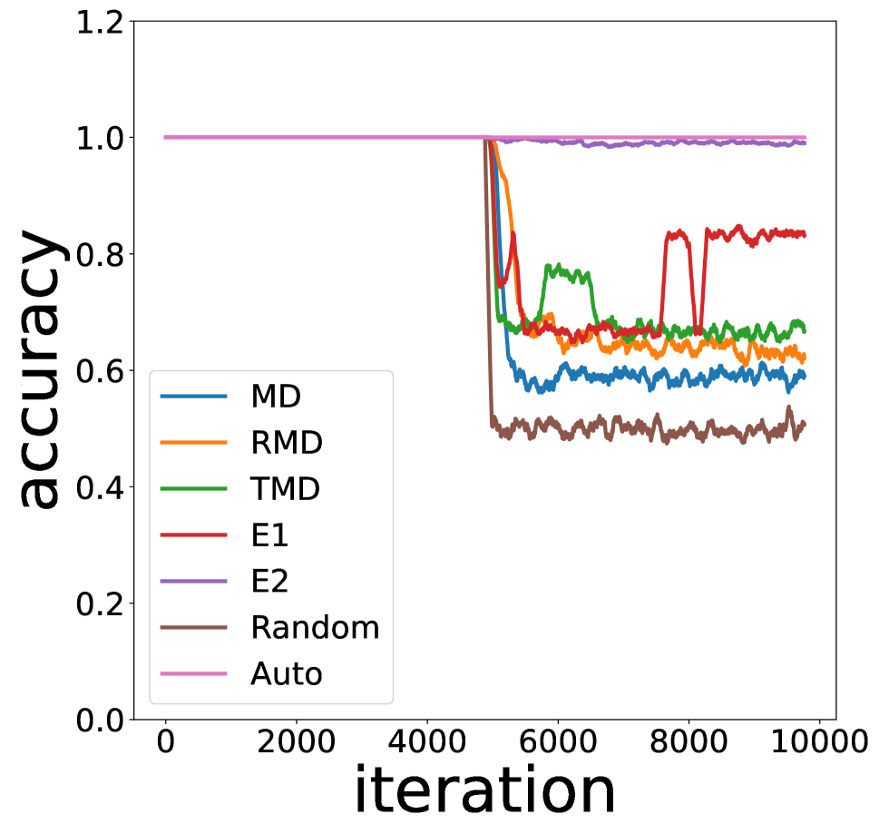
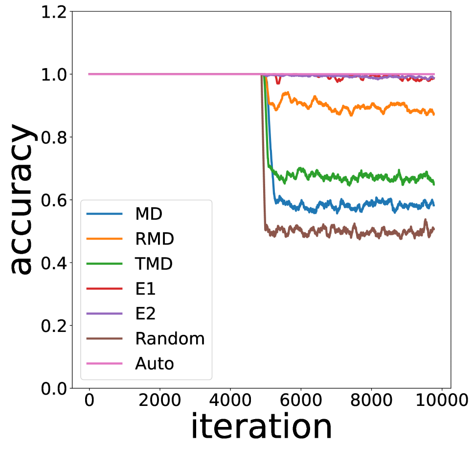
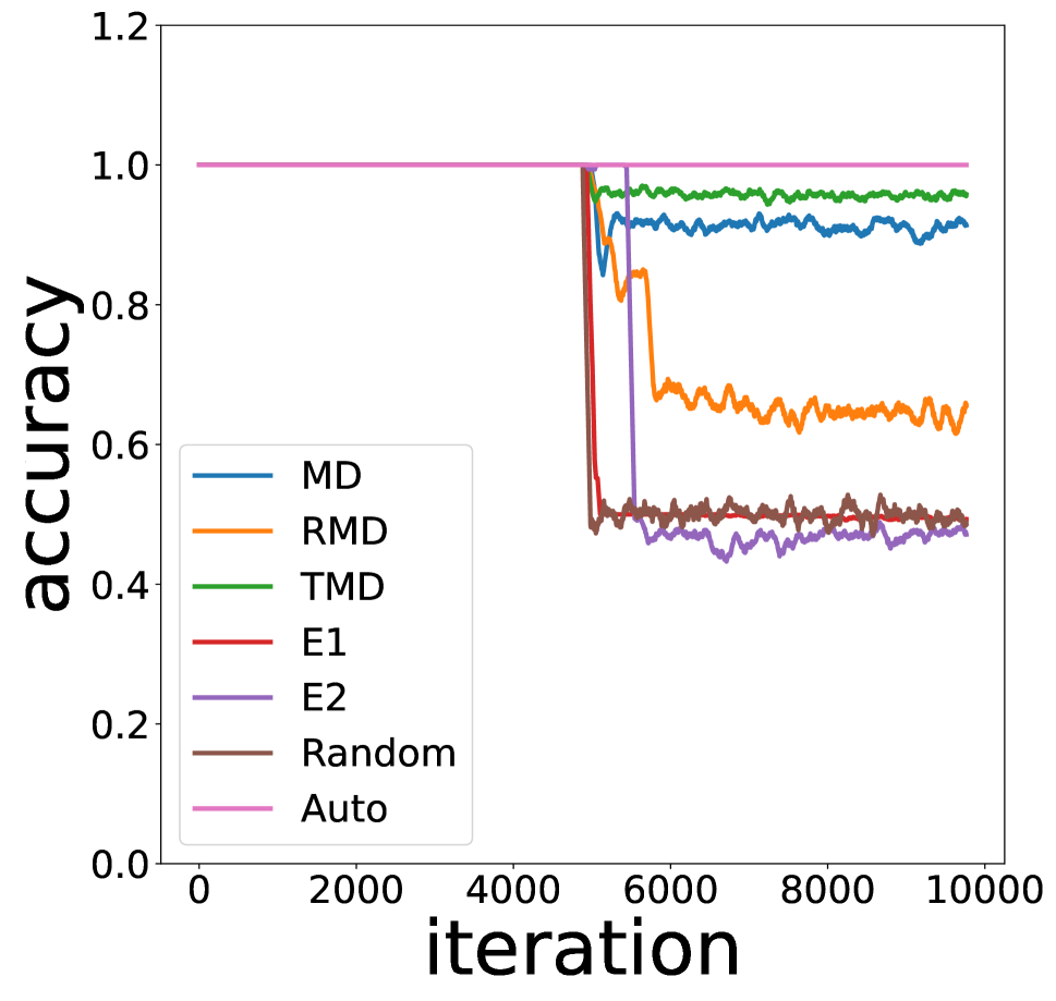
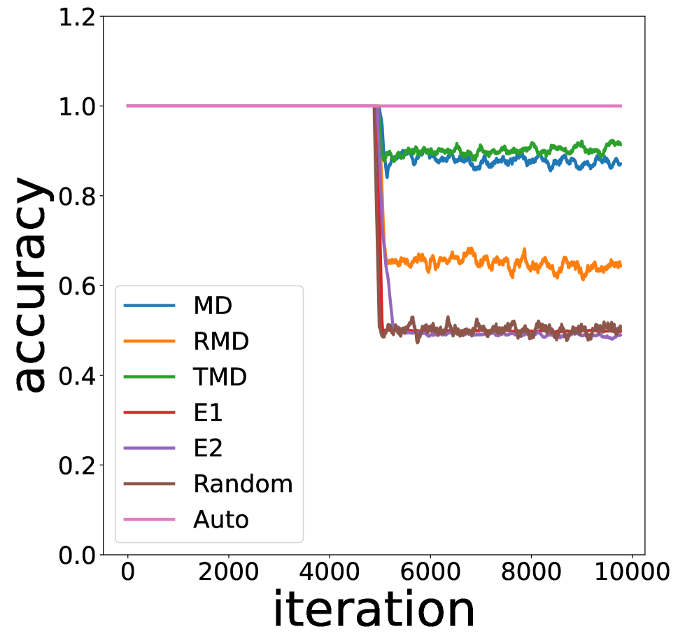
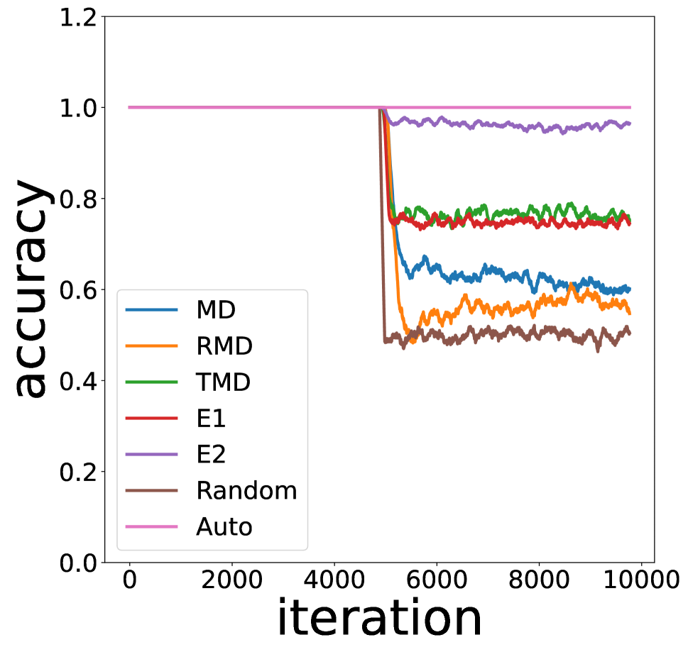
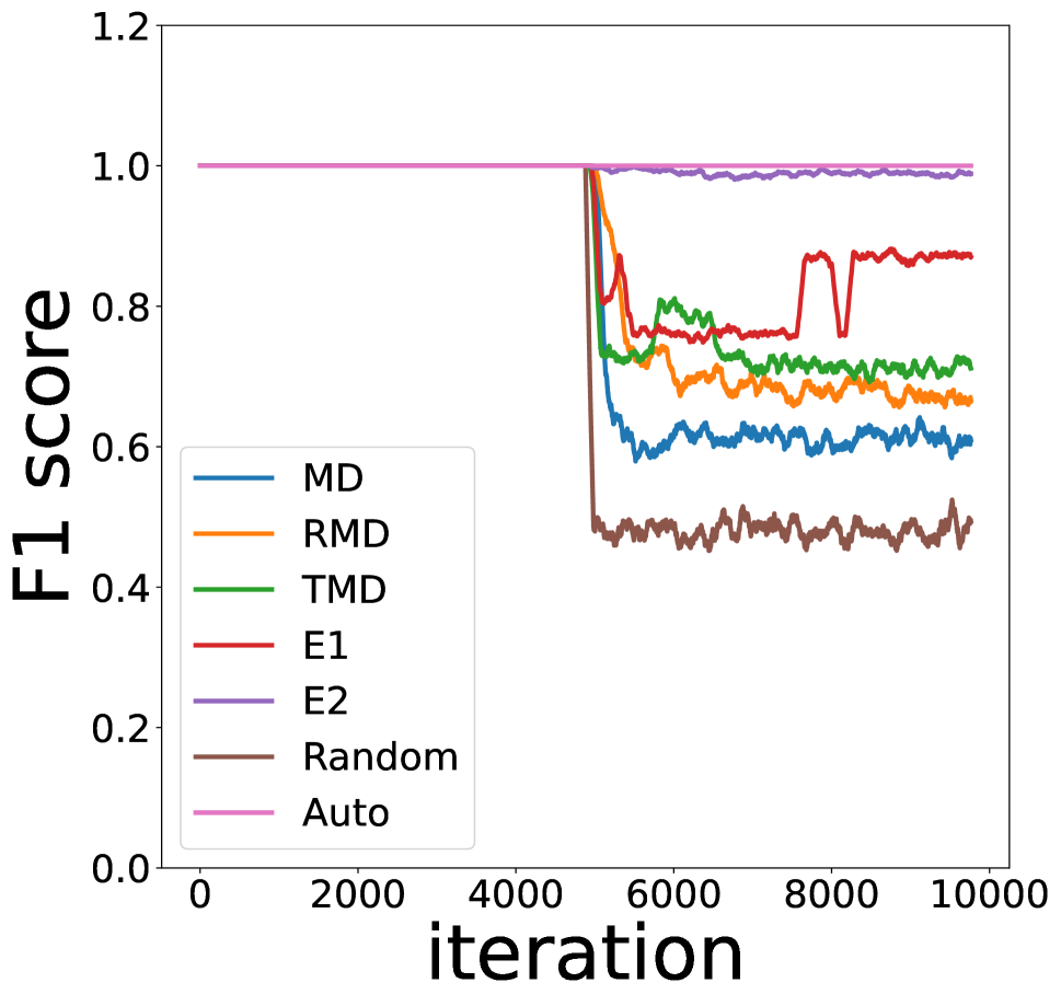
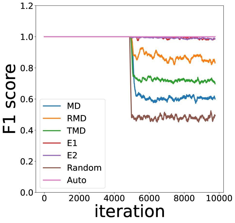
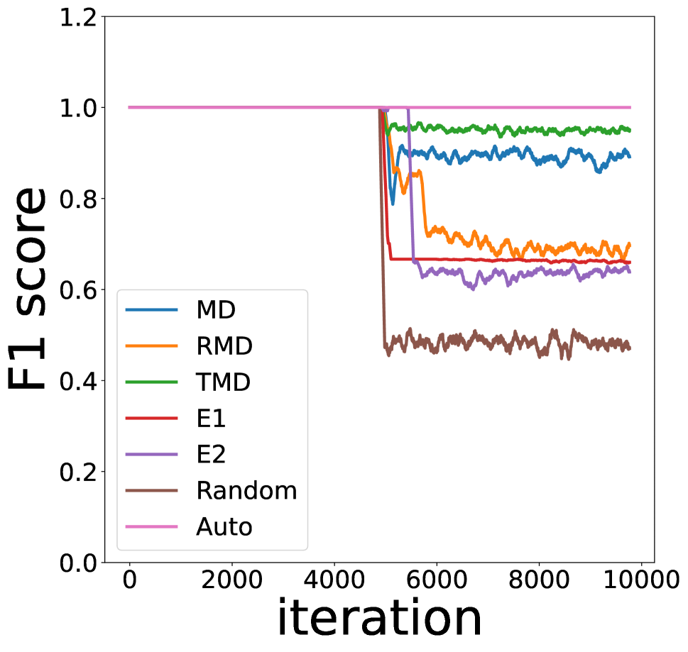
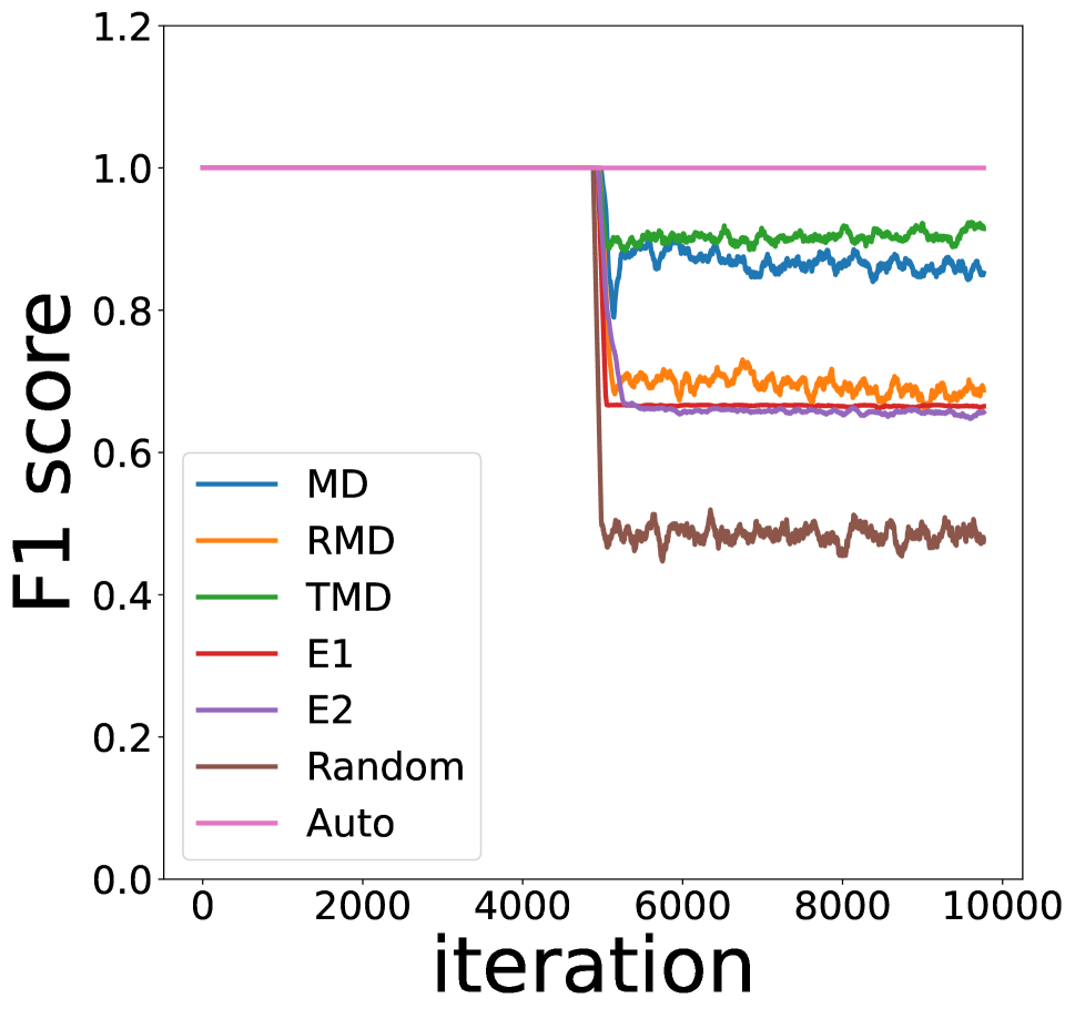
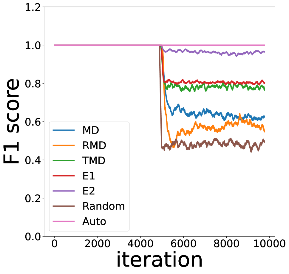
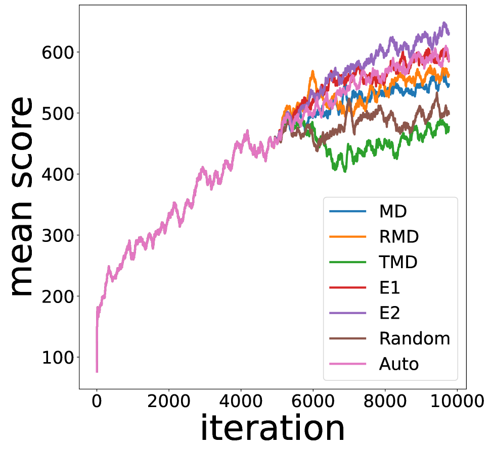
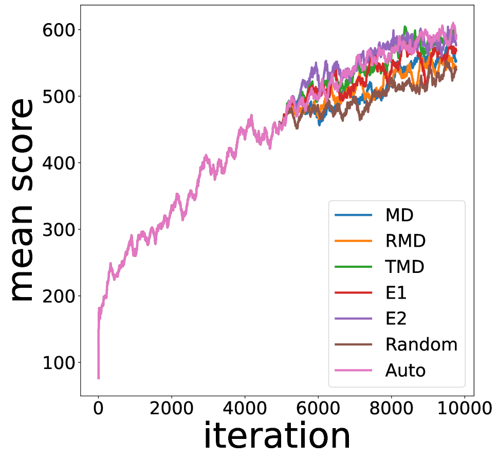
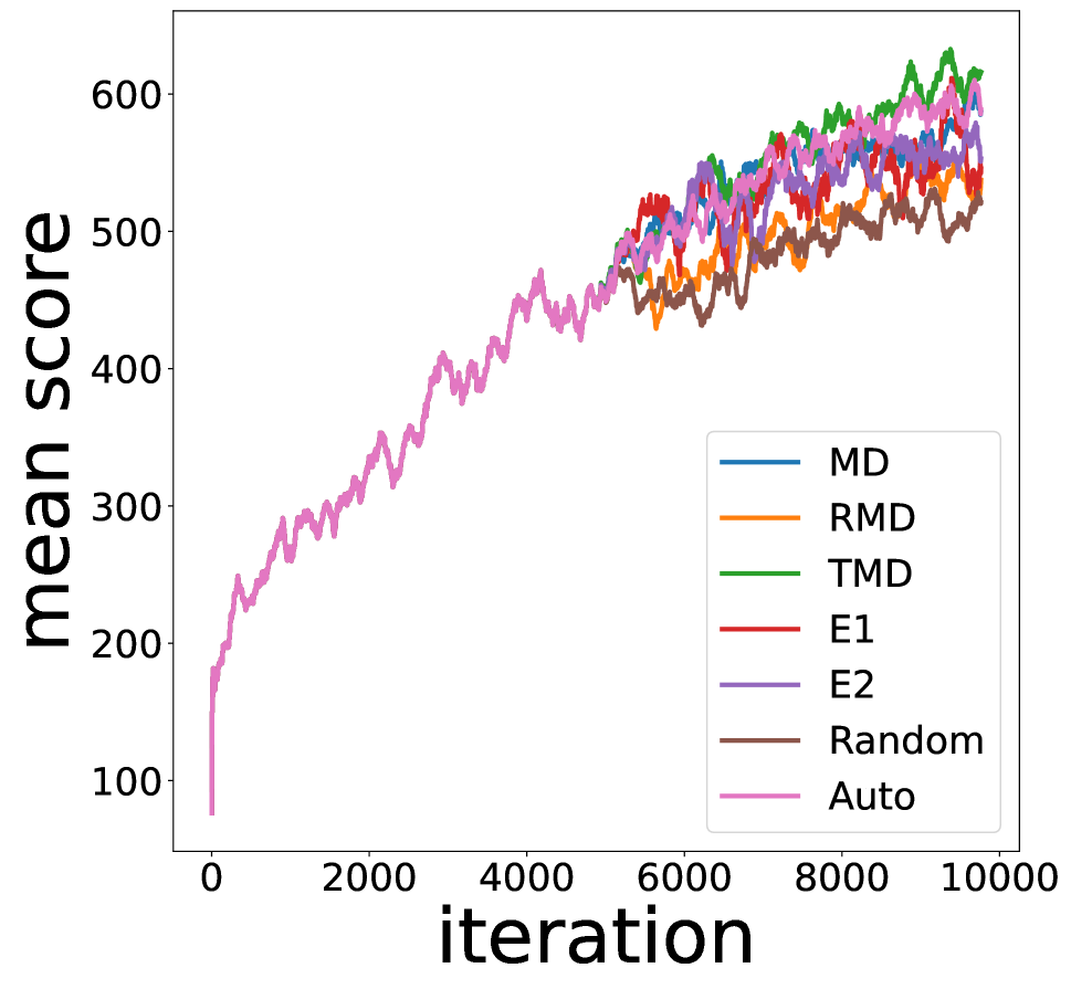
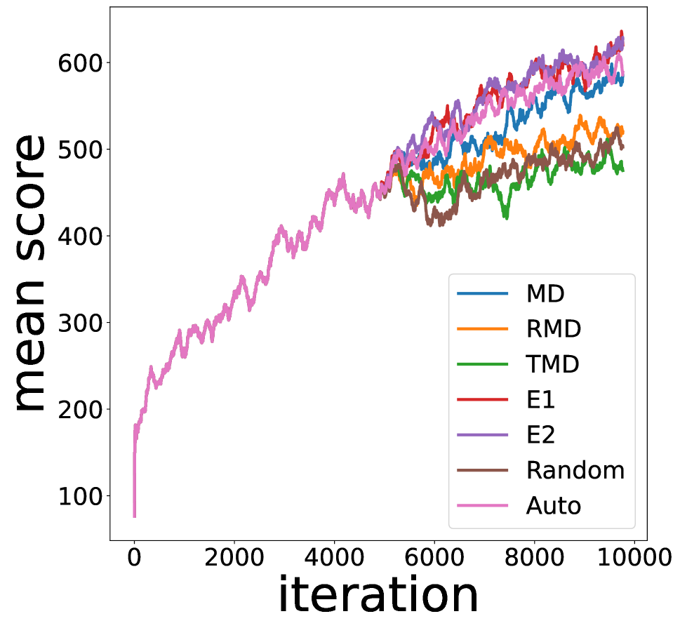
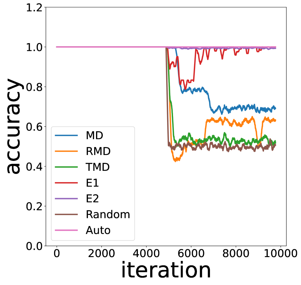
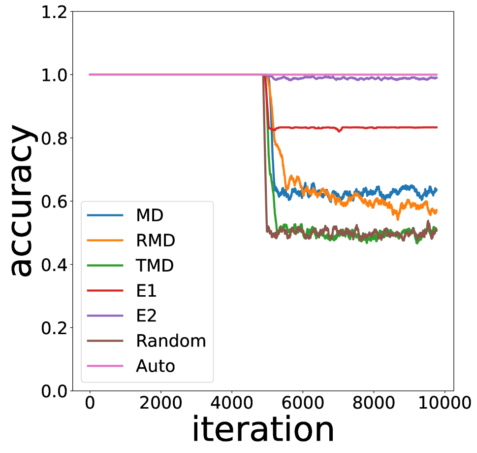
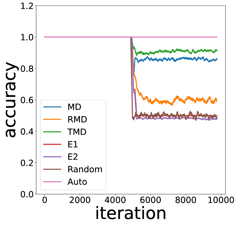
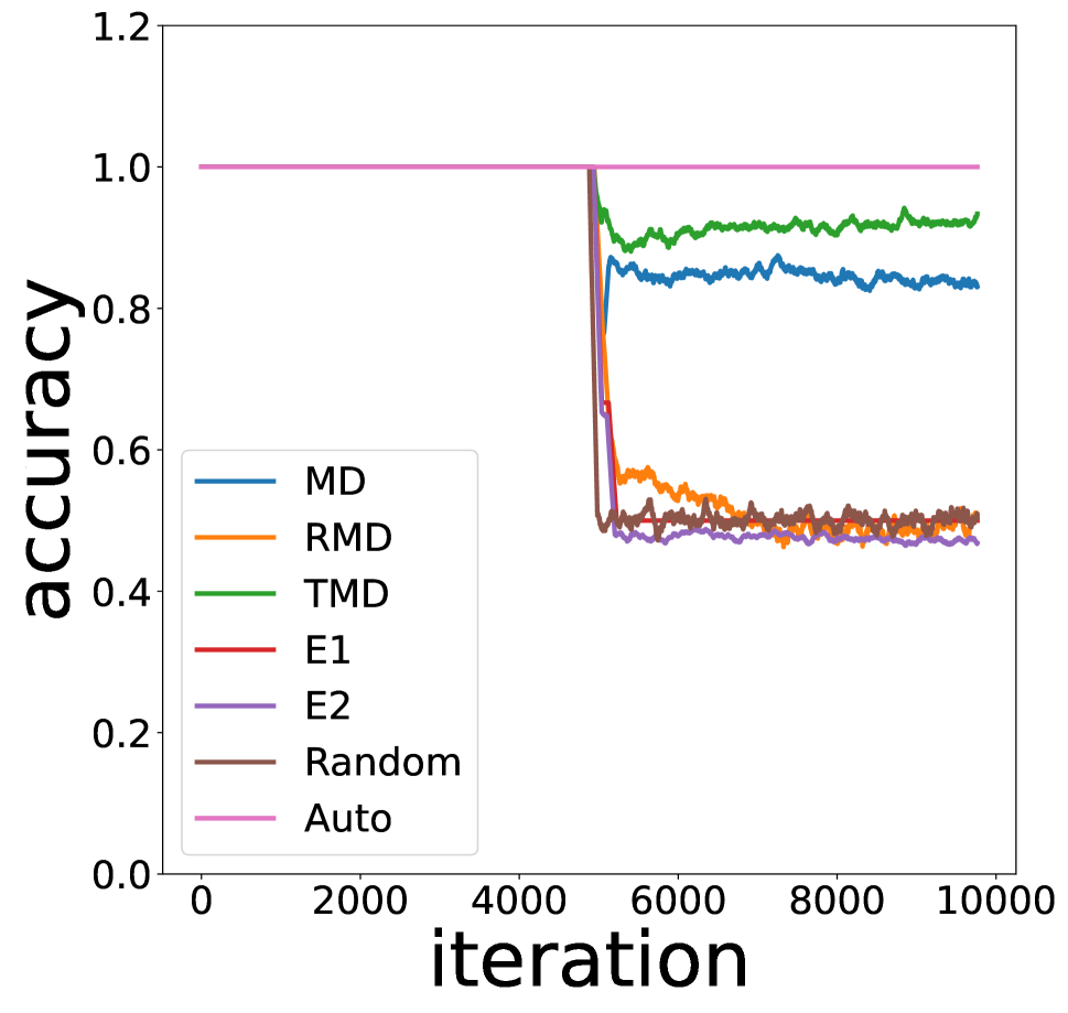
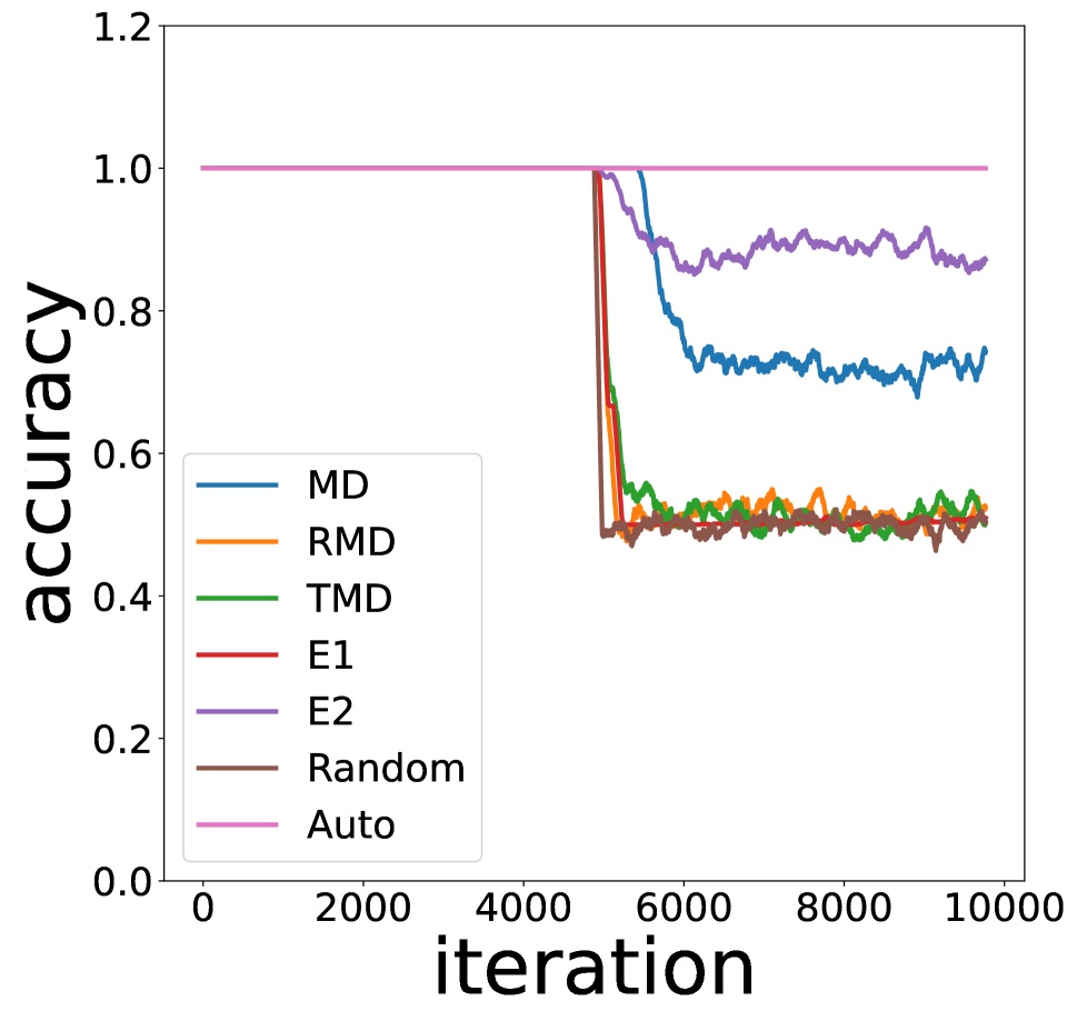
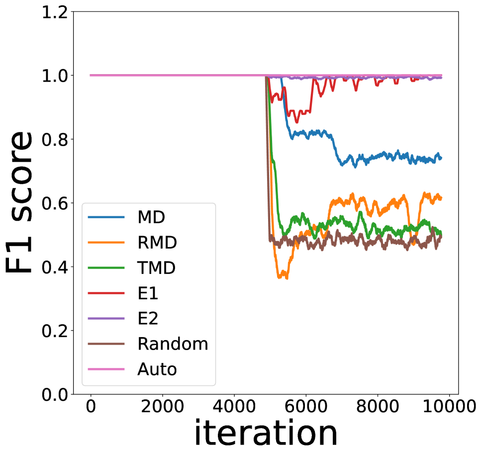
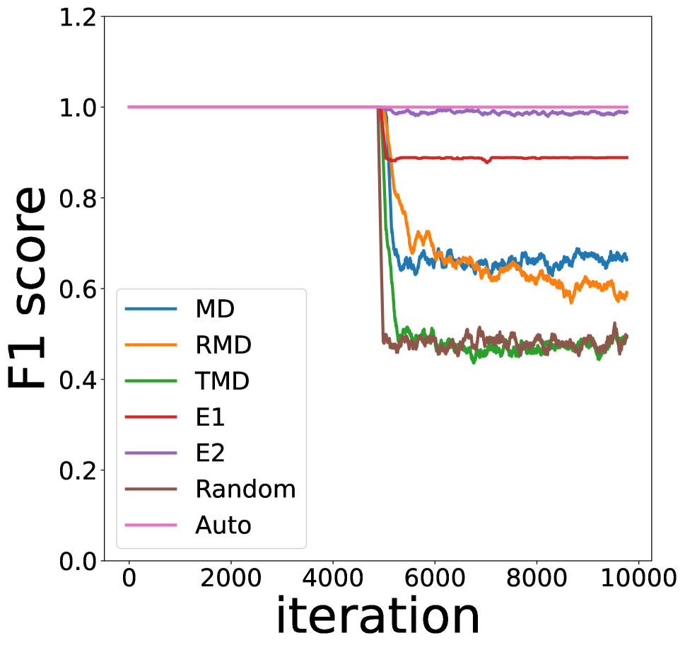
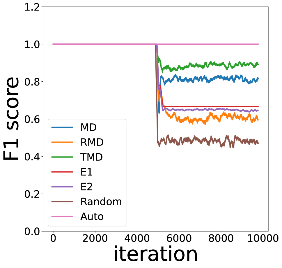
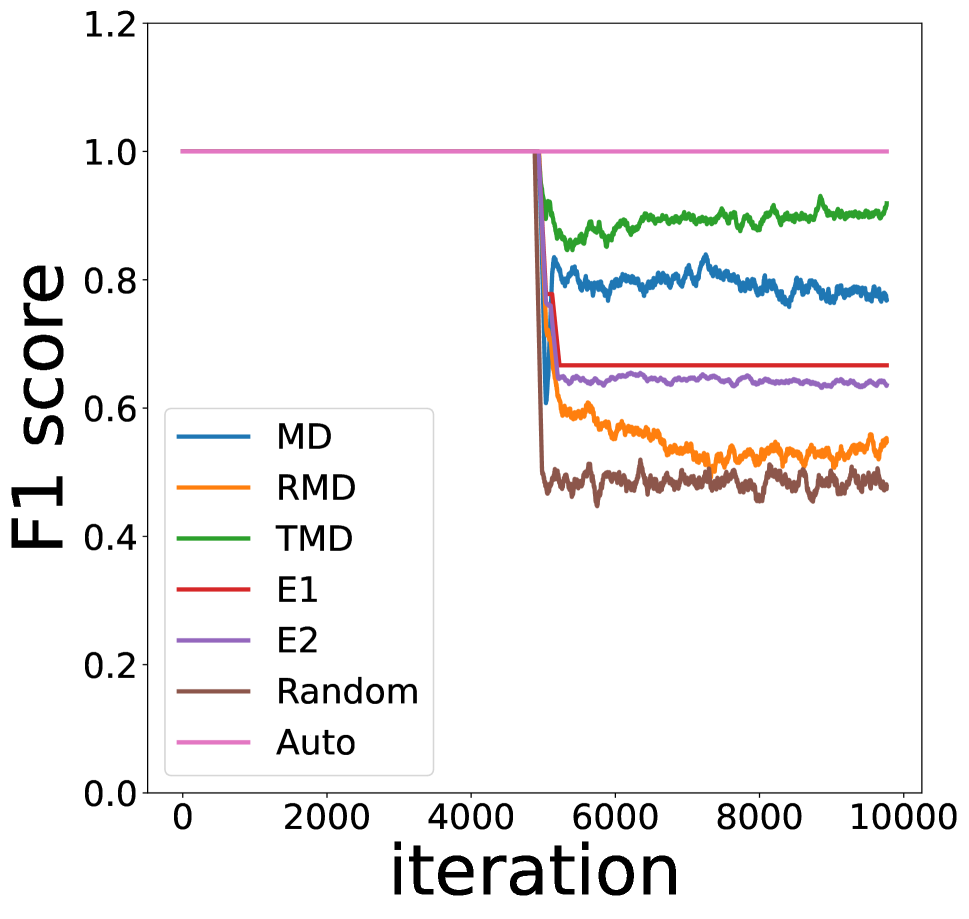
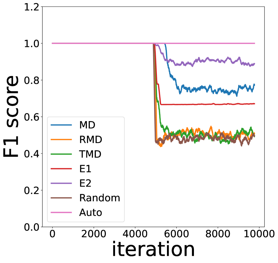
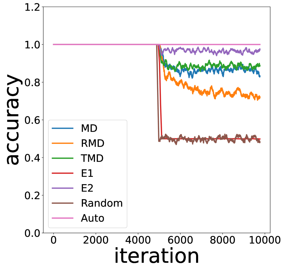
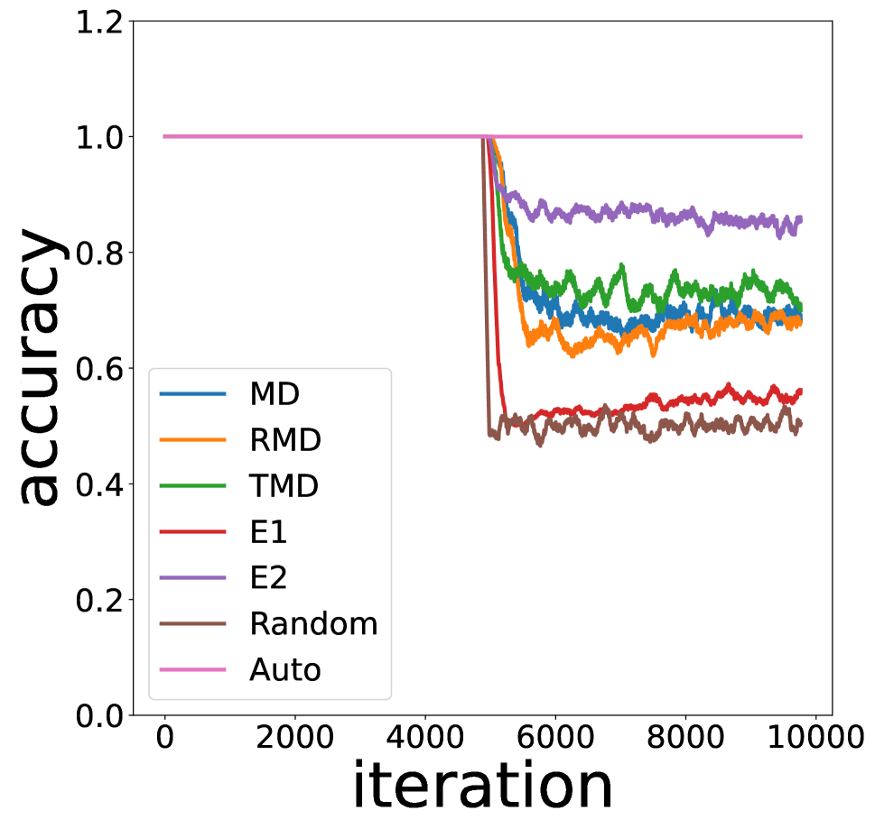
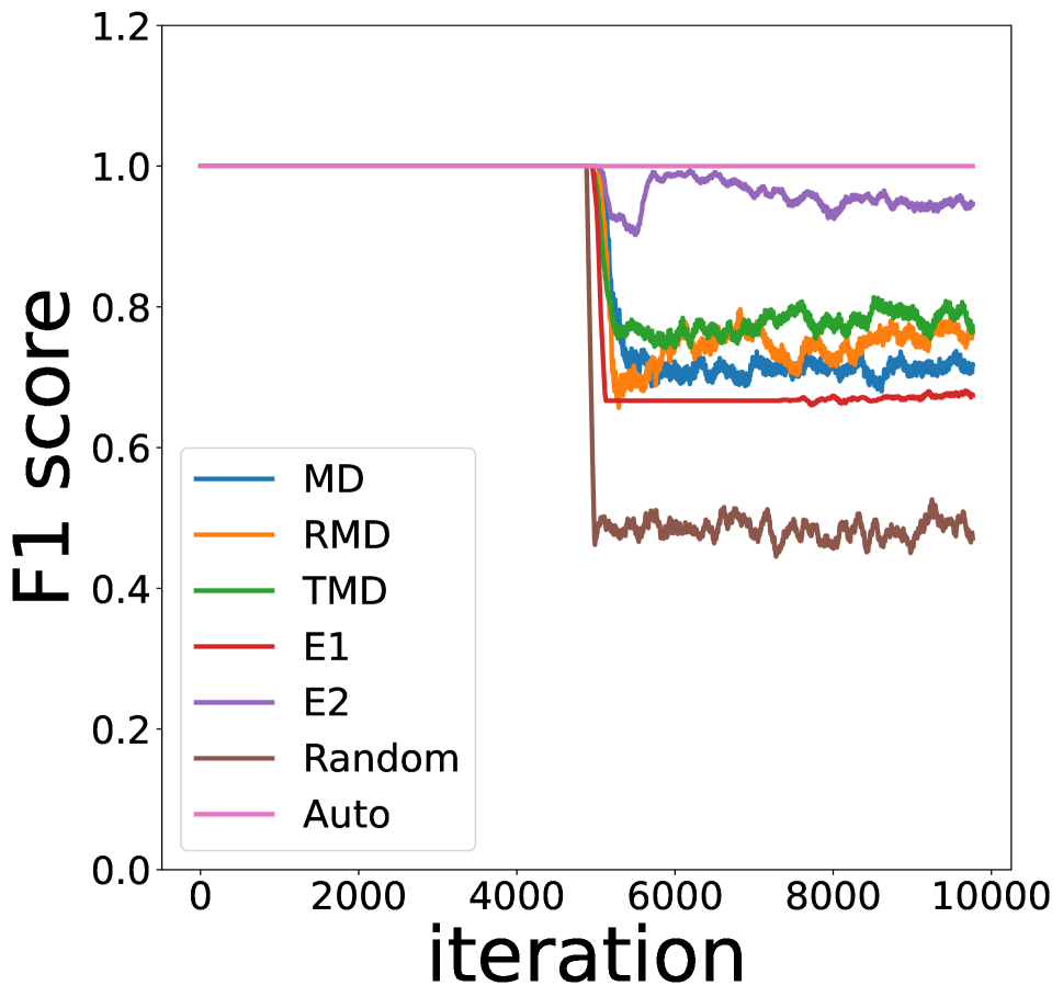
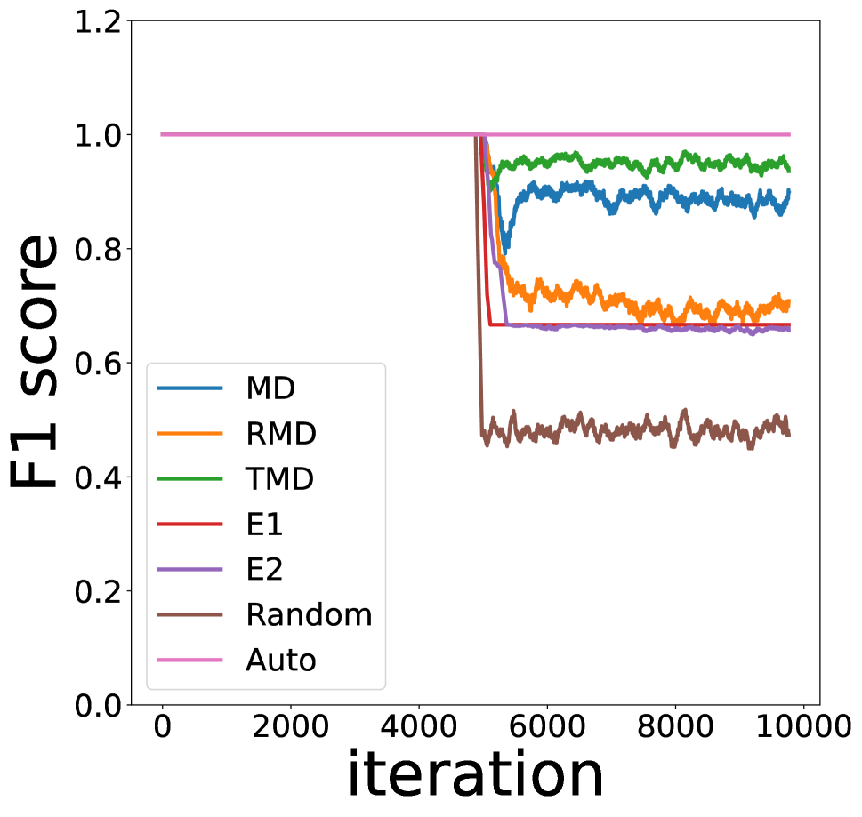
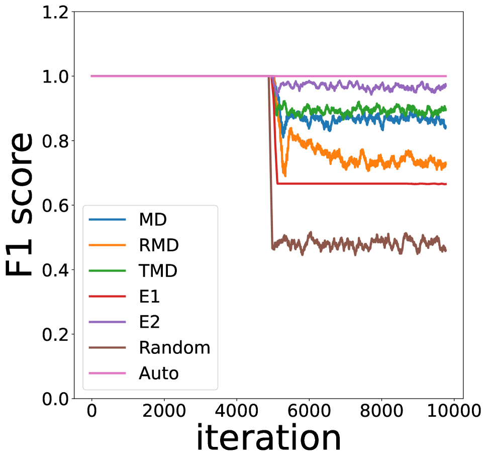
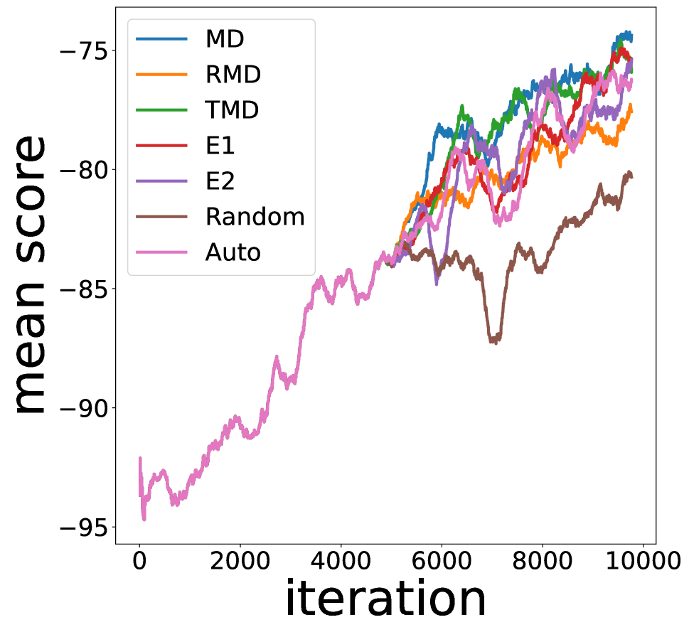
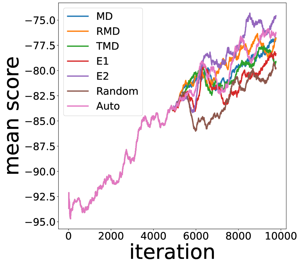
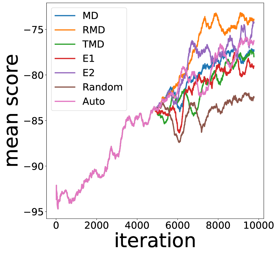
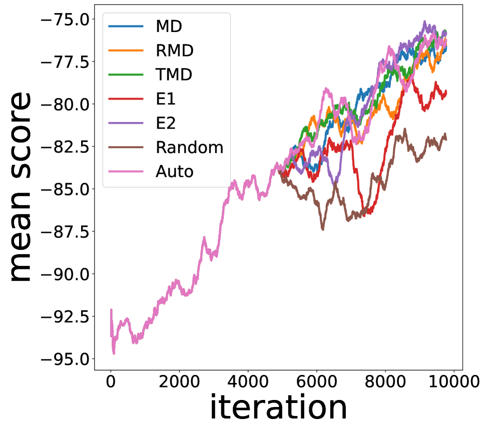
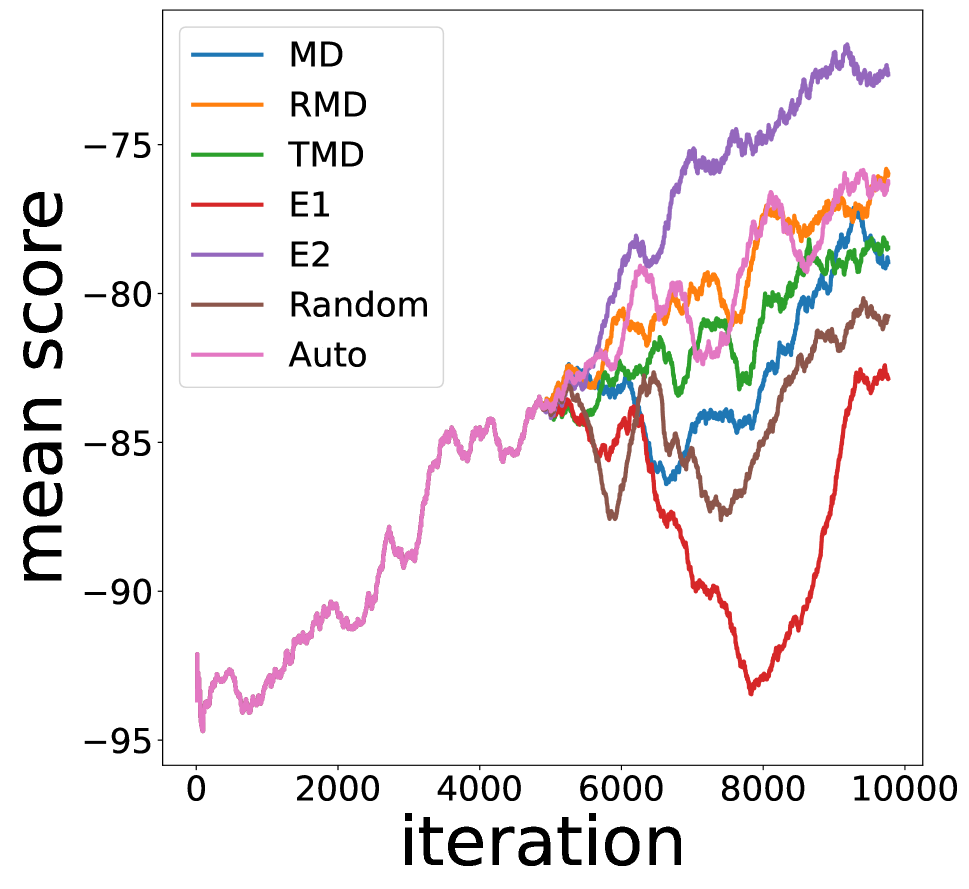
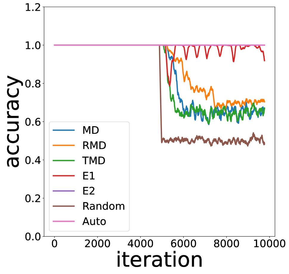
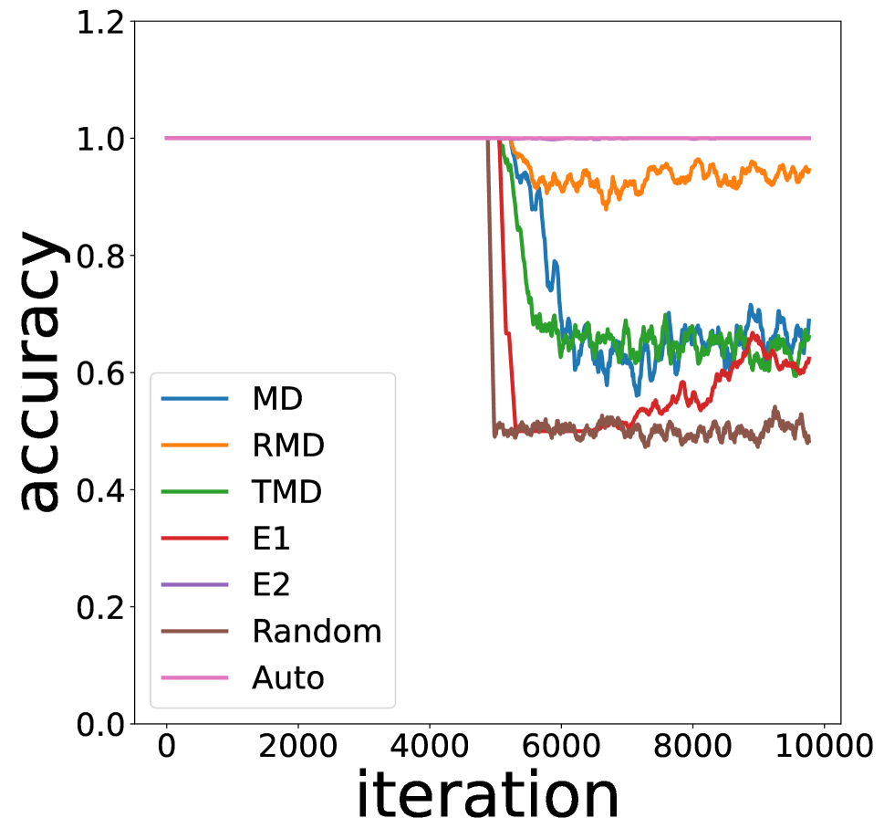
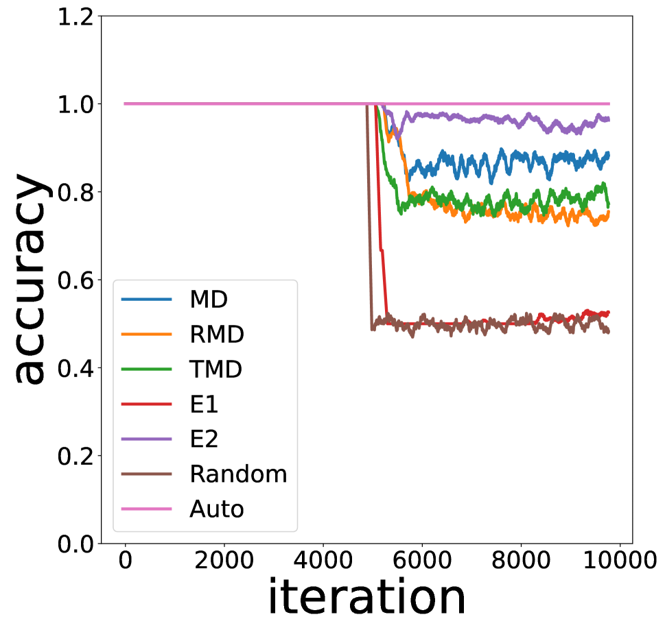
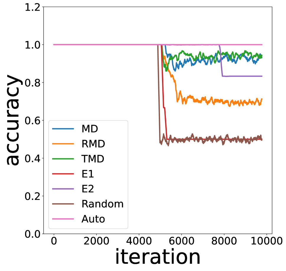
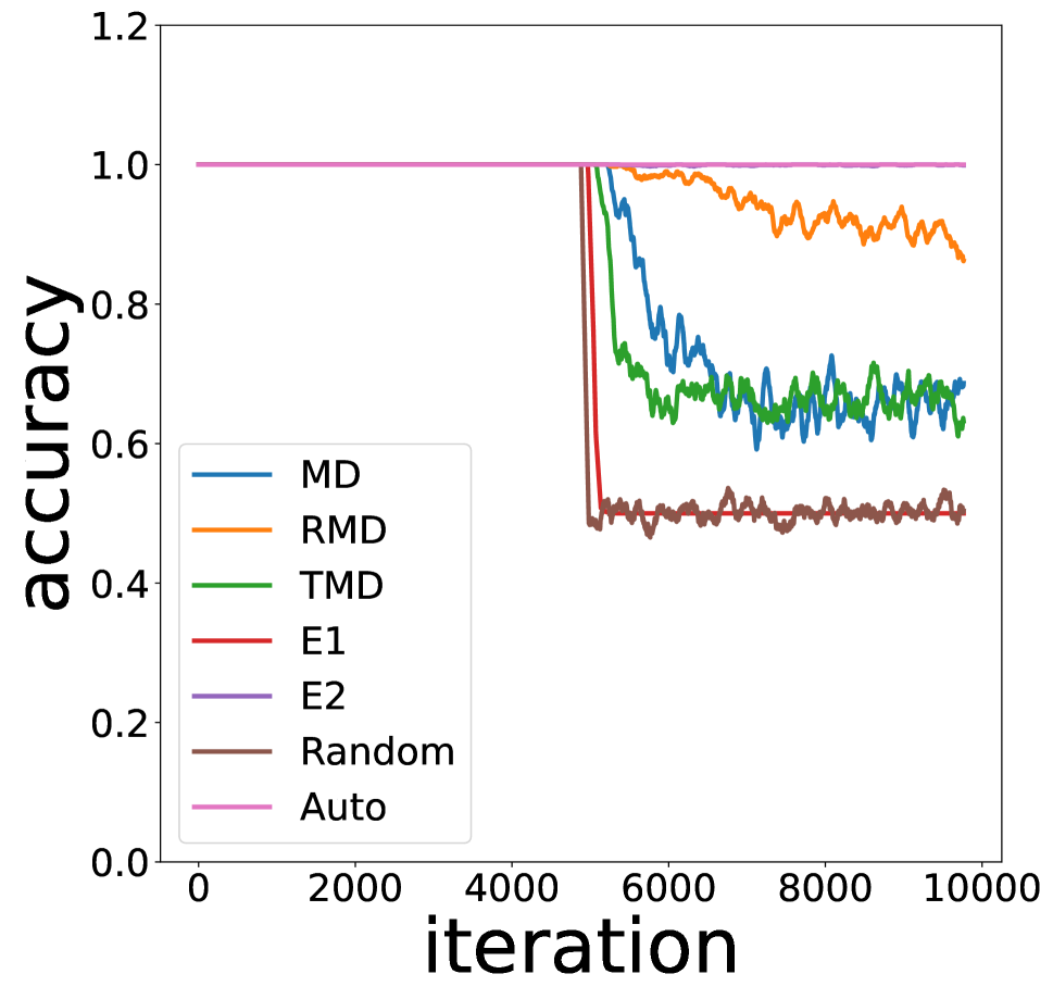
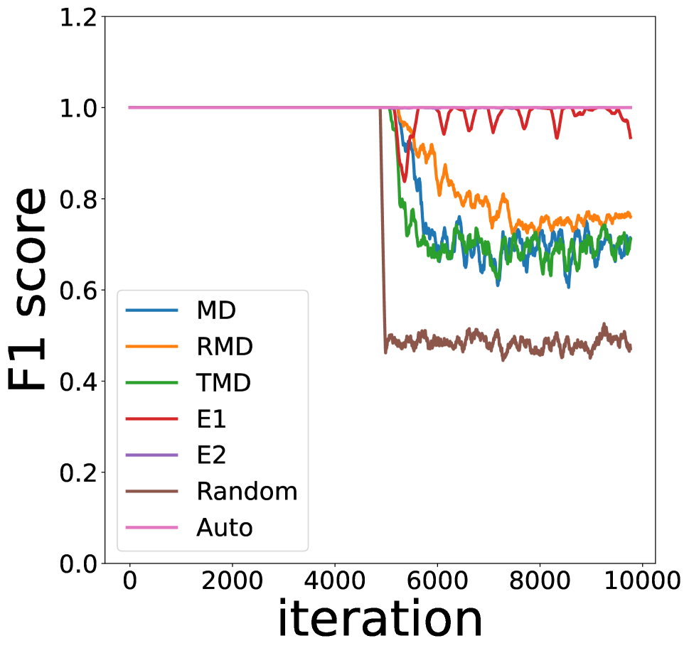
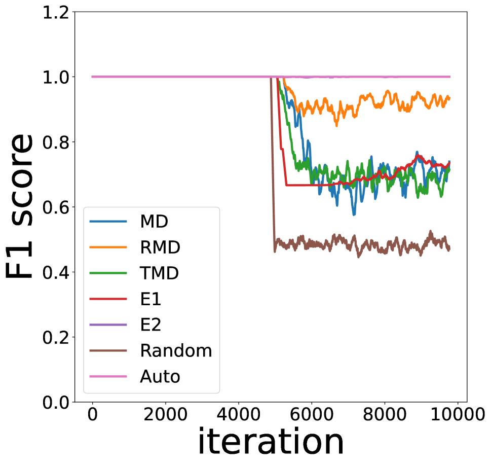
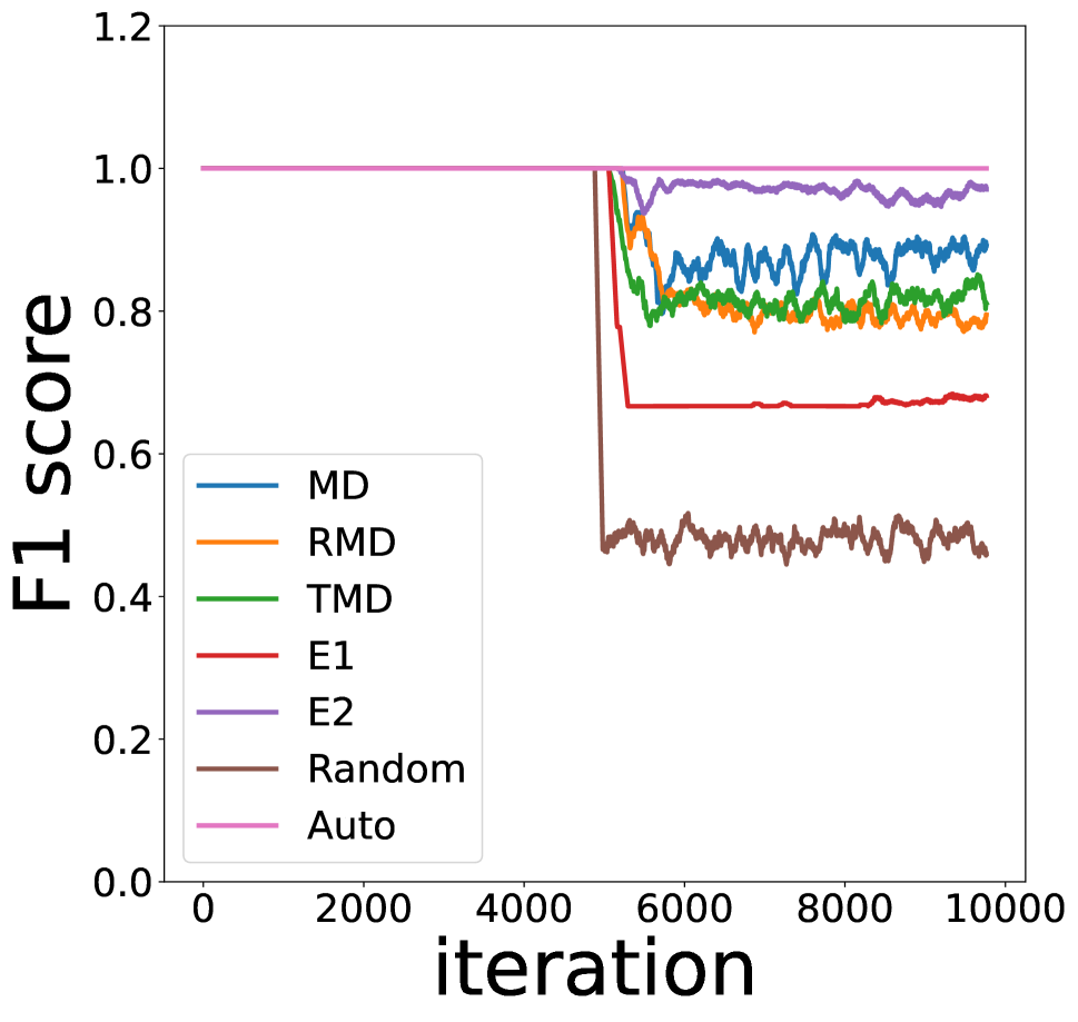
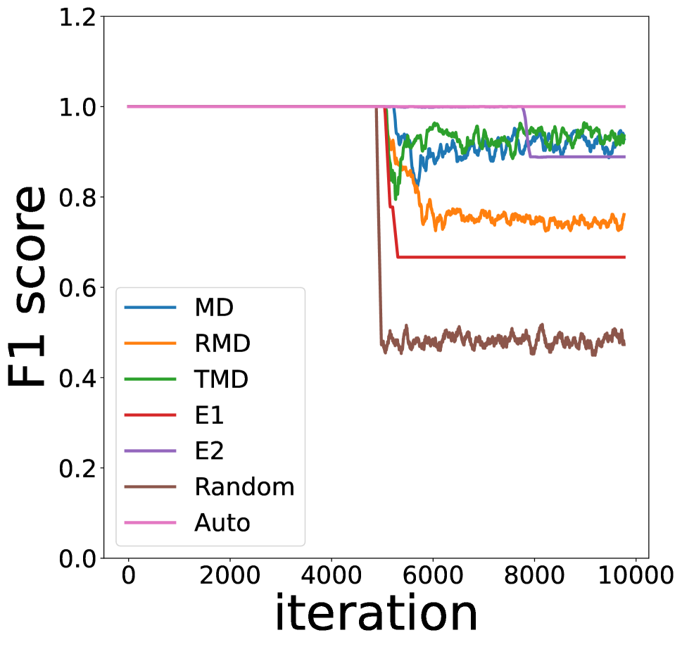
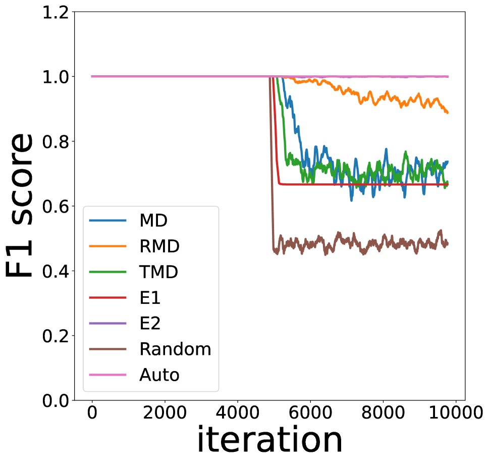
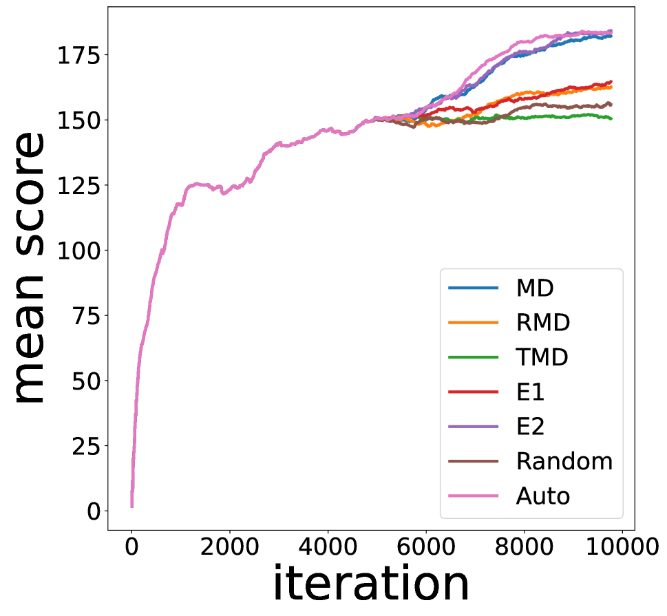
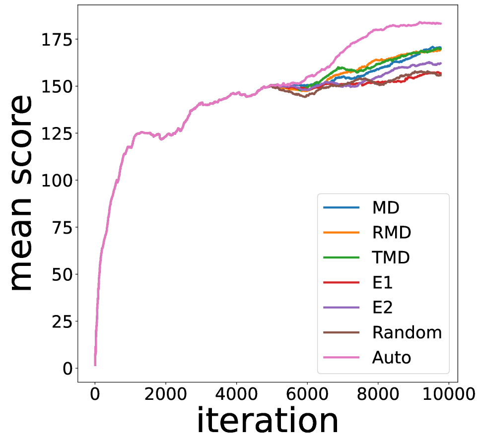
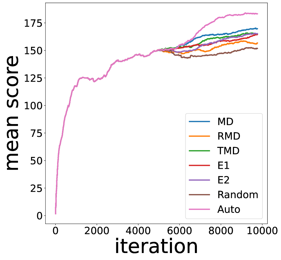
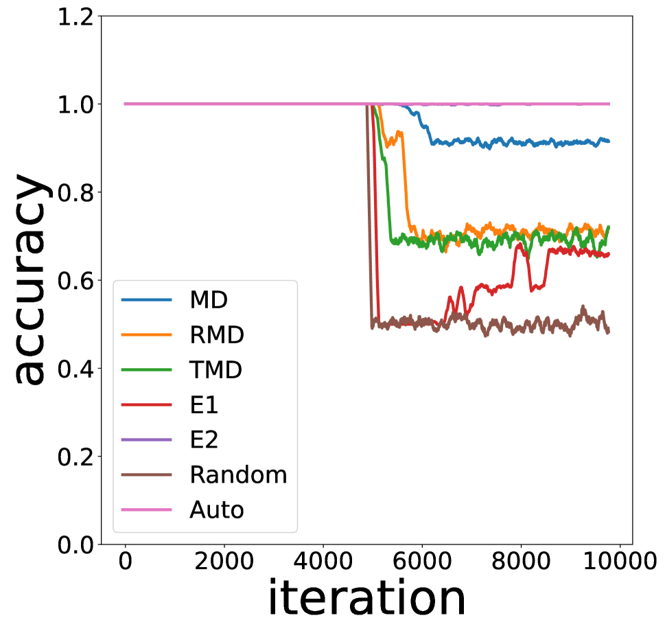
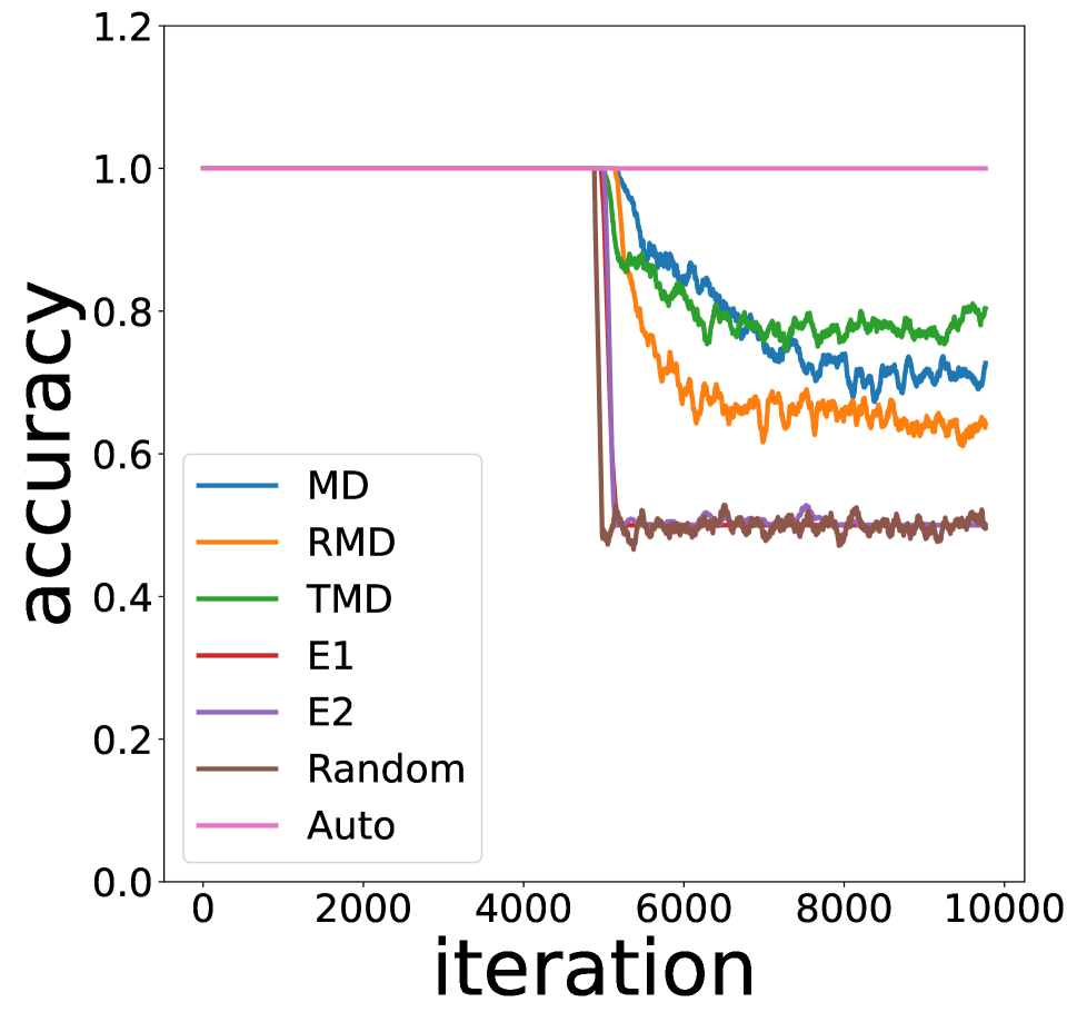
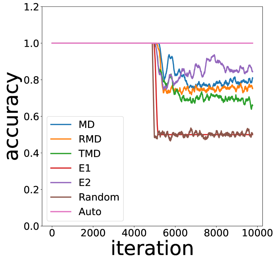
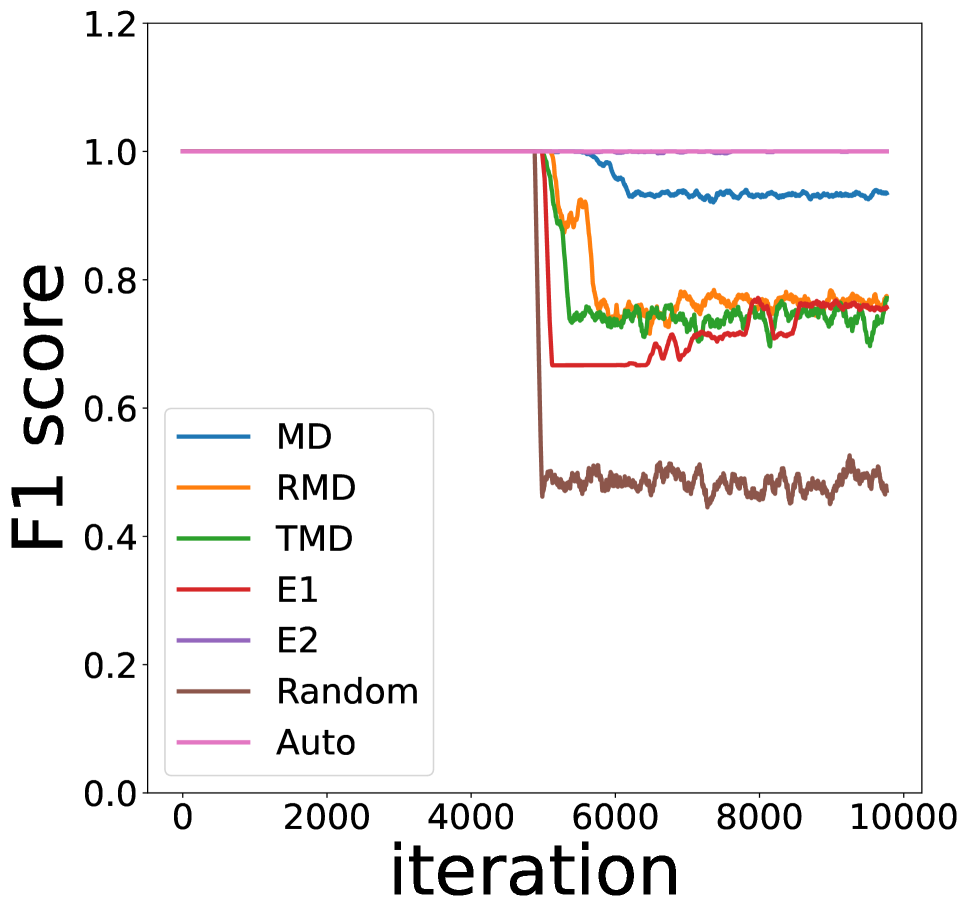
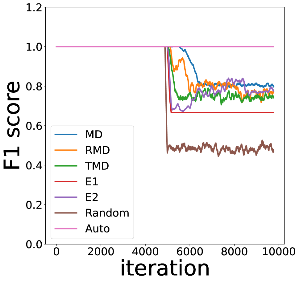
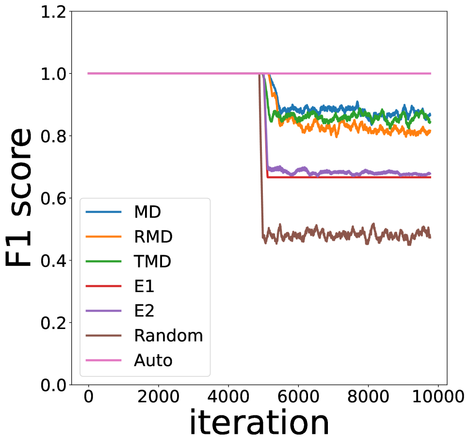
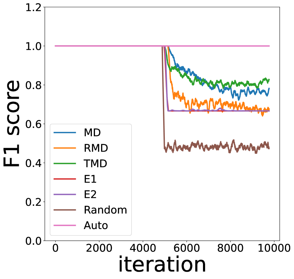
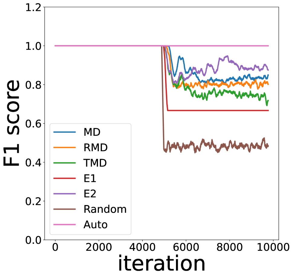
Main Results. In Figure 4, we shows the learning curves of cumulative rewards (first row) based on PPO algorithm and corresponding detection accuracy (second row) of different detection methods across different types of outliers on Tutankham games. We also provide the similar results on all six Atari games in Appendix F from Figures 16 to 21. Based on these results, we conclude that:
-
•
In general, E2, MD and RMD perform best or achieve competitive detection performance across different types of outliers, verifying the importance of using partial or full covariance information in the detector design compared with E1. By contrast, TMD is slightly inferior to MD and RMD, which justifies that the “tied” covariance assumption may be implausible in some cases.
-
•
The superiority of MD and RMD in the training phase may not be consistent to the evaluation phase. Specifically, under certain outlier circumstances, MD and RMD do not outperform E2. This may be caused by the noisy estimation of covariance matrix in the challenging online learning setting. MD strategy tends to outperform RMD in some cases, which may result from the information loss in the dimension reduction of the feature vectors for RMD in order to compromise its computation burden.
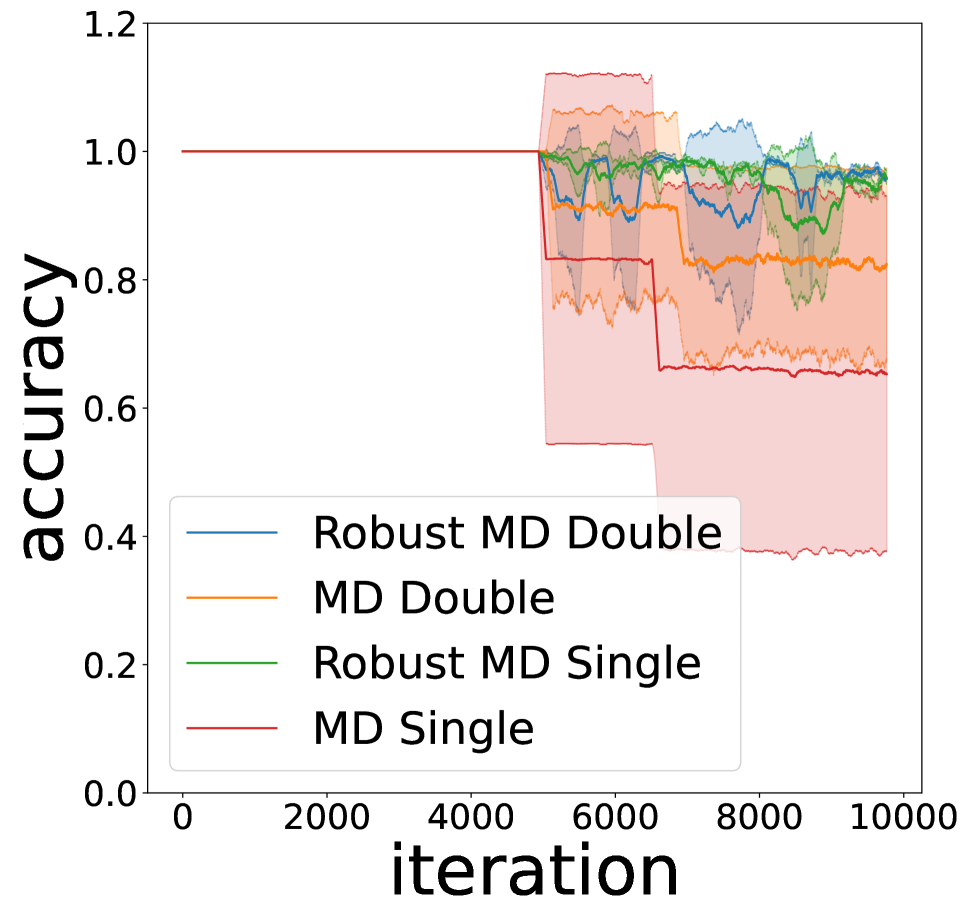
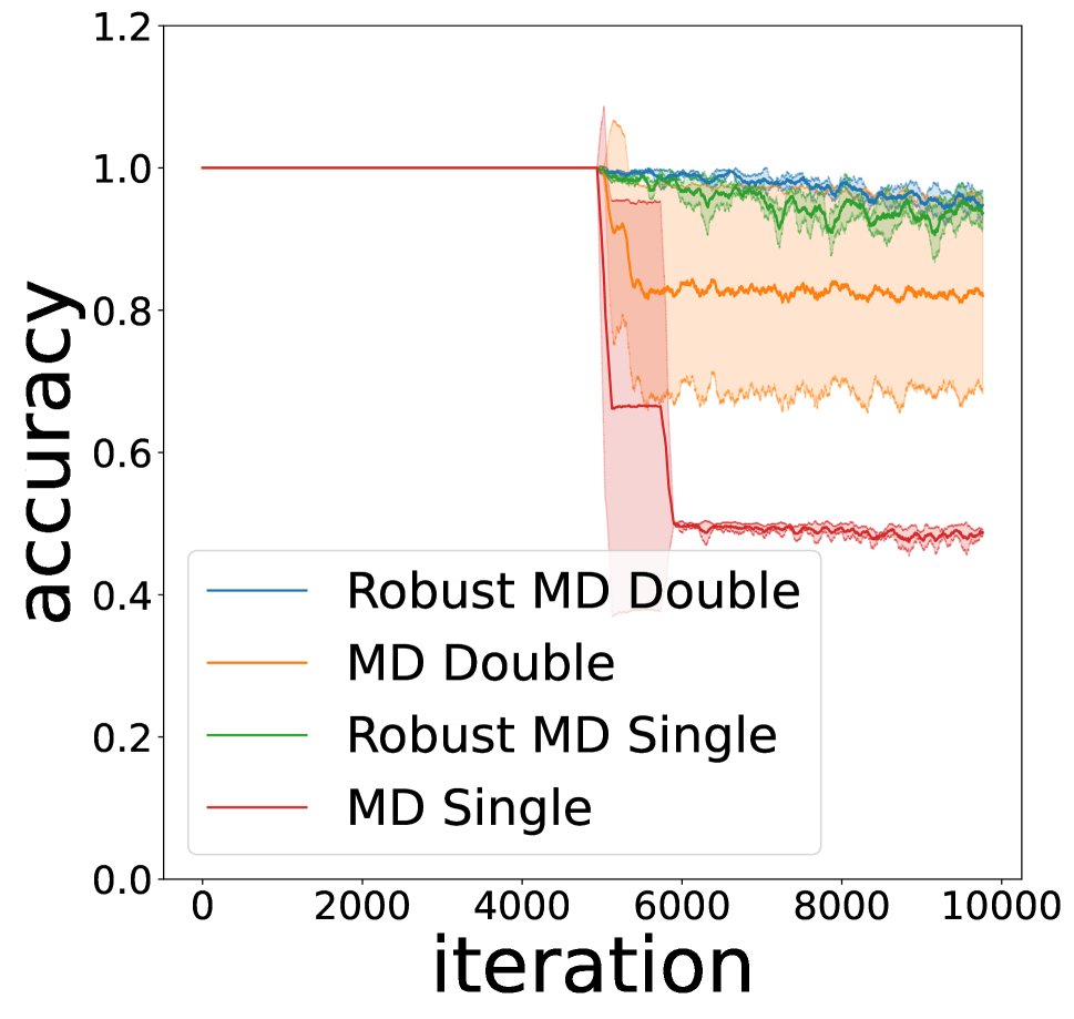
Ablation Study on Double Self-Supervised Detectors. We conduct an ablation study of double self-supervised detectors on Breakout games with random and OOD outliers. Figure 14 in Appendix F reveals that compared with the single detector, double self-supervised detectors can help to adjust the detection errors and improve the detection accuracy. MD with double detectors outperforms MD with single detector significantly, although RMD with double detectors is comparable to RMD with single detector.
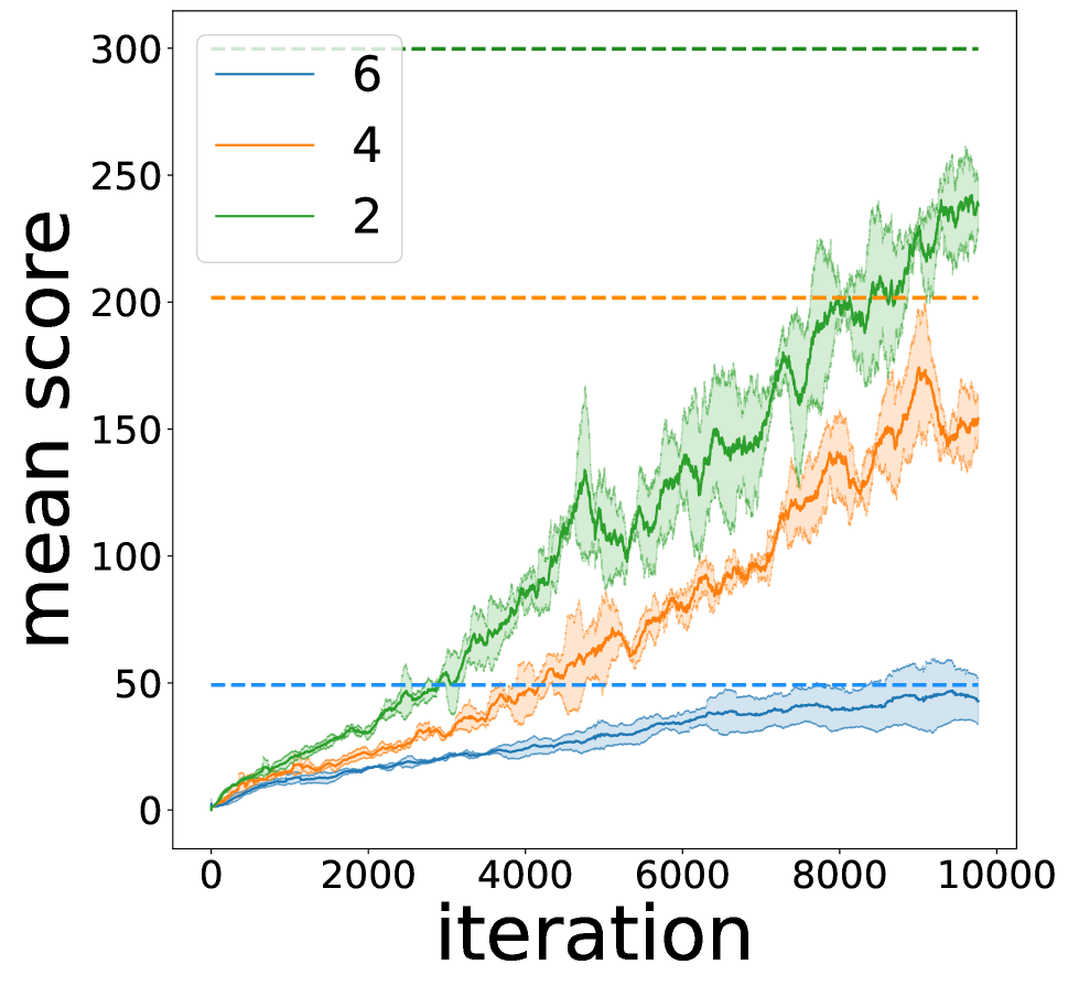
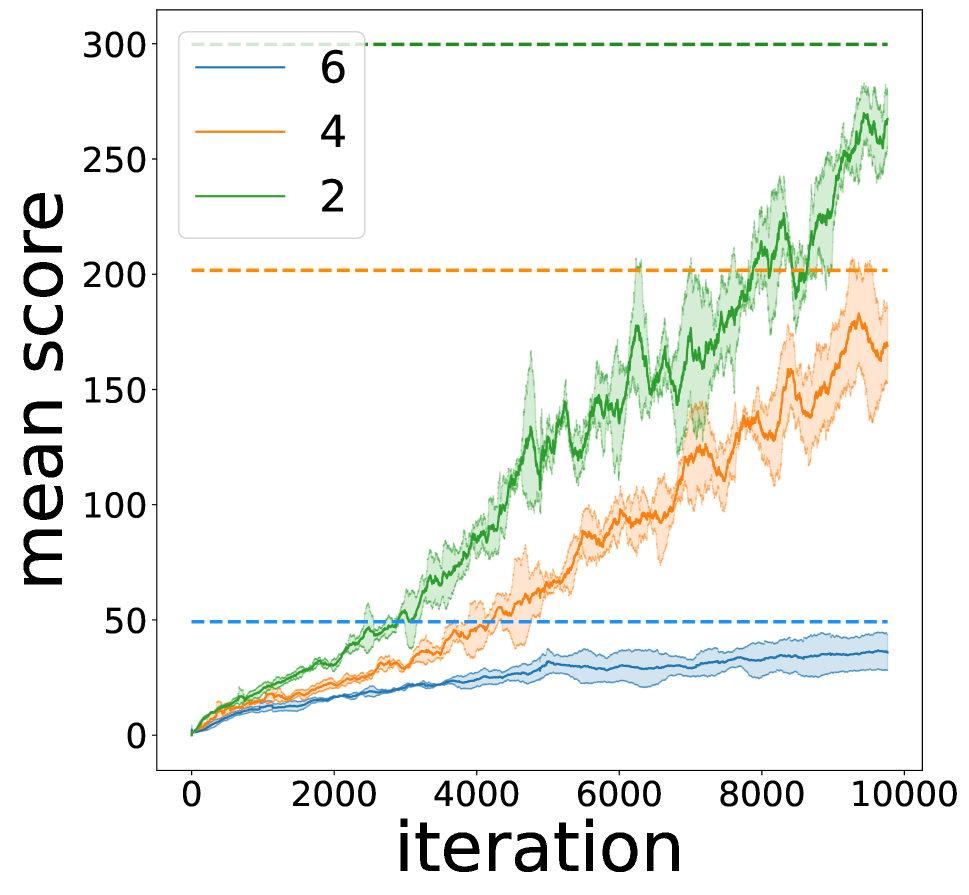
Ablation Study on Contamination Ratios. We study different contamination ratios that the agent encounters in the training phase. We train PPO in two, four or six noisy environments among all eight parallel environments with random and OOD outliers. We use PCA to reduce the feature vectors to 50 dimensions and estimate the detector using Robust MD. Figure 15 in Appendix F illustrates that comparing with the Auto baseline, our RMD method is robust when encountering different ratios of outliers, especially with a higher the contamination ratio.
7 Conclusion
In this paper, we propose a simple yet effective outlier detection framework in both the evaluation and training phases of RL by using Mahalanobis distance and robust Mahalanobis distance. Our proposed detection framework is generic, as it simultaneously considers random, adversarial and out-of-distribution states. Rigorous experiments demonstrate the efficacy of our detection strategies in contrast to other baseline methods. Our research is a contribution towards trustworthy deployment of RL algorithms in safety-critical cases.
References
- Abdi and Williams (2010) Abdi, H.; and Williams, L. J. 2010. Principal component analysis. Wiley interdisciplinary reviews: computational statistics, 2(4): 433–459.
- Bellemare et al. (2013) Bellemare, M. G.; Naddaf, Y.; Veness, J.; and Bowling, M. 2013. The Arcade Learning Environment: An Evaluation Platform for General Agents. Journal of Artificial Intelligence Research, 47: 253–279.
- Brockman et al. (2016) Brockman, G.; Cheung, V.; Pettersson, L.; Schneider, J.; Schulman, J.; Tang, J.; and Zaremba, W. 2016. OpenAI Gym. arXiv preprint arXiv:1606.01540.
- Butler, Davies, and Jhun (1993) Butler, R.; Davies, P.; and Jhun, M. 1993. Asymptotics for the minimum covariance determinant estimator. The Annals of Statistics, 1385–1400.
- Cabana, Lillo, and Laniado (2021) Cabana, E.; Lillo, R. E.; and Laniado, H. 2021. Multivariate outlier detection based on a robust Mahalanobis distance with shrinkage estimators. Statistical Papers, 62(4): 1583–1609.
- Cao et al. (2020) Cao, Y.; Chen, X.; Yao, L.; Wang, X.; and Zhang, W. E. 2020. Adversarial attacks and detection on reinforcement learning-based interactive recommender systems. In Proceedings of the 43rd International ACM SIGIR Conference on Research and Development in Information Retrieval, 1669–1672.
- Chan et al. (2019) Chan, S. C.; Fishman, S.; Canny, J.; Korattikara, A.; and Guadarrama, S. 2019. Measuring the reliability of reinforcement learning algorithms. International Conference on Learning Representations (ICLR).
- Colas, Sigaud, and Oudeyer (2018) Colas, C.; Sigaud, O.; and Oudeyer, P.-Y. 2018. How many random seeds? Statistical power analysis in deep reinforcement learning experiments. arXiv preprint arXiv:1806.08295.
- De Maesschalck, Jouan-Rimbaud, and Massart (2000) De Maesschalck, R.; Jouan-Rimbaud, D.; and Massart, D. L. 2000. The Mahalanobis distance. Chemometrics and Intelligent Laboratory Systems, 50(1): 1–18.
- Goodfellow, Shlens, and Szegedy (2014) Goodfellow, I. J.; Shlens, J.; and Szegedy, C. 2014. Explaining and harnessing adversarial examples. International Conference on Learning Representations (ICLR).
- Greenberg and Mannor (2021) Greenberg, I.; and Mannor, S. 2021. Detecting rewards deterioration in episodic reinforcement learning. In International Conference on Machine Learning, 3842–3853. PMLR.
- Grübel (1988) Grübel, R. 1988. A minimal characterization of the covariance matrix. Metrika, 35(1): 49–52.
- Hardin and Rocke (2005) Hardin, J.; and Rocke, D. M. 2005. The distribution of robust distances. Journal of Computational and Graphical Statistics, 14(4): 928–946.
- Hastie et al. (2009) Hastie, T.; Tibshirani, R.; Friedman, J. H.; and Friedman, J. H. 2009. The elements of statistical learning: data mining, inference, and prediction, volume 2. Springer.
- Henderson et al. (2018) Henderson, P.; Islam, R.; Bachman, P.; Pineau, J.; Precup, D.; and Meger, D. 2018. Deep reinforcement learning that matters. In Proceedings of the AAAI Conference on Artificial Intelligence, volume 32.
- Hessel et al. (2018) Hessel, M.; Modayil, J.; Van Hasselt, H.; Schaul, T.; Ostrovski, G.; Dabney, W.; Horgan, D.; Piot, B.; Azar, M.; and Silver, D. 2018. Rainbow: Combining improvements in deep reinforcement learning. In Thirty-second AAAI conference on artificial intelligence.
- Huang et al. (2017) Huang, S.; Papernot, N.; Goodfellow, I.; Duan, Y.; and Abbeel, P. 2017. Adversarial attacks on neural network policies. Advances in Neural Information Processing Systems.
- Huber (2004) Huber, P. J. 2004. Robust statistics, volume 523. John Wiley & Sons.
- Jordan et al. (2020) Jordan, S.; Chandak, Y.; Cohen, D.; Zhang, M.; and Thomas, P. 2020. Evaluating the performance of reinforcement learning algorithms. In International Conference on Machine Learning, 4962–4973. PMLR.
- Kamoi and Kobayashi (2020) Kamoi, R.; and Kobayashi, K. 2020. Why is the Mahalanobis distance effective for anomaly detection. arXiv preprint arXiv:2003.00402.
- Klecka, Iversen, and Klecka (1980) Klecka, W. R.; Iversen, G. R.; and Klecka, W. R. 1980. Discriminant analysis, volume 19. Sage.
- Lee et al. (2018) Lee, K.; Lee, K.; Lee, H.; and Shin, J. 2018. A simple unified framework for detecting out-of-distribution samples and adversarial attacks. Advances in Neural Information Processing Systems, 31.
- Lillicrap et al. (2015) Lillicrap, T. P.; Hunt, J. J.; Pritzel, A.; Heess, N.; Erez, T.; Tassa, Y.; Silver, D.; and Wierstra, D. 2015. Continuous control with deep reinforcement learning. arXiv preprint arXiv:1509.02971.
- Maronna and Yohai (2014) Maronna, R. A.; and Yohai, V. J. 2014. Robust estimation of multivariate location and scatter. Wiley StatsRef: Statistics Reference Online, 1–12.
- Mnih et al. (2016) Mnih, V.; Badia, A. P.; Mirza, M.; Graves, A.; Lillicrap, T.; Harley, T.; Silver, D.; and Kavukcuoglu, K. 2016. Asynchronous methods for deep reinforcement learning. In International conference on machine learning, 1928–1937. PMLR.
- Mnih et al. (2015) Mnih, V.; Kavukcuoglu, K.; Silver, D.; Rusu, A. A.; Veness, J.; Bellemare, M. G.; Graves, A.; Riedmiller, M.; Fidjeland, A. K.; Ostrovski, G.; et al. 2015. Human-level control through deep reinforcement learning. Nature, 518(7540): 529–533.
- Pang et al. (2021) Pang, G.; Shen, C.; Cao, L.; and Hengel, A. V. D. 2021. Deep learning for anomaly detection: A review. ACM Computing Surveys (CSUR), 54(2): 1–38.
- Pattanaik et al. (2017) Pattanaik, A.; Tang, Z.; Liu, S.; Bommannan, G.; and Chowdhary, G. 2017. Robust deep reinforcement learning with adversarial attacks. Advances in Neural Information Processing Systems.
- Ren et al. (2021) Ren, J.; Fort, S.; Liu, J.; Roy, A. G.; Padhy, S.; and Lakshminarayanan, B. 2021. A simple fix to Mahalanobis distance for improving near-OOD detection. arXiv preprint arXiv:2106.09022.
- Rousseeuw (1984) Rousseeuw, P. J. 1984. Least median of squares regression. Journal of the American Statistical Association, 79(388): 871–880.
- Rousseeuw and Driessen (1999) Rousseeuw, P. J.; and Driessen, K. V. 1999. A fast algorithm for the minimum covariance determinant estimator. Technometrics, 41(3): 212–223.
- Rousseeuw and Van Zomeren (1990) Rousseeuw, P. J.; and Van Zomeren, B. C. 1990. Unmasking multivariate outliers and leverage points. Journal of the American Statistical Association, 85(411): 633–639.
- Schulman et al. (2015a) Schulman, J.; Levine, S.; Abbeel, P.; Jordan, M.; and Moritz, P. 2015a. Trust region policy optimization. In Proceedings of The 32nd International Conference on Machine Learning, 1889–1897. PMLR.
- Schulman et al. (2015b) Schulman, J.; Moritz, P.; Levine, S.; Jordan, M.; and Abbeel, P. 2015b. High-dimensional continuous control using generalized advantage estimation. arXiv preprint arXiv:1506.02438.
- Schulman et al. (2017) Schulman, J.; Wolski, F.; Dhariwal, P.; Radford, A.; and Klimov, O. 2017. Proximal policy optimization algorithms. arXiv preprint arXiv:1707.06347.
- Sutton and Barto (2018) Sutton, R. S.; and Barto, A. G. 2018. Reinforcement learning: An introduction. MIT press.
- Szegedy et al. (2013) Szegedy, C.; Zaremba, W.; Sutskever, I.; Bruna, J.; Erhan, D.; Goodfellow, I.; and Fergus, R. 2013. Intriguing properties of neural networks. International Conference on Learning Representations (ICLR).
- Todorov, Erez, and Tassa (2012) Todorov, E.; Erez, T.; and Tassa, Y. 2012. Mujoco: A physics engine for model-based control. In 2012 IEEE/RSJ International Conference on Intelligent Robots and Systems, 5026–5033. IEEE.
- Wilson and Hilferty (1931) Wilson, E. B.; and Hilferty, M. M. 1931. The distribution of chi-square. Proceedings of the National Academy of Sciences of the United States of America, 17(12): 684.
Appendix A Proof of Proposition 1
Proof.
We show that for each action class , the square of Mahalanobis distance is identically independent Chi-squared distributed under Gaussian assumption. Without loss of generality, we denote and as the mean and variance matrix of the closest class-conditional Gaussian distribution. We need to show is Chi-squared distributed. Firstly, by eigenvalue decomposition, we have
| (5) |
where and are the -th eigenvalue and eigenvector of . Plugging it into the form of , we immediately obtain
| (6) | ||||
where is a new Gaussian variable that results from the linear transform of a Gaussian distribution where . Therefore, the resulting variance can be derived as
| (7) | ||||
As the and are orthogonal if , the variance can be further reduced to
| (8) | ||||
Each is a standard Gaussian distribution. Then we have , the square of Mahalanobis distance, is Chi-squared distributed, i.e., , which is independent of the action class . Without loss of generality, the smallest over all action classes, i.e., , is also a Chi-squared distribution. That is to say, .
∎
Appendix B Evaluation Phase: Main Results
| Accuracy (%) | Outliers | Strength | MD/Robust MD (=0.0) | MD/Robust MD (=0.01) | MD/Robust MD (=0.1) | ||||||
| =0.01 | =0.05 | =0.1 | =0.01 | =0.05 | =0.1 | =0.01 | =0.05 | =0.1 | |||
| Breakout | Random | std=0.02 | 51.8/64.7 | 52.4/66.0 | 52.5/66.6 | 50.3/62.1 | 50.4/63.8 | 50.4/64.6 | 49.3/46.6 | 48.7/46.2 | 48.3/45.9 |
| std=0.04 | 63.0/88.7 | 64.8/88.7 | 65.7/88.4 | 53.8/66.1 | 54.8/69.1 | 55.5/70.7 | 49.3/49.6 | 48.7/49.0 | 48.2/48.7 | ||
| std=0.06 | 88.8/91.6 | 91.8/89.8 | 93.2/88.8 | 62.2/94.1 | 67.0/92.7 | 70.2/91.7 | 49.7/55.3 | 49.4/56.0 | 49.2/56.4 | ||
| Adversarial | =0.001 | 85.8/89.4 | 88.6/89.3 | 89.7/88.8 | 82.6/89.1 | 85.6/89.3 | 87.1/89.2 | 73.4/88.1 | 77.7/89.0 | 80.1/89.0 | |
| =0.01 | 94.3/93.6 | 95.1/91.4 | 95.3/90.5 | 91.3/92.1 | 93.4/90.9 | 94.1/90.1 | 77.5/92.2 | 82.3/91.4 | 84.7/90.6 | ||
| =0.05 | 99.1/93.9 | 98.4/92.3 | 97.8/91.2 | 99.6/94.1 | 99.1/92.7 | 98.8/91.7 | 74.3/95.2 | 81.2/94.0 | 84.8/92.9 | ||
| OOD | Asterix | 50.5/73.8 | 50.6/87.9 | 50.4/89.1 | 50.2/48.8 | 49.8/48.3 | 49.5/48.0 | 49.7/44.7 | 49.0/43.5 | 48.4/42.6 | |
| SpaceInvaders | 50.7/91.9 | 50.5/91.8 | 50.3/91.3 | 49.8/54.3 | 49.5/56.9 | 49.2/58.8 | 49.5/44.5 | 48.9/43.2 | 48.3/42.2 | ||
| Asterix | Random | std=0.1 | 49.8/54.3 | 49.8/56.5 | 49.7/57.8 | 49.8/54.2 | 49.8/56.1 | 49.7/57.3 | 49.8/50.9 | 49.8/51.4 | 49.7/51.6 |
| std=0.15 | 50.1/79.4 | 50.2/83.1 | 50.2/84.8 | 50.2/83.4 | 50.2/87.7 | 50.2/89.6 | 49.8/50.7 | 49.8/51.4 | 49.7/51.9 | ||
| std=0.2 | 53.9/95.0 | 56.4/94.7 | 58.5/94.4 | 51.1/95.1 | 51.7/94.8 | 52.3/94.4 | 49.9/52.8 | 49.9/54.8 | 49.8/56.3 | ||
| Adversarial | =0.001 | 85.5/91.7 | 87.6/92.1 | 88.3/92.5 | 81.1/92.2 | 83.9/92.8 | 85.4/92.6 | 64.0/85.5 | 69.5/86.2 | 72.7/86.6 | |
| =0.01 | 88.0/92.8 | 89.6/93.5 | 90.4/93.4 | 84.4/93.7 | 86.7/93.8 | 87.6/93.8 | 66.2/91.8 | 71.8/92.1 | 74.8/91.9 | ||
| =0.05 | 96.1/94.9 | 96.9/94.6 | 97.2/94.4 | 93.6/95.1 | 94.8/94.7 | 95.3/94.4 | 76.5/95.6 | 81.6/95.4 | 84.1/95.1 | ||
| OOD | Breakout | 50.1/95.0 | 49.8/94.7 | 49.7/94.4 | 50.1/45.6 | 50.0/45.1 | 49.8/44.9 | 50.1/44.4 | 49.9/43.3 | 49.7/42.6 | |
| SpaceInvaders | 49.5/46.0 | 49.3/46.3 | 49.1/46.6 | 49.5/46.5 | 49.3/46.4 | 49.2/46.4 | 49.5/44.4 | 49.2/43.6 | 49.0/42.9 | ||
| SpaceInvaders | Random | std=0.02 | 50.2/65.3 | 50.5/71.6 | 50.8/75.1 | 50.2/59.6 | 50.5/64.5 | 50.7/68.1 | 49.9/50.3 | 49.9/50.7 | 49.8/51.0 |
| std=0.04 | 67.8/97.3 | 73.6/96.8 | 77.1/96.3 | 57.0/96.5 | 61.5/95.8 | 64.5/95.3 | 49.9/52.1 | 49.9/53.1 | 49.9/53.9 | ||
| std=0.06 | 92.7/98.2 | 95.9/97.4 | 96.7/95.9 | 70.1/96.3 | 77.8/95.5 | 82.5/94.9 | 52.1/62.8 | 50.3/66.6 | 50.6/69.3 | ||
| Adversarial | =0.001 | 92.3/96.4 | 94.8/96.0 | 95.9/95.6 | 90.4/95.4 | 93.5/94.9 | 94.8/94.6 | 70.9/91.6 | 77.8/92.8 | 81.2/92.6 | |
| =0.01 | 97.0/97.7 | 97.9/97.0 | 98.2/96.4 | 94.8/96.3 | 96.7/95.6 | 97.3/95.1 | 74.0/97.9 | 81.5/97.3 | 85.4/96.7 | ||
| =0.05 | 99.8/97.5 | 99.7/96.7 | 99.5/96.0 | 99.9/96.5 | 99.7/95.7 | 99.6/95.2 | 86.9/98.3 | 92.6/97.6 | 94.5/97.0 | ||
| OOD | Breakout | 50.4/61.8 | 50.2/69.3 | 50.0/73.6 | 50.3/77.3 | 50.1/78.7 | 50.0/79.8 | 50.2/46.4 | 50.0/45.3 | 49.8/44.5 | |
| Asterix | 51.1/97.8 | 54.4/97.0 | 59.3/96.2 | 50.1/96.6 | 49.9/95.8 | 49.8/95.1 | 49.9/45.8 | 49.7/44.5 | 49.6/43.5 | ||
| Accuracy (%) | Outliers | Strength | MD/Robust MD (=0.0) | MD/Robust MD (=0.01) | MD/Robust MD (=0.1) | ||||||
| =0.01 | =0.05 | =0.1 | =0.01 | =0.05 | =0.1 | =0.01 | =0.05 | =0.1 | |||
| Enduro | Random | std=0.1 | 49.8/73.3 | 49.7/79.5 | 49.7/82.6 | 49.8/73.3 | 49.8/79.7 | 49.9/82.7 | 49.7/51.2 | 49.6/53.0 | 49.6/54.2 |
| std=0.2 | 51.5/95.8 | 53.4/95.4 | 55.3/95.1 | 52.3/97.3 | 55.2/96.9 | 58.2/96.7 | 49.8/73.7 | 49.8/81.7 | 49.8/85.7 | ||
| std=0.3 | 76.4/95.8 | 87.0/95.4 | 91.5/95.0 | 73.3/97.3 | 85.0/96.9 | 90.0/96.6 | 50.5/97.3 | 51.1/96.9 | 51.7/96.6 | ||
| Adversarial | =0.001 | 99.5/96.5 | 99.4/96.1 | 99.3/95.8 | 98.2/95.9 | 99.2/95.5 | 99.3/95.2 | 59.7/97.9 | 66.2/97.7 | 70.6/97.4 | |
| =0.01 | 99.5/96.5 | 99.4/96.1 | 99.3/95.8 | 99.5/95.9 | 99.5/95.5 | 99.4/95.1 | 62.9/97.9 | 70.5/97.6 | 75.7/97.3 | ||
| =0.05 | 99.5/96.6 | 99.4/96.2 | 99.3/95.9 | 99.7/95.9 | 99.5/95.5 | 99.4/95.2 | 77.8/98.0 | 86.8/97.6 | 91.1/97.4 | ||
| OOD | FishingDerby | 59.4/96.4 | 69.6/96.0 | 76.7/95.8 | 52.7/95.9 | 56.1/95.5 | 59.7/95.1 | 49.8/56.5 | 49.8/59.8 | 49.9/61.8 | |
| Tutankham | 51.2/96.4 | 53.1/96.0 | 55.2/95.8 | 50.5/95.9 | 50.8/95.5 | 51.1/95.1 | 49.9/50.2 | 49.9/50.8 | 49.8/51.2 | ||
| FishingDerby | Random | std=0.1 | 50.0/50.1 | 49.9/50.3 | 49.9/50.4 | 50.0/50.0 | 50.0/50.0 | 49.9/50.2 | 49.9/49.8 | 49.8/49.7 | 49.9/49.7 |
| std=0.2 | 50.1/78.9 | 50.2/89.3 | 50.3/93.4 | 50.1/68.2 | 50.2/81.3 | 50.3/87.6 | 50.0/50.7 | 50.0/51.0 | 49.9/51.3 | ||
| std=0.3 | 57.2/99.3 | 63.7/99.1 | 69.8/98.9 | 52.0/99.2 | 53.4/99.0 | 54.9/98.9 | 50.2/63.3 | 50.3/71.2 | 50.4/75.5 | ||
| Adversarial | =0.001 | 98.7/99.3 | 99.2/99.1 | 99.4/98.9 | 94.6/99.2 | 97.8/99.0 | 98.4/98.9 | 59.6/99.3 | 66.3/99.1 | 71.8/98.9 | |
| =0.01 | 99.5/99.2 | 99.7/99.0 | 99.8/98.8 | 98.3/99.2 | 99.3/99.0 | 99.5/98.8 | 66.6/99.3 | 77.3/99.0 | 83.6/98.9 | ||
| =0.05 | 99.9/99.2 | 99.9/99.0 | 99.8/98.8 | 99.9/99.2 | 99.9/99.0 | 99.9/98.8 | 90.7/99.2 | 96.9/99.1 | 98.4/98.9 | ||
| OOD | Enduro | 50.1/75.8 | 50.1/91.4 | 50.1/96.3 | 50.0/49.7 | 49.9/49.6 | 49.8/49.5 | 49.9/49.4 | 49.9/49.1 | 49.8/48.9 | |
| Tutankham | 50.6/72.3 | 50.7/88.5 | 50.8/90.3 | 50.4/51.1 | 50.4/51.2 | 50.3/51.1 | 50.0/50.3 | 49.9/50.1 | 49.9/49.9 | ||
| Tutankham | Random | std=0.02 | 50.0/51.5 | 49.9/52.3 | 49.9/52.8 | 50.0/51.8 | 50.0/52.9 | 49.9/53.7 | 50.0/52.5 | 50.0/53.9 | 50.0/55.1 |
| std=0.04 | 49.9/74.1 | 49.8/80.7 | 49.8/83.9 | 49.9/67.8 | 49.9/73.0 | 49.8/76.4 | 49.9/67.6 | 49.9/73.7 | 49.8/77.4 | ||
| std=0.06 | 49.9/94.0 | 49.8/94.7 | 49.8/94.7 | 49.9/89.0 | 49.8/91.4 | 49.8/92.5 | 49.8/88.2 | 49.8/91.5 | 49.8/92.6 | ||
| Adversarial | =0.001 | 76.0/95.7 | 85.6/95.3 | 90.2/95.1 | 67.6/95.7 | 77.1/95.4 | 84.1/95.2 | 55.6/77.8 | 56.5/81.4 | 57.3/84.0 | |
| =0.01 | 95.9/95.7 | 98.4/95.3 | 98.6/95.1 | 91.5/95.8 | 95.7/95.5 | 96.9/95.2 | 57.2/95.6 | 58.7/95.6 | 60.0/95.4 | ||
| =0.05 | 99.4/95.5 | 99.1/95.2 | 99.0/95.0 | 99.5/95.9 | 99.4/95.5 | 99.3/95.3 | 66.6/95.9 | 71.6/95.6 | 73.9/95.4 | ||
| OOD | Enduro | 99.2/95.7 | 99.1/95.3 | 99.0/95.1 | 55.1/95.7 | 61.8/95.4 | 67.0/95.2 | 49.4/90.4 | 49.1/91.1 | 49.0/91.4 | |
| FishingDerby | 60.0/95.6 | 66.7/95.3 | 72.0/95.1 | 53.5/95.8 | 55.4/95.4 | 57.1/95.2 | 50.2/95.9 | 50.5/95.6 | 50.6/95.4 | ||
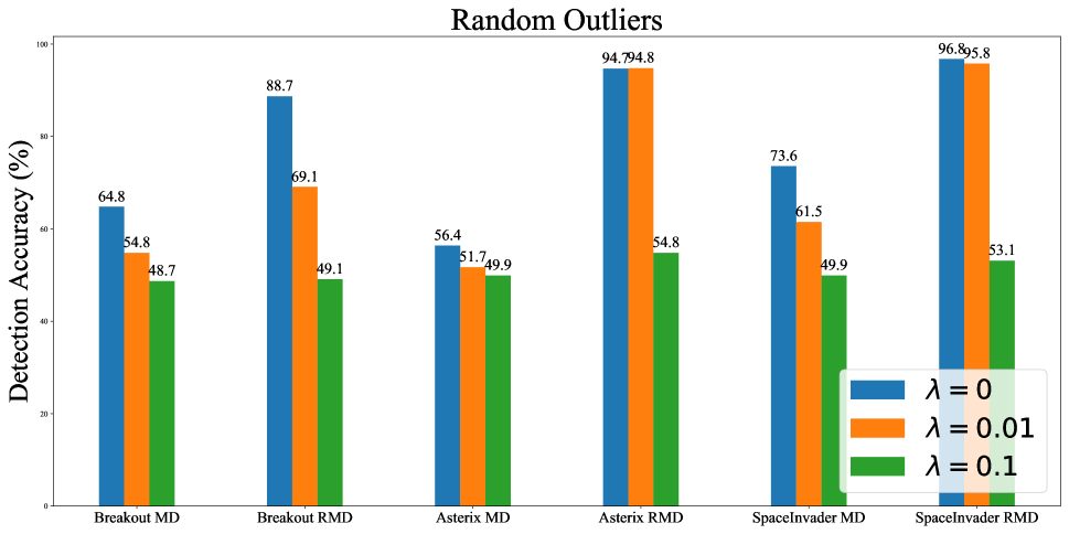
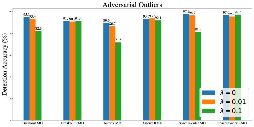
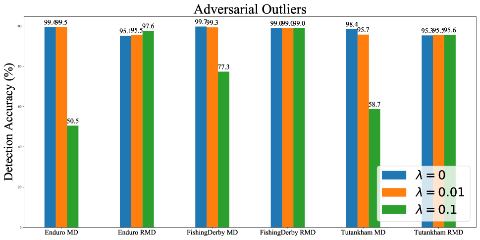
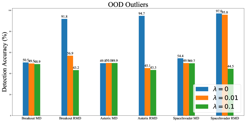
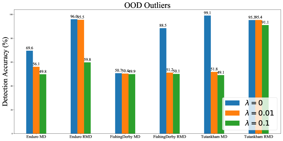
We provide the main result of our detection strategies on Breakout, Asterix, SpaceInvaders, Enduro, FishingDerby and Tutankham games in Tables 2 and 3 across different factions of contamination and significant level in the statistical test. We render detection accuracy of one detection method in bold that are 10 larger than the other detection method given the same and fraction of contamination, which we denote as . From the results in the two tables, it turns out that Robust MD-based detection method mostly outperforms classical MD detection method across different contamination ratio and is comparable in other cases.
We make a detailed comparison in Figures 5, 6 and 7. We can further conclude that (1) The effectiveness of both strategies tends to reduce as the proportion of contamination increases. (2) The superiority of robust MD-based detection against adversarial outliers is less sensitive to the increase of contamination ratio as opposed to MD-based detection method.
Appendix C Visualization of Outlier States on Six Games
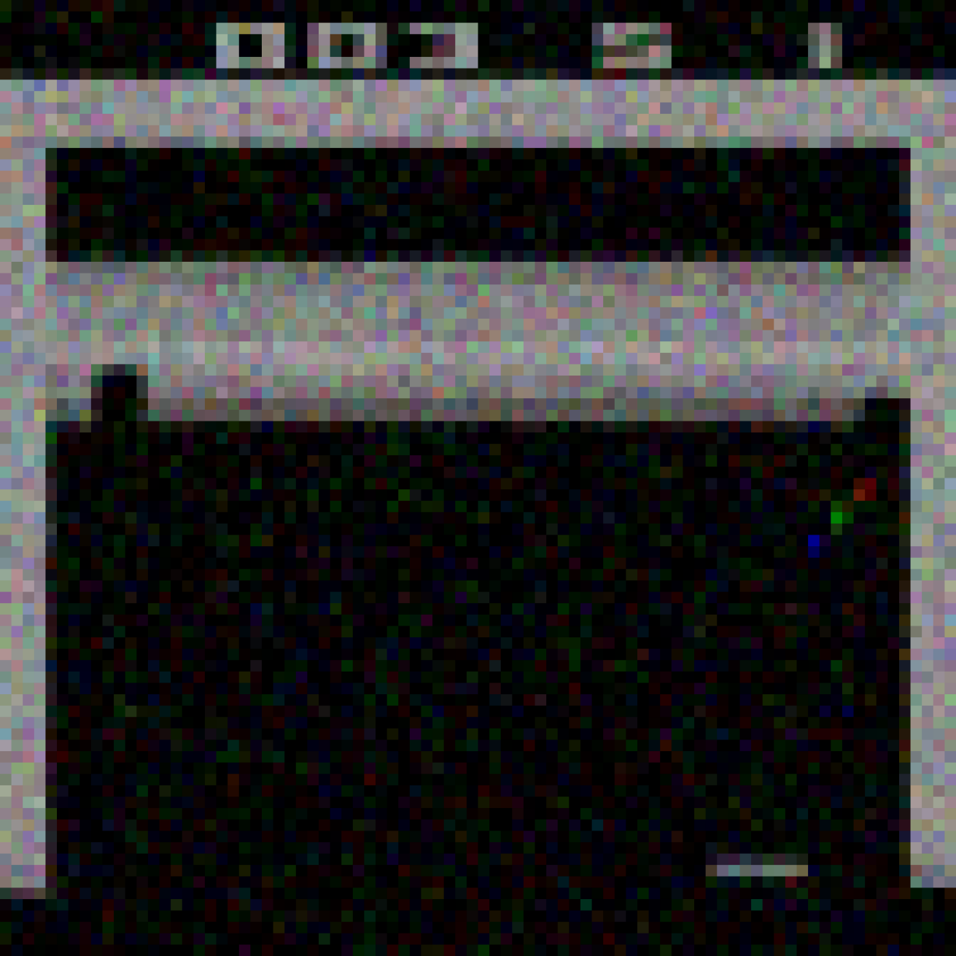
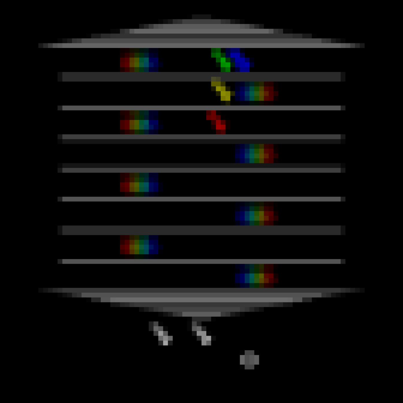
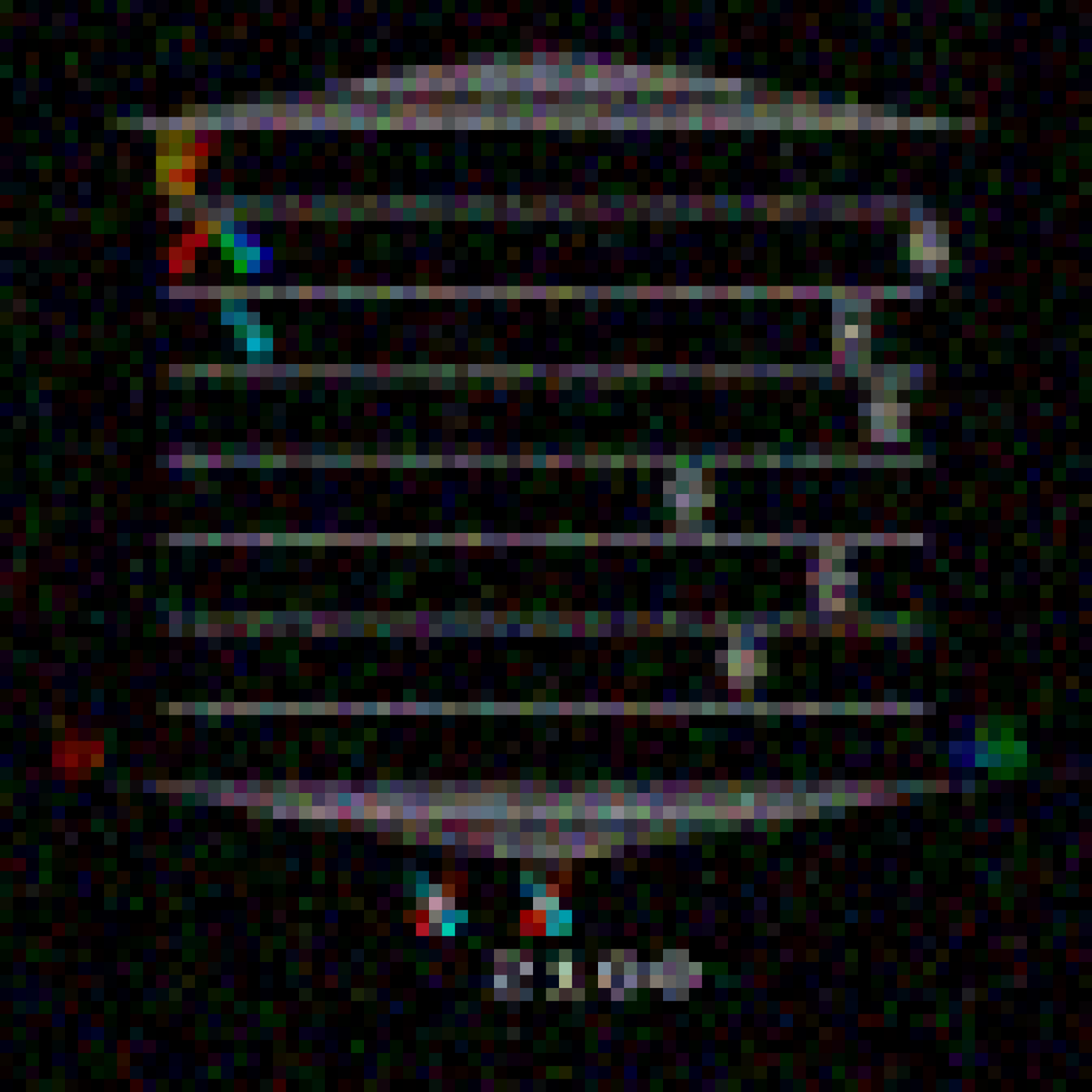
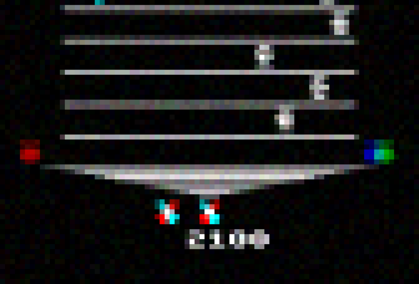
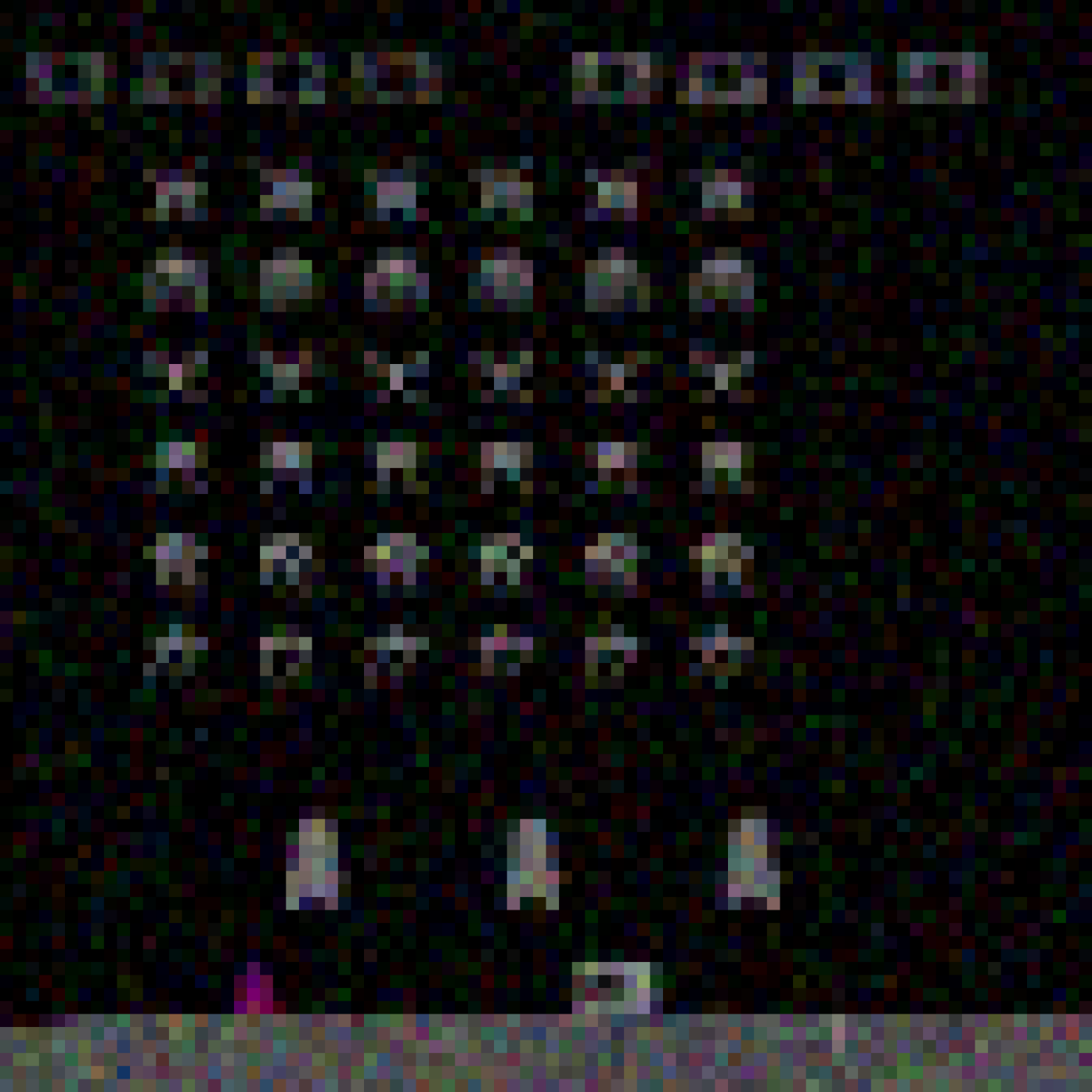
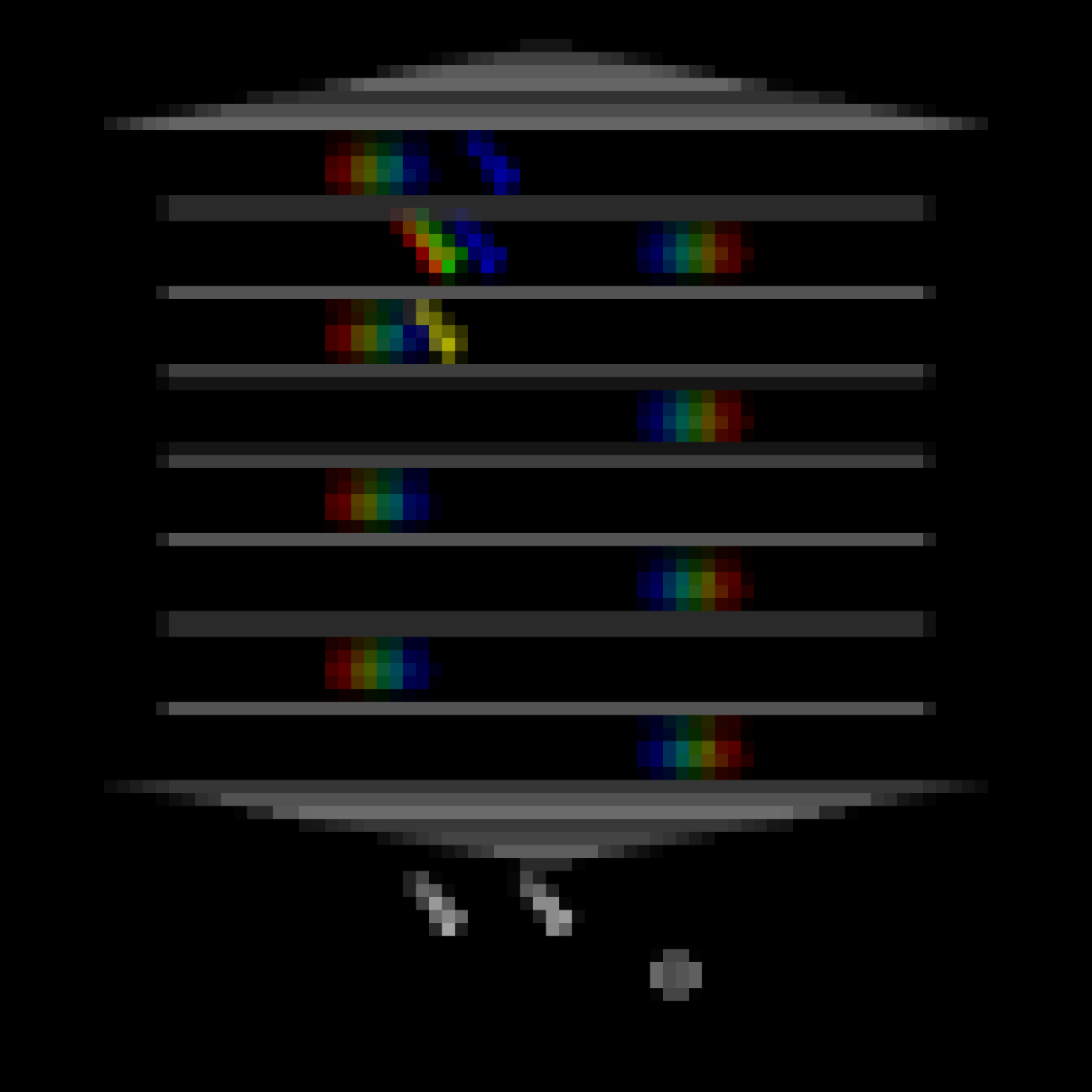
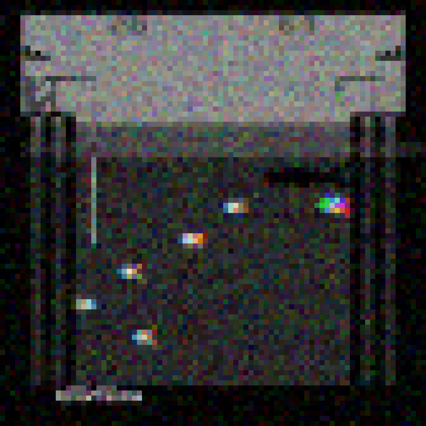
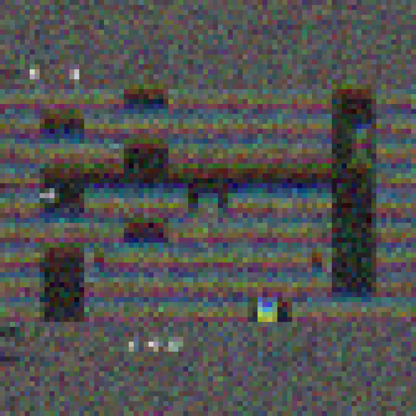
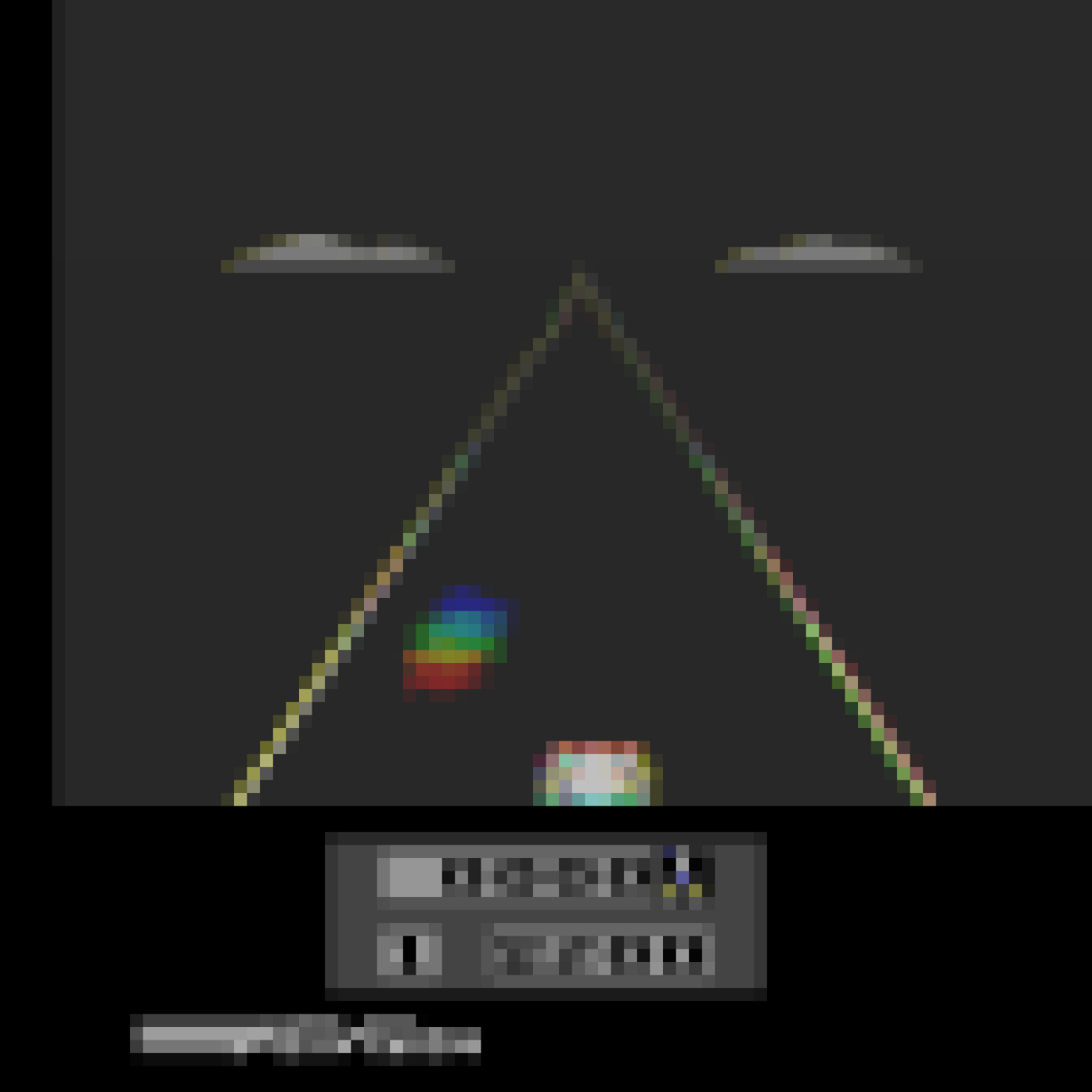
We plot the outlier states on Breakout, Asterix and SpaceInvaders games in Figure 8 and outliers states on Enduro, FishingDerby and Tutankham in Figure 9.














Appendix D Evaluation Phase: Boxplot Results
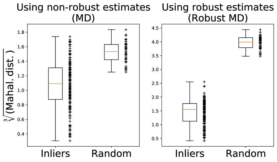
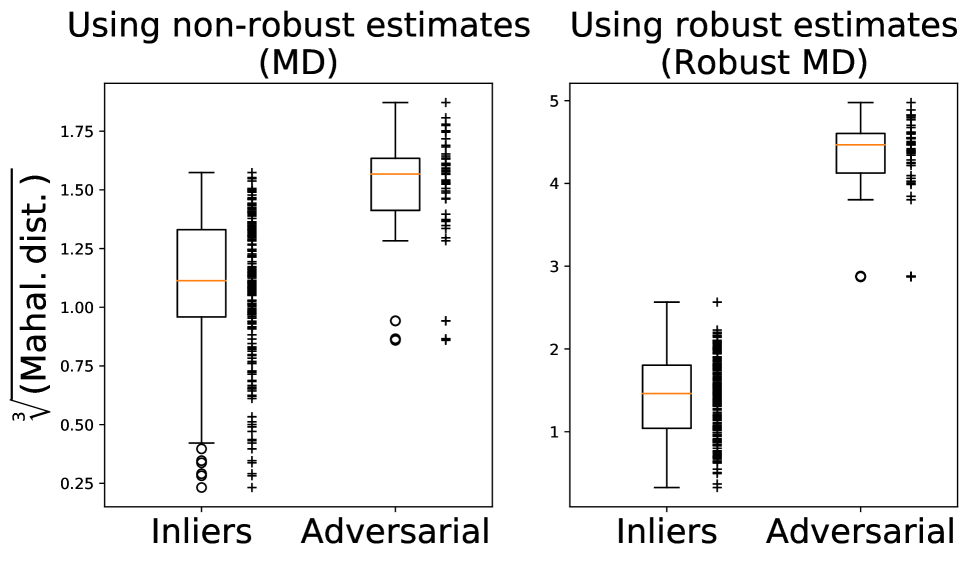
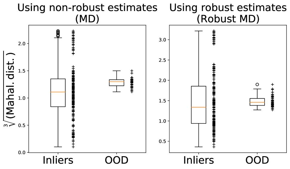
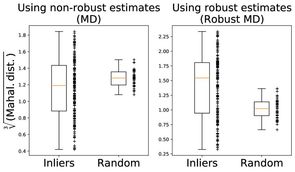
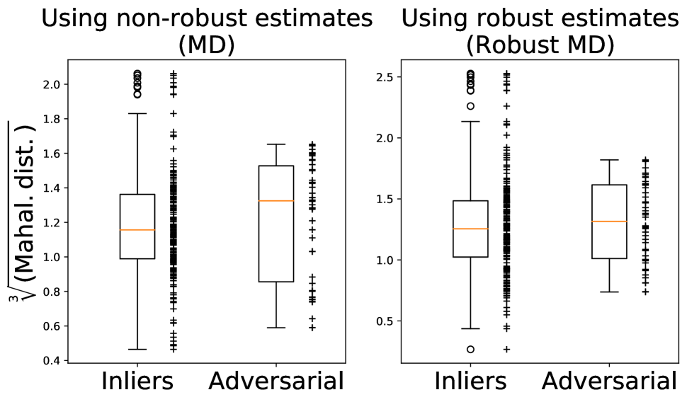
We plot the distributions of inliers and three types of outliers on SpaceInvaders and Asterix games in Figure 10 and 11, respectively. It is worth noting that Robust MD is also capable of enlarging the separation of distributions between inliers and both random and adversarial outliers on SpaceInvaders game, while its benefit seems to be negligible on OOD outliers (Breakout) on SpaceInvaders games as well as in Asterix game. We speculate that it is determined by the game difficulty. Specifically, the PPO algorithm can achieve desirable performance on the simple Breakout game, thus yielding informative feature space vectors. By contrast, there is a room for the generalization of PPO on both SpaceInvaders and Asterix games such that Robust MD might not help while handling the less meaningful state feature vectors on these two games.
Appendix E Evaluation Phase: Sensitivity Analysis
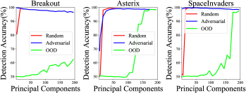
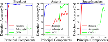
The impact of the number of principal components on the detection performance for robust MD detection in shown in Figure 12. The detection accuracy over all considered outliers tends to improve as the number of principal components increases, except for a slight decline for random and adversarial outliers (red and blue lines) on Breakout game. The increase implies that the subspace spanned by principal components with small explained variance also contains useful information for detecting anomalous states from in-distribution states, which coincides with the conclusion in (Kamoi and Kobayashi 2020). For the result of MD estimation, it is manifested in Figure 13. It turns out that there is still an ascending tendency of detection accuracy as the amount of principal components increases.
Appendix F Training Phase: Setup and More Results
| Hyperparameter | Value |
| Confidence level (1-) | 1-0.05 |
| Moving window size () | 2 |
| Sample size () | 5120 |
| Iteration () | 10000 (1e7 steps in total) |
| Environment number () | 8 |
| Horizon () | 128 |
As a supplement to the results on main pages, we provide the whole results on all six Atari games from Figure 16 to Figure 21. “Mean score” in the first row indicates the accumulated rewards of PPO, “accuracy” and “F1 Score” in the second and third row show the detection performance during RL training. F1 score is computed based on precision and recall. We also find that the cumulative reward is not strongly correlated with detection ability. A high detection accuracy may only improve the cumulative reward to a small degree. It means we may need some other metrics to measure the effect of our detection performance more effectively. Hyperparameters in our methods are shown in Table 4.
Comparing with Single Detector.
We conduct an ablation study of single and double detectors on Breakout games with random and OOD outliers. Figure 14 reveals that compared with single detector, double self-supervised detectors can improve the detection accuracy and thus stabilize the training process. In particular, “MD Double” outperforms “MD Single” significantly, although “Robust MD Single” is comparable to “Robust MD Double”.
Different Proportions of Contamination.
We study different contamination ratios that the agent encounters in the training phase. We train PPO on two, four or six noisy environments among all eight parallel environments with random and OOD outliers. We use PCA to reduce the feature vectors to 50 dimensions, and estimate the detector using Robust MD. Figure 15 shows that the training performance under our robust MD detection. The dashed lines indicate the performance of the Auto baseline. Results show that the training performance of our detection gradually approaches the ideal performance, especially with a higher the contamination ratio.
