Augmenting Depth Estimation with Geospatial Context

Abstract

Modern cameras are equipped with a wide array of sensors that enable recording the geospatial context of an image. Taking advantage of this, we explore depth estimation under the assumption that the camera is geocalibrated, a problem we refer to as geo-enabled depth estimation. Our key insight is that if capture location is known, the corresponding overhead viewpoint offers a valuable resource for understanding the scale of the scene. We propose an end-to-end architecture for depth estimation that uses geospatial context to infer a synthetic ground-level depth map from a co-located overhead image, then fuses it inside of an encoder/decoder style segmentation network. To support evaluation of our methods, we extend a recently released dataset with overhead imagery and corresponding height maps. Results demonstrate that integrating geospatial context significantly reduces error compared to baselines, both at close ranges and when evaluating at much larger distances than existing benchmarks consider.

1 Introduction

Accurately estimating depth is important for applications that seek to interpret the 3D environment, such as augmented reality and autonomous driving. The traditional geometric approach for solving this problem requires multiple views and infers depth by triangulating image correspondences. Lately, more attention has been paid to the single-image variant, which has great potential value but is known to be ill-posed. Ranftl et al. [29] point out that to solve this problem “one must exploit many, sometimes subtle, visual cues, as well as long-range context and prior knowledge.”

One of the primary difficulties with inferring depth from a single image is that there is an inherent scale ambiguity. In other words, different sized objects in the world can have the same projection on the image plane (simply by adjusting the focal length or position in space). Despite this, methods that take advantage of convolution neural networks have shown promise due to their ability to capture prior information about the appearance and shape of objects in the world.

Figure 1: We explore a new problem, geo-enabled depth estimation, in which the geospatial context of a query image is exploited during the depth estimation process.

There are broadly two classes of methods in this space. Supervised approaches assume a ground-truth labeling is provided during training, often obtained from another sensor such as LiDAR. This labeling could be absolute (metric values) or have an unknown scale. Self-supervised approaches, on the other hand, do not require ground-truth depth. Instead, the consistency of multiple inputs (e.g., sequences of images from a video, or a stereo pair) are used to derive depth up to a scaling factor, often by formulating the problem as a novel view synthesis task. For both of these classes of methods, it is common to make strong assumptions about the scale of the scene during training, or to require computation of a scaling factor at inference time in order to interpret the predicted depths.

For example, supervised methods often presume to know the maximum observed depth of the scene, by constraining the output of the network using a sigmoid activation and scaling by the maximum depth [9, 19]. If the scale is unknown, i.e., a scale-invariant loss was used during training, then a scaling factor must be computed at inference to interpret the predictions relative to the world. Such objective functions have been proposed when metric depth is not available or for combining training datasets with different properties. For example, Ranftl et al. [29] align their predictions with the ground-truth via a least squares criterion before computing error metrics. These caveats limit the generalizability of such methods when applying them to real-world imagery from novel locations (e.g., varying depth ranges or lack of ground truth).

A similar phenomena occurs in self-supervised monocular approaches that estimate depth up to an unknown scale. The maximum observed depth of the scene is often used to constrain the predicted depths during training, and a scaling factor is computed at inference to bring the predictions in line with the ground truth. As before, the common strategy in the current literature is to compute this scaling factor using the ground-truth directly (per image), in this case by computing the ratio of the median predicted values and median ground-truth values [12]. The issue of how to calibrate self-supervised monocular depth estimation networks has only recently been highlighted by McCraith et al. [26], who point out that current approaches severely limit practical applications.

Beyond these issues, estimating depth at long ranges is known to be extremely challenging. Zhang et al. [41] note the limitations of LiDAR (sparse, reliable up to 200m) and argue the need for “dense, accurate depth perception beyond the LiDAR range.” Most state-of-the-art depth estimation networks assume a maximum depth of 100 meters for outdoor scenes [12]. Further, popular benchmark datasets for depth estimation are constrained to small ranges, typically below 100 meters (using a depth cap to filter pixels in the ground truth). For example, Ranftl et al. [29] evaluate on four different datasets, ETH3D, KITTI, NYU, and TUM, with the depth caps set to 72, 80, 10, and 10 meters, respectively. Reza et al. [30] have similarly pointed out the need for depth estimation to function at much larger distances.

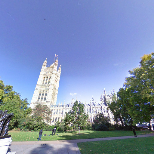
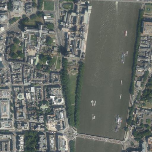
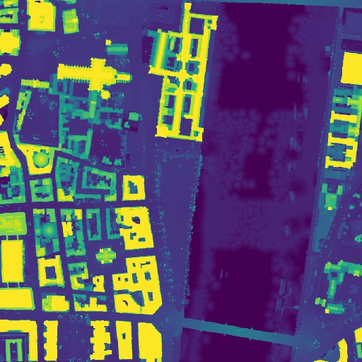
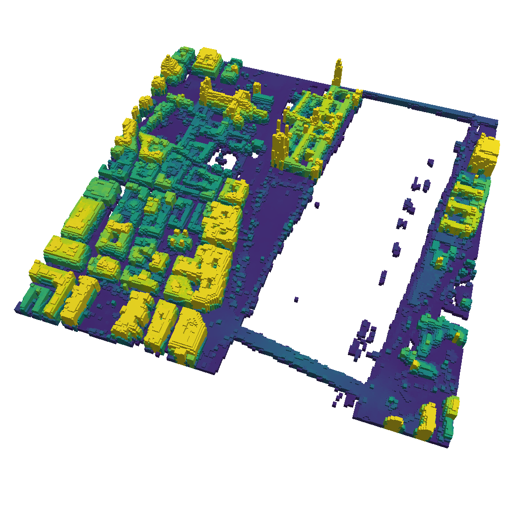
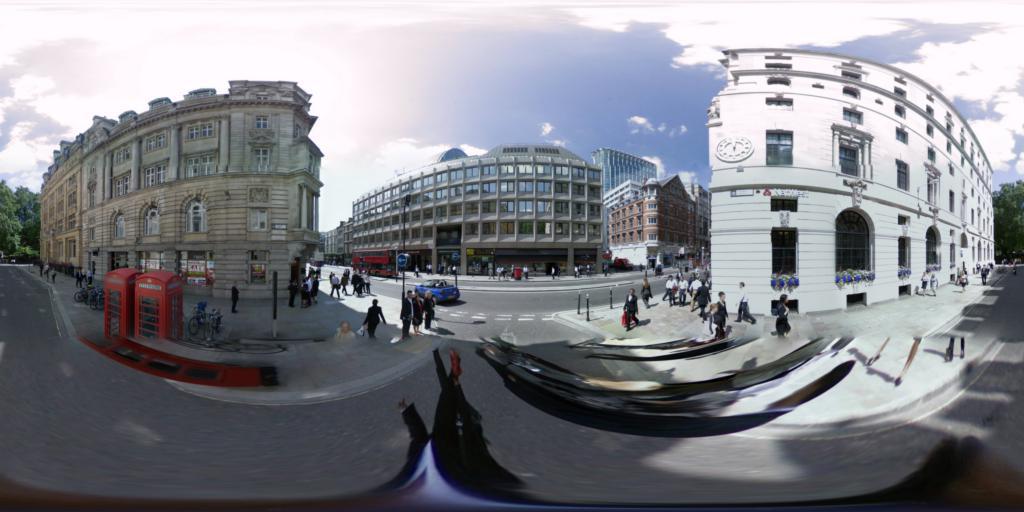
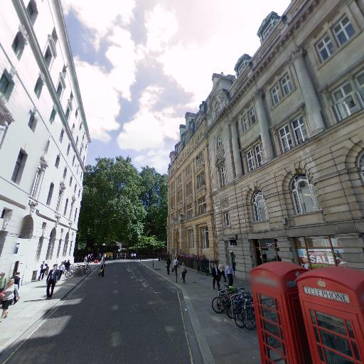
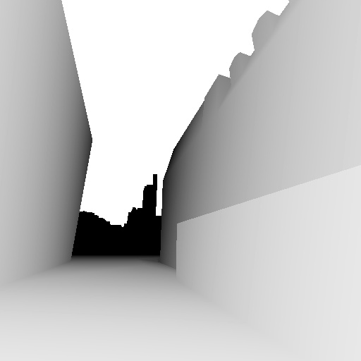
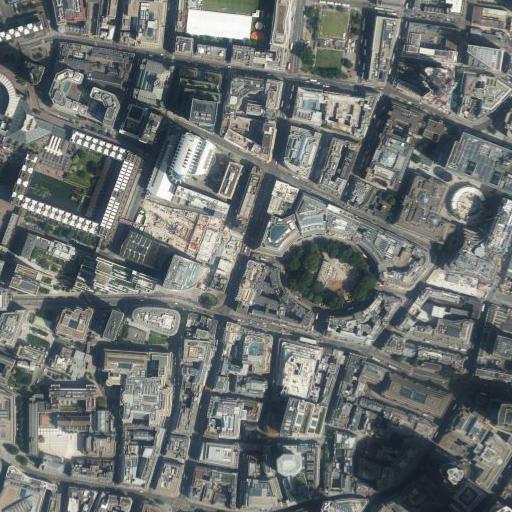
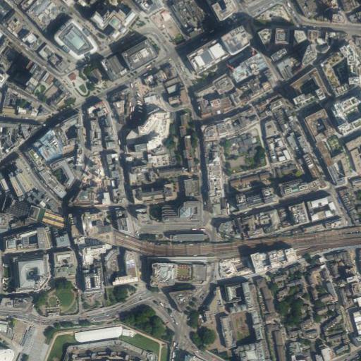
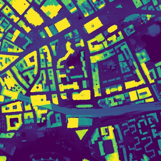
In this work we explore how geospatial context can be used to augment depth estimation, a problem we refer to as geo-enabled depth estimation (Figure 1). Modern cameras are commonly equipped with a suite of sensors for estimating location and orientation. Kok et al. [17] provide an in-depth overview of algorithms for recovering position/orientation from inertial sensors, concluding that as quality has improved and cost has decreased “inertial sensors can be used for even more diverse applications in the future.” Accordingly, a great deal of work has shown that geo-orientation information is extremely valuable for augmenting traditional vision tasks [24, 35, 25, 40, 39].

Given a geocalibrated camera, we explore how to inject geospatial context into the depth estimation process. In this scenario, our goal is to develop a method that takes advantage of the known geocalibration of the camera to address the previously outlined weaknesses. Specifically, we want to use geospatial context to 1) reduce the inherent scale ambiguity and to 2) enable more accurate depth estimation at large distances. Our key insight is that if the location of the capturing device is known, the corresponding overhead viewpoint is a valuable resource for characterizing scale.

We propose an end-to-end architecture for depth estimation that uses geospatial context to infer an intermediate representation of the scale of the scene. To do this, we estimate a height (elevation) map centered at the query image and transform it to a synthetic ground-level depth map in a differentiable manner via a sequence of voxelization and ray casting operations. This intermediate representation is metric, and we fuse it inside of an encoder/decoder segmentation architecture that outputs absolute depth estimates. Importantly, our approach makes no assumptions during training about the maximum observed depth and requires no post-processing step to align predictions.

To support evaluating our methods, we extend the recently released HoliCity dataset [44] to include overhead imagery and corresponding height data from a composite digital surface model. Extensive experiments show that when geospatial context is available our approach significantly reduces error compared to baselines, including when evaluating at much longer depth ranges than considered by previous work.

Figure 2: We introduce the HoliCity-Overhead dataset which extends the recently introduced HoliCity dataset [44] to include overhead imagery and associated ground-truth height maps. From left to right, equirectangular panorama, perspective cutout, corresponding depth map, co-located overhead image, and corresponding height map.

2 Related Work

Traditional work in depth estimation relied on geometric cues from multiple images to infer depth. Interest quickly shifted to the single-image variant of the problem with early approaches relying on a set of assumptions about the geometric layout of the scene [14]. For example, Delage et al. [5] proposed a 3D reconstruction method for a single indoor image that makes assumptions about the relationship between vertical and horizontal surfaces and uses visual cues to find the most probable floor-wall boundary. Saxena et al. [34] later assumed the environment is made up of many small planes and estimated the position and orientation of each using a Markov random field.

More recently in machine vision it has become common to directly regress depth using convolutional neural networks. Supervised approaches use ground-truth depth from RGB-D cameras, LiDAR sensors, or stereo matching [7]. In this space there has been much exploration into various architecture and design choices [18, 9, 1, 19, 20]. However, the primary challenge for supervised methods remains the difficulty in acquiring high quality and varied training data. To navigate this issue, Atapour-Abarghouei and Breckon [2] propose to train using a synthetic dataset and then apply style transfer to improve performance on real-world images. Other work has relaxed the requirement for absolute depth supervision by proposing scale-invariant objective functions [4]. Ranftl et al. [29] argue that performance is primarily impacted by the lack of large-scale ground truth, proposing a scale-invariant loss that enables mixing of data sources.

Alternatively, self-supervised methods circumvent the need for ground-truth depth entirely, instead relying on multiple inputs (e.g., sequences of images from a video, or a stereo pair) during training to derive depth up to a scaling factor. The problem is commonly reformulated as an image reconstruction task with [11] or without [43, 12, 42] known camera pose information. While self-supervised methods that take advantage of stereo supervision can infer scale directly from the known camera baseline [12], self-supervised monocular approaches suffer from the need to align predictions with the ground-truth at inference by computing the scaling factor [26]. When considering both supervised and self-supervised approaches, it is common to make an assumption about the maximum observed depth during training [9, 19]. In addition, popular benchmarks such as ETH3D and KITTI are evaluated sub-100 meters. This limits the practical application of these methods when considering images from novel locations, thus methods that function at larger distances are needed [30].

Motivated primarily by the surge in interest in autonomous driving, another strategy is to frame the problem as depth completion or depth refinement where, in addition to the input image, an approximate (possibly sparse) depth image is provided (e.g., from a LiDAR sensor). Here, the objective is to produce a dense, more accurate depth map [31]. Our approach is similar to this line of work in the sense that we use geospatial context to produce an intermediate depth estimate that is used along with the input image to infer a final depth prediction. Though we focus on integrating geospatial context, our method can conceivably be combined with any recent depth refinement approach.

Geospatial context has become a powerful tool for improving the performance of traditional vision tasks. For example, Tang et al. [35] consider the task of image classification and show how geolocation can be used to incorporate several different geographic features, ultimately improving classification performance. Similarly, overhead imagery has proven to be useful as a complementary viewpoint of the scene. Luo et al. [24] combine hand-crafted features for a pair of ground-level and overhead images to improve ground-level activity recognition. In the realm of image geolocalization, overhead imagery has been used as an alternative to a ground-level reference database [21, 38] to enable dense coverage. Other use cases include making maps of objects [25, 36] and visual attributes [39, 32], understanding traffic patterns [37], detecting change [10], and visualizing soundscapes [33]. To our knowledge, this work is the first to consider how geospatial context can be used to improve depth estimation.

Figure 3: An overview of our approach. Given a geolocated image, we transform a co-located height map to an intermediate representation of the scale of the scene via a series of differentiable operations that take advantage of the known camera geocalibration. We then fuse it into an encoder/decoder segmentation architecture that operates on the ground-level image. Importantly, our approach can function on a known height map if available (e.g., from a composite DSM), or instead estimate height from a co-located overhead image (shaded region).

3 HoliCity-Overhead Dataset

To support our experiments, we introduce the HoliCity-Overhead dataset which extends the recently introduced HoliCity [44] dataset. HoliCity is a city-scale dataset for learning holistic 3D structures such as planes, surface normals, depth maps, and vanishing points. The dataset was constructed by taking advantage of a proprietary computer-aided design (CAD) model of downtown London, United Kingdom with an area of more than $20km^{2}$. Note that as labels are derived from the CAD model, they do not contain dynamic objects (e.g., pedestrians). We do not consider this a limitation as deriving depth in this manner enables ground-truth depth values at significantly greater ranges compared to existing datasets (on the order of kilometers for HoliCity), which is crucial for supporting our goal of enabling more accurate depth estimation at larger distances.

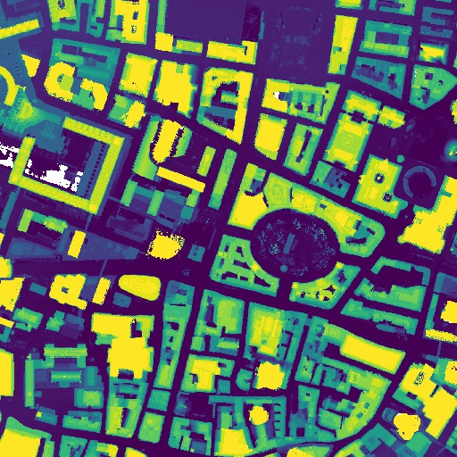
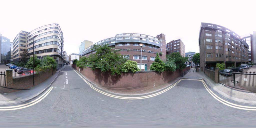
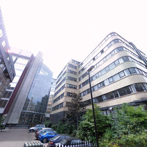
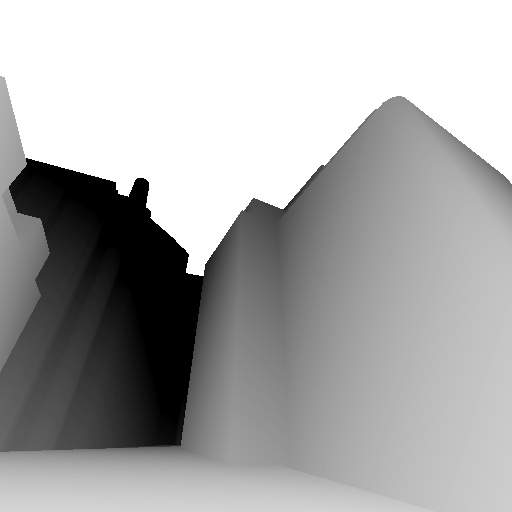
In the source region, 6,300 panoramas were collected from Google Street View with a native resolution of $6,656\times 13,312$. The individual panoramas were aligned with the CAD model such that the average median reprojection error is less than half a degree. From each panorama, eight perspective cutouts (of size $512\times 512$) were extracted at 45 degrees apart, with yaw and pitch angles randomly sampled and field-of-view set to $90^{\circ}$. Labels were generated for each cutout using the CAD model. Importantly, the geo-orientation information for the original $360^{\circ}$ equirectangular panoramas, as well as the camera parameters defining the perspective cutouts, are provided. Example images from the dataset are shown in Figure 2.

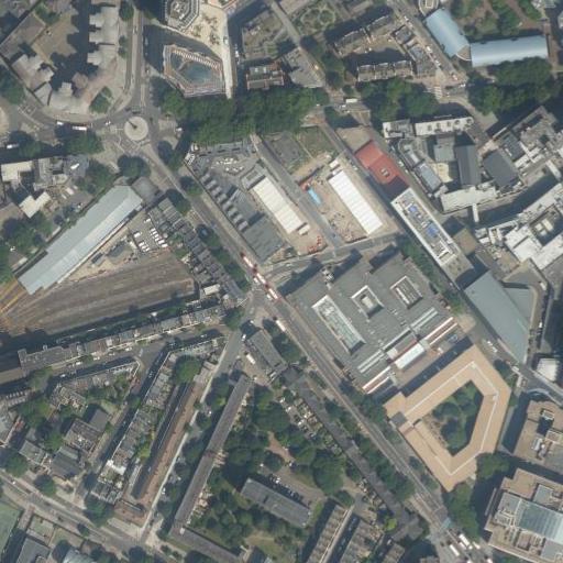
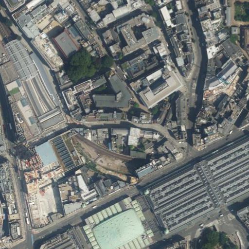
For our purposes, we extended the dataset to include overhead imagery and ground-truth height maps, which we refer to as the HoliCity-Overhead dataset. For each Google Street View panorama, we collected a co-located overhead image at multiple resolutions (zoom levels 16-18) from Bing Maps (each of size $512\times 512$). Then, we generated a height map for each overhead image by aligning to a 1 meter composite digital surface model (DSM) of London produced by the Environment Agency in 2017. The DSM data is made publicly available via the UK government at the open data portal. Examples of the resulting overhead image and height map pairs contained in the HoliCity-Overhead dataset are shown in Figure 2 (right).

Though HoliCity provides an official evaluation split, ground-truth data for the test set is reserved for a future held-out benchmark. As such, in our experiments we report performance numbers using the validation set and instead reserve a small portion of the training set for validation.

4 Geo-Enabled Depth Estimation

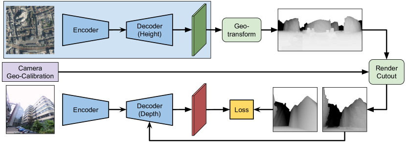
We propose an end-to-end architecture for depth estimation that integrates geospatial context. Figure 3 provides a visual overview of our approach. For the purposes of description, we outline our approach as if a height map is estimated from a co-located overhead image, but it can be provided directly as input if available.

4.1 Approach Overview

Given a geocalibrated ground-level image (i.e., known geolocation, orientation, field of view), our approach has two primary components. First, we estimate a height map from a co-located overhead image and use it to generate an intermediate representation of the scale of the scene. To generate the intermediate representation from the height map, we render a synthetic ground-level depth image through a sequence of differentiable operations that take advantage of the known camera geocalibration (i.e., conversion to a voxel representation and ray casting). This intermediate representation is metric and has many potential uses. The second component of our approach performs joint inference on a ground-level image and the synthetic depth image in an encoder/decoder style segmentation architecture, fusing the two modalities inside the decoder.

4.2 Inferring Scale from an Overhead Viewpoint

We leverage geospatial context to generate an intermediate representation of the scale of the scene from an overhead viewpoint.

4.2.1 Estimating a Height Map

Given a geocalibrated ground-level image and a co-located overhead image, we first estimate a per-pixel height map from the overhead image. We represent this as a supervised regression task that outputs per-pixel metric height values. For our segmentation architecture, we use LinkNet [3] with a ResNet-34 [13] encoder (initialized using weights from a model trained on ImageNet [6]). For the objective function, we minimize the Pseudo-Huber loss (also recognized as the Charbonnier loss):

$$\mathcal{L}_{height}=\delta^{2}(\sqrt{1+((y-\hat{y})/\delta)^{2}}-1),$$ (1)

where $y$ and $\hat{y}$ are the observed and predicted values, respectively. The Pseudo-Huber loss is a smooth approximation of the Huber loss, where $\delta$ controls the steepness.

4.2.2 Synthesizing a Depth Panorama

Figure 4: Transforming a height map from an overhead viewpoint to a depth panorama using a voxel representation combined with ray casting. (left, bottom) The input height map and (right, bottom) the generated depth panorama. As the ground sample distance of the overhead height map is known, the resulting depth panorama is metric.

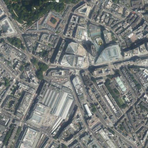
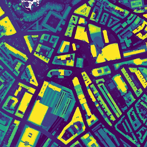
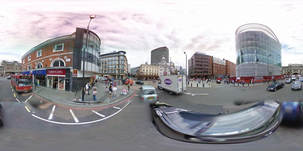
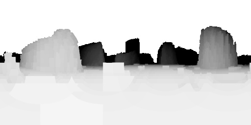
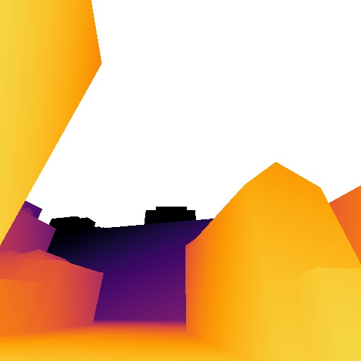
Drawing inspiration from Lu et al. [23] who tackle the problem of cross-view image synthesis, we use the estimated height map to render north aligned panoramic depth images. Given that the overhead imagery has known ground sample distance (the spatial extent of each pixel in the world is known), we use the overhead height map to construct a voxel occupancy grid. The grid is generated such that voxel $v_{i,j,k}=1$ if height value $h_{i,j}>k$ at pixel location $(i,j)$. The overhead image, and subsequently the voxel grid, is centered at the geolocation of the query ground-level image. Then, a synthetic panoramic depth image is constructed from the voxel grid by sampling at uniform distances along the ray for each pixel in the output panorama. The output depth is set to the minimum sampling distance that intersects a non-zero voxel. Figure 4 visualizes the output of this process using a ground-truth height map.

4.2.3 Extracting a Perspective Cutout

The previous step generates a synthetic ground-level panoramic depth image directly from an overhead height map. For use in our end-to-end system, we also implement a differentiable layer for extracting perspective cutouts from a 360^∘ panorama. Given an equirectangular panorama and target geocalibration (yaw, pitch, roll, field of view), we extract the corresponding perspective image by treating the panorama as a cylindrical image and sampling the projections onto the image plane under the given camera geometry. We implement this as a separate layer so that the panoramic depth image can be accessed directly, and additionally for resource conservation in the event that several perspective cutouts are needed from a single panorama.

4.3 Depth Refinement using Geospatial Context

Table 1: HoliCity evaluation results (depth cap 80m).

	Abs Rel	Sq Rel	RMSE	RMSE log	$\delta<1.25$	$\delta<1.25^{2}$	$\delta<1.25^{3}$
overhead	0.886	21.564	10.571	0.602	0.314	0.600	0.771
ground (variant of [1])	0.503	10.631	5.626	0.301	0.675	0.876	0.940
ours (concatenate)	0.515	14.790	5.057	0.290	0.711	0.883	0.944
ours	0.501	12.205	4.895	0.279	0.711	0.893	0.950
ground + median scaling (overhead)	0.923	25.355	8.635	0.457	0.400	0.709	0.847
ground + median scaling (ground truth)	0.229	3.249	5.388	0.255	0.749	0.905	0.957
ours + median scaling (ground truth)	0.216	2.967	4.782	0.239	0.774	0.920	0.964

Here we outline our depth refinement architecture (Figure 3, bottom) that takes as input a ground-level image and the intermediate estimate of scale generated from a co-located height map. We start from the architecture proposed by Alhashim and Wonka [1] and regress depth using an encoder/decoder segmentation network with skip connections. In this approach, the decoder consists of a series of upsampling blocks. In each block, the input feature map is upsampled via bilinear interpolation, concatenated with the corresponding feature map from the encoder (skip connection), and passed through two $3\times 3$ convolutional layers with the number of output filters set to half of the input filters. Unlike existing work, which often estimates half resolution depth, we add an extra convolutional transpose layer before the final output layer of the decoder in order to generate full resolution depth. For the encoder, we use DenseNet-161 [15] pretrained on ImageNet.

To incorporate geospatial context (in the form of a synthetic depth image obtained from the estimated height map) we fuse it with image features inside the decoder. Specifically, before each convolutional layer and upsampling block, we concatenate the synthetic depth image as an additional channel of the input feature map, resizing as necessary. The final two layers of the decoder (convolutional transpose layer and output convolutional layer) are excluded from this process. Fusing in the decoder allows the encoder to learn features solely focusing on the content of the query image.

Similar to height estimation, we minimize the Pseudo-Huber Loss (1). However, we omit pixels from the objective function that do not have ground-truth depths using a validation mask. The final loss becomes

$$\mathcal{L}=\alpha_{h}\mathcal{L}_{height}+\mathcal{L}_{depth},$$ (2)

where $\alpha_{h}$ is a weighting term used to balance the two tasks. Our approach can be thought of as a depth refinement technique that takes into account the overhead approximation of scene scale.

4.4 Implementation Details

We implement our methods using PyTorch [28] and PyTorch Lightning [8]. Our networks are optimized using Adam [16] with the initial learning rate set to $1e^{-4}$. All networks are trained for 25 epochs and the learning rate policy is set to reduce-on-plateau by an order of magnitude using the validation set (patience equal to 5 epochs). For the Pseudo-Huber loss, we set $\delta=2$. To balance the two tasks, we set $\alpha_{h}=0.1$. This weighting term is decreased a single time after 5 epochs, by a factor of 10. When estimating heights, we normalize each ground-truth height map individually such that the minimum value is zero. For rendering perspective cutouts, we set non-intersections to a value of -1.

5 Evaluation

We evaluate our methods quantitatively and qualitatively through a variety of experiments. Results demonstrate that our approach, which builds on a recent state-of-the-art method to inject geospatial context, significantly reduces error at close ranges while simultaneously enabling more accurate depth estimates at larger ranges than have been previously considered.

Baseline Methods

To evaluate the proposed architecture, we compare against several baseline methods that share low-level components with our proposed method. Our full approach is outlined in Section 4 and is subsequently referred to as ours. We also compare against a baseline that omits geospatial context from our approach (referred to as ground). Note that without geospatial context, this baseline is simply a variant of the recent state-of-the-art method of Alhashim and Wonka [1]. Additionally, we compare against a baseline that uses only the intermediate estimate of scale, derived from geospatial context, as the final prediction (referred to as overhead). Finally, we compare against a baseline that concatenates the intermediate estimate as an additional channel to the input image and we refer to this as ours (concatenate). The strategy for this baseline is similar in concept to the recent work of Liu and Li [22] who add orientation as an additional input channel for cross-view image geolocalization.

5.1 Ablation Study

We present results using the HoliCity-Overhead dataset. As mentioned previously, we report metrics on the HoliCity [44] validation set as ground-truth data for the test set is unavailable. Unless otherwise specified, all methods are trained using HoliCity-Overhead data corresponding to zoom level 17 (approx. 0.74 meters per pixel, or 190 meter half width) and use the known height map.

Table 2: Estimated versus known height maps (HoliCity, depth cap 80m).

	RMSE	RMSE log
ours (estimated height)	4.935	0.287
ours (known height)	4.895	0.279

For our initial experiment, we evaluate the ability of our approach at short ranges (depth cap of 80 meters), computing metrics as in [12]. Table 1 summarizes the results of this study. As expected, the ground-only baseline outperforms the overhead-only baseline, likely due to the difficulty in precisely recovering fine-grained details from an overhead viewpoint. Despite the limited evaluation range, our methods that integrate geospatial context significantly outperform all baselines, e.g., by over half a meter in RMSE versus the ground-only baseline. Additionally, our approach of fusing in the decoder outperforms the variant of our method that concatenates as an additional input channel.

In addition, we show the impact of adding median scaling (a per-image scaling factor used to align results) to the ground-only baseline using both the overhead estimate and the ground truth. This result demonstrates the benefit of our end-to-end architecture over an approach that simply uses the intermediate estimate of scale directly as a calibration tool. Though we have previously noted the impracticality of median scaling using the ground truth, for fairness we show that our approach can similarly benefit, achieving significantly lower error.

Finally, Table 2 shows that our method that simultaneously learns height maps (from co-located overhead images) performs competitively against our approach that accepts known height maps directly (e.g., from a composite DSM). These results show that geospatial context, if available, can be extremely useful for augmenting depth estimation, even at small ranges.

5.2 Long Range Depth Estimation

Next, we analyze the performance of our methods at much greater distances. One of the major limitations of existing work is that evaluation is typically limited to less than 100 meters [29, 30]. This can be partly attributed to the increased difficulty of accurately estimating depth at long ranges, but also due to the limited range of LiDAR sensors, which are often used for collecting ground truth. An advantage of the HoliCity dataset [44] is that the truth labels are derived from a CAD model, enabling ground-truth depth to reflect much larger distances.

Figure 5: Integrating geospatial context reduces average error as distance increases when compared to baselines, including an overhead-only approach.

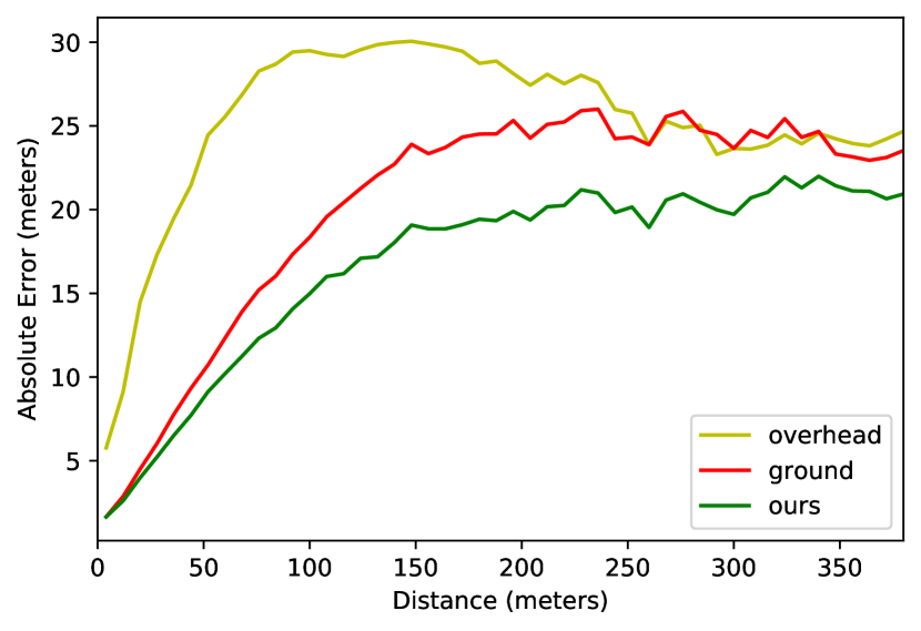
Figure 5 visualizes the performance of our approach over a range of up to 400 meters, using absolute error as the metric, versus two baselines. As expected, average error increases as the magnitude of the depth increases. Our method not only exhibits lower depth error overall, but greatly reduces error at long ranges. We attribute this to our explicit intermediate representation of scale derived from an overhead viewpoint, which enables a good approximation of depth even at far distances.

Figure 6: Evaluating the impact of varying ground sample distance. As anticipated, the greater spatial coverage of lower zoom levels positively impacts depth estimation performance at greater distances.

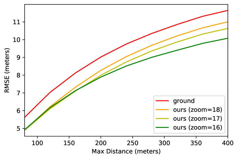
Finally, we evaluate the impact of varying ground sample distance on our methods. In other words, does having a greater spatial coverage in the overhead height map positively impact depth estimation performance? Intuitively this makes sense, as greater spatial coverage in the height maps would enable capturing objects further away in the synthetic depth panorama (Figure 4) and subsequent perspective cutout, with the trade-off of less detail (i.e., being zoomed out). For this experiment, we train variants of our method for the different zoom levels of imagery contained in HoliCity-Overhead. Figure 6 visualizes the results, with the x-axis representing the maximum depth considered (depth cap) when computing the error metric (RMSE). As anticipated, at further distances, starting from height maps with greater spatial coverage leads to an advantage, with all methods significantly outperforming the ground-only baseline.

5.3 Impact of Geo-Orientation Accuracy

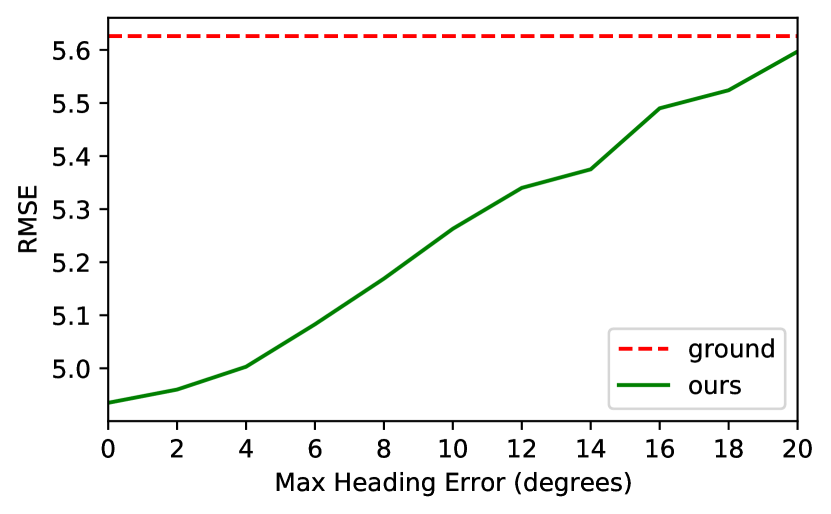
As our approach relies on geospatial context, we explore the ability of our method to handle increasing levels of error in geo-orientation. Note that as the HoliCity [44] dataset has non-zero alignment error, previous results already demonstrate this to a degree. Since high-end systems can achieve position accuracy on the order of centimeters [27], we assume accurate geolocation and focus our attention on orientation. Specifically, we follow the findings of Kok et al. [17] who demonstrate that it is generally easier to obtain accurate roll and pitch estimates from inertial sensors than it is to obtain accurate heading (yaw) estimates. We evaluate our approach by adding increasing levels of maximum heading error, $\theta$, at inference, by sampling uniformly on the interval $[-\theta,\theta]$. Note that the average error in this scenario is approximately $\frac{\theta}{2}$. Intuitively, performance should decrease as orientation error increases. Figure 7 shows the results of this experiment. Our approach still outperforms the ground-only baseline even with significant added noise. Additionally, in the supplemental material we demonstrate how components of our approach can be used to refine geo-orientation.

Figure 7: Evaluating performance with increasing orientation error. Even with significant noise, our approach outperforms the ground-only baseline.

5.4 Application: Calibrating Self-Supervised Monocular Approaches

In this section, we demonstrate the potential of our method to be used as a tool for calibrating self-supervised depth estimation approaches. As discussed previously, self-supervised monocular methods can only estimate depth up to an unknown scale and a scaling factor must be computed to align predictions. Recent work has highlighted that using the ground-truth to compute this scaling factor is not a practical solution [26]. We begin by investigating the impact this scaling step has on performance by analyzing a recent state-of-the-art self-supervised approach, Monodepth2 [12], using the KITTI depth benchmark.

Though Monodepth2 only predicts depth up to an unknown scale, depth predictions are constrained to a range of [0, 100] meters (for KITTI) by passing the final logits through a sigmoid activation and scaling by a fixed max depth value. To align predictions, median scaling is used, where the scaling factor for each image is computed from the ratio of the median predicted values and median ground-truth values (considering only pixels inside the depth cap). Table 3 shows results for Monodepth2 with and without median scaling. For this experiment, the depth cap is set to 80m as is typical for KITTI. To generate these results, we use a pretrained model and evaluation scripts made available by the authors. As observed, median scaling has a drastic impact on performance, with the average root-mean-square error (meters) increasing by almost a factor of four when it is disabled.

Next, we evaluate the ability of our approach to be used as a calibration tool. For this experiment, we use the HoliCity-Overhead dataset as overhead imagery and height data are not available for KITTI. Note that retraining Monodepth2 on HoliCity is not possible due to the lack of image sequences. Using the same process outlined above and the same pretrained model, we replace the ground-truth depth values in median scaling with our intermediate representation of scale. Table 4 shows results for three different scenarios: with median scaling disabled, median scaling using the ground truth, and median scaling using the depth from the voxelized overhead height map as in our approach. As observed, when ground-truth is not available our approach drastically improves results compared to no scaling.

Table 3: Evaluating Monodepth2 [12] on KITTI.

	RMSE	RMSE log
no scaling	19.176	3.459
median scaling (ground truth)	4.863	0.193

Table 4: Evaluating Monodepth2 [12] on HoliCity.

	RMSE	RMSE log
no scaling	17.555	3.054
median scaling (overhead)	15.743	1.138
median scaling (ground truth)	14.105	1.064

6 Conclusion

We explored a new problem, geo-enabled depth estimation, in which the geospatial context of a query image is leveraged to improve depth estimation. Our key insight was that overhead imagery can serve as a valuable source of information about the scale of the scene. Taking advantage of this, we proposed an end-to-end architecture that integrates geospatial context by first generating an intermediate representation of the scale of the scene from an estimated (or known) height map and then fusing it inside of a segmentation architecture that operates on a ground-level image. An extensive evaluation shows that our method significantly reduces error compared to baselines, especially when considering much greater distances than existing evaluation benchmarks. Ultimately our hope is that this work demonstrates that existing depth estimation techniques can benefit when geospatial context is available.

Supplemental Material :
Augmenting Depth Estimation with Geospatial Context

This document contains additional details and experiments related to our methods.

1 HoliCity-Overhead Dataset

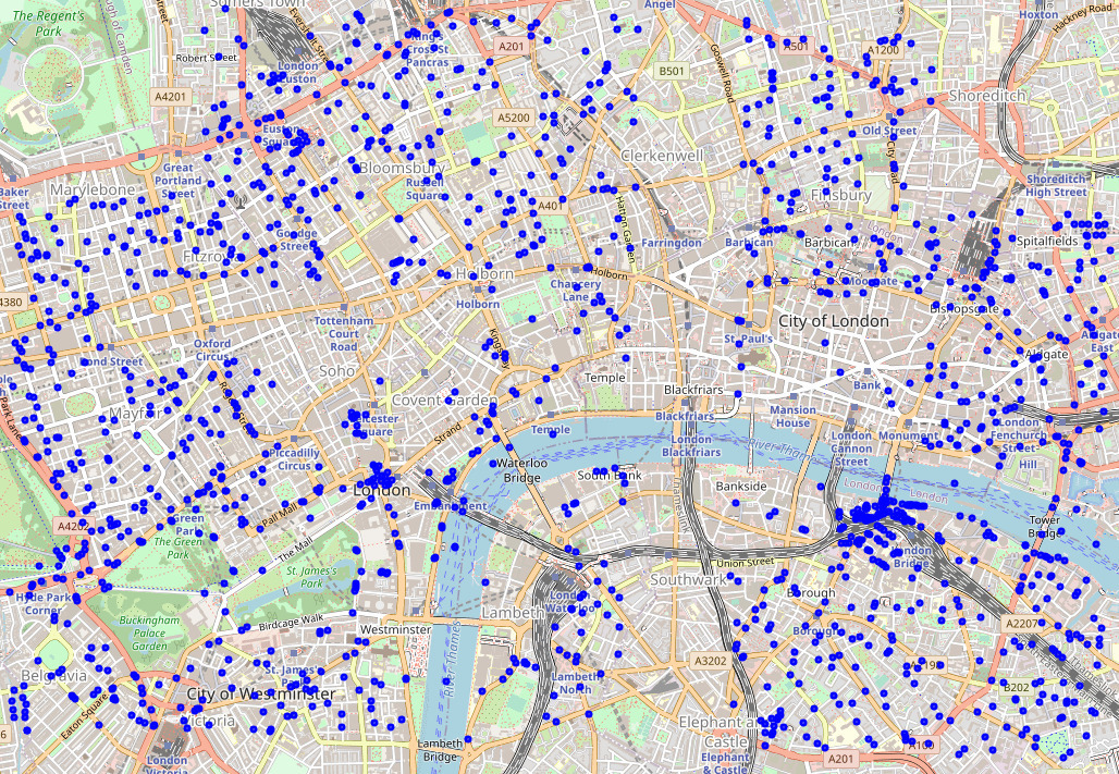
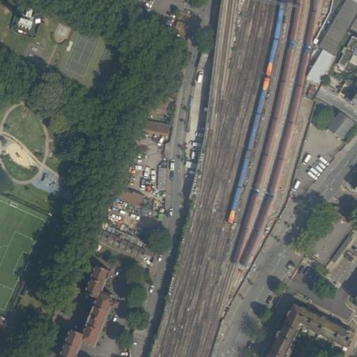
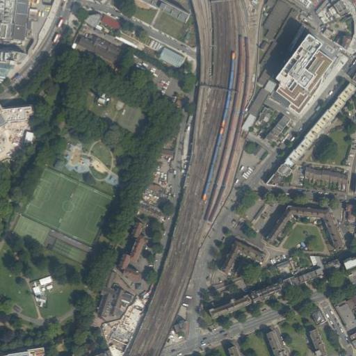
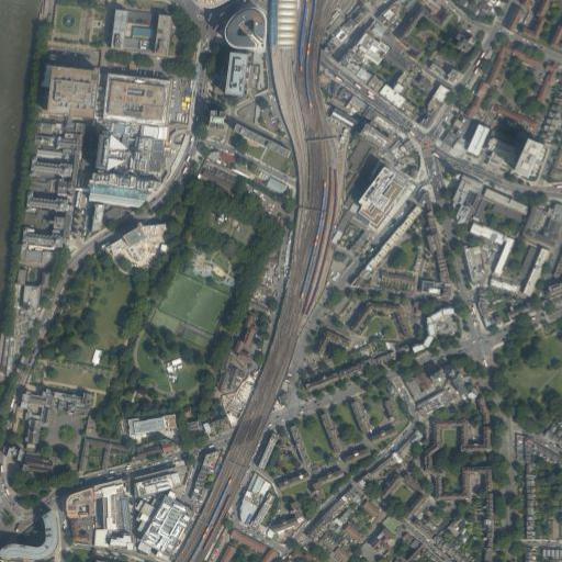
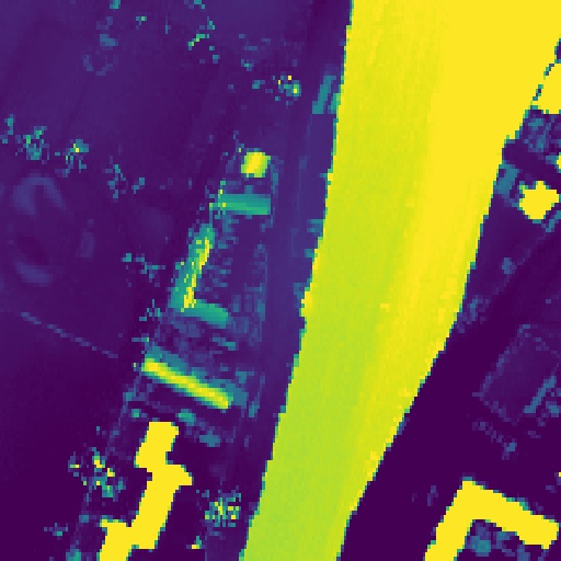
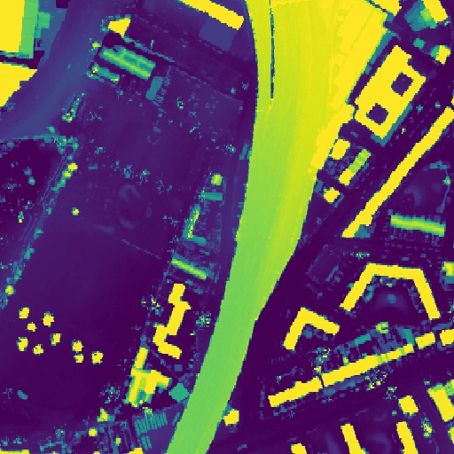
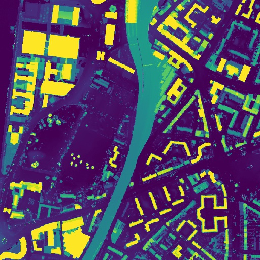
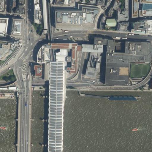
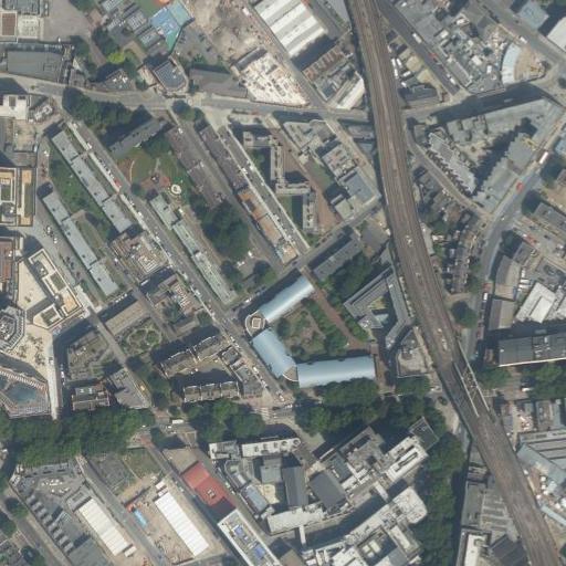
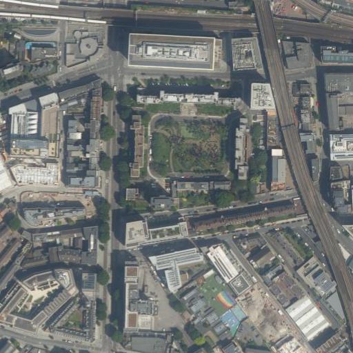
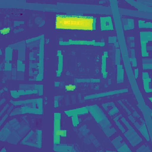
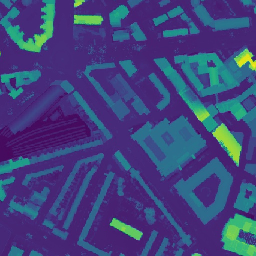
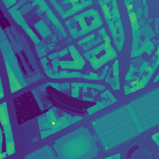
We introduced the HoliCity-Overhead dataset, an extension of the the HoliCity [44] dataset that includes overhead imagery and height data. Figure S1 visualizes the coverage of the original dataset in downtown London, UK. Figure S2 shows example overhead images and aligned height map pairs (each image of size $512\times 512$) at the different zoom levels we collected (i.e., varying ground sample distance or ground resolution).

2 Extended Results

We present additional evaluation of our methods using the HoliCity-Overhead dataset.

2.1 Height Estimation

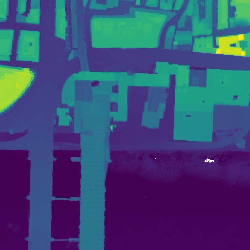
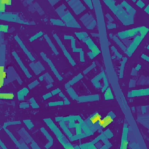
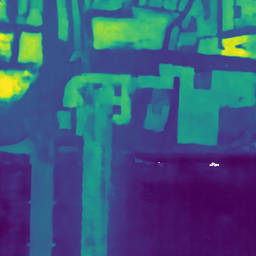
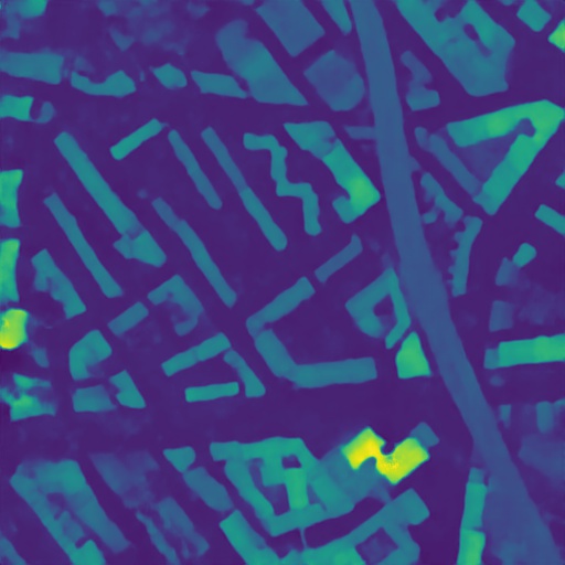
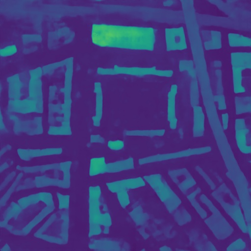
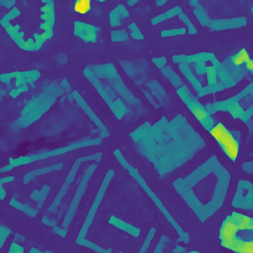
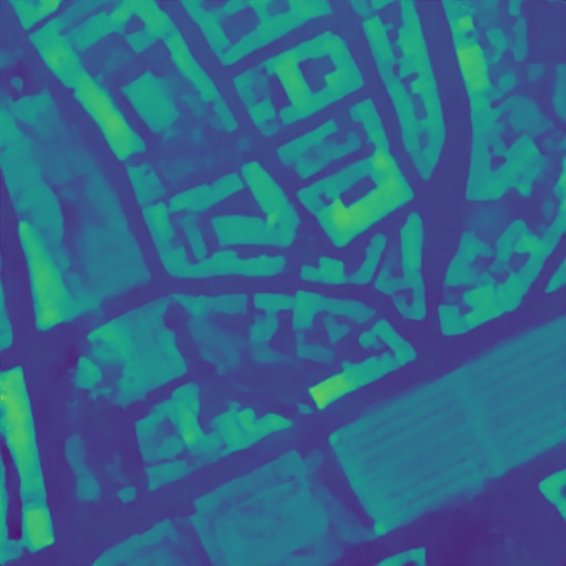
Table S1 shows results for height estimation, generated using our method (Section 4 of the main paper). For this experiment we used the zoom level 17 imagery, which equates to a ground sample distance of approximately .74 meters per pixel over London. Though height estimation is only an intermediate task of our network and not the primary objective, our approach achieves good performance in several metrics. Figure S3 shows example height maps generated using our approach alongside the ground truth, with yellow indicating larger values.

Figure S1: Visualizing the coverage of the HoliCity [44] dataset. The locations of the ground-level panoramas are shown as blue dots (subsampled).

zoom 18	zoom 17	zoom 16

Figure S2: Example data from the HoliCity-Overhead dataset at different zoom levels (i.e., varying ground sample distance). (top) Overhead image and (bottom) height map from composite digital surface model.

Table S1: Height estimation results on HoliCity-Overhead.

	MAE	RMSE	RMSE log
ours (height est.)	3.333	5.225	0.470

image
label
prediction

Figure S3: Example height maps generated by our approach where yellow represents larger values.

2.2 Scale Factor Analysis

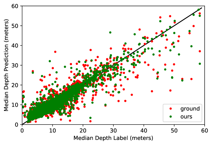
Though our method requires no computation of a scaling factor at inference, we can analyze the performance of our method in terms of scale. Figure S4 shows a scatter plot (per image) where the x-axis is median depth from ground-truth and the y-axis is median depth from prediction. Note that in median scaling, the scaling factor is estimated as the ratio of these two quantities. For this visualization, points closer to the diagonal indicate better alignment in scale. As observed, our approach is generally closer to the diagonal when compared against the ground-only baseline.

Figure S4: Visualizing median depth of ground-truth versus median depth of prediction (the ratio of which is the scale factor for median scaling) for our method versus a baseline. Each dot corresponds to an image in the HoliCity-Overhead evaluation set. Our method is generally closer to the diagonal, indicating better performance.

panorama	zoom 18	zoom 16

Figure S5: Visualizing the impact of ground sample distance. Starting from lower zoom levels (higher ground sample distance) increases spatial coverage, enabling capture of objects farther away in the synthetic depth panoramas. Yellow (black) values indicate smaller (larger) depths.

image	ground	ours	label

Figure S6: Qualitative results of our method compared to the ground-only baseline. Our approach, which integrates geospatial context, better captures the scale of the scene. Yellow (black) values indicate smaller (larger) depths.

2.3 Impact of Ground Sample Distance

As shown in Section 5.2 of the main paper, starting from an overhead height map with larger ground sample distance leads to better performance when integrating geospatial context. This makes sense because a larger ground sample distance, but same size image, has greater spatial coverage. Here we visualize the impact of this on the generated synthetic depth panoramas. For this experiment, we use the ground-truth height map data contained in the HoliCity-Overhead dataset. Figure S5 visualizes the results. As observed, synthetic depth panoramas generated from zoom level 16 data (approx. 1.5 meters per pixel) contain objects, such as buildings, that are farther away than in zoom level 18 (approx. .4 meters per pixel).

2.4 Qualitative Results

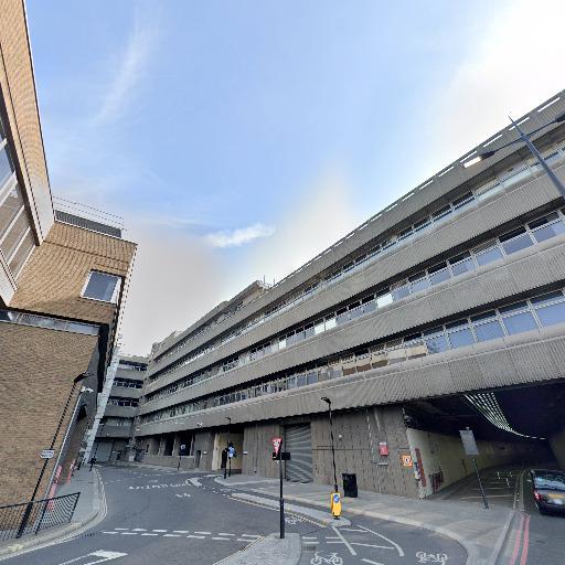
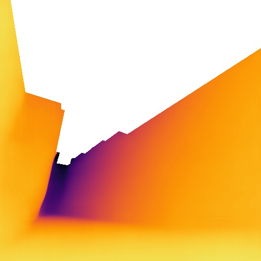
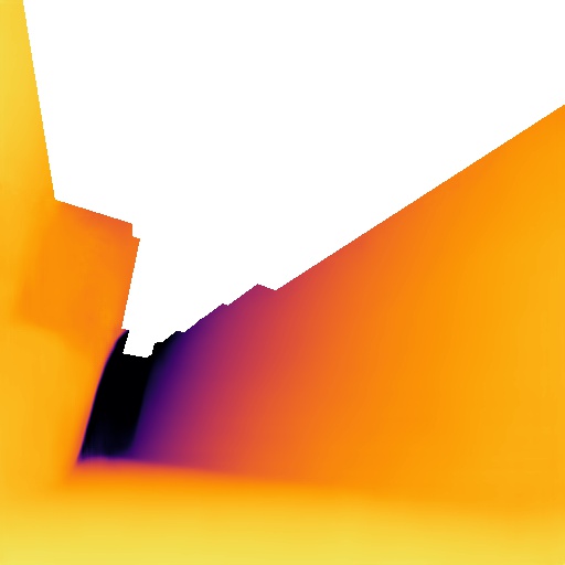
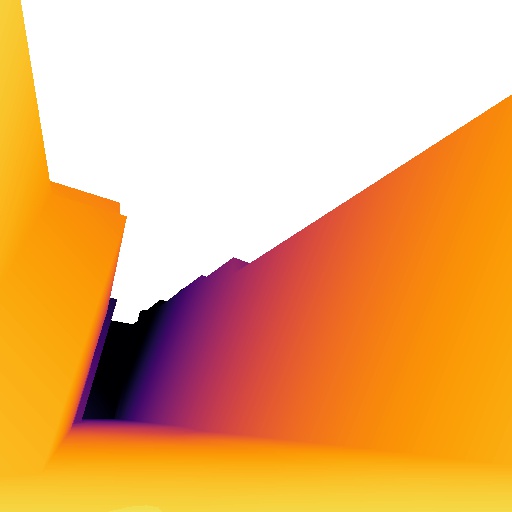
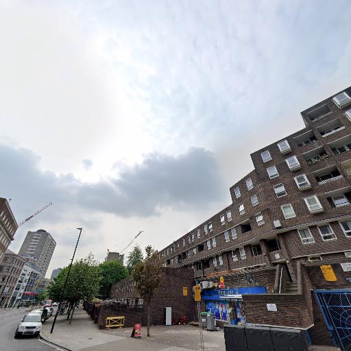
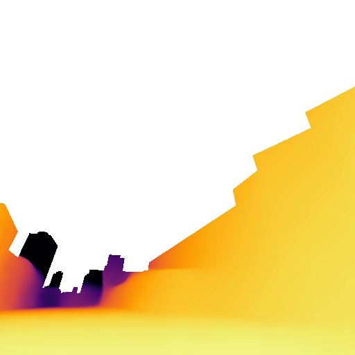
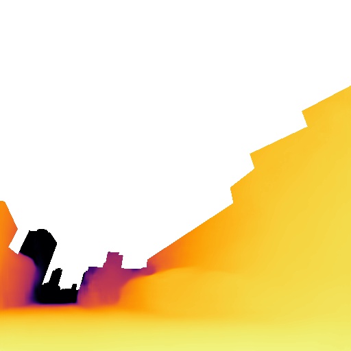
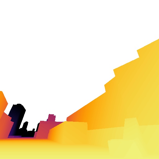
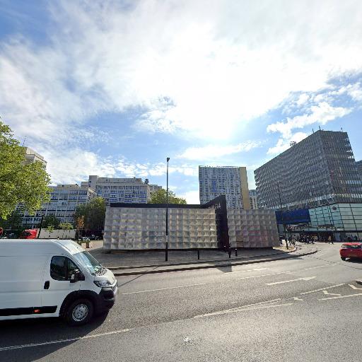
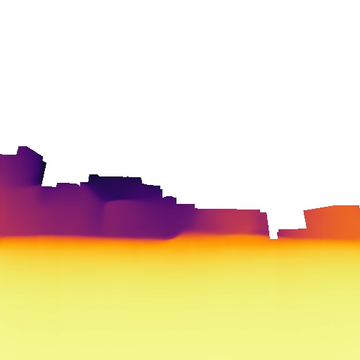
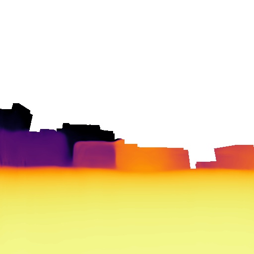
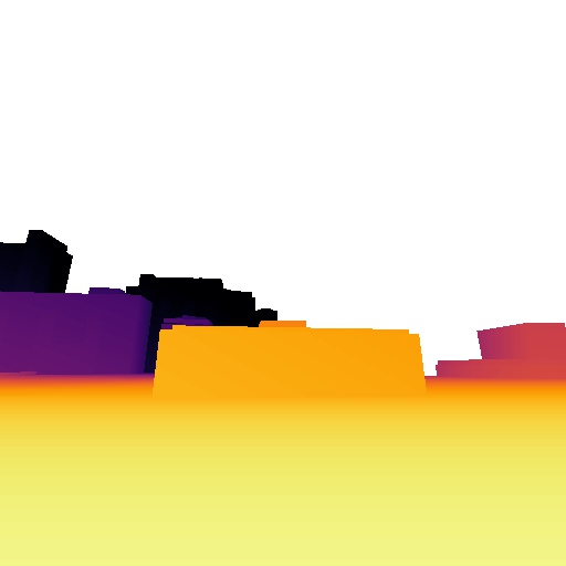
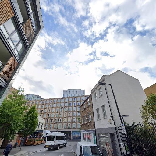
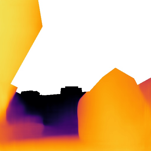
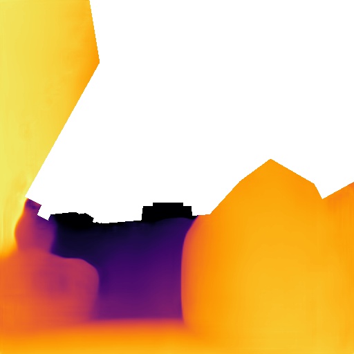
Finally, in Figure S6 we show results generated by our method alongside results from the ground-only baseline. As observed, our approach that integrates geospatial context is better able to capture the scale of the scene. For example, in the first row, the ground-only baseline significantly underestimates the maximum depth along the road compared to our approach.

3 Application: Estimating Geo-Orientation

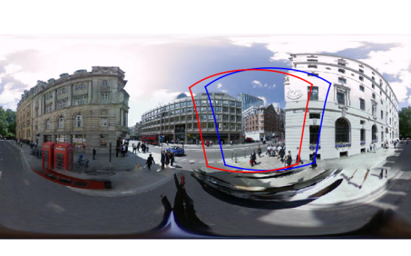
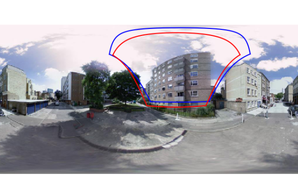
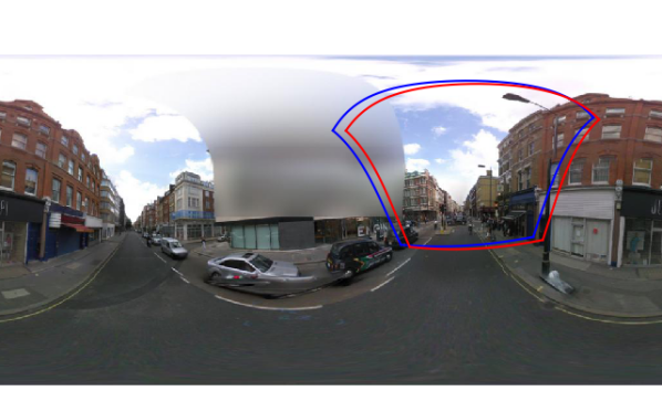
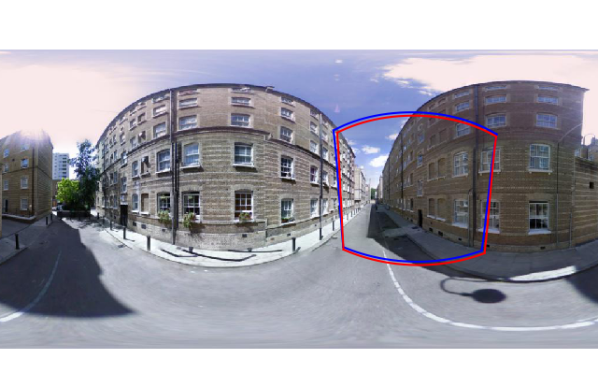
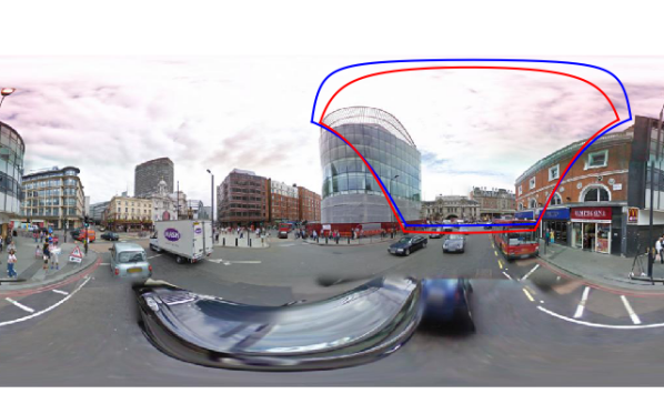
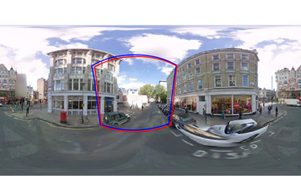
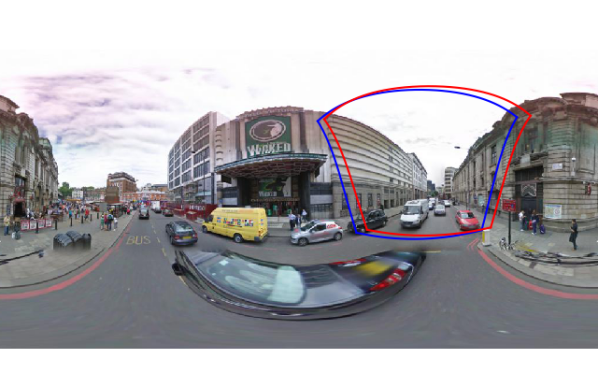
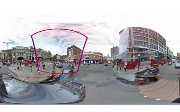
We show that our intermediate representation of scale (in the form of a synthetic depth panorama) can be used for a variety of applications, including orientation estimation. For this experiment, we use the overhead height map at zoom level 16. Given a query ground-level depth map with known geolocation but unknown orientation, we first generate the synthetic depth panorama from a co-located height map using our approach. We then perform a grid search over yaw/pitch parameters at one degree intervals, extracting the corresponding perspective depth cutout, and comparing to the query depth image. Each orientation is assigned a score using mean absolute error between the two depth maps, selecting the lowest error configuration as our prediction. Example registration results are shown in Figure S7. The ground-truth perspective cutout boundary is shown in blue and the result of our registration technique is shown in red. Despite this simple approach, the estimated orientations are quite accurate.

Figure S7: Example results from orientation estimation. The perspective image boundary corresponding to the true orientation is shown in blue and our registration result is shown in red.

References

- [1] Ibraheem Alhashim and Peter Wonka. High quality monocular depth estimation via transfer learning. arXiv preprint arXiv:1812.11941, 2018.
- [2] Amir Atapour-Abarghouei and Toby P Breckon. Real-time monocular depth estimation using synthetic data with domain adaptation via image style transfer. In IEEE Conference on Computer Vision and Pattern Recognition, 2018.
- [3] Abhishek Chaurasia and Eugenio Culurciello. LinkNet: Exploiting encoder representations for efficient semantic segmentation. In IEEE Visual Communications and Image Processing, 2017.
- [4] Weifeng Chen, Zhao Fu, Dawei Yang, and Jia Deng. Single-image depth perception in the wild. In Advances in Neural Information Processing Systems, 2016.
- [5] Erick Delage, Honglak Lee, and Andrew Y Ng. A dynamic bayesian network model for autonomous 3D reconstruction from a single indoor image. In IEEE Conference on Computer Vision and Pattern Recognition, 2006.
- [6] Jia Deng, Wei Dong, Richard Socher, Li-Jia Li, Kai Li, and Li Fei-Fei. ImageNet: A large-scale hierarchical image database. In IEEE Conference on Computer Vision and Pattern Recognition, 2009.
- [7] David Eigen, Christian Puhrsch, and Rob Fergus. Depth map prediction from a single image using a multi-scale deep network. In Advances in Neural Information Processing Systems, 2014.
- [8] WA Falcon et al. PyTorch Lightning. GitHub. Note: https://github.com/PyTorchLightning/pytorch-lightning, 3, 2019.
- [9] Huan Fu, Mingming Gong, Chaohui Wang, Kayhan Batmanghelich, and Dacheng Tao. Deep ordinal regression network for monocular depth estimation. In IEEE Conference on Computer Vision and Pattern Recognition, 2018.
- [10] Nehla Ghouaiel and Sébastien Lefèvre. Coupling ground-level panoramas and aerial imagery for change detection. Geo-spatial Information Science, 19(3):222–232, 2016.
- [11] Clément Godard, Oisin Mac Aodha, and Gabriel J Brostow. Unsupervised monocular depth estimation with left-right consistency. In IEEE Conference on Computer Vision and Pattern Recognition, 2017.
- [12] Clément Godard, Oisin Mac Aodha, Michael Firman, and Gabriel J Brostow. Digging into self-supervised monocular depth estimation. In IEEE International Conference on Computer Vision, 2019.
- [13] Kaiming He, Xiangyu Zhang, Shaoqing Ren, and Jian Sun. Deep residual learning for image recognition. In IEEE Conference on Computer Vision and Pattern Recognition, 2016.
- [14] Derek Hoiem, Alexei A Efros, and Martial Hebert. Automatic photo pop-up. In ACM Transactions on Graphics (SIGGRAPH), 2005.
- [15] Gao Huang, Zhuang Liu, Laurens Van Der Maaten, and Kilian Q Weinberger. Densely connected convolutional networks. In IEEE Conference on Computer Vision and Pattern Recognition, 2017.
- [16] Diederik Kingma and Jimmy Ba. Adam: A method for stochastic optimization. In International Conference on Learning Representations, 2014.
- [17] Manon Kok, Jeroen D Hol, and Thomas B Schön. Using inertial sensors for position and orientation estimation. arXiv preprint arXiv:1704.06053, 2017.
- [18] Iro Laina, Christian Rupprecht, Vasileios Belagiannis, Federico Tombari, and Nassir Navab. Deeper depth prediction with fully convolutional residual networks. In International Conference on 3D Vision, 2016.
- [19] Jin Han Lee, Myung-Kyu Han, Dong Wook Ko, and Il Hong Suh. From big to small: Multi-scale local planar guidance for monocular depth estimation. arXiv preprint arXiv:1907.10326, 2019.
- [20] Jae-Han Lee and Chang-Su Kim. Monocular depth estimation using relative depth maps. In IEEE Conference on Computer Vision and Pattern Recognition, 2019.
- [21] Tsung-Yi Lin, Serge Belongie, and James Hays. Cross-view image geolocalization. In IEEE Conference on Computer Vision and Pattern Recognition, 2013.
- [22] Liu Liu and Hongdong Li. Lending orientation to neural networks for cross-view geo-localization. In IEEE Conference on Computer Vision and Pattern Recognition, 2019.
- [23] Xiaohu Lu, Zuoyue Li, Zhaopeng Cui, Martin R Oswald, Marc Pollefeys, and Rongjun Qin. Geometry-aware satellite-to-ground image synthesis for urban areas. In IEEE Conference on Computer Vision and Pattern Recognition, 2020.
- [24] Jiebo Luo, Jie Yu, Dhiraj Joshi, and Wei Hao. Event recognition: Viewing the world with a third eye. In ACM International Conference on Multimedia, 2008.
- [25] Gellért Máttyus, Shenlong Wang, Sanja Fidler, and Raquel Urtasun. HD Maps: Fine-grained road segmentation by parsing ground and aerial images. In IEEE Conference on Computer Vision and Pattern Recognition, 2016.
- [26] Robert McCraith, Lukas Neumann, and Andrea Vedaldi. Calibrating self-supervised monocular depth estimation. In British Machine Vision Conference, 2020.
- [27] National Coordination Office for Space-Based Positioning, Navigation, and Timing. GPS accuracy. https://www.gps.gov/systems/gps/performance/accuracy/, 2021.
- [28] Adam Paszke, Sam Gross, Francisco Massa, Adam Lerer, James Bradbury, Gregory Chanan, Trevor Killeen, Zeming Lin, Natalia Gimelshein, Luca Antiga, et al. PyTorch: An imperative style, high-performance deep learning library. In Advances in Neural Information Processing Systems, 2019.
- [29] René Ranftl, Katrin Lasinger, David Hafner, Konrad Schindler, and Vladlen Koltun. Towards robust monocular depth estimation: Mixing datasets for zero-shot cross-dataset transfer. IEEE Transactions on Pattern Analysis and Machine Intelligence, 2020.
- [30] Md Alimoor Reza, Jana Kosecka, and Philip David. FarSight: Long-range depth estimation from outdoor images. In IEEE/RSJ International Conference on Intelligent Robots and Systems, 2018.
- [31] Mattia Rossi, Mireille El Gheche, Andreas Kuhn, and Pascal Frossard. Joint graph-based depth refinement and normal estimation. In IEEE Conference on Computer Vision and Pattern Recognition, 2020.
- [32] Tawfiq Salem, Scott Workman, and Nathan Jacobs. Learning a dynamic map of visual appearance. In IEEE Conference on Computer Vision and Pattern Recognition, 2020.
- [33] Tawfiq Salem, Menghua Zhai, Scott Workman, and Nathan Jacobs. A multimodal approach to mapping soundscapes. In IEEE International Geoscience and Remote Sensing Symposium, 2018.
- [34] Ashutosh Saxena, Min Sun, and Andrew Y Ng. Make3D: Learning 3D scene structure from a single still image. IEEE Transactions on Pattern Analysis and Machine Intelligence, 31(5):824–840, 2008.
- [35] Kevin Tang, Manohar Paluri, Li Fei-Fei, Rob Fergus, and Lubomir Bourdev. Improving image classification with location context. In IEEE International Conference on Computer Vision, 2015.
- [36] Jan D Wegner, Steven Branson, David Hall, Konrad Schindler, and Pietro Perona. Cataloging public objects using aerial and street-level images-urban trees. In IEEE Conference on Computer Vision and Pattern Recognition, 2016.
- [37] Scott Workman and Nathan Jacobs. Dynamic traffic modeling from overhead imagery. In IEEE Conference on Computer Vision and Pattern Recognition, 2020.
- [38] Scott Workman, Richard Souvenir, and Nathan Jacobs. Wide-area image geolocalization with aerial reference imagery. In IEEE International Conference on Computer Vision, 2015.
- [39] Scott Workman, Richard Souvenir, and Nathan Jacobs. Understanding and mapping natural beauty. In IEEE International Conference on Computer Vision, 2017.
- [40] Scott Workman, Menghua Zhai, David J. Crandall, and Nathan Jacobs. A unified model for near and remote sensing. In IEEE International Conference on Computer Vision, 2017.
- [41] Kai Zhang, Jiaxin Xie, Noah Snavely, and Qifeng Chen. Depth sensing beyond LiDAR range. In IEEE Conference on Computer Vision and Pattern Recognition, 2020.
- [42] Wang Zhao, Shaohui Liu, Yezhi Shu, and Yong-Jin Liu. Towards better generalization: Joint depth-pose learning without PoseNet. In IEEE Conference on Computer Vision and Pattern Recognition, 2020.
- [43] Tinghui Zhou, Matthew Brown, Noah Snavely, and David G. Lowe. Unsupervised learning of depth and ego-motion from video. In IEEE Conference on Computer Vision and Pattern Recognition, 2017.
- [44] Yichao Zhou, Jingwei Huang, Xili Dai, Linjie Luo, Zhili Chen, and Yi Ma. HoliCity: A city-scale data platform for learning holistic 3D structures. arXiv preprint arXiv:2008.03286, 2020.