Mode-by-mode Relative Binning: Fast Likelihood Estimation for Gravitational Waveforms with Spin-Orbit Precession and Multiple Harmonics
Abstract
Faster likelihood evaluation enhances the efficiency of gravitational wave signal analysis. We present Mode-by-mode Relative Binning (MRB), a new method designed for obtaining fast and accurate likelihoods for advanced waveform models that include spin-orbit precession effects and multiple radiation harmonics from compact binary coalescence. Leveraging the “twisting-up” procedure of constructing precessing waveform modes from non-precessing ones, the new method mitigates degrade of relative binning accuracy due to interference from superimposed modes. Additionally, we supplement algorithms for optimizing the choice of frequency bins specific to any given strain signal under analysis. Using the new method, we are able to evaluate the likelihood with up to an order of magnitude reduction in the number of waveform model calls per frequency compared to the previously used relative binning scheme, and achieve better likelihood accuracy than is sufficient for obtaining source parameter posterior distributions that are indistinguishable from the exact ones.
I Introduction
Astrophysical information about gravitational wave sources is commonly extracted via parameter inference within the Bayesian framework. This process requires thorough sampling of a high-dimensional parameter space (e.g. with a total of 10–15 source parameters), and hence a huge number (typically on the order of –) of likelihood evaluations. To map either the likelihood function or the posterior distribution, it is important to accurately evaluate the likelihood function on manageable timescales.
Brute-force calculation of the likelihood is often costly. In order to be compatible with Fast Fourier Transform (FFT), it requires evaluating the frequency-domain model waveform on a uniformly sampled, sufficiently fine grid that has frequencies, where is the highest frequency that includes information and is the duration of the gravitational wave signal in the sensitive frequency band of the detector. The computational cost can be especially prohibitive if is long or if is large. Even non-uniform frequency sampling still requires a large number of grid points, as the waveform phase typically evolves over a large number of cycles across the sensitive frequency band. For GW parameter inference with sophisticated waveform models, model calls at individual frequencies often dominate the runtime. For many frequency domain waveform models, the computational time of a likelihood evaluation scales nearly linearly with the number of queried frequencies [1].
A number of methods have been developed to approximate the likelihood with fewer frequency evaluations, trading an insignificantly amount of accuracy degrade for substantial speedup. Reduced order quadrature (ROQ) [1] is one such method, which pre-computes a reduced basis for a given waveform model, and approximates any physical waveform with an interpolant in the linear space spanned by this basis. This method only needs as many independent evaluations as there are basis elements, and has been applied to reduce the computational time of a variety of waveform models [2, 3, 4, 5].
Relative binning [6, 7, 8], originally developed for non-precessing waveforms in the dominant radiation mode, is another method to achieve the same goal. In relative binning, the ratio between a given waveform and an appropriately chosen fiducial waveform is considered. If the fiducial waveform is a decent fit of the data, only waveforms that resemble the fiducial one need to be examined in parameter inference, for which the waveform ratio conveniently has a milder frequency dependence. For this reason, the waveform ratio can be well approximated as a piecewise-linear function in the frequency domain, which only requires waveform model calls at the edges of a reduced number of frequency bins.
For simple waveform models with only one harmonic such as IMRPhenomD [9], this method has been shown to require fewer waveform evaluations than ROQ for the same error tolerance [6], and has been routinely used in independent analysis of public LIGO/Virgo data [10, 11, 12, 13, 14]. An earlier and somewhat similar method referred to as heterodyne, which also samples the ratio between two waveforms using fewer grid points, was proposed in Ref. [15].
Many gravitational wave sources carry a strong imprint of the effects of precession of the orbital plane, which are neglected in simpler models like IMRPhenomD. These precession effects are often accounted for by effective precession parameters that well approximate the effects with minimal additional complexity or dimensionality [16, 17, 18]. However, more sophisticated waveform models that fully incorporate the effects of spin-orbit precession with misaligned spins and higher harmonic modes [19, 20, 21, 22, 23] have begun to be widely applied in parameter inference. Compared to many of the non-precessing models, which only incorporate the dominant radiation mode, these advanced models have yielded better fits to numerical simulations [24], better fits to the detected LIGO/Virgo gravitational wave signals [25], higher SNR, more precision, and more accuracy in parameter estimation for injected signals [26, 27, 28], and in some cases have led to the intriguing discovery of new solutions [29, 30, 31, 32].
Additionally, information in higher modes is crucial in tracking the recoil kicks of the GW sources [33], and this information should be reliably extractable once LIGO/Virgo reach their design sensitivities [34].
In the original implementation of relative binning presented in Ref. [6], the key assumption is that the ratio between a waveform under examination over a fiducial one has significantly smoother frequency dependence than the waveform themselves do. The quality of this assumption however degrades for precessing waveforms with the full symphony of harmonics, as both the precession-induced wobbling of the binary orbital plane and the superposition of multiple harmonics give rise to additional oscillations with the frequency in the observed waveform. It is pivotal to realize that a precessing waveform can be decomposed into a linear combination of contributions from individual radiation harmonics in the co-precessing frame [35], and our schemes deal with ratios evaluated for these modes individually and hence only have to sample functions that are smoother in the frequency space. Our scheme builds a likelihood from piecewise linear interpolants of these smooth quantities. As an explicit example, we demonstrate this strategy using the phenomenological waveform model IMRPhenomXPHM [21, 24, 36].
In this paper, we present two improved relative binning schemes specially designed for precessing waveforms with multiple harmonics, which we jointly refer to as the Mode-by-mode Relative Binning (MRB). We give explicit formulae to approximate the likelihood, and we introduce practical algorithms to choose appropriate frequency bins. We find theoretical speedup of MRB relative to the original relative binning method by up to an order of magnitude, which is due to a reduced number of frequency bins required, for the same tolerable absolute accuracy in the log likelihood.
The rest of the paper is organized as follows. In Section II, we review the “twisting-up” procedure for building precession waveforms and introduce the basic definitions that will be used in the MRB schemes. In Section III, we present the technical details of the two MRB schemes, including introducing piecewise linear approximation for quantities that are smooth functions of the frequency, as well as new methods to optimize the frequency bins. In Section IV, we study the required number of frequency bins as a function of accuracy tolerance by applying MRB to real and injected gravitational wave signals, with a comparison to the old relative binning method without using mode decomposition. Finally, we provide discussion of our results in Section V and concluding remarks in Section VI.
II Mode decomposition for precessing waveforms
To understand how relative binning can be best applied to waveforms that describe precessing binary systems, we start by discussing the general structure of precessing waveforms. Many precessing models with higher modes are built using an approximate mapping from a non-precessing system to a precessing system, often referred to as the “twisting-up” procedure [35, 37]. This includes state-of-the-art phenomenological [20, 21] and effective one body [22] waveform models. Under the twisting-up scheme, the non-precessing waveforms resemble the gravitational radiation emitted by a non-precessing source, as if an imaginary observer is fixed relative to the wobbling orbital plane of the binary [35].
The specific prescription for twisting-up the non-precessing waveforms that we use is developed in [37] and is fully detailed for the IMRPhenomXPHM model in [21]. Here, we note the most important aspects of this prescription that will allow us to explain our schemes. A general waveform model outputs the frequency domain waveform of both polarizations, i.e. and . Models that use the twisting-up procedure include a prescription for a non-precessing waveform as what a fictitious observer would see in the co-precessing frame. This non-precessing waveform can be decomposed into building blocks, , following the spin-weighted spherical harmonic expansion. Since the binary orbital timescale is typically significantly shorter than the timescale of spin-orbit precession, the precession effects on the waveform can be well captured by a time-dependent Euler rotation of the non-precessing waveform [37]. After transforming from the time domain into the frequency domain under the stationary phase approximation, the model also provides three frequency-dependent Euler angles, , and , which parameterize a rotation from the frame co-precessing with the orbital angular momentum vector (the -frame) to the approximately inertial frame defined by the total angular momentum vector (the -frame). Using the definitions introduced in Ref. [21], it is a straightforward derivation that both polarizations can be expressed as a linear combination of the -frame modes . We follow their convention that is used to label the -frame modes, and is used to label the -frame modes.
| (1a) | |||
| (1b) |
Often, only a few subdominant modes are included in this sum as the contribution of almost all higher order modes are negligibly small. The dominant mode is always included, and the leading subdominant modes and are usually included. Our implementation and the LALSuite implementation [38] of the IMRPhenomXPHM model use these modes and the and modes. Hence, the overall waveform observed in the inertial frame is reduced to a short list of basis modes, which have simpler frequency dependence individually.
The frequency-dependent coefficients and incorporate an in-plane rotation by a frequency-independent angle , which depends on the orientation of the binary, to correct for the difference between the computed spin-weighted spherical harmonics defined with respect to the total angular momentum vector, and the conventional parameterization of the waveform defined with respect to the reference orbital angular momentum vector.
| (2a) | |||
| (2b) |
The tilded coefficients are specified in terms of the frequency-dependent Euler angles , and , as well as , the constant angle between the total angular momentum vector and the line of sight:
| (3a) | |||
| (3b) |
where ∗ stands for complex conjugation, and we introduce the following coefficient to describe the mixing between the -frame modes and the -frame modes under precession:
| (4) |
Here, is the Wigner small -matrix element evaluated at the Euler angle , and is the spin-weighted spherical harmonic.
Finally, the observed strain at a given detector is a linear combination of the two wave polarizations and . The linear coefficients are given by the detector response coefficients, and , which are dependent on the sky position of the gravitational wave source and the orientation of the detector at the time of the gravitational wave event. The detector response coefficients depend on three extrinsic parameters: right ascension , declination , and the polarization angle . In the frequency domain, the arrival time of the event introduces a phase that scales linearly with the frequency.
| (5) |
The overall result is that the strain observed at a given detector can be cast into the following linear combination of the non-precessing modes,
| (6) |
where
| (7) |
Two additional definitions are convenient for discussion in the following sections. First, we can absorb the arrival time dependence into the -frame mode to define the time-dependent quantity
| (8) |
for which we simply have
| (9) |
Second, we can incorporate the coefficient and define the full mode component
| (10) |
The observed waveform then has the simple decomposition
| (11) |
III Mode-by-mode Relative Binning Schemes
As mentioned in Section I, the original relative binning scheme assumes that the full waveform divided by a fiducial waveform is smooth in frequency space so that it can be well approximated by a piecewise linear interpolant. This scheme was developed for non-precessing waveform models that only account for the dominant mode. When applied to these waveform models, the assumption of the original relative binning scheme is only that the ratio of the mode evaluated for any given parameters over the mode evaluated at a fiducial set of parameters is a smooth function of the frequency. If the original relative binning method is applied to a precessing waveform comprised of multiple modes, this assumption is being extended to the sum of all modes, which is a stronger assumption. Instead, we improve our accuracy by not extending this assumption and only applying it to individual non-precessing modes.
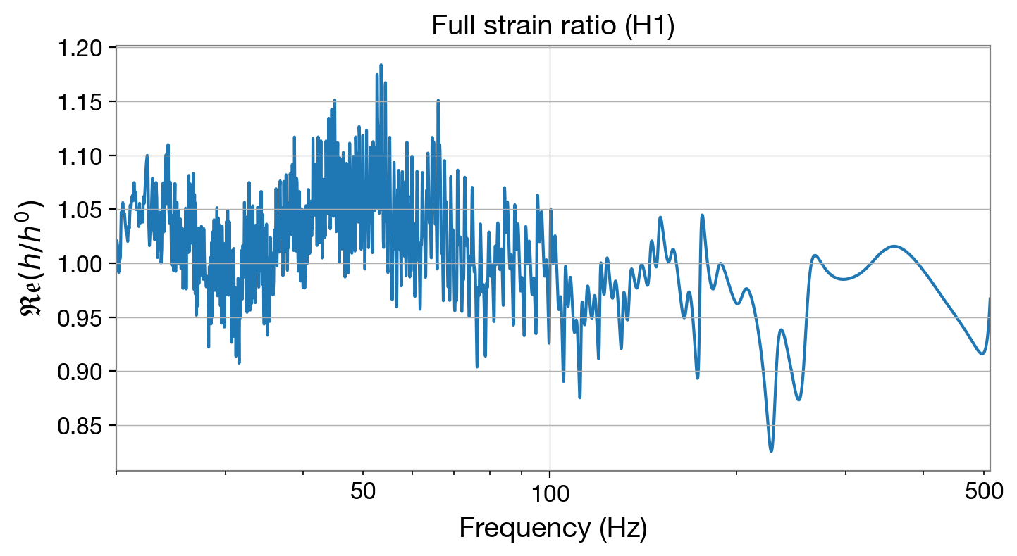
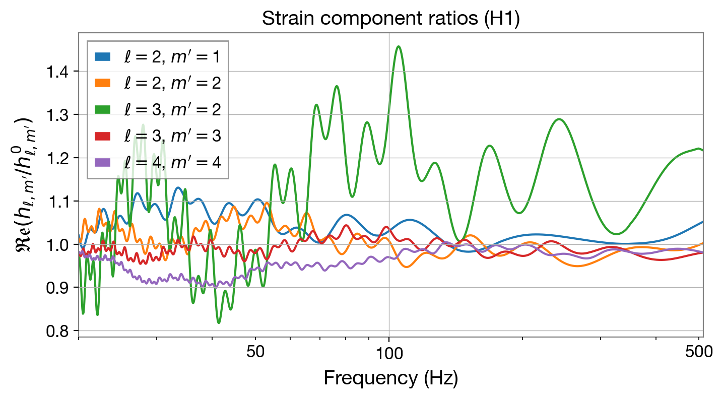
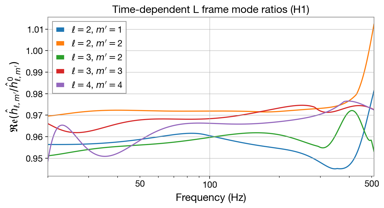
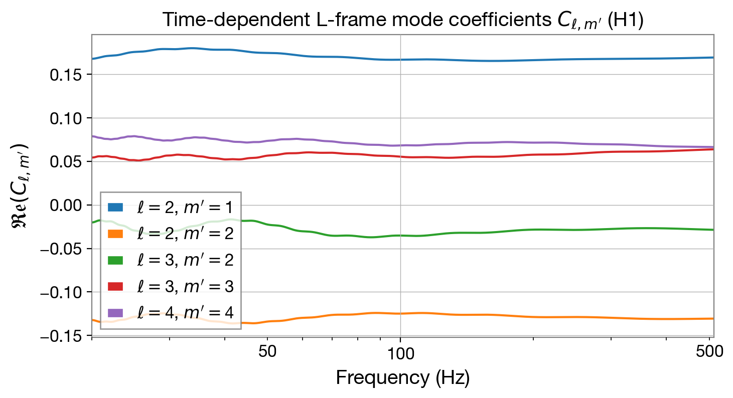
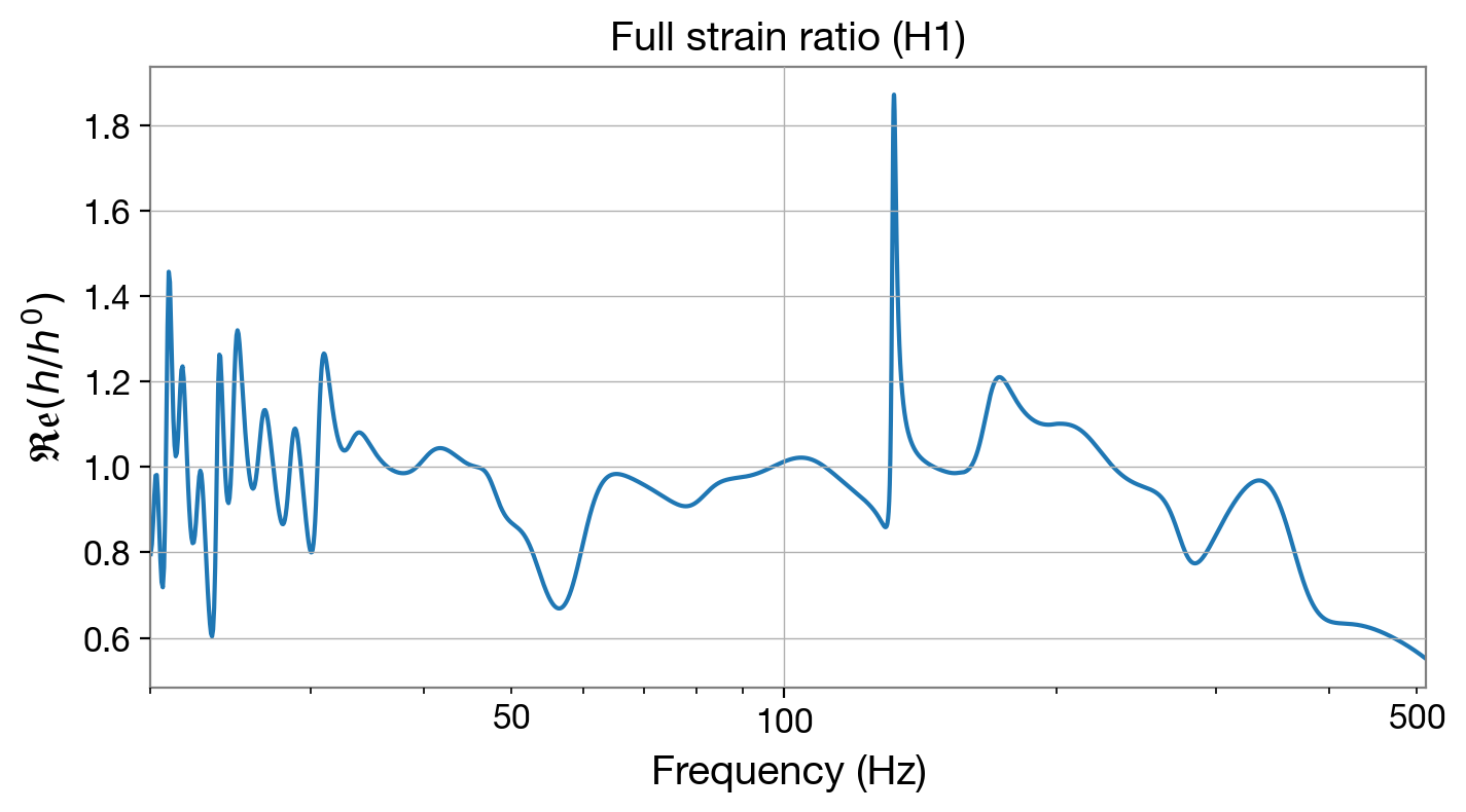
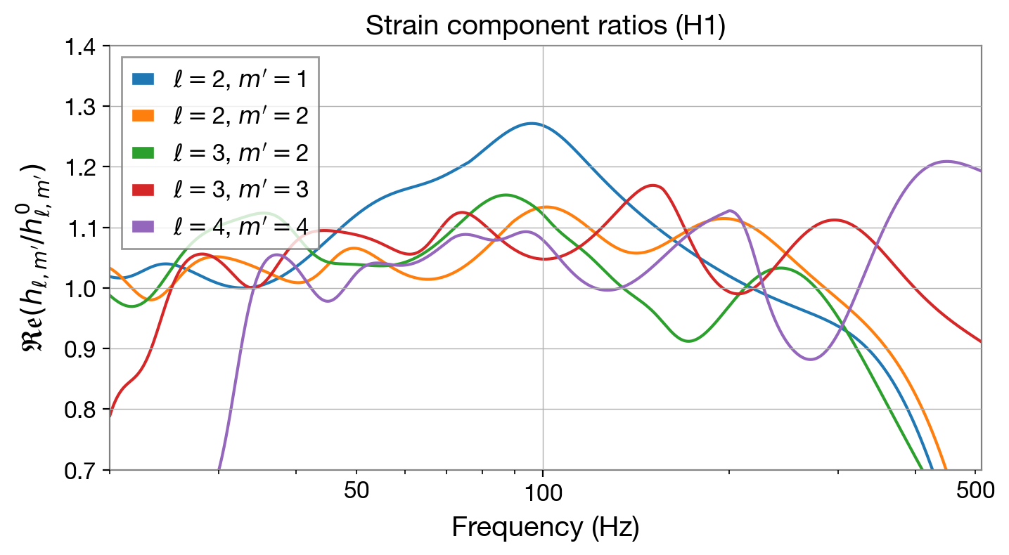
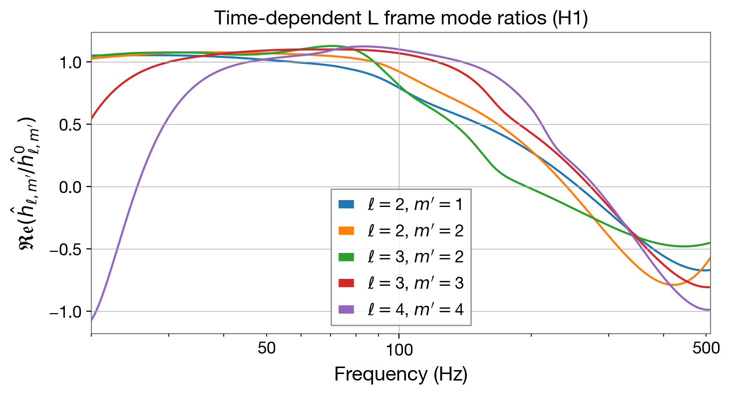
At a fixed orbital frequency, the various -frame modes produced by a binary source have different frequencies, and hence their superposition exhibit interference features. This leads to a jagged ratio for the overall waveform, , as a function of the frequency, as we exemplify in the top panel of Figure 1. The lower three panels in Figure 1, by contrast, show the smoother quantities , defined in Eq. (10), , defined in Eq. (8), and , defined in Eq. (7), which are associated with individual -frame modes. We will instead approximate these quantities or their ratios over fiducial counterparts by piecewise linear interpolants in our two schemes.
 |
 |
 |
 |
III.1 Scheme 1
In the first scheme, we handle each time-dependent -frame mode as we handle the full waveform in the original relative binning method. To this end, we decompose the fiducial waveform as
| (12) |
In this scheme, we suitably create frequency bins which we label by . Within each frequency bin, the ratio of the time-dependent -frame mode over some fiducial one is well approximated by a linear interpolant:
| (13) |
where is the frequency at the bin center. The coefficients and , defined for every frequency bin, are found by computing the waveform ratio at the bin edges. The speedup of relative binning hence comes from the fact that it suffices to evaluate at the bin edges for an excellent approximation of the likelihood. To obtain the full waveform , we also need the frequency dependent coefficients, which we also linearize within each frequency bin:
| (14) |
The constant coefficient in the piecewise linear interpolant of () is not to be confused with the fiducial (). We disambiguate by showing that the former is a function of bin and waveform , and the latter is a function of frequency . Likewise, the coefficients and can be computed from evaluated at the bin edges. In practice, we find that both quantities are smooth functions of the frequency, as shown in Figure 1. We then need to compute the likelihood in terms of these linearized ratios and coefficients. The log likelihood for the data series, , given a signal series , is given by:
| (15) |
where is the notation for the standard complex-valued overlaps defined via a summation over only positive frequencies :
| (16a) | |||
| (16b) |
where is one-sided power spectral density (PSD) of the detector noise, and is the length of time series analyzed.
To approximate the above overlaps, we introduce a number of summary data for each frequency bin. The coefficients are used in the overlap and are associated with a single -frame mode because they are linear in the strain . The coefficients are used in the overlap and are associated with a pair of -frame modes because they are quadratic in the strain .
| (17a) | |||
| (17b) | |||
| (17c) | |||
| (17d) |
These summary data only depend on the data series and the chosen fiducial waveform, and hence can be computed in advance of the large number of likelihood evaluations required in the sampling process. To obtain the log likelihood at each sampled set of waveform parameters, we approximate the overlaps up to linear order in , using the following sums over frequency bins
| (18a) | ||||
| (18b) | ||||
To summarize, the summary data Eq. (17d) can be pre-computed from the data and the chosen fiducial waveform; then to approximate the log likelihood using Eq. (18) and Eq. (15), , , , and only need to be evaluated at the bin edges.
III.2 Scheme 2
Scheme 1 involves the multiplication of two quantities, both of which are separately approximated as piecewise linear functions. One might wonder if this strategy accumulates excessive errors. Hence, we consider an alternative scheme, which we refer to as Scheme 2. In this scheme, we linearize the ratio of the entire mode component over its fiducial counterpart. To do so, we decompose the fiducial waveform as in Eq. (11):
| (19) |
Within the frequency bin , we make the approximation
| (20) |
This quantity is also much smoother than the ratio for the observed waveform, which is linearized in the original relative binning method, as one can see in Figure 1. In this scheme, our summary data are very similar, but they use the full fiducial mode components:
| (21a) | |||
| (21b) | |||
| (21c) | |||
| (21d) |
Now that there is only one linearized quantity, the overlaps have shorter expressions:
| (22a) | |||
| (22b) | |||
Again, the pre-computed summary data Eq. (21d) can be substituted into Eq. (22) to compute the overlaps Eq. (16b) up to linear order in . The coefficients and only require evaluating the model waveform at the edges of the frequency bins. Although Scheme 2 have simpler expressions than Scheme 1, it is not meaningfully faster in terms of the computation runtime, as all evaluations needed for computing and are also needed for computing .
III.3 Bin Selection
Previously, a prescription to determine the frequency bins for the original relative binning method is presented in Ref. [6]. Motivated by the post-Newtonian expansion, this prescription selects frequency bins to bound the differential phase changes assuming a phenomenological ansatz in the form of a sum over power-law phases. Although the prescription has the advantage that it is independent of the specific compact binary coalescence signals under analysis, it may not be the optimized bin selection on the event-by-event basis. In particular, for high binary masses, the merger and ringdown signals may dominate the sensitive frequency band of the detector, and the corresponding gravitational wave signal may be poorly described by the post-Newtonian expansion.
In this work, we present a new bin selection algorithm that is adaptive to any given gravitational wave signal under investigation. Since the linearized quantities associated with individual modes have smoother frequency dependence than the observed waveform, we can afford fewer frequency bins to achieve a comparable accuracy for the log likelihood. Since the bottleneck in the computational time cost is still the large number of likelihood evaluations, we can afford to adjust the frequency bins event by event via an algorithm that is more time-consuming than the one that is adopted in Ref. [6]. We choose a representative waveform (different from the fiducial waveform) for an estimate of the binning errors. We can then test out various binning choices on this representative waveform. Methods for choosing this waveform are discussed in Section V.
Our algorithm determines the frequency bins by starting with the entire frequency range as a single bin and iteratively bisecting the frequency bins. In this iterative process, we compute, for each existing frequency bin, the error contribution to the log likelihood due to mode-by-mode relative binning. We keep bisecting the bins until the overall absolute error in the log likelihood is smaller than a empirically set threshold. We iterate the whole procedure and update the target number of bins to the number of bins achieved in the previous run, until the resulting number of bins and the target number of bins converge. This algorithm is detailed in Algorithm 1.
The algorithm consistently converges to a fixed number of bins independent of the initial target number of bins (targetN), so we set this number arbitrarily to 200. By varying the total allowed error on the test parameters, we trade computational cost (number of bins) for accuracy. We tested similar algorithms that unevenly divide the bins, but found that such methods are slower and did not improve accuracy.
IV Testing Methods and Results
We tested the accuracy and efficiency of both mode-by-mode relative binning schemes on several real and synthetic compact binary coalescence events. We computed likelihoods of the IMRPhenomXPHM model using LALSuite [38] and gathered posterior samples using the MultiNest sampler [39].
To test our method, we consider gravitational wave signals with either strong spin-orbit precession or large contributions from the subdominant modes, or a combination of both, as their parameter estimation can be greatly improved with IMRPhenomXPHM or other precessing models with higher modes that exploit the twisting-up procedure. Precession occurs most dramatically in binaries that have large spin vectors misaligned with the binary orbital angular momentum vector (i.e. large in-plane spin components) [40]. Odd parity subdominant modes such as are important when there is a large asymmetry between the two components, e.g. when the mass ratio is small. Also, subdominant modes are larger in the late stage of the merger. For low mass mergers, the most sensitive LIGO/Virgo frequency band corresponds to the early inspiral of the merger. On the contrary, for heavy mass mergers, the most sensitive frequency band corresponds to the merger stage when subdominant modes are stronger. For these reasons, we study events with large in-plane spin components, or a small mass ratio , or a large total mass.
We consider one real LIGO/Virgo event, GW190814, and four injected events. GW190814 is chosen because the original analysis shows strong Bayesian evidence favoring a model that includes the mode over one that has only the dominant mode [30]. The four injections are chosen as the following. Two are chosen to resemble the inferred source properties of two interesting LIGO/Virgo detections for which new source solutions have been recently reported from independent reanalyses using the IMRPhenomXPHM model: GW151226 [41, 31] and GW190521 [42, 32]. Both of these newly found solutions indicate a large spin misaligned with the orbital angular momentum on the primary mass and a low mass ratio . The GW151226 reanalysis showed that the new low- solution were absent from the posterior distribution of the source parameters when either the higher modes or the precession effects were neglected [31]. The original analysis of GW190521 used the IMRPhenomPv3HM model [20], which had higher modes and precession, but not the improved calibration of the subdominant modes, and particularly not in the low- regime [42, 32]. The other two injections are artificially made to have a high total mass and large in-plane spins: one with a high mass ratio and another with a low mass ratio. The parameters used for the injections are listed in Table 1.
| High | Low | GW151226-like | GW190521-like | GW190814 (fiducial) | |
|---|---|---|---|---|---|
| Primary mass [] | 30.0 | 100.0 | 29.3 | 168.0 | 24.4 |
| Secondary mass [] | 20.0 | 10.0 | 4.3 | 16.0 | 2.7 |
| 0.700 | 0.700 | 0.600 | 0.641 | 0.024 | |
| 0.000 | 0.000 | -0.200 | 0.000 | 0.039 | |
| 0.000 | 0.000 | 0.500 | -0.559 | 0.002 | |
| 0.000 | 0.000 | 0.000 | 0.000 | -0.305 | |
| 0.700 | 0.700 | 0.000 | 0.000 | -0.574 | |
| 0.000 | 0.000 | 0.000 | 0.000 | -0.067 | |
| Luminosity distance [Mpc] | 496.91 | 496.91 | 457.00 | 400.00 | 283.28 |
| Line of sight [rad] | 1.200 | 1.200 | 0.403 | 0.500 | 2.408 |
| 111As defined in Appendix C of Ref. [21] | 0.200 | 0.200 | 0.000 | 0.000 | 2.730 |
| Right ascension [rad] | 3.000 | 3.000 | 3.831 | 3.340 | 0.412 |
| Declination [rad] | 0.100 | 0.100 | -0.819 | 0.600 | -0.574 |
| Polarization angle [rad] | 0.500 | 0.500 | 2.698 | 0.000 | 2.962 |
| GPS time | 1242443867.4 | 1242443867.4 | 1135137260.6 | 1242443867.4 | 1249852257.0 |
To start with, we need posterior source parameters for which we can evaluate the log likelihood both approximately using our new mode-by-mode binning method and exactly. The samples are collected using MultiNest with . For these runs, the log likelihoods are evaluated using the original relative binning method of Ref. [6]. We use the parameter choice for the maximum allowed differential phase (see Eq. 10 of Ref. [6] for the definition of ), which is sufficient for obtaining accurate posterior samples. For the injected events, the injected parameters are used to set the fiducial waveform. For the real GW190814 event, fiducial parameters are found using scipy’s differential_evolution [43], a global optimization routine to (approximately) find the maximum likelihood fit to the data.
We obtain the strain data containing GW190814, as well as those used as the noisy background for our injections, from the public database GWOSC [44]. For each event, we collect a 16-second time series centered on the GPS time listed in Table 1 with a sampling rate of 1024 Hz. The injections are added at the 8 second mark into the noisy 16-second time series. PSDs are measured using Welch’s method from a 128-second time series centered at the same GPS time with overlapping 16 s segments. We only include frequencies from 20 Hz to 512 Hz in the likelihood evaluation, as there is negligible SNR contribution outside this frequency range.
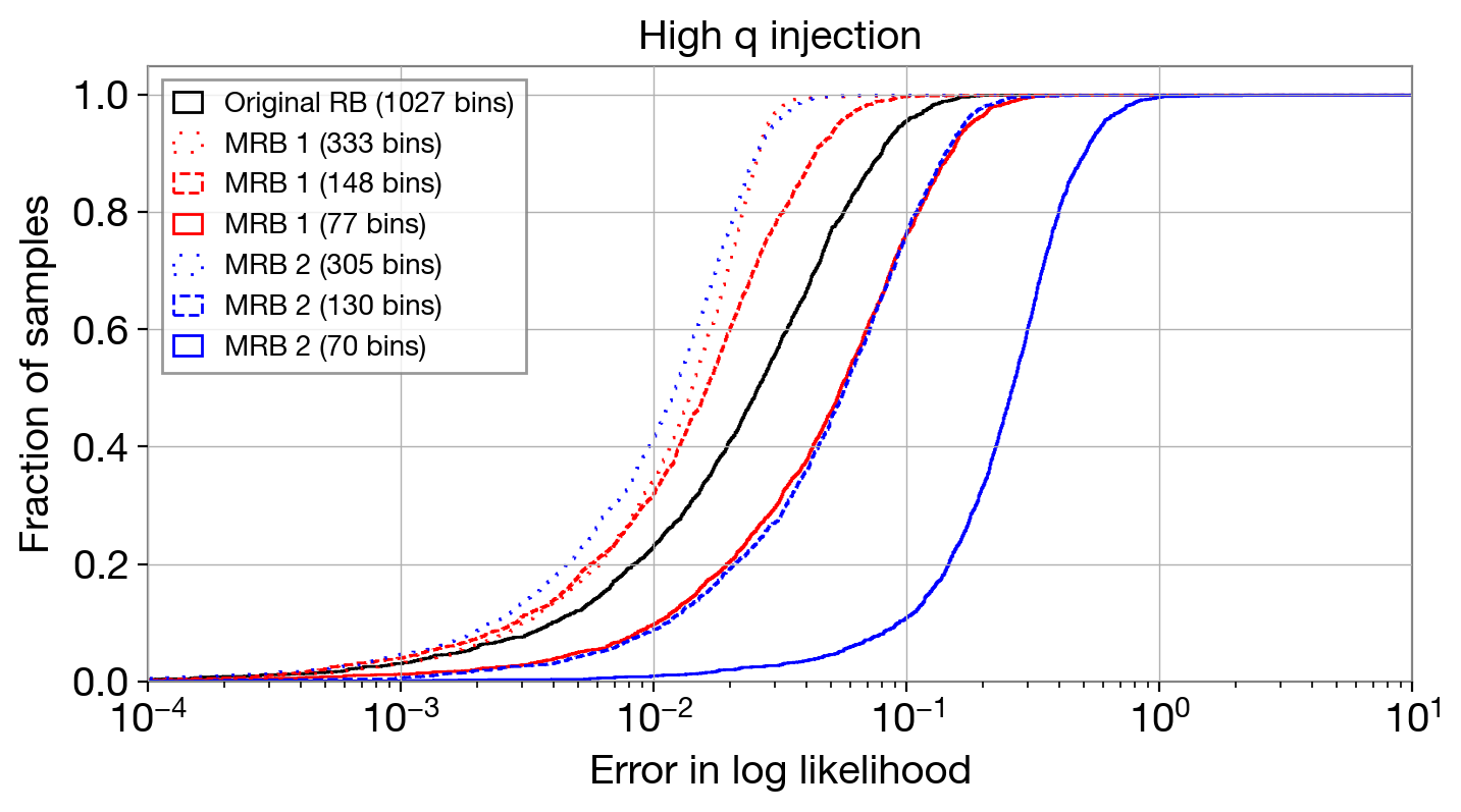
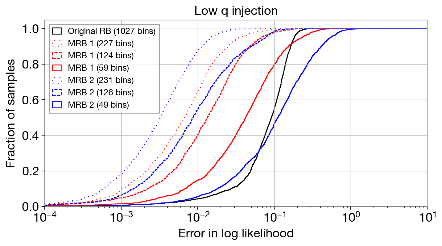
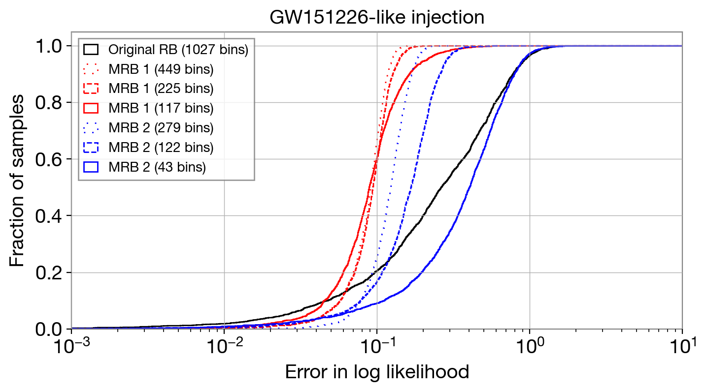
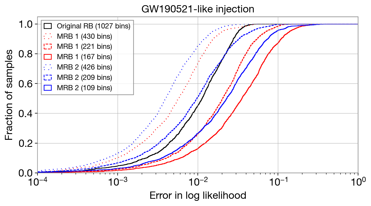
We make a comparison between the original relative binning method using the original bin selection algorithm (with the parameter as defined in Ref. [6]), and the mode-by-mode relative binning method using our new bin selection (for a range of values), evaluating for 2000 parameter combinations randomly drawn from the posterior distribution derived for each event or injection. The bin selection algorithm uses a random posterior sample selected as the test waveform. We study the absolute errors in the log likelihood computed for these samples, which are shown in Figure 2 and Figure 3.
 |
 |
 |
 |
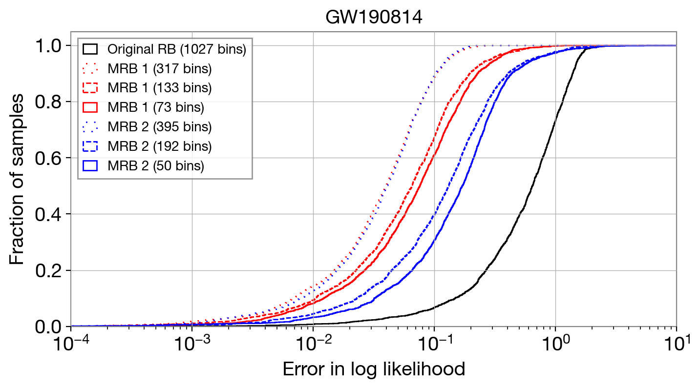 |
Figure 2 and Figure 3 show the cumulative distribution function (CDF) for the absolute error in the log likelihood for the 2000 posterior samples collected for each event. We compare the original relative binning method with mode-by-mode relative binning, testing both our approximation schemes and varying . The varying numbers of bins result from using different values. The number of frequency bins is one less than the number of required frequency-domain waveform evaluations, which dominate the runtime, so the bin number is a good proxy for the runtime. In all examples we show, the original relative binning method uses the same number of frequency bins because the bin selection prescription only depends on the frequency range and the maximum differential phase , which do not change from event to event.
In Appendix A, we investigate the tolerable size of the absolute error in the log likelihood for obtaining accurate posterior distributions. Conservatively, we conclude that the log likelihood error should be no greater than as random errors with a standard deviation of appear to have unnoticeable effect in the posterior.
For the high injection, and using only 148 bins with Scheme 1, the errors with mode-by-mode relative binning (MRB) are smaller than those with the original relative binning method using 1027 bins at all percentiles. Using about 300 bins, both Scheme 1 and Scheme 2 are able to achieve this. Notably, these three cases have the log likelihood error no greater than 0.1 for all samples.
Similarly, for the low injection, the MRB error derived from about 125 bins strictly outperforms that of the original relative binning. The error distribution has a larger standard deviation than in the high case, but this is due to most of low error samples having even smaller errors.
For all methods, the samples for the GW151226-like injection have larger errors, but using 117 bins with Scheme 1 the error is less than 0.1 for 60% of the samples, and using more bins the spread of the worse errors is significantly reduced, and the error is nearly always less than 0.2 for roughly twice the number of bins.
The GW190521-like injection is the only example studied here where Scheme 2 achieves lower errors than Scheme 1 does using comparable number of bins. Nevertheless, Scheme 1 achieves lower errors than the original relative binning scheme with 430 bins. For the GW190814 event, 90% of the errors are less than 0.1, when using 300–400 bins with both Scheme 1 and Scheme 2. The errors are roughly a factor of two to four larger using only 73 bins under Scheme 1. In the 317 bin case, Scheme 1 reduces the error by nearly an order of magnitude at one third of the computational cost when compared with original relative binning.
Overall, both MRB schemes achieve lower errors with fewer bins at all percentiles above 50% when compared with the original relative binning method. In all cases, MRB achieves a median absolute error of 0.1 using substantially reduced number of bins.
V Discussion
In all cases except the GW190521-like injection, Scheme 1 outperforms Scheme 2. We believe this is because the quantities linearized in Scheme 1 are usually smoother functions of the frequency than those linearized in Scheme 2, which reduces the required number of bins for a given accuracy goal. This can be seen in Figure 1. In fact, the ratio linearized in Scheme 2 is related to the one linearized in Scheme 1 through
| (23) | |||||
The ratio linearized in Scheme 1 is similar to the ratio linearized in the original relative binning method applied to non-precessing waveform models. The -frame mode components are equivalent to the -frame components for a non-precessing waveform, and it has already been demonstrated that the ratio of non-precessing waveforms are smooth in the frequency space. However, the ratio can exhibit large oscillations or even sharp peaks when the denominator becomes small. This situation may arise because the coefficient is a linear combination of terms that may nearly cancel (see construction of in Section II).
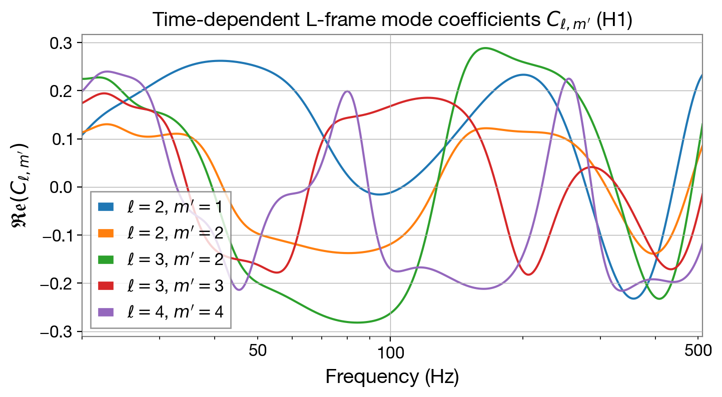
However, it can also happen that Scheme 2 outperforms Scheme 1. When the aforementioned issue regarding does not arise, Scheme 2 may have an advantage because there are fewer quantities to be linearized so as to avoid compounding error. This appears to be the case in the GW190521-like injected event. The linearized quantities evaluated for one posterior sample of this event are compared in Figure 4. In this example, Scheme 1 is not advantageous over Scheme 2 in terms of frequency-space smoothness of the linearized quantities.
Overall, we conclude that Scheme 1 is more robust because it accounts for the difficult case of small , and more often yields better relative binning results, especially in the case of GW190814. In practice, the preferred scheme can be empirically determined alongside the process of choosing suitable fiducial and test waveforms.
 |
 |
 |
 |
To use mode-by-mode relative binning in practice, one has to set a fiducial waveform for computing the summary data, and a test waveform for determining the frequency bins. If the experimental collaboration has already provided full parameter inference results for the event under analysis, the reported parameters can be used as the fiducial parameters. If the signal under analysis is uncovered by a search pipeline, crude source masses and spins are typically reported, and can be used as the initial choice for the fiducial parameters. If not all parameters are reported, or are only reported for simplified waveform models, then the fiducial parameters can be obtained via global maximization of the exact likelihood. For well measured parameters, global optimization should be performed within the small vicinity of the reported values. For poorly measured parameters, optimization can performed over the entire physically allowed region.
If global optimization using the exact likelihood is computationally too slow, it is feasible to couple the relative binning approximation to the optimization. If the likelihood errors from using the initial choice of ficudial parameters are still too large, the fiducial parameters can be iteratively updated, just like what has been practiced using the original relative binning method [6, 7]. As a matter of fact, there is great flexibility in setting the fiducial parameters, as many extrinsic parameters enter the individual modes only through frequency independent factors which do not degrade the accuracy of mode-by-mode relative binning.
Our results are minimally affected when changing which sample is used as the test waveform for the selection of frequency bins. This suggests that any set of test parameters in the support of the posterior distribution would be satisfactory. In practice, we recommend obtaining the test parameters by running a few iterations of a sampler starting from the fiducial parameters. The test parameters can be obtained by a few Metropolis-Hastings iterations, or a few steps of a more sophisticated sampler running on the exact log likelihood.
VI Conclusion
In this paper, we address faster likelihood evaluations, one important aspect of speeding up gravitational wave parameter inference among several factors including sampling efficiency and parallel capabilities. We have developed the mode-by-mode relative binning method as an efficient approximation of the likelihood function, and have demonstrated its enhanced accuracy and theoretical speedup compared with the original relative binning method that does not take advantage of the multi-modal structure of the waveform.
The existing implementation can be found in our git repository at https://github.com/nathaniel-leslie/modebymode-relative-binning. With an optimized implementation applied to spin-orbit precessing waveforms including multiple harmonic modes, we expect the mode-by-mode relative binning method to run faster than comparable reduced order quadratures. An ROQ has been built for IMRPhenomXPHM using a code called PyROQ [45]. To evaluate the likelihood with ROQ, one must evaluate the linear and quadratic overlaps, which correspond to Eq. (16a) and Eq. (16b) respectively. Each overlap requires an interpolant to be evaluated, which requires the number of waveform evaluations that is equal to the number of basis functions for each interpolant. In Table III of [45], it is shown that the total number of basis functions in their ROQ for IMRPhenomXPHM with a signal up to 1024 Hz ranged from 600 to 1100, depending on the parameter ranges. As shown in Figure 2 and Figure 3, mode-by-mode relative binning can achieve the conservative target of absolute errors in the log likelihood error being around 0.1 on all test events with only around 100–200 frequency bins.
Another benefit of mode-by-mode relative binning is the ability to vary to flexibly trade speed for accuracy. This only requires recomputing bins by rerunning Algorithm 1 with a new value of , which takes a few seconds. If one achieves sufficient accuracy for a specific problem and can afford to sacrifice some, can be increased, which reduces bin count and runtime. Similarly, if one requires higher accuracy and can afford some additional runtime, can be decreased, which increases bin count and runtime but also improves accuracy.
Our conclusions about runtime are based on the reduction in the number of waveform evaluations, and nearly equivalently, the number of frequency bins. As we have mentioned previously, this is justified by the observation that waveform evaluation calls dominate the computational time of the likelihood evaluation. In the code used in this work, and for the IMRPhenomXPHM waveform model as an example, we have computed the -frame modes and the Euler angles , , and by calling the available LALSuite routines [38]. These routines take approximately 3/4 of the time of a full likelihood evaluation using the full LALSuite routines for obtaining and . The remaining time is primarily spent on computing the twisting factors and , which involves a significant amount of evaluations of trigonometric functions and scales linearly with the bin number. Our current Python implementation of mode-by-mode relative binning is still inefficient due to overhead; it takes a few milliseconds to compute these twisting factors even for a few frequencies. The existing LALSuite routines for obtaining and are sufficient for implementing the original relative binning method, which do not require computations of the twisting factors in Python. For this method, with 1027 bins, each likelihood evaluation takes roughly - ms on a 2018 MacBook Pro with a 2.6 GHz Intel i7 processor. The time that it takes to evaluate the -frame modes and Euler angles at the original bins is also about 3/4 of this time. We expect that an optimized routine coded in C, Julia, optimized Python packages, or in some other programming languages could realize such a performance. For the 133 bin evaluation shown in Figure 3, the -frame modes and Euler angles took approximately 0.7 ms. Assuming optimized implementation of the twisting factors, the same extrapolation suggests that sub-millisecond likelihood evaluations are achievable.
The fast evaluation times of the LALSuite code relative to our Python implementation demonstrate that the theoretical speed improvements of our code are realizable. In order to realize the full potential of mode by mode relative binning, this optimization must be performed. Once this is achieved, this method shows promise for substantially reducing the computational cost of parameter estimation for precessing waveforms with higher modes.
This method has only been tested on IMRPhenomXPHM, but we expect it to be similarly effective for other frequency-domain models with higher modes and precession. A simple application of this method to native time-domain models like TEOBResumS [46] runs into a number of difficulties. Transforming these models into the frequency domain can be prohibitively slow, so one would hope to evaluate the likelihood in the time domain. In the time domain, the likelihood function becomes more than a simple frequency sum, as stationary noise produces a non-diagonal covariance matrix in the time domain. This particularly becomes difficult for relative binning with the term, as it would necessarily require sums over two time indices for each sampled waveform. New techniques will be needed to leverage the advantages of relative binning for these kinds of models. We are currently developing such relative binning methods for these time-domain models, and we hope to present tests of these methods in a following paper.
Acknowledgements.
VII Acknowledgements
We would like to thank Uroš Seljak and Biwei Dai for useful discussions. NL is supported by N3AS under National Science Foundation grant PHY-1630782. LD acknowledges the research grant support from the Alfred P. Sloan Foundation (award number FG-2021-16495). GP is supported by STFC, the School of Physics and Astronomy at the University of Birmingham and the Institute for Gravitational Wave Astronomy.
This research has made use of data, software and/or web tools obtained from the Gravitational Wave Open Science Center (https://www.gw-openscience.org/ ), a service of LIGO Laboratory, the LIGO Scientific Collaboration and the Virgo Collaboration. LIGO Laboratory and Advanced LIGO are funded by the United States National Science Foundation (NSF) as well as the Science and Technology Facilities Council (STFC) of the United Kingdom, the Max-Planck-Society (MPS), and the State of Niedersachsen/Germany for support of the construction of Advanced LIGO and construction and operation of the GEO600 detector. Additional support for Advanced LIGO was provided by the Australian Research Council. Virgo is funded, through the European Gravitational Observatory (EGO), by the French Centre National de Recherche Scientifique (CNRS), the Italian Instituto Nazionale di Fisica Nucleare (INFN) and the Dutch Nikhef, with contributions by institutions from Belgium, Germany, Greece, Hungary, Ireland, Japan, Monaco, Poland, Portugal, Spain.
Appendix A Target Log Likelihood Error
The absolute error in the log likelihood from mode-by-mode relative binning should be small enough not to bias the obtained posterior distribution for the source parameters. In this appendix, we study the impacts of log likelihood errors on the posterior distributions, using the high- injection as an example.
Our posterior samples have been obtained using the original relative binning method with finite likelihood errors. To obtain the exact (full FFT) posterior distribution, we use the method of importance sampling (IS). Let sample have the exact posterior
| (24) |
where is the exact likelihood, is the prior, and is the evidence. Using the original relative binning method, we have
| (25) |
where is the relative binning likelihood. Importance sampling requires that samples are weighted by the ratio of the desired distribution over the sampled one, so to get samples of the exact posterior, each sample has the weight
| (26) |
We can also use importance sampling to simulate specific errors in the log likelihood. The distribution of the log likelihood errors due to either relative binning method is approximately Gaussian, so we can model these errors as Gaussian random variables. Let these errors be called ; one is drawn for each sample from a Gaussian distribution. Then our simulated log likelihood with this error is
| (27) |
So following Eq. (26), the weight for the sample from this simulated distribution is
| (28) |
The above weights can be used to generate altered posteriors for comparison with an exact posterior. Such comparisons along with a histogram of the log likelihoods are shown for our high posterior in th top 4 panels of Figure 5. When the errors have a standard deviation of 0.1, they make virtually no visible impact in the posterior whatsoever. The simulated posteriors with log likelihood errors of standard deviation 0.5 and 1.0 have small inconsistencies, but their contours are generally unaltered in shape. However, once the standard deviation of the simulated error reaches 2.0, the contours are substantially distorted.

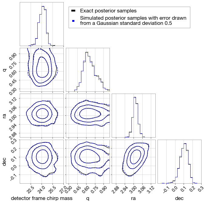
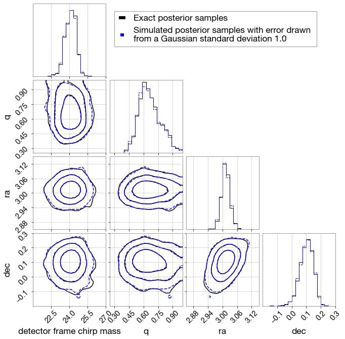
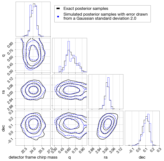
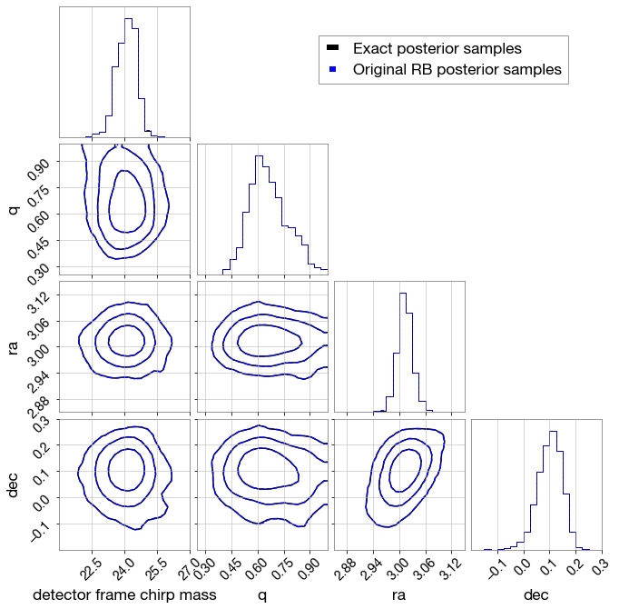
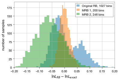
Additionally, in the bottom left of Figure 5, the actual posterior gathered from the original relative binning method and the importance weighted exact (full FFT) posterior do not differ at all. As can be seen in the blue histogram in the bottom right panel of Figure 5, the spread of the original relative binning errors log likelihood is a about 0.1.
In this example, we see that original relative binning error with a spread of about 0.1 is sufficiently small to not impact the posterior. Additionally the effect of the Gaussian error was negligible on the posterior at the same scale, and minimal up to an order of magnitude higher. Because this is only one event, we will be conservative, and use 0.1 as our target threshold, which is well justified by all of these results.
References
- Canizares et al. [2015] P. Canizares, S. E. Field, J. Gair, V. Raymond, R. Smith, and M. Tiglio, Accelerated gravitational wave parameter estimation with reduced order modeling, Physical Review Letters 114, 10.1103/physrevlett.114.071104 (2015).
- Smith et al. [2016] R. Smith, S. E. Field, K. Blackburn, C.-J. Haster, M. Pürrer, V. Raymond, and P. Schmidt, Fast and accurate inference on gravitational waves from precessing compact binaries, Physical Review D 94, 10.1103/physrevd.94.044031 (2016).
- Pürrer [2016] M. Pürrer, Frequency domain reduced order model of aligned-spin effective-one-body waveforms with generic mass ratios and spins, Physical Review D 93, 10.1103/physrevd.93.064041 (2016).
- Smith et al. [2021] R. Smith, S. Borhanian, B. Sathyaprakash, F. H. Vivanco, S. Field, P. Lasky, I. Mandel, S. Morisaki, D. Ottaway, B. Slagmolen, E. Thrane, D. Töyrä, and S. Vitale, Bayesian inference for gravitational waves from binary neutron star mergers in third-generation observatories (2021), arXiv:2103.12274 [gr-qc] .
- Morisaki and Raymond [2020] S. Morisaki and V. Raymond, Rapid parameter estimation of gravitational waves from binary neutron star coalescence using focused reduced order quadrature, Physical Review D 102, 10.1103/physrevd.102.104020 (2020).
- Zackay et al. [2018] B. Zackay, L. Dai, and T. Venumadhav, Relative binning and fast likelihood evaluation for gravitational wave parameter estimation (2018), arXiv:1806.08792 [astro-ph.IM] .
- Dai et al. [2018] L. Dai, T. Venumadhav, and B. Zackay, Parameter estimation for gw170817 using relative binning (2018), arXiv:1806.08793 [gr-qc] .
- Finstad and Brown [2020] D. Finstad and D. A. Brown, Fast parameter estimation of binary mergers for multimessenger follow-up, The Astrophysical Journal 905, L9 (2020).
- Khan et al. [2016] S. Khan, S. Husa, M. Hannam, F. Ohme, M. Pürrer, X. J. Forteza, and A. Bohé, Frequency-domain gravitational waves from nonprecessing black-hole binaries. ii. a phenomenological model for the advanced detector era, Physical Review D 93, 10.1103/physrevd.93.044007 (2016).
- Zackay et al. [2019] B. Zackay, T. Venumadhav, L. Dai, J. Roulet, and M. Zaldarriaga, Highly spinning and aligned binary black hole merger in the Advanced LIGO first observing run, Phys. Rev. D 100, 023007 (2019), arXiv:1902.10331 [astro-ph.HE] .
- Venumadhav et al. [2019] T. Venumadhav, B. Zackay, J. Roulet, L. Dai, and M. Zaldarriaga, New search pipeline for compact binary mergers: Results for binary black holes in the first observing run of Advanced LIGO, Phys. Rev. D 100, 023011 (2019), arXiv:1902.10341 [astro-ph.IM] .
- Roulet et al. [2020] J. Roulet, T. Venumadhav, B. Zackay, L. Dai, and M. Zaldarriaga, Binary black hole mergers from ligo/virgo o1 and o2: Population inference combining confident and marginal events, Physical Review D 102, 10.1103/physrevd.102.123022 (2020).
- Roulet et al. [2021] J. Roulet, H. S. Chia, S. Olsen, L. Dai, T. Venumadhav, B. Zackay, and M. Zaldarriaga, On the distribution of effective spins and masses of binary black holes from the ligo and virgo o1-o3a observing runs (2021), arXiv:2105.10580 [astro-ph.HE] .
- Nitz et al. [2021] A. H. Nitz, C. D. Capano, S. Kumar, Y.-F. Wang, S. Kastha, M. Schäfer, R. Dhurkunde, and M. Cabero, 3-ogc: Catalog of gravitational waves from compact-binary mergers (2021), arXiv:2105.09151 [astro-ph.HE] .
- Cornish [2013] N. J. Cornish, Fast fisher matrices and lazy likelihoods (2013), arXiv:1007.4820 [gr-qc] .
- Schmidt et al. [2015] P. Schmidt, F. Ohme, and M. Hannam, Towards models of gravitational waveforms from generic binaries: Ii. modelling precession effects with a single effective precession parameter, Physical Review D 91, 10.1103/physrevd.91.024043 (2015).
- Gerosa et al. [2021] D. Gerosa, M. Mould, D. Gangardt, P. Schmidt, G. Pratten, and L. M. Thomas, A generalized precession parameter to interpret gravitational-wave data, Physical Review D 103, 10.1103/physrevd.103.064067 (2021).
- Thomas et al. [2021] L. M. Thomas, P. Schmidt, and G. Pratten, New effective precession spin for modeling multimodal gravitational waveforms in the strong-field regime, Physical Review D 103, 10.1103/physrevd.103.083022 (2021).
- Hannam et al. [2014] M. Hannam, P. Schmidt, A. Bohé, L. Haegel, S. Husa, F. Ohme, G. Pratten, and M. Pürrer, Simple model of complete precessing black-hole-binary gravitational waveforms, Physical Review Letters 113, 10.1103/physrevlett.113.151101 (2014).
- Khan et al. [2020] S. Khan, F. Ohme, K. Chatziioannou, and M. Hannam, Including higher order multipoles in gravitational-wave models for precessing binary black holes, Physical Review D 101, 10.1103/physrevd.101.024056 (2020).
- Pratten et al. [2020a] G. Pratten, C. García-Quirós, M. Colleoni, A. Ramos-Buades, H. Estellés, M. Mateu-Lucena, R. Jaume, M. Haney, D. Keitel, J. E. Thompson, and S. Husa, Let’s twist again: computationally efficient models for the dominant and sub-dominant harmonic modes of precessing binary black holes (2020a), arXiv:2004.06503 [gr-qc] .
- Ossokine et al. [2020] S. Ossokine, A. Buonanno, S. Marsat, R. Cotesta, S. Babak, T. Dietrich, R. Haas, I. Hinder, H. P. Pfeiffer, M. Pürrer, and et al., Multipolar effective-one-body waveforms for precessing binary black holes: Construction and validation, Physical Review D 102, 10.1103/physrevd.102.044055 (2020).
- Varma et al. [2019] V. Varma, S. E. Field, M. A. Scheel, J. Blackman, D. Gerosa, L. C. Stein, L. E. Kidder, and H. P. Pfeiffer, Surrogate models for precessing binary black hole simulations with unequal masses, Physical Review Research 1, 10.1103/physrevresearch.1.033015 (2019).
- García-Quirós et al. [2020] C. García-Quirós, M. Colleoni, S. Husa, H. Estellés, G. Pratten, A. Ramos-Buades, M. Mateu-Lucena, and R. Jaume, Multimode frequency-domain model for the gravitational wave signal from nonprecessing black-hole binaries, Phys. Rev. D 102, 064002 (2020), arXiv:2001.10914 [gr-qc] .
- Chatziioannou et al. [2019] K. Chatziioannou, R. Cotesta, S. Ghonge, J. Lange, K. K. Ng, J. Calderón Bustillo, J. Clark, C.-J. Haster, S. Khan, M. Pürrer, and et al., On the properties of the massive binary black hole merger gw170729, Physical Review D 100, 10.1103/physrevd.100.104015 (2019).
- Kalaghatgi et al. [2020] C. Kalaghatgi, M. Hannam, and V. Raymond, Parameter estimation with a spinning multimode waveform model, Physical Review D 101, 10.1103/physrevd.101.103004 (2020).
- Shaik et al. [2020] F. H. Shaik, J. Lange, S. E. Field, R. O’Shaughnessy, V. Varma, L. E. Kidder, H. P. Pfeiffer, and D. Wysocki, Impact of subdominant modes on the interpretation of gravitational-wave signals from heavy binary black hole systems, Physical Review D 101, 10.1103/physrevd.101.124054 (2020).
- Graff et al. [2015] P. B. Graff, A. Buonanno, and B. Sathyaprakash, Missing link: Bayesian detection and measurement of intermediate-mass black-hole binaries, Physical Review D 92, 10.1103/physrevd.92.022002 (2015).
- Mateu-Lucena et al. [2021] M. Mateu-Lucena, S. Husa, M. Colleoni, H. Estellés, C. García-Quirós, D. Keitel, M. de Lluc Planas, and A. Ramos-Buades, Adding harmonics to the interpretation of the black hole mergers of gwtc-1 (2021), arXiv:2105.05960 [gr-qc] .
- Abbott et al. [2020a] R. Abbott, T. D. Abbott, S. Abraham, F. Acernese, K. Ackley, C. Adams, R. X. Adhikari, V. B. Adya, C. Affeldt, M. Agathos, and et al., Gw190814: Gravitational waves from the coalescence of a 23 solar mass black hole with a 2.6 solar mass compact object, The Astrophysical Journal 896, L44 (2020a).
- Chia et al. [2021] H. S. Chia, S. Olsen, J. Roulet, L. Dai, T. Venumadhav, B. Zackay, and M. Zaldarriaga, Boxing day surprise: Higher multipoles and orbital precession in gw151226 (2021), arXiv:2105.06486 [astro-ph.HE] .
- Nitz and Capano [2021] A. H. Nitz and C. D. Capano, Gw190521 may be an intermediate-mass ratio inspiral, The Astrophysical Journal 907, L9 (2021).
- Calderón Bustillo et al. [2018] J. Calderón Bustillo, J. A. Clark, P. Laguna, and D. Shoemaker, Tracking black hole kicks from gravitational-wave observations, Physical Review Letters 121, 10.1103/physrevlett.121.191102 (2018).
- Varma et al. [2020] V. Varma, M. Isi, and S. Biscoveanu, Extracting the gravitational recoil from black hole merger signals, Physical Review Letters 124, 10.1103/physrevlett.124.101104 (2020).
- Schmidt et al. [2011] P. Schmidt, M. Hannam, S. Husa, and P. Ajith, Tracking the precession of compact binaries from their gravitational-wave signal, Phys. Rev. D 84, 024046 (2011), arXiv:1012.2879 [gr-qc] .
- Pratten et al. [2020b] G. Pratten, S. Husa, C. Garcia-Quiros, M. Colleoni, A. Ramos-Buades, H. Estelles, and R. Jaume, Setting the cornerstone for a family of models for gravitational waves from compact binaries: The dominant harmonic for nonprecessing quasicircular black holes, Phys. Rev. D 102, 064001 (2020b), arXiv:2001.11412 [gr-qc] .
- Schmidt et al. [2012] P. Schmidt, M. Hannam, and S. Husa, Towards models of gravitational waveforms from generic binaries: A simple approximate mapping between precessing and nonprecessing inspiral signals, Physical Review D 86, 10.1103/physrevd.86.104063 (2012).
- LIGO Scientific Collaboration [2018] LIGO Scientific Collaboration, LIGO Algorithm Library - LALSuite, free software (GPL) (2018).
- Feroz et al. [2009] F. Feroz, M. P. Hobson, and M. Bridges, Multinest: an efficient and robust bayesian inference tool for cosmology and particle physics, Monthly Notices of the Royal Astronomical Society 398, 1601–1614 (2009).
- Apostolatos et al. [1994] T. A. Apostolatos, C. Cutler, G. J. Sussman, and K. S. Thorne, Spin-induced orbital precession and its modulation of the gravitational waveforms from merging binaries (1994).
- Abbott et al. [2016] B. Abbott, R. Abbott, T. Abbott, M. Abernathy, F. Acernese, K. Ackley, C. Adams, T. Adams, P. Addesso, R. Adhikari, and et al., Gw151226: Observation of gravitational waves from a 22-solar-mass binary black hole coalescence, Physical Review Letters 116, 10.1103/physrevlett.116.241103 (2016).
- Abbott et al. [2020b] R. Abbott, T. Abbott, S. Abraham, F. Acernese, K. Ackley, C. Adams, R. Adhikari, V. Adya, C. Affeldt, M. Agathos, and et al., Gw190521: A binary black hole merger with a total mass of 150 , Physical Review Letters 125, 10.1103/physrevlett.125.101102 (2020b).
- Storn and Price [1997] R. Storn and K. Price, Differential evolution – a simple and efficient heuristic for global optimization over continuous spaces, Journal of Global Optimization 11, 341 (1997).
- Rich Abbott et al. [2021] Rich Abbott, Thomas D. Abbott, Sheelu Abraham, Fausto Acernese, Kendall Ackley, Carl Adams, Rana X. Adhikari, Vaishali B. Adya, Christoph Affeldt, Michalis Agathos, and et al., Open data from the first and second observing runs of advanced ligo and advanced virgo, SoftwareX 13, 100658 (2021).
- Qi and Raymond [2021] H. Qi and V. Raymond, Pyroq: a python-based reduced order quadrature building code for fast gravitational wave inference (2021), arXiv:2009.13812 [gr-qc] .
- Nagar et al. [2018] A. Nagar, S. Bernuzzi, W. Del Pozzo, G. Riemenschneider, S. Akcay, G. Carullo, P. Fleig, S. Babak, K. W. Tsang, M. Colleoni, and et al., Time-domain effective-one-body gravitational waveforms for coalescing compact binaries with nonprecessing spins, tides, and self-spin effects, Physical Review D 98, 10.1103/physrevd.98.104052 (2018).