Robust Multi-Robot Active Target Tracking
Against Sensing and Communication Attacks

Lifeng Zhou,  and Vijay Kumar L. Zhou and V. Kumar are with the GRASP Laboratory, University of Pennsylvania, Philadelphia, PA, USA (email: {lfzhou, kumar}@seas.upenn.edu).This research was sponsored by the Army Research Lab through ARL DCIST CRA W911NF-17-2-0181.
Abstract

The problem of multi-robot target tracking asks for actively planning the joint motion of robots to track targets. In this paper, we focus on such target tracking problems in adversarial environments, where attacks or failures may deactivate robots’ sensors and communications. In contrast to the previous works that consider no attacks or sensing attacks only, we formalize the first robust multi-robot tracking framework that accounts for any fixed numbers of worst-case sensing and communication attacks. To secure against such attacks, we design the first robust planning algorithm, named Robust Active Target Tracking (RATT), which approximates the communication attacks to equivalent sensing attacks and then optimizes against the approximated and original sensing attacks. We show that RATT provides provable suboptimality bounds on the tracking quality for any non-decreasing objective function. Our analysis utilizes the notations of curvature for set functions introduced in combinatorial optimization. In addition, RATT runs in polynomial time and terminates with the same running time as state-of-the-art algorithms for (non-robust) target tracking. Finally, we evaluate RATT with both qualitative and quantitative simulations across various scenarios. In the evaluations, RATT exhibits a tracking quality that is near-optimal and superior to varying non-robust heuristics. We also demonstrate RATT’s superiority and robustness against varying attack models (e.g.. worst-case and bounded rational attacks).

Index Terms:
Multi-Robot Systems; Active Target Tracking; Robotics in Adversarial Environments; Algorithm Design & Analysis; Combinatorial Optimization.

I Introduction

Detecting, localizing, and tracking targets is central to various robotic applications such as surveillance, monitoring, and exploration. Typical examples include:

  • Area monitoring: Localize and track invasive fish (e.g., carp) in a lake; [1]

  • Search and rescue: Search and explore a burning building to localize the trapped people inside; [2]

  • Adversarial agent tracking: Detect and follow adversarial agents that try to escape in an urban environment. [3]

Such application scenarios can greatly gain from deploying multiple robots that act as mobile sensors and collaboratively plan their actions. The problem of planning the motion of a team of robots to track targets is known as multi-robot active target tracking in the literature [4]. This problem is challenging since the targets can be mobile and their motion model is generally partially known [5, 6, 7, 8, 9, 10]. The targets may move adversarially or deliberately release spoofing signals to avoid the detection and tracking of robots [11, 12]. The targets may be indistinguishable and their number may be unknown and varying over time [13]. Nevertheless, researchers have designed a number of algorithms that achieve near-optimal target tracking while tackling all of the aforementioned challenges [5, 6, 7, 8, 9, 10, 11, 12, 13].
Refer to caption
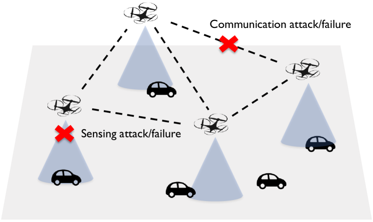
Figure 1: Adversarial target tracking: a team of aerial robots is tasked to track multiple ground vehicles in an adversarial environment, where the attacks/failures can disable robots’ sensors (e.g., block the camera’s field of view) and cut off their communications.

However, most robotics studies draw little attention to robustifying target tracking against attacks and failures that may disable robots’ sensors (e.g., cameras’ field of view may be blocked) and/or communications (e.g., communications may be jammed and disrupted); see also Fig. 1. For example, [11] focuses on cooperative planning for robots to capture multiple evaders that move adversarially to escape, instead of considering attacks that may disable robots’ sensors or communications; [12] focuses on distributed state estimation against adversaries that broadcast deceptive sensing information to mislead robots, instead of securing against adversaries that may deactivate the sensors of robots; [14] focuses on adaptive resource reconfiguration to recover robots’ resources (e.g., sensing capabilities) from failures, instead of robust algorithms that aim to withstand attacks or failures.

Recently, a number of related studies have investigated robust target tracking against attacks or failures that result in a withdrawal of robots or their sensors. For instance, [15] proposes a robust coordination algorithm that ensures provably near-optimal tracking even though some robots are attacked and their tracking sensors are disabled. [16, 17] extend the attack-robust algorithm [15] to a constrained communication scenario where robots can only communicate locally. In particular, [16, 17] propose distributed robust planning algorithms that utilize respectively the divide-and-conquer and consensus-based mechanisms to achieve robust coordination against robot or sensor attacks. Following this line, [18] presents an adaptive attack-robust algorithm against sensing attacks/failures during information acquisition tasks such as target tracking, map exploration, and area surveillance. Notably, all of these studies capitalize on recent algorithmic results on robust combinatorial optimization for set functions against subset attacks [19].

Contributions. In this paper, unlike the aforementioned works, we aim to investigate robust target tracking that accounts for both sensing and communication attacks/failures. To this end, we make four key contributions as follows.

1. Problem. We formalize the problem of robust active target tracking against worst-case sensing and communication attacks/failures. The problem asks for jointly optimizing robots’ control inputs in the presence of worst-case attacks that could disable robots’ sensing and communications. The upper bounds on the numbers of sensing and communication attacks are assumed known and fixed. To the best of our knowledge, this is the first work to formalize this problem.

2. Solution. We design the first robust algorithm, named Robust Active Target Tracking (RATT), for tackling the problem. In particular, RATT first approximates the number of communication attacks to an equivalent number of sensing attacks, and then leverages the algorithmic results in [15, 19] for robust target tracking against total sensing attacks (i.e., the original and approximated sensing attacks).

3. Analysis. We prove RATT has two main properties.

  • RATT provides suboptimality guarantees for any target tracking objective function that is 1) non-decreasing and 2) non-decreasing and submodular. The analysis of RATT’s approximation bounds is based on the notations of curvature (e.g., curvature [20] and total curvature [21]) from combinatorial optimization.

  • RATT ends with the same running time as state-of-the-art algorithms for non-robust target tracking [22, 8]) and robust target tracking against sensing attacks only [15].

4. Evaluation. We demonstrate with qualitative and quantitative simulations both the necessity for robust target tracking and RATT’s robustness against sensing and communication attacks. We show RATT exhibits superior performance against worst-case attacks and retains its superiority against non-worst-case attacks, e.g., bounded rational attack, across various scenarios.

Overall, in this paper we go beyond non-robust target tracking [6, 8, 13] by proposing robust target tracking; and beyond robust target tracking against sensing attacks only [15, 16, 18] by focusing against both sensing and communication attacks.

II Problem Formulation

We formalize the problem of robust multi-robot active target tracking. Particularly, the problem asks for choosing control inputs for robots to optimize the team tracking quality despite sensing and communication attacks/failures. To this end, we start by defining the notations used in the paper.

Notation. Calligraphic fonts denote sets (e.g., 𝒳𝒳{\mathcal{X}}). Given a set 𝒳𝒳{\mathcal{X}}, |𝒳|𝒳|{\mathcal{X}}| denotes its cardinality; 2𝒳superscript2𝒳2^{{\mathcal{X}}} denotes its power set. Lowercase or uppercase letters (e.g., x𝑥x or X𝑋X), bold lowercase letters (e.g., 𝐱𝐱{\mathbf{x}}), and bold uppercase letters (e.g., 𝐗𝐗{\mathbf{X}}) denote scalars, vectors, and matrices, respectively. 𝒳𝒴𝒳𝒴\mathcal{X}\setminus\mathcal{Y} denotes the elements in 𝒳𝒳\mathcal{X} not in 𝒴𝒴\mathcal{Y}.

Next, we first introduce the framework with some basic conventions and then formally define the problem.

II-A Framework

Robots

We consider a target tracking scenario where a team of N𝑁N mobile robots, denoted by 𝒱={1,,N}𝒱1𝑁\mathcal{V}=\{1,\cdots,N\}, is tasked to track multiple targets. Each robot i𝒱𝑖𝒱i\in\mathcal{V} has a discrete-time motion model:

𝐱i,t+1=fi(𝐱i,t,𝐮i,t),i𝒱,formulae-sequencesubscript𝐱𝑖𝑡1subscript𝑓𝑖subscript𝐱𝑖𝑡subscript𝐮𝑖𝑡for-all𝑖𝒱{\mathbf{x}}_{i,t+1}=f_{i}({\mathbf{x}}_{i,t},{\mathbf{u}}_{i,t}),~{}\forall i\in\mathcal{V}, (1)

where 𝐱isubscript𝐱𝑖{\mathbf{x}}_{i} denotes the state of robot i𝑖i and 𝐮i𝒰isubscript𝐮𝑖subscript𝒰𝑖{\mathbf{u}}_{i}\in\mathcal{U}_{i} denotes its control input. 𝒰isubscript𝒰𝑖\mathcal{U}_{i} is a finite set of available control inputs where robot i𝑖i can choose from.

Targets

We consider there are M𝑀M targets, denoted by 𝒯={1,,M}𝒯1𝑀\mathcal{T}=\{1,\cdots,M\}, to be tracked by the robots. Each target j𝒯𝑗𝒯j\in\mathcal{T} moves randomly with a stochastic motion model:

𝐲j,t+1=g(𝐲j,t)+𝐰j,t,j𝒯,formulae-sequencesubscript𝐲𝑗𝑡1𝑔subscript𝐲𝑗𝑡subscript𝐰𝑗𝑡for-all𝑗𝒯{\mathbf{y}}_{j,t+1}=g({\mathbf{y}}_{j,t})+{\mathbf{w}}_{j,t},~{}\forall j\in\mathcal{T}, (2)

where 𝐲jsubscript𝐲𝑗{\mathbf{y}}_{j} denotes the state of target j𝑗j and 𝐰j,tsubscript𝐰𝑗𝑡{\mathbf{w}}_{j,t} denotes the zero-mean white Gaussian process noise with covariance 𝐐j,tsubscript𝐐𝑗𝑡{\mathbf{Q}}_{j,t}, i.e., 𝐰j,t𝒩(0,𝐐j,t)similar-tosubscript𝐰𝑗𝑡𝒩0subscript𝐐𝑗𝑡{\mathbf{w}}_{j,t}\sim\mathcal{N}(0,{\mathbf{Q}}_{j,t}). We assume 𝐰j,tsubscript𝐰𝑗𝑡{\mathbf{w}}_{j,t} to be independent of the process noises of other targets.

Sensing

We consider a robot i𝒱𝑖𝒱i\in\mathcal{V} makes an observation of a target j𝒯𝑗𝒯j\in{\mathcal{T}} by the following measurement model:

𝐳i,tj=hij(𝐱i,t,𝐲j,t)+𝐯i,tj(𝐱i,t,𝐲j,t),i𝒱,j𝒯,formulae-sequencesuperscriptsubscript𝐳𝑖𝑡𝑗superscriptsubscript𝑖𝑗subscript𝐱𝑖𝑡subscript𝐲𝑗𝑡superscriptsubscript𝐯𝑖𝑡𝑗subscript𝐱𝑖𝑡subscript𝐲𝑗𝑡formulae-sequence𝑖𝒱𝑗𝒯{\mathbf{z}}_{i,t}^{j}=h_{i}^{j}({\mathbf{x}}_{i,t},{\mathbf{y}}_{j,t})+{\mathbf{v}}_{i,t}^{j}({\mathbf{x}}_{i,t},{\mathbf{y}}_{j,t}),~{}i\in{\mathcal{V}},j\in{\mathcal{T}}, (3)

where 𝐳i,tjsuperscriptsubscript𝐳𝑖𝑡𝑗{\mathbf{z}}_{i,t}^{j} denotes the measurement of target j𝑗j obtained by robot i𝑖i’s on-board sensor and 𝐯i,tj(𝐱i,t,𝐲j,t)superscriptsubscript𝐯𝑖𝑡𝑗subscript𝐱𝑖𝑡subscript𝐲𝑗𝑡{\mathbf{v}}_{i,t}^{j}({\mathbf{x}}_{i,t},{\mathbf{y}}_{j,t}) denotes the zero-mean white Gaussian measurement noise with covariance 𝐑(𝐱i,t,𝐲j,t)𝐑subscript𝐱𝑖𝑡subscript𝐲𝑗𝑡{\mathbf{R}}({\mathbf{x}}_{i,t},{\mathbf{y}}_{j,t}), i.e., 𝐯i,tj(𝐱i,t,𝐲j,t)𝒩(0,𝐑(𝐱i,t,𝐲j,t))similar-tosuperscriptsubscript𝐯𝑖𝑡𝑗subscript𝐱𝑖𝑡subscript𝐲𝑗𝑡𝒩0𝐑subscript𝐱𝑖𝑡subscript𝐲𝑗𝑡{\mathbf{v}}_{i,t}^{j}({\mathbf{x}}_{i,t},{\mathbf{y}}_{j,t})\sim{\mathcal{N}}(0,{\mathbf{R}}({\mathbf{x}}_{i,t},{\mathbf{y}}_{j,t})). Both the measurement noise 𝐯i,tjsuperscriptsubscript𝐯𝑖𝑡𝑗{\mathbf{v}}_{i,t}^{j} and sensing function hijsuperscriptsubscript𝑖𝑗h_{i}^{j} depend on the states of the robots and targets, as it naturally holds for, e.g., range and bearing sensors (cf. Section V). We assume the measurement noise 𝐯i,tjsuperscriptsubscript𝐯𝑖𝑡𝑗{\mathbf{v}}_{i,t}^{j} to be independent of the measurement noises of other robots.

Communication

We consider centralized communication among robots. That way, the communications among robots can be modeled by an (undirected) fully connected graph 𝒢={𝒱,}𝒢𝒱{\mathcal{G}}=\{\mathcal{V},\mathcal{E}\} with nodes the robots 𝒱𝒱\mathcal{V}, and edges the communication links \mathcal{E}. Notably, |𝒱|=N𝒱𝑁|{\mathcal{V}}|=N and ||=N(N1)/2𝑁𝑁12|{\mathcal{E}}|=N(N-1)/2. By centralized communication, all robots can communicate with each other (without communication attacks) to share their sensor measurements.

Objective

The objective for the robots is to maximize the tracking quality of the targets at the next time step by choosing control inputs at the current step. In other words, we focus on optimizing the target tracking quality at one time step ahead. That is because the motions of the targets can be reliably predicted for the next time step only [23, 7]. In addition, we consider the robots use the Extended Kalman filter (EKF) to estimate the states of the targets. Then, the tracking quality of the robots, denoted henceforth by ΦΦ\Phi, depends on the KF’s posterior covariance matrix [24, Section 4.1]. Examples of ΦΦ\Phi can be appropriate variants of the mean square error (i.e., trace of the covariance matrix), the confidence ellipsoid volume (i.e., log determinant of covariance matrix), and the worst-case error covariance (i.e., maximum eigenvalue of covariance matrix) [24]. Then, the goal of robots is to choose their control inputs 𝐮𝒱,t:=[𝐮1,t;𝐮2,t;;𝐮N,t]assignsubscript𝐮𝒱𝑡subscript𝐮1𝑡subscript𝐮2𝑡subscript𝐮𝑁𝑡{\mathbf{u}}_{{\mathcal{V}},t}:=[{\mathbf{u}}_{1,t};{\mathbf{u}}_{2,t};\cdots;{\mathbf{u}}_{N,t}] at the current time step t𝑡t (that determine the robots’ states at the next time step by eq. (1)) to maximize the team’s tracking quality ΦΦ\Phi at one step ahead.

Attacks

We consider the robots encounter worst-case sensing and communication attacks/failures at each time step. The sensing attack on a robot results in the removal of all its sensor measurements to the targets. Then these removed measurements cannot be used to update the estimate of the targets’ states by EKF.

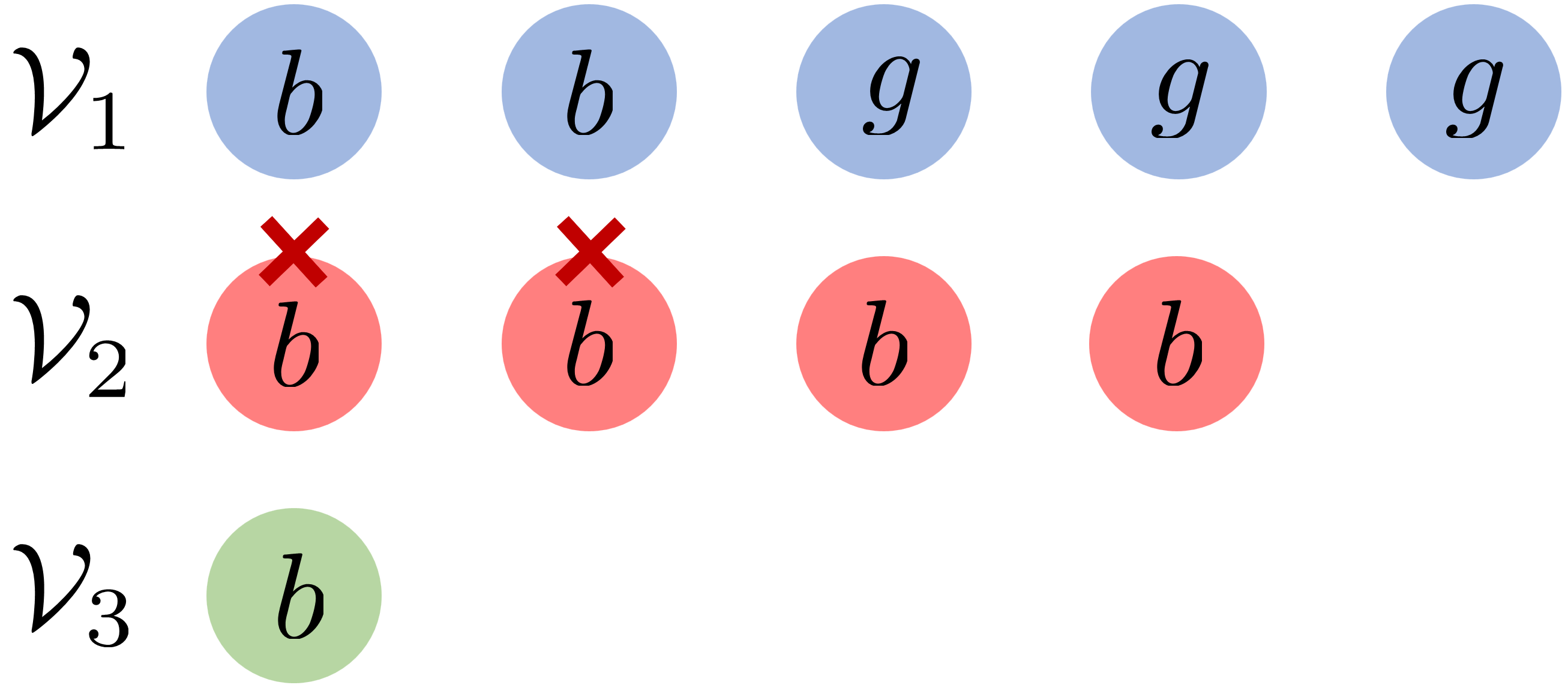
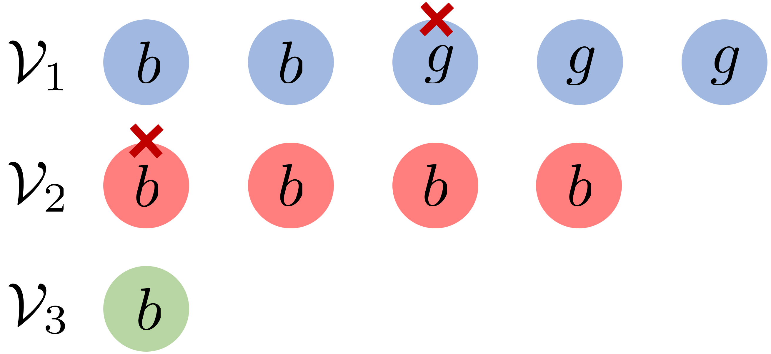
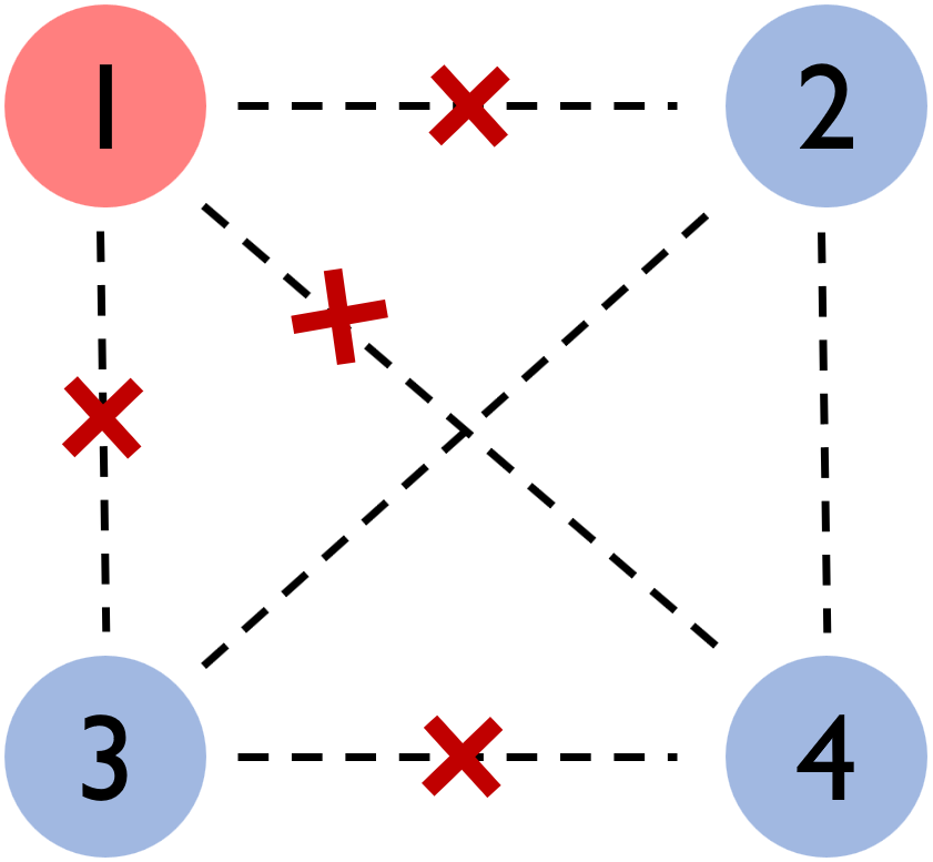
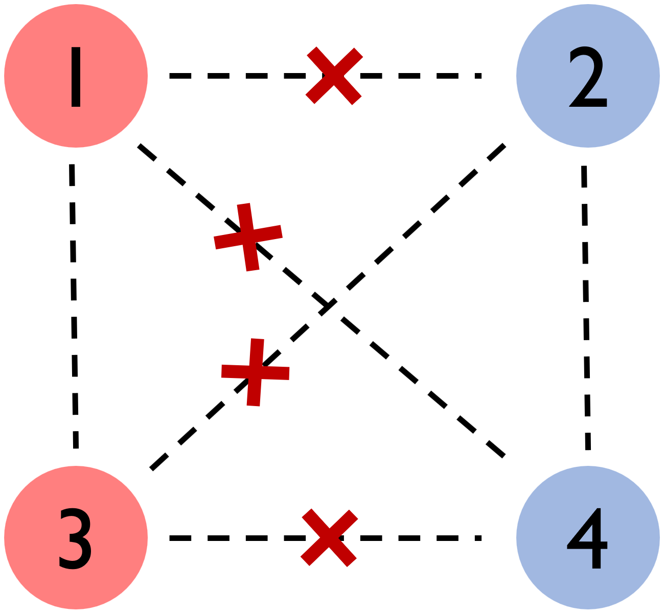
The communication attack cuts off the communication links among robots and thus disables the sharing of sensor measurements. With communication attacks, the robot team may be partitioned into several isolated subgroups (i.e., no communication is available between them, see subgroups {1} and {2,3,4} in Fig. 2-(a)). Within each subgroup, the robots are connected (not necessarily fully connected, see subgroup {2,3,4} in Fig. 2-(a)), and they can share sensor measurements to collectively estimate the states of targets. However, the isolated subgroups cannot utilize the sensor measurements from each other, and thus they update the estimate of the targets’ states by EKF individually. In this case, the team’s tracking quality is set as the tracking quality of the subgroup that performs the best.
Refer to caption
Refer to caption
Figure 2: A team of 444 robots (disks) encounters 444 communication attacks (red crosses). In subfigure (a), the communication attacks cut off 444 communication links (dashed lines) and partition the robot team into 222 isolated subgroups {1} and {2,3,4}. Thus, the number of robots in the largest subgroup nmax=3subscript𝑛3n_{\max}=3. The subgroup {1} and {2,3,4} cannot share sensing measurements. The robots in subgroup {2,3,4} can share measurements even though they are not fully connected due to the communication attack between robot 3 and robot 4. In subfigure (b), the 444 communication attacks partition the robot team into 222 isolated subgroups (red and blue subgroups, each with two robots), and thus nmax=2subscript𝑛2n_{\max}=2. Since at most 222 robots can communicate (in subfigure (a), at most 333 robots can communicate), it is more likely the 444 communication attacks in subfigure (b) are worse for the robot team.

We assume the maximum numbers of sensing and communication attacks/failures at each time step are known, denoted by αssubscript𝛼𝑠\alpha_{s} and αcsubscript𝛼𝑐\alpha_{c}, respectively. We also assume the attacks at a time step to be effective in this specific time step only. That is, the sensing or communication links attacked at time step t𝑡t may be active at another time step tsuperscript𝑡t^{\prime}. Also, if a robot encounters sensing attack only, it can still act as information relay node to communicate with other robots to help them share sensor measurements.

II-B Problem Definition

We next formally define the main problem in this paper.

Problem 1 (Robust Multi-Robot Active Target Tracking).

In reference to the framework in Section II-A, consider, a set of mobile robots 𝒱𝒱\mathcal{V}, with the motion model eq. (1), and with sensing and communication capabilities (Section II-A, c) & d)); additionally, consider a set of targets 𝒯𝒯\mathcal{T} with motion model eq. (2); furthermore, consider a multi-target tracking objective function ΦΦ\Phi (Section II-A, e)); finally, consider the maximum numbers of sensing and communication attacks/failures, αssubscript𝛼𝑠\alpha_{s} and αcsubscript𝛼𝑐\alpha_{c}. For all robots i𝒱𝑖𝒱i\in\mathcal{V}, find the control inputs 𝐮𝐭subscript𝐮𝐭{\mathbf{u_{t}}} at the current time step t𝑡t to maximize the tracking objective ΦΦ\Phi against the worst-case sensing attacks that remove the measurements from (at most) αssubscript𝛼𝑠\alpha_{s} robots and against the worst-case communication attacks that block (at most) αcsubscript𝛼𝑐\alpha_{c} communication links among robots at the next time step t+1𝑡1t+1. Formally:

max𝐮𝒱,t𝒰𝒱min𝒜s𝒱,𝒜cΦ(𝒱𝒜s,𝒜c)s.t.|𝒜s|αs,αsN,|𝒜c|αc,αcN(N1)2,formulae-sequencesubscriptsubscript𝐮𝒱𝑡subscript𝒰𝒱subscriptformulae-sequencesubscript𝒜𝑠𝒱subscript𝒜𝑐Φ𝒱subscript𝒜𝑠subscript𝒜𝑐s.t.subscript𝒜𝑠subscript𝛼𝑠formulae-sequencesubscript𝛼𝑠𝑁formulae-sequencesubscript𝒜𝑐subscript𝛼𝑐subscript𝛼𝑐𝑁𝑁12\displaystyle\begin{split}&\max_{{\mathbf{u}}_{{\mathcal{V}},t}\;\in\;{\mathcal{U}}_{{\mathcal{V}}}}\;\min_{{\mathcal{A}}_{s}\;\subseteq\;{\mathcal{V}},\;{\mathcal{A}}_{c}\;\subseteq\;{\mathcal{E}}}\Phi({\mathcal{V}}\setminus{\mathcal{A}}_{s},{\mathcal{E}}\setminus{\mathcal{A}}_{c})\\ &{\text{s.t.}}\;\;~{}|{\mathcal{A}}_{s}|\leq\alpha_{s},~{}\alpha_{s}\leq N,\\ &\hskip 21.33955pt|{\mathcal{A}}_{c}|\leq\alpha_{c},~{}\alpha_{c}\leq\frac{N(N-1)}{2},\end{split} (4)

where 𝒰𝒱i𝒱𝒰isubscript𝒰𝒱subscript𝑖𝒱subscript𝒰𝑖{\mathcal{U}}_{{\mathcal{V}}}\triangleq\bigcup_{i\in{\mathcal{V}}}{\mathcal{U}}_{i} denotes the joint set of available control inputs of all robots; 𝒜ssubscript𝒜𝑠{\mathcal{A}}_{s} and 𝒜csubscript𝒜𝑐{\mathcal{A}}_{c} denote the set of robots with sensing removals and the set of communication links (edges) blocked; Φ(𝒱𝒜s,𝒜c)Φ𝒱subscript𝒜𝑠subscript𝒜𝑐\Phi({\mathcal{V}}\setminus{\mathcal{A}}_{s},{\mathcal{E}}\setminus{\mathcal{A}}_{c}) is the team’s tracking quality with the robots’ control input 𝐮𝒱,tsubscript𝐮𝒱𝑡{\mathbf{u}}_{{\mathcal{V}},t} and the sensing and communication attack sets, 𝒜ssubscript𝒜𝑠{\mathcal{A}}_{s} and 𝒜csubscript𝒜𝑐{\mathcal{A}}_{c}.

Problem 1 captures a two-stage sequential game with perfect information between two players [25, Chapter 4], namely, the robots (who aim to optimize the team’s target tracking quality) and the attacker (who aims to undermine the target tracking quality). The robots play first by selecting the control input 𝐮𝒱,tsubscript𝐮𝒱𝑡{\mathbf{u}}_{\mathcal{V},t} at time step t𝑡t to move to the state 𝐱t+1:=[𝐱1,t+1;𝐱2,t+1;;𝐱N,t+1]assignsubscript𝐱𝑡1subscript𝐱1𝑡1subscript𝐱2𝑡1subscript𝐱𝑁𝑡1{\mathbf{x}}_{t+1}:=[{\mathbf{x}}_{1,t+1};{\mathbf{x}}_{2,t+1};\cdots;{\mathbf{x}}_{N,t+1}] at the next time step t+1𝑡1t+1 (by eq. (1)). After observing 𝐱t+1subscript𝐱𝑡1{\mathbf{x}}_{t+1}, the attacker responds with the worst-case sensing and communication removals (𝒜s,𝒜c)subscript𝒜𝑠subscript𝒜𝑐({\mathcal{A}}_{s},{\mathcal{A}}_{c}).

Problem 1 goes beyond the classical objective (e.g., the attacking sets 𝒜s,𝒜c=subscript𝒜𝑠subscript𝒜𝑐{\mathcal{A}}_{s},{\mathcal{A}}_{c}=\emptyset) of multi-robot target tracking, by securing the team performance against worst-case sensing and communication attacks/failures.

III Algorithm for Problem 1

We present the first scalable algorithm (Algorithm 1), named Robust Active Target Tracking (RATT) for Problem 1. RATT sequentially executes two main steps—communication attack approximation (RATT’s line 1) and robust maximization against sensing attacks (RATT’s lines 2-15). In the first step, RATT utilizes a subroutine (Algorithm 2, named CAA) to approximate the number of the communication attacks αcsubscript𝛼𝑐\alpha_{c} to a certain number of sensing attacks αc,ssubscript𝛼𝑐𝑠\alpha_{c,s}. In the second step, RATT capitalizes on the algorithm results in [15, 19] to maximize the team’s tracking quality against the total number of sensing attacks (i.e., the original number of sensing attacks αssubscript𝛼𝑠\alpha_{s} and the approximated number of sensing attacks αc,ssubscript𝛼𝑐𝑠\alpha_{c,s}). We describe RATT’s two steps in more detail below.

0:  Current time step t𝑡t; set of N𝑁N robots 𝒱𝒱{\mathcal{V}}; each robot i𝑖i’s dynamics fisubscript𝑓𝑖f_{i} including current state 𝐱i,tsubscript𝐱𝑖𝑡{\mathbf{x}}_{i,t}; each robot i𝑖i’s available control inputs 𝒰isubscript𝒰𝑖\mathcal{U}_{i}; set of M𝑀M targets 𝒯𝒯{\mathcal{T}}; each target j𝑗j’s dynamics including state transition matrix 𝐀jsubscript𝐀𝑗{\mathbf{A}}_{j}, current covariance 𝐐j,tsubscript𝐐𝑗𝑡{\mathbf{Q}}_{j,t} of the motion noise, current state estimate 𝐲^j,tsubscript^𝐲𝑗𝑡\hat{{\mathbf{y}}}_{j,t}, and current covariance estimate 𝚺j,tsubscript𝚺𝑗𝑡{\mathbf{\Sigma}}_{j,t}; measurement model of each robot i𝑖i to each target j𝑗j including current measurement matrix 𝐇i,tjsuperscriptsubscript𝐇𝑖𝑡𝑗{\mathbf{H}}_{i,t}^{j} and current covariance 𝐑(𝐱i,t,𝐲j,t)𝐑subscript𝐱𝑖𝑡subscript𝐲𝑗𝑡{\mathbf{R}}({\mathbf{x}}_{i,t},{\mathbf{y}}_{j,t}) of the measurement noise; team’s target tracking objective function ΦΦ\Phi; number of sensing attacks αssubscript𝛼𝑠\alpha_{s}; number of communication attacks αcsubscript𝛼𝑐\alpha_{c}.
0:  Control inputs 𝐮i,tsubscript𝐮𝑖𝑡{\mathbf{u}}_{i,t} for all robots i𝒱𝑖𝒱i\in{\mathcal{V}}.
1:  Compute αc,ssubscript𝛼𝑐𝑠\alpha_{c,s} by calling CAA(N,αc)CAA𝑁subscript𝛼𝑐\texttt{CAA}(N,\alpha_{c});
2:  Set α:=αs+αc,sassign𝛼subscript𝛼𝑠subscript𝛼𝑐𝑠\alpha:=\alpha_{s}+\alpha_{c,s};
3:  if α<N𝛼𝑁\alpha<N then
4:     for i𝒱𝑖𝒱i\in{\mathcal{V}} do
5:        Φ{i},0max𝐮i,t𝒰iΦ({i})subscriptsuperscriptΦ𝑖0subscript𝐮𝑖𝑡subscript𝒰𝑖Φ𝑖\Phi^{\star}_{\{i\},0}\triangleq\underset{{\mathbf{u}}_{i,t}~{}\in~{}{\mathcal{U}}_{i}}{\max}\;\Phi(\{i\}\setminus\emptyset);
6:     Sort out a subset 𝒱bsubscript𝒱𝑏{\mathcal{V}}_{b} of α𝛼\alpha robots, such that Φ{i},0Φ{i},0,i𝒱bformulae-sequencesubscriptsuperscriptΦ𝑖0subscriptsuperscriptΦsuperscript𝑖0for-all𝑖subscript𝒱𝑏\Phi^{\star}_{\{i\},0}\geq\Phi^{\star}_{\{i^{\prime}\},0},~{}\forall i\in{\mathcal{V}}_{b} and i𝒱𝒱bfor-allsuperscript𝑖𝒱subscript𝒱𝑏\forall i^{\prime}\in{\mathcal{V}}\setminus{\mathcal{V}}_{b};
7:     for i𝒱b𝑖subscript𝒱𝑏i\in{\mathcal{V}}_{b} do
8:        𝐮i,t=argmax𝐮i,t𝒰iΦ({i})subscript𝐮𝑖𝑡argsubscript𝐮𝑖𝑡subscript𝒰𝑖Φ𝑖{\mathbf{u}}_{i,t}=\text{arg}\underset{{\mathbf{u}}_{i,t}~{}\in~{}{\mathcal{U}}_{i}}{\max}\Phi(\{i\}\setminus\emptyset);
9:     𝒱gsubscript𝒱𝑔{\mathcal{V}}_{g}\leftarrow\emptyset;
10:     while 𝒱(𝒱b𝒱g)𝒱subscript𝒱𝑏subscript𝒱𝑔{\mathcal{V}}\setminus({\mathcal{V}}_{b}\cup{\mathcal{V}}_{g})\neq\emptyset do
11:        Find robot i𝒱(𝒱b𝒱g)superscript𝑖𝒱subscript𝒱𝑏subscript𝒱𝑔i^{\prime}\in{\mathcal{V}}\setminus({\mathcal{V}}_{b}\cup{\mathcal{V}}_{g}) and its control input 𝐮i,tsubscript𝐮superscript𝑖𝑡{\mathbf{u}}_{i^{\prime},t} such that 𝐮i,targmax𝐮v,t𝒰𝒱(𝒱b𝒱g)Φ((𝒱g{v}))subscript𝐮superscript𝑖𝑡argsubscript𝐮𝑣𝑡subscript𝒰𝒱subscript𝒱𝑏subscript𝒱𝑔Φsubscript𝒱𝑔𝑣{\mathbf{u}}_{i^{\prime},t}\in\text{arg}\underset{{\mathbf{u}}_{v,t}~{}\in~{}{\mathcal{U}}_{{\mathcal{V}}\setminus({\mathcal{V}}_{b}\cup{\mathcal{V}}_{g})}}{\max}\Phi(({\mathcal{V}}_{g}\cup\{v\})\setminus\emptyset)
                                           Φ(𝒱g)Φsubscript𝒱𝑔-\Phi({\mathcal{V}}_{g}\setminus\emptyset);
12:        𝒱g𝒱g{i}subscript𝒱𝑔subscript𝒱𝑔superscript𝑖{\mathcal{V}}_{g}\leftarrow{\mathcal{V}}_{g}\cup\{i^{\prime}\};
13:  else
14:     for i𝒱𝑖𝒱i\in{\mathcal{V}} do
15:        𝐮i,t=argmax𝐮i,t𝒰iΦ({i})subscript𝐮𝑖𝑡argsubscript𝐮𝑖𝑡subscript𝒰𝑖Φ𝑖{\mathbf{u}}_{i,t}=\text{arg}\underset{{\mathbf{u}}_{i,t}~{}\in~{}{\mathcal{U}}_{i}}{\max}\Phi(\{i\}\setminus\emptyset);
Algorithm 1 Robust Active Target Tracking (RATT).
0:  Number of robots N𝑁N in the team; number of worst-case communication attacks αcsubscript𝛼𝑐\alpha_{c}.
0:  Approximated number of sensing attacks αc,ssubscript𝛼𝑐𝑠\alpha_{c,s}.
1:  Initialize nmax=0subscript𝑛0n_{\max}=0;
2:  Compute er=N(N1)2αcsubscript𝑒𝑟𝑁𝑁12subscript𝛼𝑐e_{r}=\frac{N(N-1)}{2}-\alpha_{c};
3:  for each n[1,2,,N]𝑛12𝑁n\in[1,2,\cdots,N] do
4:     Compute qn=Nnsubscript𝑞𝑛𝑁𝑛q_{n}=\lfloor{\frac{N}{n}}\rfloor, rn=Nnqnsubscript𝑟𝑛𝑁𝑛subscript𝑞𝑛r_{n}=N-nq_{n}; and
e¯n=qnn(n1)2+rn(rn1)2subscript¯𝑒𝑛subscript𝑞𝑛𝑛𝑛12subscript𝑟𝑛subscript𝑟𝑛12\overline{e}_{n}=q_{n}\frac{n(n-1)}{2}+\frac{r_{n}(r_{n}-1)}{2};
5:     if ere¯nsubscript𝑒𝑟subscript¯𝑒𝑛e_{r}\leq\overline{e}_{n} then
6:        Set nmax=nsubscript𝑛𝑛n_{\max}=n, stop for loop;
7:  return αc,s=Nnmaxsubscript𝛼𝑐𝑠𝑁subscript𝑛\alpha_{c,s}=N-n_{\max}.
Algorithm 2 Communication Attack Approximation (CAA).

III-A Communication attack approximation (Step-1 of RATT)

We present the first step of RATT, communication attack approximation (RATT’s line 1, that calls CAA, with pseudo-code presented in Algorithm 2). CAA approximates the number of communication attacks to a certain number of sensing attacks for the robot team. The intuition behind CAA is from the equivalent consequence of communication attacks and sensing attacks. Recall that the sensing attack removes sensor measurements and the communication attack disables measurement sharing among isolated subgroups (Section II-A-(f)). Thus, if one subgroup cannot communicate with the other subgroups to utilize their sensor measurements, from the perspective of this specific subgroup, it is equivalent to the case that the communications are not attacked but the other subgroups encounter sensing attacks and lose their sensor measurements. For example, in Fig. 2-(a), the 444 communication attacks result in two isolated subgroups {2,3,4} and {1}, for subgroup {2,3,4}, it cannot utilize the sensor measurements from subgroup {1}, which can be seen as the scenario that subgroup {2,3,4} can communicate with subgroup {1} but the measurements of subgroup {1} are removed by sensing attacks. Thus, for subgroup {2,3,4}, these 444 communication attacks are equivalent to 111 sensing attack on robot 1. Likewise, for subgroup {1}, these 444 communication attacks are equivalent to 333 sensing attacks on robots 2, 3, 4. Therefore, for each subgroup, its approximated number of sensing attacks can be set as the number of robots in the other isolated subgroups.

Refer to caption
(a) e¯1=0subscript¯𝑒10\overline{e}_{1}=0, n=1𝑛1n=1
Refer to caption
(b) e¯2=2subscript¯𝑒22\overline{e}_{2}=2, n=2𝑛2n=2
Refer to caption
(c) e¯3=4subscript¯𝑒34\overline{e}_{3}=4, n=3𝑛3n=3
Refer to caption
(d) e¯4=6subscript¯𝑒46\overline{e}_{4}=6, n=4𝑛4n=4
Refer to caption
(e) e¯5=10subscript¯𝑒510\overline{e}_{5}=10, n=5𝑛5n=5
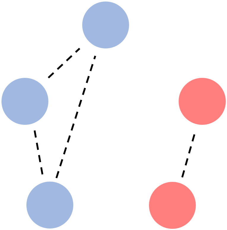
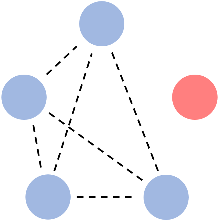
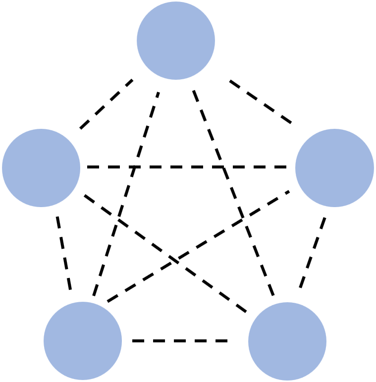
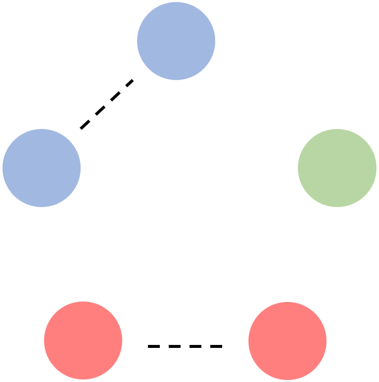
Figure 3: Qualitative description of CAA computing the maximal number of edges e¯n,n[1,2,,N]subscript¯𝑒𝑛𝑛12𝑁\overline{e}_{n},n\in[1,2,\cdots,N] for a team of five robots (N=5𝑁5N=5) by eq. (5). The disks represent the robots. The robots within the same subgroup have the same color. The dashed lines show the available edges between robots. Based on e¯nsubscript¯𝑒𝑛\overline{e}_{n}, the number of the robots in the largest subgroup nmaxsubscript𝑛n_{\max} and the approximated number of sensing attacks αc,ssubscript𝛼𝑐𝑠\alpha_{c,s} with any number of worst-case communication attacks αcsubscript𝛼𝑐\alpha_{c} can be computed. For example, when αc=7subscript𝛼𝑐7\alpha_{c}=7, one has the remaining number of edges er=N(N1)/2αc=107=3subscript𝑒𝑟𝑁𝑁12subscript𝛼𝑐1073e_{r}=N(N-1)/2-\alpha_{c}=10-7=3. Then CAA checks n[1,2,3,4,5]𝑛12345n\in[1,2,3,4,5] in ascending order, and stops at n=3𝑛3n=3 since ere¯3subscript𝑒𝑟subscript¯𝑒3e_{r}\leq\overline{e}_{3} holds for the first time. Thus, CAA sets nmax=3subscript𝑛3n_{\max}=3 and computes αc,s=Nnmax=2subscript𝛼𝑐𝑠𝑁subscript𝑛2\alpha_{c,s}=N-n_{\max}=2.

Notably, the approximated number of sensing attacks can be varying for different subgroups, which brings the problem of deciding the approximated number of sensing attacks for the entire robot team, denoted henceforth by αc,ssubscript𝛼𝑐𝑠\alpha_{c,s}. To address this issue, we focus on the largest subgroup (i.e., the subgroup with the most number of robots among all subgroups).111If there exist multiple largest subgroups, we can randomly pick one. That is because the team’s tracking quality equals the tracking quality of the subgroup that performs the best (Section II-A-(f)), and the subgroup with more robots is likely to perform better (since more measurements are available).222Notably, RATT does not require the assumption that the largest subgroup must perform better than the others for providing hard guarantees against worst-case communication attacks (Section IV-B). In other words, for computing the team’s tracking quality, it is more likely that the largest subgroup will be used and other smaller subgroups will be ignored. Therefore, αc,ssubscript𝛼𝑐𝑠\alpha_{c,s} can be conjectured as the approximated number of sensing attacks in the largest subgroup. Then, as mentioned above, αc,ssubscript𝛼𝑐𝑠\alpha_{c,s} can be computed as the number of robots that are in other smaller subgroups. We denote the number of robots in the largest subgroup as nmaxsubscript𝑛n_{\max}. Clearly, nmax+αc,s=Nsubscript𝑛subscript𝛼𝑐𝑠𝑁n_{\max}+\alpha_{c,s}=N. Then the critical point is to determine nmaxsubscript𝑛n_{\max} after αcsubscript𝛼𝑐\alpha_{c} worst-case communication attacks.

Also, since a smaller subgroup is more likely to perform worse than a larger subgroup, the worst-case communication attacks tend to separate the robot team evenly into more, smaller subgroups. In this way, the communication attacks are more presumably to compromise the coordination between the robots to the largest extent. More specifically, the worst-case communication attacks aim to make nmaxsubscript𝑛n_{\max} as small as possible. Considering the intent of the worst-case communication attacks, we present CAA (Algorithm 2) that efficiently computes nmaxsubscript𝑛n_{\max} and αc,ssubscript𝛼𝑐𝑠\alpha_{c,s} as follows:

  • CAA initializes the number of robots in the largest subgroup nmaxsubscript𝑛n_{\max} as zero (Algorithm 2, line 1).

  • CAA computes the number of the remaining (unattacked) edges (communication links) ersubscript𝑒𝑟e_{r} the robot team has after αcsubscript𝛼𝑐\alpha_{c} communication attacks (Algorithm 2, line 2).

  • CAA determines nmaxsubscript𝑛n_{\max} by iterating over all possible candidates n[1,2,,N]𝑛12𝑁n\in[1,2,\cdots,N] in ascending order (Algorithm 2, lines 3-6). For each iteration (each n𝑛n),

    1. 1.

      CAA first computes the maximal number of available (unattacked) edges e¯nsubscript¯𝑒𝑛\overline{e}_{n} the robot team can have when the number of robots in the largest subgroup is n𝑛n (Algorithm 2, line 2, cf. Fig. 3). Specifically, it computes the number of the largest subgroups (each has n𝑛n robots) as

      qn=Nn,subscript𝑞𝑛𝑁𝑛q_{n}=\lfloor{\frac{N}{n}}\rfloor,

      the remaining robots in the smaller subgroup as

      rn=Nnqn,subscript𝑟𝑛𝑁𝑛subscript𝑞𝑛r_{n}=N-nq_{n},

      and e¯nsubscript¯𝑒𝑛\overline{e}_{n} as the total number of available edges in the largest subgroups and the smaller subgroup, i.e.,

      en=qnn(n1)2+rn(rn1)2.subscript𝑒𝑛subscript𝑞𝑛𝑛𝑛12subscript𝑟𝑛subscript𝑟𝑛12e_{n}=q_{n}\frac{n(n-1)}{2}+\frac{r_{n}(r_{n}-1)}{2}. (5)
    2. 2.

      CAA then compares the number of the remaining edges ersubscript𝑒𝑟e_{r} with e¯nsubscript¯𝑒𝑛\overline{e}_{n}. If ersubscript𝑒𝑟e_{r} is less than or equal to e¯nsubscript¯𝑒𝑛\overline{e}_{n} (Algorithm 2, line 5), CAA sets nmaxsubscript𝑛n_{\max} as n𝑛n and stops the loop (Algorithm 2, line 6) to make sure that ere¯nsubscript𝑒𝑟subscript¯𝑒𝑛e_{r}\leq\overline{e}_{n} holds for the first time.444Notably, by definition of e¯nsubscript¯𝑒𝑛\overline{e}_{n}, a larger n𝑛n gives a larger e¯nsubscript¯𝑒𝑛\overline{e}_{n}. Thus, if ere¯nsubscript𝑒𝑟subscript¯𝑒𝑛e_{r}\leq\overline{e}_{n} holds, ere¯nsubscript𝑒𝑟subscript¯𝑒superscript𝑛e_{r}\leq\overline{e}_{n^{\prime}} also holds with any n>nsuperscript𝑛𝑛n^{\prime}>n.

  • With nmaxsubscript𝑛n_{\max} obtained, CAA computes the approximated number of sensing attacks αc,ssubscript𝛼𝑐𝑠\alpha_{c,s} as Nnmax𝑁subscript𝑛N-n_{\max}.

An illustrative example of how CAA computes e¯nsubscript¯𝑒𝑛\overline{e}_{n}, nmaxsubscript𝑛n_{\max}, and αc,ssubscript𝛼𝑐𝑠\alpha_{c,s} is shown in Fig. 3.

III-B Robust maximization against sensing attacks (Step-2 of RATT

We now present the second step of RATT: robust maximization against total sensing attacks (RATT’s lines 2-15). This step follows the traits of the robust algorithm in [15, 19], which applies a two-step procedure to select robust actions for the robots against a fixed number of attacks (e.g., αsuperscript𝛼\alpha^{\prime}). We recall here the two steps of the robust algorithm. First, it tries to conjecture the worst-case αsuperscript𝛼\alpha^{\prime} attacks to the robots, and toward this end, builds a bait action set to attract these attacks. Particularly, the bait set contains the top αsuperscript𝛼\alpha^{\prime} individual actions that contribute the most to the team performance from αsuperscript𝛼\alpha^{\prime} robots. In the second step, the robust algorithm greedily selects actions for the remaining Nα𝑁superscript𝛼N-\alpha^{\prime} robots by the standard greedy algorithm [22, Section 2]. On this basis, RATT’s second step is as follows:

  • RATT computes the total number of sensing attacks α𝛼\alpha as the summation of the original number of sensing attacks αssubscript𝛼𝑠\alpha_{s} and the approximated number of sensing attacked αc,ssubscript𝛼𝑐𝑠\alpha_{c,s} (Algorithm 1, line 2).

  • If the total number of sensing attacks α𝛼\alpha is less than the number of robots N𝑁N (Algorithm 1, line 3), RATT follows a two-step process, similar to the robust algorithm [15, 19], to choose robots’ control inputs against the total α𝛼\alpha sensing attacks.

    1. 1.

      First, RATT selects the bait control inputs for α𝛼\alpha robots to attract the total α𝛼\alpha sensing attacks (Algorithm 1, lines 4-8). Specifically, it first computes the maximum individual tracking quality Φ{i},0subscriptsuperscriptΦ𝑖0\Phi^{\star}_{\{i\},0}555In Algorithm 1, the number of communication attacks is approximated by a certain number of sensing attacks. Thus, for clarify, we omit here the dependence of tracking quality ΦΦ\Phi on the communication links {\mathcal{E}}. that each robot i𝑖i can attain by executing one of its control inputs, assuming no attacks (Algorithm 1, lines 4-5). It then finds the top α𝛼\alpha robots 𝒱bsubscript𝒱𝑏{\mathcal{V}}_{b} whose maximum individual tracking qualities are among the top α𝛼\alpha ones (Algorithm 1, line 6). Finally, for each robot in 𝒱bsubscript𝒱𝑏{\mathcal{V}}_{b}, RATT decides its control input as the one that achieves its maximum individual tracking quality (Algorithm 1, line 8).

    2. 2.

      Second, RATT greedily selects control inputs for the rest of the Nα𝑁𝛼N-\alpha robots 𝒱𝒱b𝒱subscript𝒱𝑏{\mathcal{V}}\setminus{\mathcal{V}}_{b} by following the standard greedy algorithm [22, Section 2] (Algorithm 1, lines 9-12). Particularly, at each round, it finds a robot i𝒱𝒱bsuperscript𝑖𝒱subscript𝒱𝑏i^{\prime}\in{\mathcal{V}}\setminus{\mathcal{V}}_{b} and selects for it a control input which provides the maximum marginal gain in the joint tracking quality (Algorithm 1, line 1).

  • Instead, if the total number of sensing attacks α𝛼\alpha is larger than or equal to the number of robots N𝑁N666This could happen since the approximated number of sensing attacks αc,ssubscript𝛼𝑐𝑠\alpha_{c,s} can be larger than Nαs𝑁subscript𝛼𝑠N-\alpha_{s} when the number of communication attacks αcsubscript𝛼𝑐\alpha_{c} is large enough. (Algorithm 1, lines 13), RATT conjectures all the robots’ sensing will be attacked. To this end, it lets each robot do its individual best; i.e., it chooses for each robot the control input that achieves the maximum individual tracking quality (Algorithm 1, lines 14-15).

All in all, RATT decides the control inputs for all robots by sequentially executing CAA and the robust maximization. In addition, RATT is valid for any number of sensing and communication attacks.

IV Performance Analysis of Algorithm 1

In this section, we quantify RATT’s performance, by bounding its approximation performance and running time. To this end, we treat objective function ΦΦ\Phi as a set function (i.e., defined on the set of robots) and leverage the properties of set functions such as monotonicity, submodularity, and curvatures. We start with reviewing these useful properties and then analyze the performance of RATT.

IV-A Properties of Set Functions

Normalized set function [26]: Consider a finite, discrete set 𝒳𝒳{\mathcal{X}}, a set function ϕ:2𝒳:italic-ϕmaps-tosuperscript2𝒳\phi:2^{\mathcal{X}}\mapsto\mathbb{R} is normalized if ϕ()=0italic-ϕ0\phi(\emptyset)=0.

Non-negative set function [26]: Consider a finite, discrete set 𝒳𝒳{\mathcal{X}}, a set function ϕ:2𝒳:italic-ϕmaps-tosuperscript2𝒳\phi:2^{\mathcal{X}}\mapsto\mathbb{R} is non-negative if ϕ(𝒴)0italic-ϕ𝒴0\phi({\mathcal{Y}})\geq 0 for all 𝒴𝒳𝒴𝒳{\mathcal{Y}}\subseteq{\mathcal{X}}.

Non-decreasing set function [26]: Consider a finite, discrete set 𝒳𝒳{\mathcal{X}}, a set function ϕ:2𝒳:italic-ϕmaps-tosuperscript2𝒳\phi:2^{\mathcal{X}}\mapsto\mathbb{R} is non-decreasing if for any sets 𝒴𝒴𝒳𝒴superscript𝒴𝒳{\mathcal{Y}}\subseteq{\mathcal{Y}}^{\prime}\subseteq\mathcal{X}, ϕ(𝒴)ϕ(𝒴)italic-ϕ𝒴italic-ϕsuperscript𝒴\phi({\mathcal{Y}})\leq\phi({\mathcal{Y}}^{\prime}).

Modularity [26]: Consider a finite, discrete set 𝒳𝒳{\mathcal{X}}, a set function ϕ:2𝒳:italic-ϕmaps-tosuperscript2𝒳\phi:2^{\mathcal{X}}\mapsto\mathbb{R} is modular if ϕ(𝒴)=y𝒴italic-ϕ𝒴subscript𝑦𝒴\phi({\mathcal{Y}})=\sum_{y\in{\mathcal{Y}}} for all 𝒴𝒳𝒴𝒳{\mathcal{Y}}\subseteq{\mathcal{X}}.

That is, for a modular function ϕitalic-ϕ\phi, the contributions of 𝒳𝒳{\mathcal{X}}’s elements to function ϕitalic-ϕ\phi are additive. Hence, modularity also implies ϕ({x}𝒴)ϕ(𝒴)=ϕ(x)italic-ϕ𝑥𝒴italic-ϕ𝒴italic-ϕ𝑥\phi(\{x\}\cup{\mathcal{Y}})-\phi({\mathcal{Y}})=\phi(x) for all 𝒴𝒳𝒴𝒳{\mathcal{Y}}\subseteq{\mathcal{X}} and x𝒳𝒴𝑥𝒳𝒴x\in{\mathcal{X}}\setminus{\mathcal{Y}}.

Submodularity [26, Proposition 2.1]: Consider a finite ground set 𝒳𝒳{\mathcal{X}}, a set function ϕ:2𝒳:italic-ϕmaps-tosuperscript2𝒳\phi:2^{\mathcal{X}}\mapsto\mathbb{R} is submodular if ϕ(𝒴{x})ϕ(𝒴)ϕ(𝒴{x})ϕ(𝒴)italic-ϕ𝒴𝑥italic-ϕ𝒴italic-ϕsuperscript𝒴𝑥italic-ϕsuperscript𝒴\phi({\mathcal{Y}}\cup\{x\})-\phi({\mathcal{Y}})\geq\phi({\mathcal{Y}}^{\prime}\cup\{x\})-\phi({\mathcal{Y}}^{\prime}) for all 𝒴𝒴𝒳𝒴superscript𝒴𝒳{\mathcal{Y}}\subseteq{\mathcal{Y}}^{\prime}\subseteq\mathcal{X} and x𝒳𝑥𝒳x\in\mathcal{X}.

Hence, if ϕitalic-ϕ\phi is submodular, the marginal contribution ϕ(𝒴{x})ϕ(𝒴)italic-ϕ𝒴𝑥italic-ϕ𝒴\phi({\mathcal{Y}}\cup\{x\})-\phi({\mathcal{Y}}) diminishes as 𝒴𝒴{\mathcal{Y}} grows, for all x𝒳𝑥𝒳x\in{\mathcal{X}}. For a submodular function ϕitalic-ϕ\phi, the contributions of 𝒳𝒳{\mathcal{X}}’s elements to function ϕitalic-ϕ\phi is subadditive, contrary to ϕitalic-ϕ\phi being modular. Specifically, consider, without loss of generality, ϕitalic-ϕ\phi to be non-negative, then submodularity implies ϕ({x}𝒴)ϕ(𝒴)ϕ(x)italic-ϕ𝑥𝒴italic-ϕ𝒴italic-ϕ𝑥\phi(\{x\}\cup{\mathcal{Y}})-\phi({\mathcal{Y}})\leq\phi(x). Therefore, x𝑥x’s contribution to ϕitalic-ϕ\phi diminishes in the presence of 𝒴𝒴{\mathcal{Y}}.

Curvature [20]: Consider a finite, discrete set 𝒱𝒱{\mathcal{V}}, and a non-decreasing submodular function ϕ:2𝒳:italic-ϕmaps-tosuperscript2𝒳\phi:2^{\mathcal{X}}\mapsto\mathbb{R} such that, without loss of generality, ϕ(x)0italic-ϕ𝑥0\phi({x})\neq 0, for all x𝒳𝑥𝒳x\in\mathcal{X}. Then, ϕitalic-ϕ\phi’s curvature is defined as

kϕ1minx𝒳ϕ(𝒳)ϕ(𝒳{x})ϕ(x).subscript𝑘italic-ϕ1subscript𝑥𝒳italic-ϕ𝒳italic-ϕ𝒳𝑥italic-ϕ𝑥k_{\phi}\triangleq 1-\min_{x\in\mathcal{X}}\frac{\phi(\mathcal{X})-\phi(\mathcal{X}\setminus\{x\})}{\phi({x})}. (6)

The definition of curvature implies kϕ[0,1]subscript𝑘italic-ϕ01k_{\phi}\in[0,1]. Particularly, if kϕ=0subscript𝑘italic-ϕ0k_{\phi}=0, then ϕ(𝒳)ϕ(𝒳{x})=ϕ(x)italic-ϕ𝒳italic-ϕ𝒳𝑥italic-ϕ𝑥\phi(\mathcal{X})-\phi(\mathcal{X}\setminus\{x\})=\phi(x), for all x𝒱𝑥𝒱x\in{\mathcal{V}} (i.e., ϕitalic-ϕ\phi is modular). On the other hand, if kϕ=1subscript𝑘italic-ϕ1k_{\phi}=1, then there exist x𝒳𝑥𝒳x\in\mathcal{X} such that ϕ(𝒳)ϕ(𝒳{x})=0italic-ϕ𝒳italic-ϕ𝒳𝑥0\phi(\mathcal{X})-\phi(\mathcal{X}\setminus\{x\})=0 (i.e., x𝑥x has no additional contribution in the presence of 𝒳{x}𝒳𝑥\mathcal{X}\setminus\{x\}). Therefore, the curvature kϕsubscript𝑘italic-ϕk_{\phi} measures how far ϕitalic-ϕ\phi is from modularity: a smaller kϕsubscript𝑘italic-ϕk_{\phi} means ϕitalic-ϕ\phi is closer to being modular and a larger kϕsubscript𝑘italic-ϕk_{\phi} means ϕitalic-ϕ\phi is farther from being modular (i.e., is more submodular).

Total curvature [21, Section 8]: Consider a finite, discrete set 𝒳𝒳{\mathcal{X}}, and a non-decreasing set function ϕ:2𝒳:italic-ϕmaps-tosuperscript2𝒳\phi:2^{\mathcal{X}}\mapsto\mathbb{R}. Then, ϕitalic-ϕ\phi’s total curvature is defined as

cϕ1minx𝒳min𝒴,𝒴𝒳xϕ(𝒴{x})ϕ(𝒴)ϕ(𝒴{x})ϕ(𝒴).subscript𝑐italic-ϕ1subscript𝑥𝒳subscript𝒴superscript𝒴𝒳𝑥italic-ϕ𝒴𝑥italic-ϕ𝒴italic-ϕsuperscript𝒴𝑥italic-ϕsuperscript𝒴c_{\phi}\triangleq 1-\min_{x\in\mathcal{X}}\;\min_{{\mathcal{Y}},{\mathcal{Y^{\prime}}}\subseteq{\mathcal{X}}\setminus x}\;\frac{\phi(\mathcal{Y}\cup\{x\})-\phi(\mathcal{Y})}{\phi(\mathcal{Y^{\prime}}\cup\{x\})-\phi(\mathcal{Y^{\prime}})}. (7)

The definition of total curvature implies cϕ[0,1]subscript𝑐italic-ϕ01c_{\phi}\in[0,1]. Particularly, if cϕ=0subscript𝑐italic-ϕ0c_{\phi}=0, then ϕitalic-ϕ\phi is modular. Instead, if cϕ=1subscript𝑐italic-ϕ1c_{\phi}=1, then eq. (7) implies ϕitalic-ϕ\phi is non-decreasing, which is already assumed in the definition of total curvature. If ϕitalic-ϕ\phi is submodular, then total curvature becomes curvature, i.e., cϕ=kϕsubscript𝑐italic-ϕsubscript𝑘italic-ϕc_{\phi}=k_{\phi}.

IV-B Performance Analysis for RATT

We present RATT’s suboptimality bounds on its approximation performance and the upper bound on its running time. To this end, we use the following notations:

  • Φ𝒱,αs,,αcsuperscriptsubscriptΦ𝒱subscript𝛼𝑠subscript𝛼𝑐\Phi_{{\mathcal{V}},\alpha_{s},{\mathcal{E}},\alpha_{c}}^{\star} is the optimal value of Problem 1:

    Φ𝒱,αs,,αcmax𝐮𝒱,t𝒰𝒱min𝒜s𝒱,𝒜cΦ(𝒱𝒜s,𝒜c);superscriptsubscriptΦ𝒱subscript𝛼𝑠subscript𝛼𝑐subscriptsubscript𝐮𝒱𝑡subscript𝒰𝒱subscriptformulae-sequencesubscript𝒜𝑠𝒱subscript𝒜𝑐Φ𝒱subscript𝒜𝑠subscript𝒜𝑐\Phi_{{\mathcal{V}},\alpha_{s},{\mathcal{E}},\alpha_{c}}^{\star}\triangleq\\ \max_{{\mathbf{u}}_{{\mathcal{V}},t}\in{\mathcal{U}}_{{\mathcal{V}}}}\min_{{\mathcal{A}}_{s}\subseteq{\mathcal{V}},{\mathcal{A}}_{c}\subseteq{\mathcal{E}}}\Phi({\mathcal{V}}\setminus{\mathcal{A}}_{s},{\mathcal{E}}\setminus{\mathcal{A}}_{c});

    (𝒜s,𝒜c)superscriptsubscript𝒜𝑠superscriptsubscript𝒜𝑐(\mathcal{A}_{s}^{\star},\mathcal{A}_{c}^{\star}) is an optimal removal of the measurements from αssubscript𝛼𝑠\alpha_{s} robots and of αcsubscript𝛼𝑐\alpha_{c} communication links among N𝑁N robots per Problem 1:

    (𝒜s,𝒜c)argmin𝒜s𝒱,𝒜cΦ(𝒱𝒜s,𝒜c).superscriptsubscript𝒜𝑠superscriptsubscript𝒜𝑐argsubscriptformulae-sequencesubscript𝒜𝑠𝒱subscript𝒜𝑐Φ𝒱subscript𝒜𝑠subscript𝒜𝑐(\mathcal{A}_{s}^{\star},\mathcal{A}_{c}^{\star})\triangleq~{}\text{arg}\min_{{\mathcal{A}}_{s}\;\subseteq\;{\mathcal{V}},\;{\mathcal{A}}_{c}\;\subseteq\;{\mathcal{E}}}\Phi({\mathcal{V}}\setminus{\mathcal{A}}_{s},{\mathcal{E}}\setminus{\mathcal{A}}_{c}).
Theorem 1 (Approximation bound).

RATT returns control inputs 𝐮𝒱,tsubscript𝐮𝒱t{\mathbf{u}}_{{\mathcal{V}},t} such that

  1. 1.

    if Φ:2𝒱,:Φmaps-tosuperscript2𝒱\Phi:2^{{\mathcal{V}},{\mathcal{E}}}\mapsto\mathbb{R} is non-decreasing, and without loss of generality, normalized and non-negative, then

    Φ(𝒱𝒜s,𝒜c)Φ𝒱,αs,,αcmin[(1cΦ)3,(1cΦ)2αc,s];Φ𝒱superscriptsubscript𝒜𝑠superscriptsubscript𝒜𝑐superscriptsubscriptΦ𝒱subscript𝛼𝑠subscript𝛼𝑐superscript1subscript𝑐Φ3superscript1subscript𝑐Φ2subscript𝛼𝑐𝑠~{}\frac{\Phi({\mathcal{V}}\setminus{\mathcal{A}}_{s}^{\star},{\mathcal{E}}\setminus{\mathcal{A}}_{c}^{\star})}{\Phi_{{\mathcal{V}},\alpha_{s},{\mathcal{E}},\alpha_{c}}^{\star}}\geq\min[(1-c_{\Phi})^{3},\frac{(1-c_{\Phi})^{2}}{\alpha_{c,s}}]; (8)
  2. 2.

    if, additionally, ΦΦ\Phi is submodular, then

    Φ(𝒱𝒜s,𝒜c)Φ𝒱,αs,,αcmin[1kΦ1+kΦ,1kΦαc,s].Φ𝒱superscriptsubscript𝒜𝑠superscriptsubscript𝒜𝑐superscriptsubscriptΦ𝒱subscript𝛼𝑠subscript𝛼𝑐1subscript𝑘Φ1subscript𝑘Φ1subscript𝑘Φsubscript𝛼𝑐𝑠~{}\frac{\Phi({\mathcal{V}}\setminus{\mathcal{A}}_{s}^{\star},{\mathcal{E}}\setminus{\mathcal{A}}_{c}^{\star})}{\Phi_{{\mathcal{V}},\alpha_{s},{\mathcal{E}},\alpha_{c}}^{\star}}\geq\min[\frac{1-k_{\Phi}}{1+k_{\Phi}},\frac{1-k_{\Phi}}{\alpha_{c,s}}]. (9)
Theorem 2 (Running time).

RATT runs in O(|𝒰𝒱|2)Osuperscriptsubscript𝒰𝒱2O(|{\mathcal{U}}_{{\mathcal{V}}}|^{2}) time.

We provide the proofs for Theorem 1 and Theorem 2 in the appendix.

In Theorem 1, the approximation bounds in eqs. (8), (9) compare RATT’s selection 𝐮𝒱,tsubscript𝐮𝒱𝑡{\mathbf{u}}_{{\mathcal{V}},t} against an optimal selection of control inputs that attains the optimal value Φ𝒱,αs,,αcsuperscriptsubscriptΦ𝒱subscript𝛼𝑠subscript𝛼𝑐\Phi_{{\mathcal{V}},\alpha_{s},{\mathcal{E}},\alpha_{c}}^{\star} for Problem 1. In particular, eqs. (8), (9) imply that RATT guarantees a value for Problem 1 which can be near-optimal for 1) non-decreasing and 2) non-decreasing and submodular functions ΦΦ\Phi. For example, when cΦ<1subscript𝑐Φ1c_{\Phi}<1 or kΦ<1subscript𝑘Φ1k_{\Phi}<1, RATT’s selection is near-optimal in the sense that the approximation bounds are nonzero. Functions with cΦ<1subscript𝑐Φ1c_{\Phi}<1 include the mean square error (e.g., the trace of a Kalman filter’s covariance matrix) [27]; Functions with kΦ<1subscript𝑘Φ1k_{\Phi}<1 include logdet\log\det of positive-definite matrices (e.g., logdet\log\det of a Kalman filter’s covariance matrix) [24, 28]. In addition, when αc,s0subscript𝛼𝑐𝑠0\alpha_{c,s}\to 0 (e.g., no communication attacks αc0subscript𝛼𝑐0\alpha_{c}\to 0), the bound in eq. (8) becomes (1cΦ)3superscript1subscript𝑐Φ3(1-c_{\Phi})^{3} and bound in (9) becomes (1kΦ)/(1+kΦ)1subscript𝑘Φ1subscript𝑘Φ(1-k_{\Phi})/(1+k_{\Phi}), which parallels the results in [15, Theorem 1] and [19, Theorem 1] with sensing attacks only.

Furthermore, if αc,s0subscript𝛼𝑐𝑠0\alpha_{c,s}\to 0 and cΦ=0subscript𝑐Φ0c_{\Phi}=0 (or kΦ=0subscript𝑘Φ0k_{\Phi}=0), RATT becomes exact (i.e., the bounds in eqs. (8), (9) are 1). More broadly, the bound in eq. (8) increases as cΦsubscript𝑐Φc_{\Phi} decreases. Likewise, the bound in eq. (9) increases as kΦsubscript𝑘Φk_{\Phi} decreases. Hence, these curvature-depended bounds make a first step towards classifying the classes of 1) non-decreasing and 2) non-decreasing and submodular functions into the category for which Problem 1 can be approximated well (low curvature functions), and the category for which it cannot (high curvature functions). Notably, although it is known for the problem of set function maximization (without attacks) that the bound 1cΦ1subscript𝑐Φ1-c_{\Phi} is tight [21, Theorem 8.6], the tightness of (1cΦ)3superscript1subscript𝑐Φ3(1-c_{\Phi})^{3} in eq. (8) for Problem 1 is an open problem.

Theorem 2 implies that even though RATT goes beyond the objective of set function maximization without attacks or with sensing attacking only, its running time has the same order as that of state-of-the-art non-robust algorithms [22, 8] and robust algorithms against sensing attacks only [15, 19]. In particular, same as these algorithms, RATT terminates with O(|𝒰𝒱|2)𝑂superscriptsubscript𝒰𝒱2O(|{\mathcal{U}}_{{\mathcal{V}}}|^{2}) evaluations of the objective function ΦΦ\Phi.

Remark 1.

A myopic algorithm that selects bait control input for each robot independently of all other robots (in contrast to RATT, whose robust maximization step accounts for the control inputs of the other robots during the greedy selection), attains better approximation bounds. That is because, the myopic algorithm is the same as RATT when Nα𝑁𝛼N\leq\alpha and, in this instance, RATT achieves (1cΦ)2superscript1subscript𝑐Φ2(1-c_{\Phi})^{2} for non-decreasing functions and 1kΦ1subscript𝑘Φ1-k_{\Phi} for non-decreasing and submodular functions (cf. eqs. (69) and (95) in the appendix). However, being exclusively myopic, this algorithm has worse practical performance than that of the robust maximization (cf. [16, Remark 1]).
Refer to caption
(a) RATT without 1 sensing attack
Refer to caption
(b) NR-OPT without 1 sensing attack
Refer to caption
(c) RATT with 1 sensing attack
Refer to caption
(d) NR-OPT with 1 sensing attack
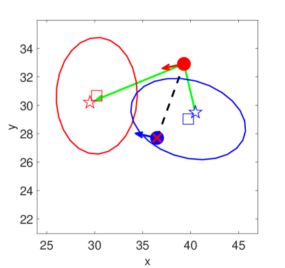
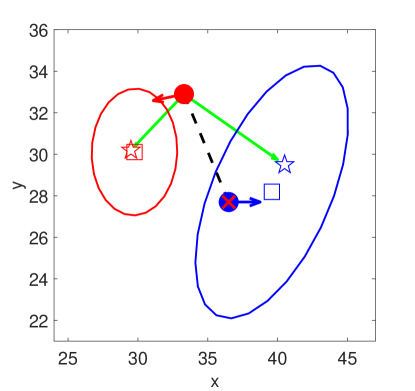
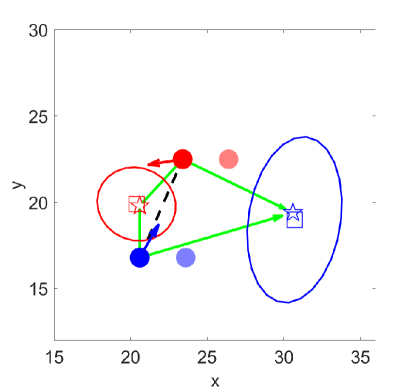
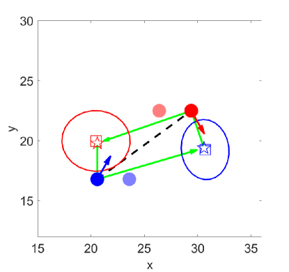
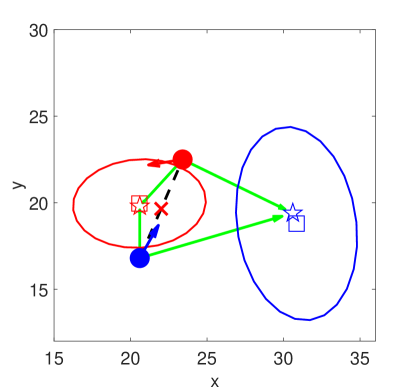
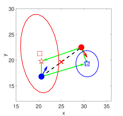
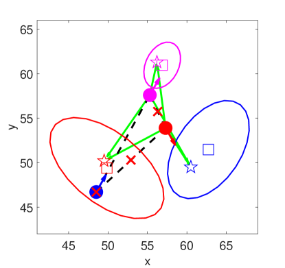
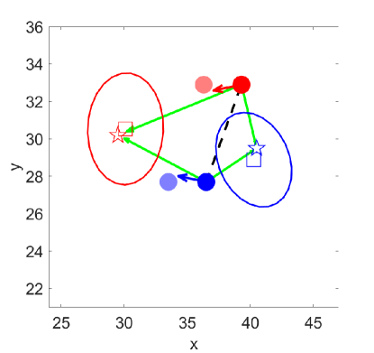
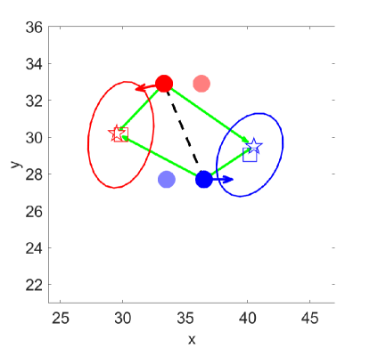
Figure 4: Comparison of 2 robots tracking 2 targets by RATT and NR-OPT without and with1 sensing attack. The transparent dot and the opaque dot represent the positions of the robot at the current time step and at one time step ahead, respectively. The arrow on the robot represents its heading. The pentagram, square, and ellipse indicate the true position, estimated mean position, and covariance of the target, respectively. The green arrow lines represent the sensing links from robots to targets. The black dashed line represents the communication link between robots. The red cross on a robot indicates the sensing attack on the robot.
Refer to caption
(a) RATT without 1 communication attack
Refer to caption
(b) NR-OPT without 1 communication attack
Refer to caption
(c) RATT with 1 communication attack
Refer to caption
(d) NR-OPT with 1 communication attack
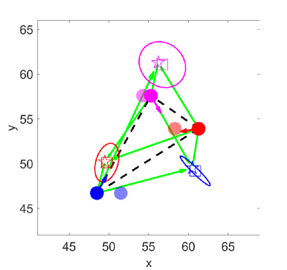
Figure 5: Comparison of 2 robots tracking 2 targets by RATT and NR-OPT without and with1 communication attack. The red cross on a communication link indicates the communication attack on the link. The representations of other depictions follows Fig. 4.
Refer to caption
(a) RATT without 1 sensing attack and 2 communication attacks
Refer to caption
(b) NR-OPT without 1 sensing attack and 2 communication attacks
Refer to caption
(c) RATT with 1 sensing attack and 2 communication attacks
Refer to caption
(d) NR-OPT with 1 sensing attack and 2 communication attacks
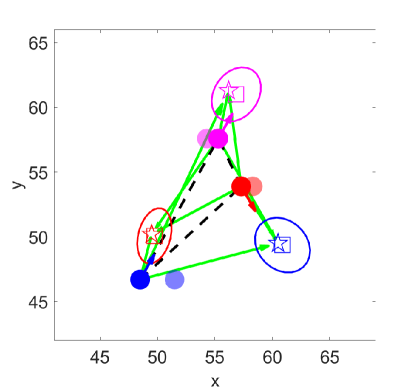
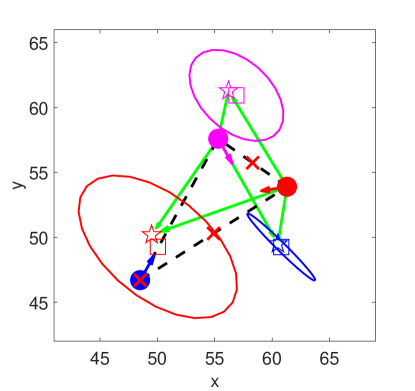
Figure 6: Comparison of 2 robots tracking 2 targets by RATT and NR-OPT without and with 1 sensing attack and 2 communication attacks. The representations of the depictions follows Fig. 4 and Fig. 5.

V Numerical Evaluations

We evaluate our algorithm (RATT, Algorithm 1) to demonstrate both the necessity for robust target tracking and the benefits of our approach. Particularly, the evaluations demonstrate: (i) RATT’s near-optimal performance, since it performs close to the exhaustive search approach for Problem 1 (which is viable in small-scale scenarios only); (ii) RATT is superior to non-robust heuristics against both worst-case and non-worst-case attacks. We perform the evaluations on a ThinkPad laptop with Intel Core i7 CPU @ 2.7 GHz and 64 GB RAM by using MATLAB 2020a on Ubuntu 20.04.

Compared algorithms. We compare RATT with four other algorithms. The algorithms differ in the way of selecting control inputs for the robots. The first algorithm is an optimal algorithm, which attains the optimal value for Problem 1 by exhaustively searching for all possible robots’ control inputs and all possible sensing and communication attacks. Evidently, this algorithm is only viable when the number of robots is small. We refer to this algorithm by OPT. The second algorithm is a non-robust optimal algorithm that ignores the possibility of attacks and uses the exhaustive search to choose control inputs to maximize the team performance (by assuming no attacks). Similar to OPT, this algorithm is viable for small-scale scenarios only. We refer to this algorithm by NR-OPT. The third algorithm is a (non-robust) greedy algorithm that also ignores the possibility of attacks and uses the standard greedy algorithm [22] to greedily select the control inputs. We refer to this algorithm by Greedy. The fourth algorithm is a random algorithm that selects randomly (uniformly) the control inputs. We refer to this algorithm by Random.

Comparison metrics. To access RATT’s effectiveness against sensing and communication attacks, we compare it with the other four algorithms across multiple scenarios, with varying numbers of robots N𝑁N, varying numbers of targets N𝑁N, and varying numbers of sensing and communication attacks, αssubscript𝛼𝑠\alpha_{s} and αcsubscript𝛼𝑐\alpha_{c}. We also test the algorithms’ performance against varying models of attacks such as the worst-case attack and bounded rational attack. In particular, we consider two performance metrics: the trace of the covariance matrix and the mean squared error (MSE, capturing the gap between the estimated position and true position), averaged over all the targets.

Experiment setup. In robust multi-target tracking, a team of mobile robots is tasked to track the locations of multiple moving targets, in the presence of a number of sensing and communication attacks. In what follows, we first specify the robot motion model, target motion model, sensor model, and tracking objective function, as introduced in Section II-A, and then specify the corresponding parameters.

Robot motion model

Each robot i𝒱𝑖𝒱i\in\mathcal{V} moves in a 2D environment with a unicycle motion model:

(xi,t+11xi,t+12θi,t+1)=(xi,t1xi,t2θi,t)+(νiτcos(θi,t)νiτsin(θi,t)τωi),matrixsuperscriptsubscript𝑥𝑖𝑡11superscriptsubscript𝑥𝑖𝑡12subscript𝜃𝑖𝑡1matrixsuperscriptsubscript𝑥𝑖𝑡1superscriptsubscript𝑥𝑖𝑡2subscript𝜃𝑖𝑡matrixsubscript𝜈𝑖𝜏subscript𝜃𝑖𝑡subscript𝜈𝑖𝜏subscript𝜃𝑖𝑡𝜏subscript𝜔𝑖\displaystyle\begin{split}{\begin{pmatrix}x_{i,t+1}^{1}\\ x_{i,t+1}^{2}\\ \theta_{i,t+1}\end{pmatrix}=\begin{pmatrix}x_{i,t}^{1}\\ x_{i,t}^{2}\\ \theta_{i,t}\end{pmatrix}+\begin{pmatrix}\nu_{i}\tau\cos(\theta_{i,t})\\ \nu_{i}\tau\sin(\theta_{i,t})\\ \tau\omega_{i}\end{pmatrix},}\end{split}

where 𝐱i=[xi1,xi2,θi]subscript𝐱𝑖superscriptsuperscriptsubscript𝑥𝑖1superscriptsubscript𝑥𝑖2subscript𝜃𝑖top{\mathbf{x}}_{i}=[x_{i}^{1},x_{i}^{2},\theta_{i}]^{\top} with [xi1,xi2]superscriptsuperscriptsubscript𝑥𝑖1superscriptsubscript𝑥𝑖2top[x_{i}^{1},x_{i}^{2}]^{\top} the position and θisubscript𝜃𝑖\theta_{i} the orientation of robot i𝑖i in the global frame. [νi,ωi]superscriptsubscript𝜈𝑖subscript𝜔𝑖top[\nu_{i},\omega_{i}]^{\top} denotes the control input (linear and angular velocities) of robot i𝑖i. τ𝜏\tau is the sampling period.

Target motion model

Each target i𝒯𝑖𝒯i\in\mathcal{T} moves in the 2D environment by following a circular motion model with additive white Gaussian noise:

(yj,t+11yj,t+12)=(yj,t1yj,t2)+(νjcos(τωj)νjsin(τωj))+𝐰j,t,matrixsuperscriptsubscript𝑦𝑗𝑡11superscriptsubscript𝑦𝑗𝑡12matrixsuperscriptsubscript𝑦𝑗𝑡1superscriptsubscript𝑦𝑗𝑡2matrixsubscript𝜈𝑗𝜏subscript𝜔𝑗subscript𝜈𝑗𝜏subscript𝜔𝑗subscript𝐰𝑗𝑡\displaystyle\begin{split}\begin{pmatrix}y_{j,t+1}^{1}\\ y_{j,t+1}^{2}\end{pmatrix}=\begin{pmatrix}y_{j,t}^{1}\\ y_{j,t}^{2}\end{pmatrix}+\begin{pmatrix}\nu_{j}\cos(\tau\omega_{j})\\ \nu_{j}\sin(\tau\omega_{j})\end{pmatrix}+{\mathbf{w}}_{j,t},\end{split}

where 𝐲i=[yj1,yj2]subscript𝐲𝑖superscriptsuperscriptsubscript𝑦𝑗1superscriptsubscript𝑦𝑗2top{\mathbf{y}}_{i}=[y_{j}^{1},y_{j}^{2}]^{\top} with [yj1,yj2]superscriptsuperscriptsubscript𝑦𝑗1superscriptsubscript𝑦𝑗2top[y_{j}^{1},y_{j}^{2}]^{\top} the position of target j𝑗j in the global frame. [νj,ωj]superscriptsubscript𝜈𝑗subscript𝜔𝑗top[\nu_{j},\omega_{j}]^{\top} denotes linear and angular velocities of target j𝑗j. The noise 𝐰j,t𝒩(0,𝐐)similar-tosubscript𝐰𝑗𝑡𝒩0𝐐{\mathbf{w}}_{j,t}\sim\mathcal{N}(0,{\mathbf{Q}}) with

𝐐=[σj200σj2].𝐐matrixsuperscriptsubscript𝜎𝑗200superscriptsubscript𝜎𝑗2{\mathbf{Q}}=\begin{bmatrix}\sigma_{j}^{2}&0\\ 0&\sigma_{j}^{2}\end{bmatrix}.
Sensor model

Each robot i𝑖i observes a target j𝑗j according to a range and bearing sensor model (as it is the case for depth camera):

hij(𝐱i,t,𝐲j,t)=[r(𝐱i,t,𝐲j,t)γ(𝐱i,t,𝐲j,t)]superscriptsubscript𝑖𝑗subscript𝐱𝑖𝑡subscript𝐲𝑗𝑡matrix𝑟subscript𝐱𝑖𝑡subscript𝐲𝑗𝑡𝛾subscript𝐱𝑖𝑡subscript𝐲𝑗𝑡\displaystyle h_{i}^{j}({\mathbf{x}}_{i,t},{\mathbf{y}}_{j,t})=\begin{bmatrix}r({\mathbf{x}}_{i,t},{\mathbf{y}}_{j,t})\\ \gamma({\mathbf{x}}_{i,t},{\mathbf{y}}_{j,t})\end{bmatrix}
[(yj,t2xi,t2)2+(yj,t1xi,t1)2atan2(yj,t2xi,t2,yj,t1xi,t1)θi,t]absentmatrixsuperscriptsuperscriptsubscript𝑦𝑗𝑡2superscriptsubscript𝑥𝑖𝑡22superscriptsuperscriptsubscript𝑦𝑗𝑡1superscriptsubscript𝑥𝑖𝑡12atan2superscriptsubscript𝑦𝑗𝑡2superscriptsubscript𝑥𝑖𝑡2superscriptsubscript𝑦𝑗𝑡1superscriptsubscript𝑥𝑖𝑡1subscript𝜃𝑖𝑡\displaystyle\triangleq\begin{bmatrix}\sqrt{(y_{j,t}^{2}-x_{i,t}^{2})^{2}+(y_{j,t}^{1}-x_{i,t}^{1})^{2}}\\ \text{atan2}(y_{j,t}^{2}-x_{i,t}^{2},y_{j,t}^{1}-x_{i,t}^{1})-\theta_{i,t}\end{bmatrix}

The measurement noise 𝐯i,tj(𝐱i,t,𝐲j,t)𝒩(0,𝐑(𝐱i,t,𝐲j,t))similar-tosuperscriptsubscript𝐯𝑖𝑡𝑗subscript𝐱𝑖𝑡subscript𝐲𝑗𝑡𝒩0𝐑subscript𝐱𝑖𝑡subscript𝐲𝑗𝑡{\mathbf{v}}_{i,t}^{j}({\mathbf{x}}_{i,t},{\mathbf{y}}_{j,t})\sim{\mathcal{N}}(0,{\mathbf{R}}({\mathbf{x}}_{i,t},{\mathbf{y}}_{j,t})) with

𝐑(𝐱i,t,𝐲j,t))=[σr2(𝐱i,t,𝐲j,t)00σb2(𝐱i,t,𝐲j,t)],{\mathbf{R}}({\mathbf{x}}_{i,t},{\mathbf{y}}_{j,t}))=\begin{bmatrix}\sigma_{r}^{2}({\mathbf{x}}_{i,t},{\mathbf{y}}_{j,t})&0\\ 0&\sigma_{b}^{2}({\mathbf{x}}_{i,t},{\mathbf{y}}_{j,t})\end{bmatrix},

where σr2(𝐱i,t,𝐲j,t)superscriptsubscript𝜎𝑟2subscript𝐱𝑖𝑡subscript𝐲𝑗𝑡\sigma_{r}^{2}({\mathbf{x}}_{i,t},{\mathbf{y}}_{j,t}) and σb2(𝐱i,t,𝐲j,t)superscriptsubscript𝜎𝑏2subscript𝐱𝑖𝑡subscript𝐲𝑗𝑡\sigma_{b}^{2}({\mathbf{x}}_{i,t},{\mathbf{y}}_{j,t}) are noise covariances of range and bearing sensors, which grow linearly in range and bearing (between target j𝑗j and robot i𝑖i). Typically, to implement EKF, we linearize the nonlinear sensor model around the currently predicted position of the target. That is,

𝐲jhij(𝐱i,𝐲j)=subscriptsubscript𝐲𝑗superscriptsubscript𝑖𝑗subscript𝐱𝑖subscript𝐲𝑗absent\displaystyle\nabla_{{\mathbf{y}}_{j}}h_{i}^{j}({\mathbf{x}}_{i},{\mathbf{y}}_{j})=
Target tracking objective function

We use an variant of the trace of EKF’s posteriori covariance matrix as the target tracking objective function, i.e.,

Φtrace(Σ𝒱,t1|t)trace(Σ𝒱,t|t),ΦtracesubscriptΣ𝒱𝑡conditional1𝑡tracesubscriptΣ𝒱conditional𝑡𝑡\Phi\triangleq\mathrm{trace}(\Sigma_{{\mathcal{V}},t-1|t})-\mathrm{trace}(\Sigma_{{\mathcal{V}},t|t}),

where Σ𝒱,t1|tsubscriptΣ𝒱𝑡conditional1𝑡\Sigma_{{\mathcal{V}},t-1|t} and Σ𝒱,t|tsubscriptΣ𝒱conditional𝑡𝑡\Sigma_{{\mathcal{V}},t|t} denote EKF’s priori and posteriori covariance matrices, respectively. Notably, the priori covariance matrix is considered as a constant matrix at current time step [23, 7]. Adding the priori covariance matrix is to make the objective function normalized; e.g., if there are no robots’ measurements, one has Φ=0Φ0\Phi=0. This objective function is non-decreasing, but not submodular [24, Section 4].

Common parameter specification.

We consider robots and targets are moving inside a 100×100m2100100superscript𝑚2100\times 100m^{2} environment. The available control inputs for each robot i𝑖i are 𝒰i={±1,±3}m/s×{0,1,3}rad/ssubscript𝒰𝑖plus-or-minus1plus-or-minus3𝑚𝑠013𝑟𝑎𝑑𝑠{\mathcal{U}}_{i}=\{\pm 1,\pm 3\}m/s\times\{0,1,3\}rad/s. The velocity of each target j𝒯𝑗𝒯j\in{\mathcal{T}} is chosen from {±5/3,±5/2,±5}m/s×{1/10,1/20,1/30}rad/splus-or-minus53plus-or-minus52plus-or-minus5𝑚𝑠110120130𝑟𝑎𝑑𝑠\{\pm 5/3,\pm 5/2,\pm 5\}m/s\times\{1/10,1/20,1/30\}rad/s. An initial estimate of each target’s position is given to the robots. In addition, the sampling period is set as τ=1s𝜏1𝑠\tau=1s.

Next, we evaluate the performance of the aforementioned algorithms through both qualitative and quantitative comparisons. The algorithms are executed over one time step, since we focus on the target tracking quality at one time step ahead (cf. Problem 1).

V-A Qualitative comparison

We present qualitative results to show RATT’s benefits against sensing and/or communication attacks by comparing it to NR-OPT, which optimizes the tracking quality by assuming no attacks. Since NR-OPT employs the exhaustive search and is only feasible for small-scale cases, we perform the comparisons with small numbers of robots (N=2,3𝑁23N=2,3) and small numbers of targets (M=2,3𝑀23M=2,3). In particular, we consider three robust target tracking scenarios: (i), two robots tracking two targets with one sensing attack (cf. Fig. 4); (ii), two robots tracking two targets with one communication attack (cf. Fig. 5); (iii), three robots tracking three targets with one sensing attack and two communication attacks (cf. Fig. 6). In each scenario, we randomly generate the positions of robots and targets in the environment and set the headings of robots as zero. We execute the two algorithms with the same initialization, i.e., the same states of robots and targets. Notably, the attacks are worse-case attacks.
Refer to caption
(a) αs=1,αc=3(αc,s=1)formulae-sequencesubscript𝛼𝑠1subscript𝛼𝑐3subscript𝛼𝑐𝑠1\alpha_{s}=1,\alpha_{c}=3~{}(\alpha_{c,s}=1)
Refer to caption
(b) αs=1,αc=4(αc,s=2)formulae-sequencesubscript𝛼𝑠1subscript𝛼𝑐4subscript𝛼𝑐𝑠2\alpha_{s}=1,\alpha_{c}=4~{}(\alpha_{c,s}=2)
Refer to caption
(c) αs=2,αc=3(αc,s=1)formulae-sequencesubscript𝛼𝑠2subscript𝛼𝑐3subscript𝛼𝑐𝑠1\alpha_{s}=2,\alpha_{c}=3~{}(\alpha_{c,s}=1)
Refer to caption
(d) αs=2,αc=4(αc,s=2)formulae-sequencesubscript𝛼𝑠2subscript𝛼𝑐4subscript𝛼𝑐𝑠2\alpha_{s}=2,\alpha_{c}=4~{}(\alpha_{c,s}=2)
Refer to caption
(e) αs=1,αc=3(αc,s=1)formulae-sequencesubscript𝛼𝑠1subscript𝛼𝑐3subscript𝛼𝑐𝑠1\alpha_{s}=1,\alpha_{c}=3~{}(\alpha_{c,s}=1)
Refer to caption
(f) αs=1,αc=4(αc,s=2)formulae-sequencesubscript𝛼𝑠1subscript𝛼𝑐4subscript𝛼𝑐𝑠2\alpha_{s}=1,\alpha_{c}=4~{}(\alpha_{c,s}=2)
Refer to caption
(g) αs=2,αc=3(αc,s=1)formulae-sequencesubscript𝛼𝑠2subscript𝛼𝑐3subscript𝛼𝑐𝑠1\alpha_{s}=2,\alpha_{c}=3~{}(\alpha_{c,s}=1)
Refer to caption
(h) αs=2,αc=4(αc,s=2)formulae-sequencesubscript𝛼𝑠2subscript𝛼𝑐4subscript𝛼𝑐𝑠2\alpha_{s}=2,\alpha_{c}=4~{}(\alpha_{c,s}=2)
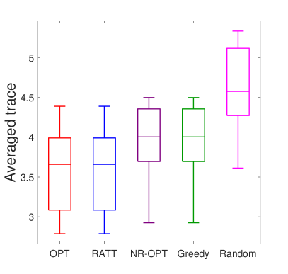
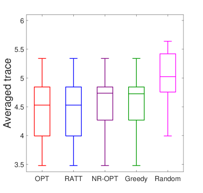
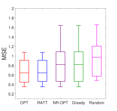
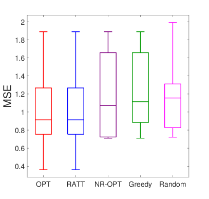
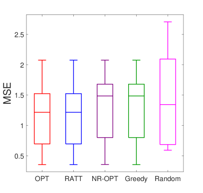
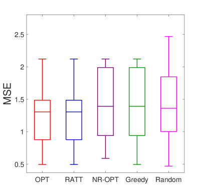
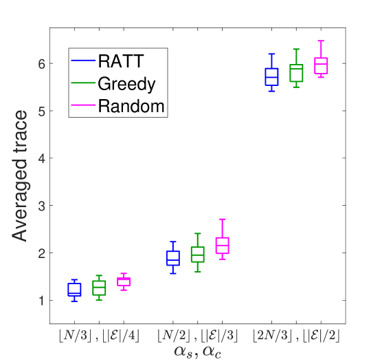
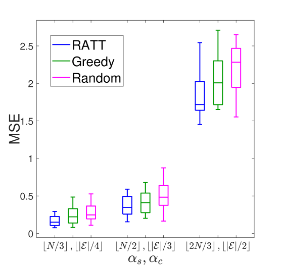
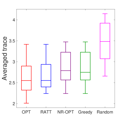
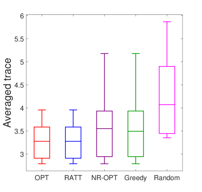
Figure 7: Comparison of the target tracking quality by OPT, RATT, NR-OPT, Greedy, and Random (averaged across 10 Monte Carlo runs): (a)-(d) depict the results of averaged trace of covariance, across four combinations of αssubscript𝛼𝑠\alpha_{s} and αcsubscript𝛼𝑐\alpha_{c} values; and (e)-(h) depict corresponding results of MSE.
Refer to caption
(a) N=10,M=15formulae-sequence𝑁10𝑀15N=10,M=15
Refer to caption
(b) N=20,M=20formulae-sequence𝑁20𝑀20N=20,M=20
Refer to caption
(c) N=30,M=25formulae-sequence𝑁30𝑀25N=30,M=25
Refer to caption
(d) N=10,M=15formulae-sequence𝑁10𝑀15N=10,M=15
Refer to caption
(e) N=20,M=20formulae-sequence𝑁20𝑀20N=20,M=20
Refer to caption
(f) N=30,M=25formulae-sequence𝑁30𝑀25N=30,M=25
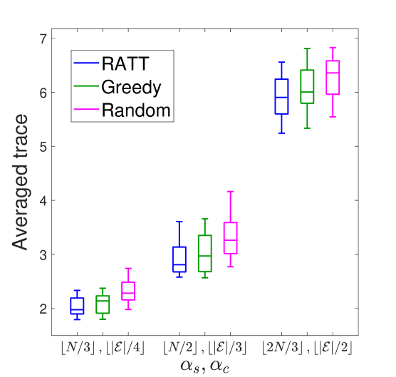
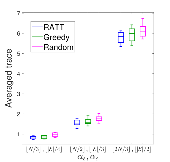
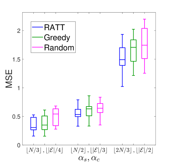
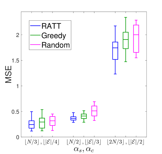
Figure 8: Comparison of the target tracking quality by RATT, Greedy, and Random (averaged across 10 Monte Carlo runs): (a)-(c) depict the results of averaged trace of covariance, across three pairs of N𝑁N and M𝑀M values, each with three combinations of αssubscript𝛼𝑠\alpha_{s} and αcsubscript𝛼𝑐\alpha_{c} values; and (e)-(h) depict corresponding results of MSE.

The results for scenario (i) are reported in Fig. 4 where the tracking quality of RATT and NR-OPT is compared without and with one sensing attack. Specifically, without the sensing attack (Fig. 4-(a) & (b)), NR-OPT attains a better tracking quality than RATT, as observed from the covariances (depicted by ellipses, capturing the uncertainty in position estimate) and the gap between the estimated mean positions (depicted by squares) and true positions (depicted by pentagrams) of the targets. This is naturally true, since NR-OPT is an optimal algorithm for non-robust target tracking. However, when there exists a sensing attack, NR-OPT loses its good tracking quality of all targets. For example, as shown in Fig. 4-(c), the tracking quality of the blue target drops sharply, as the covariance and position estimation gap increases dramatically when the sensing of the blue robot is attacked. While, as observed from Fig. 4-(d)), RATT shows its superiority against the sensing attack, since it retains a relatively good tracking quality for the two targets, with a slight increase in the estimation gap and a moderate increase in the covariance.

The results for scenarios (ii) and (iii) are reported in Fig. 5 and Fig. 6 where the tracking quality of the two algorithms is compared without and with one communication attack and without and with one sensing and two communication attacks, respectively. Fig. 5 and Fig. 6 exhibit similar results as in Fig. 4: NR-OPT performs better without the attack, but loses sharply its tracking quality for some target when the attack happens; while RATT maintains a good tracking quality for all targets, even in the presence of the communication attack or both sensing and communication attacks.

To summarize, the qualitative results in all three scenarios demonstrate the necessity for robust target tracking and the superiority of RATT against sensing and/or communication attacks.

V-B Quantitative comparison

We present quantitative results to demonstrate RATT’s superiority and robustness against sensing and communication attacks. In particular, we perform both small-scale and large-scale comparisons across various scenarios (with varying N𝑁N, M𝑀M, αssubscript𝛼𝑠\alpha_{s}, αcsubscript𝛼𝑐\alpha_{c}). For each specific scenario, the positions of robots and targets are randomly generated in the environment with robots’ headings as zero, across 10 trials. For each trial, all algorithms are executed with the same initialization, i.e., the same states of robots and targets.

Small-scale comparison

We compare the tracking quality of RATT with that of OPT, NR-OPT, Greedy, and Random. Since OPT and NR-OPT are only viable for small-scale cases, we consider small numbers of robots and targets, e.g., N=M=4𝑁𝑀4N=M=4. The algorithms are compared across four combinations of sensing and communication attacks, i.e., (αs=1,αc=3),(αs=2,αc=3),(αs=1,αc=4),(αs=2,αc=4)formulae-sequencesubscript𝛼𝑠1subscript𝛼𝑐3formulae-sequencesubscript𝛼𝑠2subscript𝛼𝑐3formulae-sequencesubscript𝛼𝑠1subscript𝛼𝑐4formulae-sequencesubscript𝛼𝑠2subscript𝛼𝑐4(\alpha_{s}=1,\alpha_{c}=3),(\alpha_{s}=2,\alpha_{c}=3),(\alpha_{s}=1,\alpha_{c}=4),(\alpha_{s}=2,\alpha_{c}=4). We evaluate these five algorithms by executing the worst-case attacks.

The comparison results are reported in Fig. 7. It is observed that RATT (colored blue) has on average a superior tracking quality to NR-OPT (colored), Greedy (colored green), and Random (colored magenta) in terms of both averaged trace of covariance and MSE. Additionally, RATT performs close to OPT (colored red), an optimal algorithm achieved by exhaustive search.

Large-scale comparison

We compare RATT’s tracking quality with that of Greedy and Random in large-scale scenarios, e.g., N[10,20,30]𝑁102030N\in[10,20,30] and M[15,20,25]𝑀152025M\in[15,20,25]. OPT is not included in the comparison due to its long evaluation time. For example, when N=10𝑁10N=10, OPT needs to evaluate |𝒰i|10superscriptsubscript𝒰𝑖10|{\mathcal{U}}_{i}|^{10} (1210superscript121012^{10}) possible cases of robots’ control inputs; for each case, its needs to evaluate (10αs)×(10×9/2αc)binomial10subscript𝛼𝑠binomial1092subscript𝛼𝑐\binom{10}{\alpha_{s}}\times\binom{10\times 9/2}{\alpha_{c}} possible cases of αssubscript𝛼𝑠\alpha_{s} sensing and αcsubscript𝛼𝑐\alpha_{c} communication attacks to find the worst-case attack; thus, in total, it takes 1210×(10αs)×(10×9/2αc)superscript1210binomial10subscript𝛼𝑠binomial1092subscript𝛼𝑐12^{10}\times\binom{10}{\alpha_{s}}\times\binom{10\times 9/2}{\alpha_{c}} to find the optimal control inputs. Evidently, OPT becomes intractable with a large number of robots.

As computed above, finding the worst-case attack requires the exhaustive search of all possible αssubscript𝛼𝑠\alpha_{s} sensing and αcsubscript𝛼𝑐\alpha_{c} communication attacks, a problem of combinatorial complexity, and thus is NP-hard [29]. Hence, when the number of robots is large, we consider the attacker to use a bounded rational attack approach, instead of executing the worst-case attack. The bounded rational attack sequentially executes two steps to attack robots’ sensing and communication: first, it removes the sensing measurements from the top αssubscript𝛼𝑠\alpha_{s} robots (whose maximum individual tracking qualities are among the top αssubscript𝛼𝑠\alpha_{s} ones in the team); second, from the remaining Nαs𝑁subscript𝛼𝑠N-\alpha_{s} robots, it blocks the communications of the top αc,ssubscript𝛼𝑐𝑠\alpha_{c,s} robots. Evidently, the bounded rational attack takes the same running time as sorting out the top α=αs+αc,s𝛼subscript𝛼𝑠subscript𝛼𝑐𝑠\alpha=\alpha_{s}+\alpha_{c,s} robots (i.e., O(Nlog(N))𝑂𝑁𝑁O(N\log(N))) and thus can be used an evaluation algorithm in large-scale scenarios.

With the bounded rational attack, the three algorithms are evaluated across three pairs of numbers of robots and targets, i.e., (N=10,M=15),(N=20,M=20),(N=30,M=25)formulae-sequence𝑁10𝑀15formulae-sequence𝑁20𝑀20formulae-sequence𝑁30𝑀25(N=10,M=15),(N=20,M=20),(N=30,M=25), each pair with three combinations of sensing and communication attacks, i.e., (αs=N/3,αc=||/4),(αs=N/2,αc=||/3)formulae-sequencesubscript𝛼𝑠𝑁3subscript𝛼𝑐4formulae-sequencesubscript𝛼𝑠𝑁2subscript𝛼𝑐3(\alpha_{s}=\left\lfloor{N/3}\right\rfloor,\alpha_{c}=\left\lfloor{|{\mathcal{E}}|/4}\right\rfloor),(\alpha_{s}=\left\lfloor{N/2}\right\rfloor,\alpha_{c}=\left\lfloor{|{\mathcal{E}}|/3}\right\rfloor), and (αs=2N/3,αc=||/2)formulae-sequencesubscript𝛼𝑠2𝑁3subscript𝛼𝑐2(\alpha_{s}=\left\lfloor{2N/3}\right\rfloor,\alpha_{c}=\left\lfloor{|{\mathcal{E}}|/2}\right\rfloor).

The comparison results are reported in Fig. 8. We observe that RATT (colored blue) is again superior to both Greedy (colored green) and Rand (colored magenta) with regard to averaged trace of covariance and MSE. Although RATT is designed to protect against worst-case attacks, it retains its superiority against bounded rational attacks.

Overall, in the quantitative evaluations above, RATT achieves a superior and close-to-optimal performance against worst-case attacks, and remains superior even against non-worst-case attacks, i.e., bounded rational attack.

VI Conclusion

We worked towards protecting critical multi-robot target tracking from sensing and communication attacks or failures. Particularly, we introduced the first robust planning framework for multi-robot tracking against any fixed numbers of worst-case sensing and communication attacks/failures (Problem 1). We provided the first robust algorithm, RATT (Algorithm 1), for Problem 1, and proved its suboptimality guarantees using the notations of curvature for set functions. With extensive empirical evaluations, we demonstrate the need for robust target tracking and RATT’s robustness and superiority against both worst-case and non-worst-case attacks.

A future direction is to extend the proposed framework to the decentralized settings [16, 17]. With decentralized communication, robustifying the team’s connectivity becomes essential to secure against communication attacks/failures. A second avenue is to investigate the proposed framework in an online resilient fashion, e.g., the receding-horizon planning [18].

Appendix

We first prove RATT’s approximation bound (Theorem 1), and then, its running time (Theorem 2).

-A Proof of Theorem 1

We prove Theorem 1, i.e., RATT’s approximation bound by capitalizing on the results in [19] which proves the approximation bound of a robust algorithm against sensing attacks. Here, we focus on the proof of RATT’s approximation bound against sensing and communication attacks. Particularly, we first prove eq. (8) where ΦΦ\Phi is merely a non-decreasing function, and then, prove eq. (9) where ΦΦ\Phi is a non-decreasing and submodular function. We start with describing necessary notations:

Notation. We introduce notations to indicate that subsets of robots whose control inputs are computed by different approaches. Specifically, we let 𝒱bsuperscript𝒱𝑏{\mathcal{V}}^{b} and 𝒱gsuperscript𝒱𝑔{\mathcal{V}}^{g} denote the subsets of robots whose control inputs are computed using the bait selection and the greedy algorithm, respectively. For simplicity, we name 𝒱bsuperscript𝒱𝑏{\mathcal{V}}^{b} and 𝒱gsuperscript𝒱𝑔{\mathcal{V}}^{g} as bait robots and greedy robots, respectively. Notably, 𝒱=𝒱b𝒱g𝒱superscript𝒱𝑏superscript𝒱𝑔{\mathcal{V}}={\mathcal{V}}^{b}\cup{\mathcal{V}}^{g}, |𝒱b|=αsuperscript𝒱𝑏𝛼|{\mathcal{V}}^{b}|=\alpha, and |𝒱g|=Nαsuperscript𝒱𝑔𝑁𝛼|{\mathcal{V}}^{g}|=N-\alpha with α=αs+αc,s𝛼subscript𝛼𝑠subscript𝛼𝑐𝑠\alpha=\alpha_{s}+\alpha_{c,s}. For a subset of robots 𝒲𝒱𝒲𝒱{\mathcal{W}}\subseteq{\mathcal{V}}, we denote 𝐮𝒲bsuperscriptsubscript𝐮𝒲𝑏{\mathbf{u}}_{{\mathcal{W}}}^{b}777For clarify, we drop the subscript for time indices. and 𝐮𝒲gsuperscriptsubscript𝐮𝒲𝑔{\mathbf{u}}_{{\mathcal{W}}}^{g} as its control inputs selected by the bait selection and the greedy algorithm, respectively. In addition, we let 𝐮𝒲subscript𝐮𝒲{\mathbf{u}}_{{\mathcal{W}}} and 𝐮𝒲superscriptsubscript𝐮𝒲{\mathbf{u}}_{{\mathcal{W}}}^{\star} denote the control inputs selected by RATT and the optimal algorithm for 𝒲𝒲{\mathcal{W}}.

Consider that the αcsubscript𝛼𝑐\alpha_{c} communication attacks separate the robot team into K𝐾K subgroups, each denoted as 𝒱k,k{1,,K}subscript𝒱𝑘𝑘1𝐾{\mathcal{V}}_{k},k\in\{1,\cdots,K\}. Clearly, 𝒱=k=1K𝒱k𝒱superscriptsubscript𝑘1𝐾subscript𝒱𝑘{\mathcal{V}}=\bigcup_{k=1}^{K}{\mathcal{V}}_{k}. Similarly, in each subgroup 𝒱ksubscript𝒱𝑘{\mathcal{V}}_{k}, we use 𝒱kbsuperscriptsubscript𝒱𝑘𝑏{\mathcal{V}}_{k}^{b} and 𝒱kgsuperscriptsubscript𝒱𝑘𝑔{\mathcal{V}}_{k}^{g} to denote the bait robots and greedy robots, respectively. Notably, 𝒱k=𝒱kb𝒱kgsubscript𝒱𝑘superscriptsubscript𝒱𝑘𝑏superscriptsubscript𝒱𝑘𝑔{\mathcal{V}}_{k}={\mathcal{V}}_{k}^{b}\cup{\mathcal{V}}_{k}^{g}, 𝒱b=k=1K𝒱kbsuperscript𝒱𝑏superscriptsubscript𝑘1𝐾superscriptsubscript𝒱𝑘𝑏{\mathcal{V}}^{b}=\bigcup_{k=1}^{K}{\mathcal{V}}_{k}^{b}, and 𝒱g=k=1K𝒱kgsuperscript𝒱𝑔superscriptsubscript𝑘1𝐾superscriptsubscript𝒱𝑘𝑔{\mathcal{V}}^{g}=\bigcup_{k=1}^{K}{\mathcal{V}}_{k}^{g}.

Recall that the worst-case communication attacks tend to separate the robot team into more, and smaller subgroups. On this basis, RATT first utilizes CAA (Algorithm (2)) to compute the number of robots in the largest subgroup as nmaxsubscript𝑛n_{\max} and approximates αcsubscript𝛼𝑐\alpha_{c} communication attacks as αc,s=Nnmaxsubscript𝛼𝑐𝑠𝑁subscript𝑛\alpha_{c,s}=N-n_{\max} sensing attacks. Indeed, by CAA and the behavior of the worst-case communication attacks, the number of subgroups and the number of robots in each subgroup after any number of the worst-case communication attacks can be exactly determined.

Then, RATT selects baits control inputs for α=αs+αc,s𝛼subscript𝛼𝑠subscript𝛼𝑐𝑠\alpha=\alpha_{s}+\alpha_{c,s} robots and the greedy control inputs for the remaining Nα𝑁𝛼N-\alpha robots by the robust maximization. Notably, |𝒱b|=|k=1K𝒱kb|=αsuperscript𝒱𝑏superscriptsubscript𝑘1𝐾superscriptsubscript𝒱𝑘𝑏𝛼|{\mathcal{V}}^{b}|=|\bigcup_{k=1}^{K}{\mathcal{V}}_{k}^{b}|=\alpha and |𝒱g|=|k=1K𝒱kg|=Nαsuperscript𝒱𝑔superscriptsubscript𝑘1𝐾superscriptsubscript𝒱𝑘𝑔𝑁𝛼|{\mathcal{V}}^{g}|=|\bigcup_{k=1}^{K}{\mathcal{V}}_{k}^{g}|=N-\alpha. Also recall that the team’s tracking quality is the tracking quality of the subgroup that performs the best (Section (II-A)-(f)). Hence, with the worse-case sensing and communication attacks, the team’s tracking quality using RATT can be written as:

Φ(𝒱𝒜s,𝒜c)=maxk{1,,K}Φ(𝐮𝒱k𝒜k),Φ𝒱superscriptsubscript𝒜𝑠superscriptsubscript𝒜𝑐subscript𝑘1𝐾Φsubscript𝐮subscript𝒱𝑘superscriptsubscript𝒜𝑘~{}\Phi({\mathcal{V}}\setminus{\mathcal{A}}_{s}^{\star},{\mathcal{E}}\setminus{\mathcal{A}}_{c}^{\star})=\max_{k\in\{1,\cdots,K\}}\Phi({\mathbf{u}}_{{\mathcal{V}}_{k}\setminus{\mathcal{A}}_{k}^{\star}}), (10)

where 𝒜ksuperscriptsubscript𝒜𝑘{\mathcal{A}}_{k}^{\star} denotes the worse-case sensing attacks in subgroup 𝒱ksubscript𝒱𝑘{\mathcal{V}}_{k}. For clarify, we omit the dependence of tracking quality ΦΦ\Phi on the communication links in each subgroup 𝒱ksubscript𝒱𝑘{\mathcal{V}}_{k}, since the robots can communicate in the same subgroup.

Correspondingly, with the worse-case sensing and communication attacks, the optimal team’s tracking quality is:

Φ𝒱,αs,,αc=maxk{1,,K}Φ(𝐮𝒱k𝒜k).superscriptsubscriptΦ𝒱subscript𝛼𝑠subscript𝛼𝑐subscript𝑘1𝐾Φsubscriptsuperscript𝐮subscript𝒱𝑘superscriptsubscript𝒜𝑘~{}\Phi_{{\mathcal{V}},\alpha_{s},{\mathcal{E}},\alpha_{c}}^{\star}=\max_{k\in\{1,\cdots,K\}}\Phi({\mathbf{u}}^{\star}_{{\mathcal{V}}_{k}\setminus{\mathcal{A}}_{k}^{\star}}). (11)

Thus, to evaluate RATT’s approximation bound Φ(𝒱𝒜s,𝒜c)/Φ𝒱,αs,,αcΦ𝒱superscriptsubscript𝒜𝑠superscriptsubscript𝒜𝑐superscriptsubscriptΦ𝒱subscript𝛼𝑠subscript𝛼𝑐\Phi({\mathcal{V}}\setminus{\mathcal{A}}_{s}^{\star},{\mathcal{E}}\setminus{\mathcal{A}}_{c}^{\star})/\Phi_{{\mathcal{V}},\alpha_{s},{\mathcal{E}},\alpha_{c}}^{\star}, we need to find out how well it does in each subgroup, i.e., Φ(𝐮𝒱k𝒜k)/Φ(𝐮𝒱k𝒜k)Φsubscript𝐮subscript𝒱𝑘superscriptsubscript𝒜𝑘Φsubscriptsuperscript𝐮subscript𝒱𝑘superscriptsubscript𝒜𝑘\Phi({\mathbf{u}}_{{\mathcal{V}}_{k}\setminus{\mathcal{A}}_{k}^{\star}})/\Phi({\mathbf{u}}^{\star}_{{\mathcal{V}}_{k}\setminus{\mathcal{A}}_{k}^{\star}}). The challenge is, even though we know the number of robots in each subgroup after αcsubscript𝛼𝑐\alpha_{c} worst-case communication attacks, we do not know exactly the robot kinds (e.g., bait and/or greedy robots) and the number of each kind in it. Also, we do not know exactly how αssubscript𝛼𝑠\alpha_{s} worst-case sensing attacking are distributed in these subgroups. To address these issues, we first explore possible patterns of robot kinds after the communication attacks, and then, under each possible pattern, we investigate possible distributions of the sensing attacks in the subgroups. Based on these possible patterns and distributions, we first prove eq. (8) and then prove eq. (9).

-A1 Proof of eq. (8)

We first consider N>α𝑁𝛼N>\alpha. In this instance, |𝒱g|=Nα>0superscript𝒱𝑔𝑁𝛼0|{\mathcal{V}}^{g}|=N-\alpha>0, and thus, there exist some greedy robots. We then consider two patterns of robot kinds after the communication attacks in the following.

  • Pattern 1: A subgroup contains αssubscript𝛼𝑠\alpha_{s} bait robots and all Nα𝑁𝛼N-\alpha greedy robots, denoted as 𝒱1subscript𝒱1{\mathcal{V}}_{1}. Notably, 𝒱1g=𝒱gsuperscriptsubscript𝒱1𝑔superscript𝒱𝑔{\mathcal{V}}_{1}^{g}={\mathcal{V}}^{g}. Other subgroups contain the remaining αc,ssubscript𝛼𝑐𝑠\alpha_{c,s} bait robots, each denoted as 𝒱k,k{2,,K}subscript𝒱𝑘𝑘2𝐾{\mathcal{V}}_{k},k\in\{2,\cdots,K\}. Notably, k=2K𝒱k=𝒱bsuperscriptsubscript𝑘2𝐾subscript𝒱𝑘superscript𝒱𝑏\bigcup_{k=2}^{K}{\mathcal{V}}_{k}={\mathcal{V}}^{b}. Under Pattern 1, we consider three possible distributions of the αssubscript𝛼𝑠\alpha_{s} worst-case sensing attacks. An example is shown in Fig. 9.
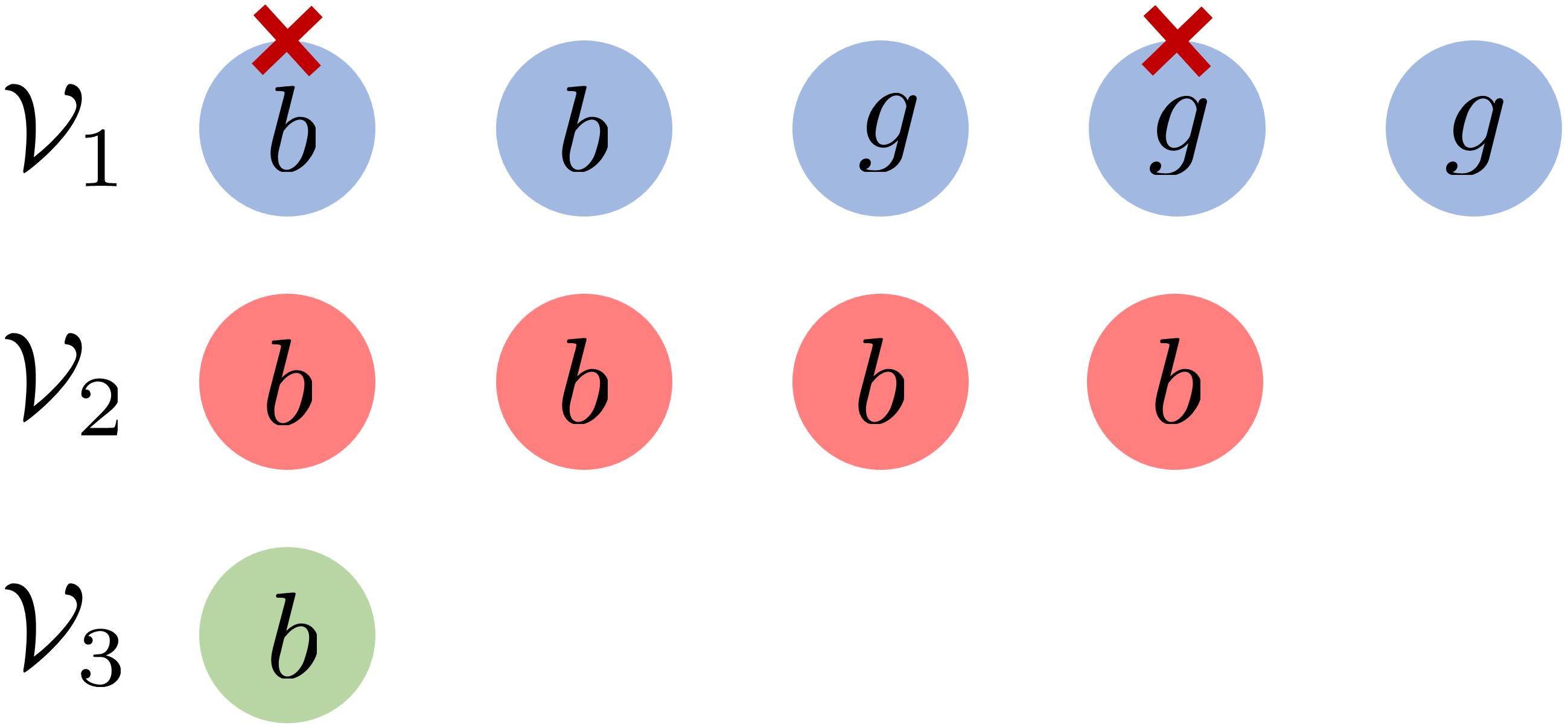
    Refer to caption
    (a) Pattern 1, Distribution 1
    Refer to caption
    (b) Pattern 1, Distribution 2
    Refer to caption
    (c) Pattern 1, Distribution 3
    Figure 9: An illustration of Pattern 1 and 3 possible distributions. Consider a team of N=10𝑁10N=10 robots encounters αs=2subscript𝛼𝑠2\alpha_{s}=2 worst-case sensing attacks (red crosses) and αc=29subscript𝛼𝑐29\alpha_{c}=29 worst-case sensing attacks. By CAA (Algorithm 2), after the 292929 worst-case communication attacks, the robot team is separated into 3 subgroups, 𝒱1subscript𝒱1{\mathcal{V}}_{1}, 𝒱2subscript𝒱2{\mathcal{V}}_{2}, 𝒱3subscript𝒱3{\mathcal{V}}_{3}. The robots in the same subgroup have the same color. The communication links in each subgroup are omitted for clarity. The number of robots in the largest clique (𝒱1subscript𝒱1{\mathcal{V}}_{1}) is nmax=5subscript𝑛5n_{\max}=5. The approximated number of sensing attacks is Nnmax=5𝑁subscript𝑛5N-n_{\max}=5. Then the total number of sensing attacks α=αs+αc,s=7𝛼subscript𝛼𝑠subscript𝛼𝑐𝑠7\alpha=\alpha_{s}+\alpha_{c,s}=7. By RATT (Algorithm 1), there are α=7𝛼7\alpha=7 bait robots (represented by “b𝑏b”) and Nα=3𝑁𝛼3N-\alpha=3 greedy robots (represented by “g𝑔g”). (a), The αs=2subscript𝛼𝑠2\alpha_{s}=2 sensing attacks are in 𝒱1subscript𝒱1{\mathcal{V}}_{1}. (b), The αs=2subscript𝛼𝑠2\alpha_{s}=2 sensing attacks are in 𝒱2subscript𝒱2{\mathcal{V}}_{2}. (c), One sensing attack is in 𝒱1subscript𝒱1{\mathcal{V}}_{1} and the other sensing attack is in 𝒱2subscript𝒱2{\mathcal{V}}_{2}.

    – Distribution 1: The αssubscript𝛼𝑠\alpha_{s} sensing attacks are in subgroup 𝒱1subscript𝒱1{\mathcal{V}}_{1} (see Fig. 9-(a)). With Distribution 1, we evaluate RATT’s approximation bound in each subgroup 𝒱ksubscript𝒱𝑘{\mathcal{V}}_{k} as follows.

    i): In subgroup 𝒱1subscript𝒱1{\mathcal{V}}_{1}, one has 𝒱1=𝒱1b𝒱1gsubscript𝒱1superscriptsubscript𝒱1𝑏superscriptsubscript𝒱1𝑔{\mathcal{V}}_{1}={\mathcal{V}}_{1}^{b}\cup{\mathcal{V}}_{1}^{g}. Notably, |𝒱1b|=αssuperscriptsubscript𝒱1𝑏subscript𝛼𝑠|{\mathcal{V}}_{1}^{b}|=\alpha_{s}, |𝒱1g|=Nαsuperscriptsubscript𝒱1𝑔𝑁𝛼|{\mathcal{V}}_{1}^{g}|=N-\alpha, and |𝒜1|=αssuperscriptsubscript𝒜1subscript𝛼𝑠|{\mathcal{A}}_{1}^{\star}|=\alpha_{s}. We evaluate RATT’s approximation bound, Φ(𝐮𝒱1𝒜1)/Φ(𝐮𝒱1𝒜1)Φsubscript𝐮subscript𝒱1superscriptsubscript𝒜1Φsubscriptsuperscript𝐮subscript𝒱1superscriptsubscript𝒜1\Phi({\mathbf{u}}_{{\mathcal{V}}_{1}\setminus{\mathcal{A}}_{1}^{\star}})/\Phi({\mathbf{u}}^{\star}_{{\mathcal{V}}_{1}\setminus{\mathcal{A}}_{1}^{\star}}), in 𝒱1subscript𝒱1{\mathcal{V}}_{1} by following [19, Proof of ineq. (8)]. Particularly,

    Φ(𝐮𝒱1𝒜1)=Φ(𝐮(𝒱1b𝒜1)(𝒱1g𝒜1)),Φsubscript𝐮subscript𝒱1superscriptsubscript𝒜1Φsubscript𝐮superscriptsubscript𝒱1𝑏superscriptsubscript𝒜1superscriptsubscript𝒱1𝑔superscriptsubscript𝒜1\displaystyle\Phi({\mathbf{u}}_{{\mathcal{V}}_{1}\setminus{\mathcal{A}}_{1}^{\star}})=\Phi({\mathbf{u}}_{({\mathcal{V}}_{1}^{b}\setminus{\mathcal{A}}_{1}^{\star})\cup({\mathcal{V}}_{1}^{g}\setminus{\mathcal{A}}_{1}^{\star})}),~{} (12)
    (1cΦ)i(𝒱1b𝒜1)(𝒱1g𝒜1)Φ(𝐮i),absent1subscript𝑐Φsubscript𝑖superscriptsubscript𝒱1𝑏superscriptsubscript𝒜1superscriptsubscript𝒱1𝑔superscriptsubscript𝒜1Φsubscript𝐮𝑖\displaystyle\geq(1-c_{\Phi})\sum_{i\in({\mathcal{V}}_{1}^{b}\setminus{\mathcal{A}}_{1}^{\star})\cup({\mathcal{V}}_{1}^{g}\setminus{\mathcal{A}}_{1}^{\star})}\Phi({\mathbf{u}}_{i}),~{} (13)
    =(1cΦ)[i𝒱1b𝒜1Φ(𝐮ib)+i𝒱1g𝒜1Φ(𝐮ig)],absent1subscript𝑐Φdelimited-[]subscript𝑖superscriptsubscript𝒱1𝑏superscriptsubscript𝒜1Φsubscriptsuperscript𝐮𝑏𝑖subscript𝑖superscriptsubscript𝒱1𝑔superscriptsubscript𝒜1Φsubscriptsuperscript𝐮𝑔𝑖\displaystyle=(1-c_{\Phi})[\sum_{i\in{\mathcal{V}}_{1}^{b}\setminus{\mathcal{A}}_{1}^{\star}}\Phi({\mathbf{u}}^{b}_{i})+\sum_{i\in{\mathcal{V}}_{1}^{g}\setminus{\mathcal{A}}_{1}^{\star}}\Phi({\mathbf{u}}^{g}_{i})],~{} (14)
    (1cΦ)[i𝒱1g(𝒱1g𝒜1)Φ(𝐮ig)+i𝒱1g𝒜1Φ(𝐮ig)],absent1subscript𝑐Φdelimited-[]subscript𝑖superscriptsubscript𝒱1𝑔superscriptsubscript𝒱1𝑔superscriptsubscript𝒜1Φsubscriptsuperscript𝐮𝑔𝑖subscript𝑖superscriptsubscript𝒱1𝑔superscriptsubscript𝒜1Φsubscriptsuperscript𝐮𝑔𝑖\displaystyle\geq(1-c_{\Phi})[\sum_{i\in{\mathcal{V}}_{1}^{g}\setminus({\mathcal{V}}_{1}^{g}\setminus{\mathcal{A}}_{1}^{\star})}\Phi({\mathbf{u}}^{g}_{i})+\sum_{i\in{\mathcal{V}}_{1}^{g}\setminus{\mathcal{A}}_{1}^{\star}}\Phi({\mathbf{u}}^{g}_{i})],~{} (15)
    =(1cΦ)i𝒱1gΦ(𝐮ig),absent1subscript𝑐Φsubscript𝑖superscriptsubscript𝒱1𝑔Φsubscriptsuperscript𝐮𝑔𝑖\displaystyle=(1-c_{\Phi})\sum_{i\in{\mathcal{V}}_{1}^{g}}\Phi({\mathbf{u}}^{g}_{i}),~{} (16)
    (1cΦ)2Φ(𝐮𝒱1gg),absentsuperscript1subscript𝑐Φ2Φsubscriptsuperscript𝐮𝑔superscriptsubscript𝒱1𝑔\displaystyle\geq(1-c_{\Phi})^{2}\Phi({\mathbf{u}}^{g}_{{\mathcal{V}}_{1}^{g}}),~{} (17)
    (1cΦ)3Φ(𝐮𝒱1g),absentsuperscript1subscript𝑐Φ3Φsubscriptsuperscript𝐮superscriptsubscript𝒱1𝑔\displaystyle\geq(1-c_{\Phi})^{3}\Phi({\mathbf{u}}^{\star}_{{\mathcal{V}}_{1}^{g}}),~{} (18)
    (1cΦ)3Φ(𝐮𝒱1𝒜1).absentsuperscript1subscript𝑐Φ3Φsubscriptsuperscript𝐮subscript𝒱1superscriptsubscript𝒜1\displaystyle\geq(1-c_{\Phi})^{3}\Phi({\mathbf{u}}^{\star}_{{\mathcal{V}}_{1}\setminus{\mathcal{A}}_{1}^{\star}}).~{} (19)

    Eqs. (12) - (19) hold for the following reasons. Eq. (12) holds since 𝒱1=𝒱1b+𝒱1gsubscript𝒱1superscriptsubscript𝒱1𝑏superscriptsubscript𝒱1𝑔{\mathcal{V}}_{1}={\mathcal{V}}_{1}^{b}+{\mathcal{V}}_{1}^{g}. Ineq. (13) follows from eq. (12) due to [19, Lemma 4], which is derived based on the definition of the total curvature (eq. (7)). Eq. (14) follows from ineq. (13) due to (𝒱1b𝒜1)(𝒱1b𝒜1)=superscriptsubscript𝒱1𝑏superscriptsubscript𝒜1superscriptsubscript𝒱1𝑏superscriptsubscript𝒜1({\mathcal{V}}_{1}^{b}\setminus{\mathcal{A}}_{1}^{\star})\cap({\mathcal{V}}_{1}^{b}\setminus{\mathcal{A}}_{1}^{\star})=\emptyset. Ineq. (15) holds because: first, since 𝒱1bsuperscriptsubscript𝒱1𝑏{\mathcal{V}}_{1}^{b} are bait robots and 𝒱1gsuperscriptsubscript𝒱1𝑔{\mathcal{V}}_{1}^{g} are greedy robots, Φ(𝐮ib)Φ(𝐮ig)Φsubscriptsuperscript𝐮𝑏𝑖Φsubscriptsuperscript𝐮𝑔superscript𝑖\Phi({\mathbf{u}}^{b}_{i})\geq\Phi({\mathbf{u}}^{g}_{i^{\prime}}) for any i𝒱1b𝒜1𝑖superscriptsubscript𝒱1𝑏superscriptsubscript𝒜1i\in{\mathcal{V}}_{1}^{b}\setminus{\mathcal{A}}_{1}^{\star} and i𝒱1g𝒜1superscript𝑖superscriptsubscript𝒱1𝑔superscriptsubscript𝒜1i^{\prime}\in{\mathcal{V}}_{1}^{g}\setminus{\mathcal{A}}_{1}^{\star}; second, since 𝒱1b𝒜1superscriptsubscript𝒱1𝑏superscriptsubscript𝒜1{\mathcal{V}}_{1}^{b}\setminus{\mathcal{A}}_{1}^{\star} and 𝒱1g𝒜1superscriptsubscript𝒱1𝑔superscriptsubscript𝒜1{\mathcal{V}}_{1}^{g}\setminus{\mathcal{A}}_{1}^{\star} denote respectively the set of non-attacked robots in 𝒱1bsuperscriptsubscript𝒱1𝑏{\mathcal{V}}_{1}^{b} and the set of non-attacked robots in 𝒱1gsuperscriptsubscript𝒱1𝑔{\mathcal{V}}_{1}^{g} after the worst-case sensing attacks 𝒜1superscriptsubscript𝒜1{\mathcal{A}}_{1}^{\star}, one has |𝒱1b𝒜1|+|𝒱1g𝒜1|=αssuperscriptsubscript𝒱1𝑏superscriptsubscript𝒜1superscriptsubscript𝒱1𝑔superscriptsubscript𝒜1subscript𝛼𝑠|{\mathcal{V}}_{1}^{b}\cap{\mathcal{A}}_{1}^{\star}|+|{\mathcal{V}}_{1}^{g}\cap{\mathcal{A}}_{1}^{\star}|=\alpha_{s}, and thus |𝒱1b𝒜1|=αs|𝒱1b𝒜1|=|𝒱1g𝒜1|=|𝒱1g(𝒱1g𝒜1)|superscriptsubscript𝒱1𝑏superscriptsubscript𝒜1subscript𝛼𝑠superscriptsubscript𝒱1𝑏superscriptsubscript𝒜1superscriptsubscript𝒱1𝑔superscriptsubscript𝒜1superscriptsubscript𝒱1𝑔superscriptsubscript𝒱1𝑔superscriptsubscript𝒜1|{\mathcal{V}}_{1}^{b}\setminus{\mathcal{A}}_{1}^{\star}|=\alpha_{s}-|{\mathcal{V}}_{1}^{b}\cap{\mathcal{A}}_{1}^{\star}|=|{\mathcal{V}}_{1}^{g}\cap{\mathcal{A}}_{1}^{\star}|=|{\mathcal{V}}_{1}^{g}\setminus({\mathcal{V}}_{1}^{g}\setminus{\mathcal{A}}_{1}^{\star})|. Eq. (16) follows naturally from ineq. (15). Ineq. (17) follows from eq. (16) due to [19, Corollary 1], which is derived by using the property of the total curvature (eq. (7)). Ineq. (18) follows from ineq. (17) due to [21, Theorem 8.1], which implies that the greedy algorithm, introduced in [22, Section 2], achieves 1cΦ1subscript𝑐Φ1-c_{\Phi} approximation bound for optimizing non-decreasing functions. Ineq. (19) follows from ineq. (18) due to [19, Lemma 9].

    ii): In each of the other subgroups 𝒱k,k{2,,K}subscript𝒱𝑘𝑘2𝐾{\mathcal{V}}_{k},k\in\{2,\cdots,K\}, there exist no sensing attacks (𝒜k=superscriptsubscript𝒜𝑘{\mathcal{A}}_{k}^{\star}=\emptyset) and the robots’ control inputs are bait control inputs. Hence,

    Φ(𝐮𝒱k𝒜k)Φsubscript𝐮subscript𝒱𝑘superscriptsubscript𝒜𝑘\displaystyle\Phi({\mathbf{u}}_{{\mathcal{V}}_{k}\setminus{\mathcal{A}}_{k}^{\star}}) =Φ(𝐮𝒱kb)absentΦsubscriptsuperscript𝐮𝑏subscript𝒱𝑘\displaystyle=\Phi({\mathbf{u}}^{b}_{{\mathcal{V}}_{k}})~{} (20)
    (1cΦ)i𝒱kΦ(𝐮ib),absent1subscript𝑐Φsubscript𝑖subscript𝒱𝑘Φsubscriptsuperscript𝐮𝑏𝑖\displaystyle\geq(1-c_{\Phi})\sum_{i\in{\mathcal{V}}_{k}}\Phi({\mathbf{u}}^{b}_{i}),~{} (21)
    =(1cΦ)i𝒱kΦ(𝐮i),absent1subscript𝑐Φsubscript𝑖subscript𝒱𝑘Φsuperscriptsubscript𝐮𝑖\displaystyle=(1-c_{\Phi})\sum_{i\in{\mathcal{V}}_{k}}\Phi({\mathbf{u}}_{i}^{\star}),~{} (22)
    (1cΦ)2Φ(𝐮𝒱k).absentsuperscript1subscript𝑐Φ2Φsubscriptsuperscript𝐮subscript𝒱𝑘\displaystyle\geq(1-c_{\Phi})^{2}\Phi({\mathbf{u}}^{\star}_{{\mathcal{V}}_{k}}).~{} (23)
    =(1cΦ)2Φ(𝐮𝒱k𝒜k).absentsuperscript1subscript𝑐Φ2Φsubscriptsuperscript𝐮subscript𝒱𝑘superscriptsubscript𝒜𝑘\displaystyle=(1-c_{\Phi})^{2}\Phi({\mathbf{u}}^{\star}_{{\mathcal{V}}_{k}\setminus{\mathcal{A}}_{k}^{\star}}).~{} (24)

    Eqs. (20) - (24) hold for the following reasons. Eq. (20) holds since 𝒜k=superscriptsubscript𝒜𝑘{\mathcal{A}}_{k}^{\star}=\emptyset and 𝒱k=𝒱kbsubscript𝒱𝑘superscriptsubscript𝒱𝑘𝑏{\mathcal{V}}_{k}={\mathcal{V}}_{k}^{b}. Ineq. (21) follows from eq. (20) due to [19, Lemma 4]. Eq. (22) follows from ineq. (21) since each bait control input 𝐮ibsuperscriptsubscript𝐮𝑖𝑏{\mathbf{u}}_{i}^{b} gives the maximum individual tracking quality. Ineq. (23) follows from eq. (22) due to [19, Corollary 1] and 𝒜k=superscriptsubscript𝒜𝑘{\mathcal{A}}_{k}^{\star}=\emptyset. Ineq. (24) follows from ineq. (23) due to 𝒜k=superscriptsubscript𝒜𝑘{\mathcal{A}}_{k}^{\star}=\emptyset.

    To sum up, in Pattern 1, Distribution 1, by eqs. (12) - (19) and eqs. (20)-(24), one has

    maxk{1,,K}Φ(𝐮𝒱k𝒜k)subscript𝑘1𝐾Φsubscript𝐮subscript𝒱𝑘superscriptsubscript𝒜𝑘\displaystyle\max_{k\in\{1,\cdots,K\}}\Phi({\mathbf{u}}_{{\mathcal{V}}_{k}\setminus{\mathcal{A}}_{k}^{\star}})
    min[(1cΦ)2,(1cΦ)3]maxk{1,,K}Φ(𝐮𝒱k𝒜k).absentsuperscript1subscript𝑐Φ2superscript1subscript𝑐Φ3subscript𝑘1𝐾Φsubscriptsuperscript𝐮subscript𝒱𝑘superscriptsubscript𝒜𝑘\displaystyle\geq\min[(1-c_{\Phi})^{2},(1-c_{\Phi})^{3}]\max_{k\in\{1,\cdots,K\}}\Phi({\mathbf{u}}^{\star}_{{\mathcal{V}}_{k}\setminus{\mathcal{A}}_{k}^{\star}}).

    Therefore, along with eqs. (10) and (11), one has

    Φ(𝒱,𝒜c)(1cΦ)3Φ𝒱,αs,,αc.Φ𝒱superscriptsubscript𝒜𝑐superscript1subscript𝑐Φ3superscriptsubscriptΦ𝒱subscript𝛼𝑠subscript𝛼𝑐\Phi({\mathcal{V}}\setminus\emptyset,{\mathcal{E}}\setminus{\mathcal{A}}_{c}^{\star})\geq(1-c_{\Phi})^{3}\Phi_{{\mathcal{V}},\alpha_{s},{\mathcal{E}},\alpha_{c}}^{\star}. (25)

    – Distribution 2: The αssubscript𝛼𝑠\alpha_{s} sensing attacks are in subgroups {𝒱k}k=2Ksuperscriptsubscriptsubscript𝒱𝑘𝑘2𝐾\{{\mathcal{V}}_{k}\}_{k=2}^{K} (see Fig. 9-(b)). With Distribution 2, we evaluate RATT’s approximation bound in each subgroup 𝒱ksubscript𝒱𝑘{\mathcal{V}}_{k} as follows.

    i): In subgroup 𝒱1subscript𝒱1{\mathcal{V}}_{1}, one has 𝒱1=𝒱1b𝒱1gsubscript𝒱1superscriptsubscript𝒱1𝑏superscriptsubscript𝒱1𝑔{\mathcal{V}}_{1}={\mathcal{V}}_{1}^{b}\cup{\mathcal{V}}_{1}^{g}. Notably, |𝒱1b|=αssuperscriptsubscript𝒱1𝑏subscript𝛼𝑠|{\mathcal{V}}_{1}^{b}|=\alpha_{s}, |𝒱1g|=Nαsuperscriptsubscript𝒱1𝑔𝑁𝛼|{\mathcal{V}}_{1}^{g}|=N-\alpha, and 𝒜1=superscriptsubscript𝒜1{\mathcal{A}}_{1}^{\star}=\emptyset. Hence,

    Φ(𝐮𝒱1𝒜1)=Φ(𝐮𝒱1b𝒱1g),Φsubscript𝐮subscript𝒱1superscriptsubscript𝒜1Φsubscript𝐮superscriptsubscript𝒱1𝑏superscriptsubscript𝒱1𝑔\displaystyle\Phi({\mathbf{u}}_{{\mathcal{V}}_{1}\setminus{\mathcal{A}}_{1}^{\star}})=\Phi({\mathbf{u}}_{{\mathcal{V}}_{1}^{b}\cup{\mathcal{V}}_{1}^{g}}),~{} (26)
    (1cΦ)i𝒱1b𝒱1gΦ(𝐮i),absent1subscript𝑐Φsubscript𝑖superscriptsubscript𝒱1𝑏superscriptsubscript𝒱1𝑔Φsubscript𝐮𝑖\displaystyle\geq(1-c_{\Phi})\sum_{i\in{\mathcal{V}}_{1}^{b}\cup{\mathcal{V}}_{1}^{g}}\Phi({\mathbf{u}}_{i}),~{} (27)
    =(1cΦ)[i𝒱1bΦ(𝐮ib)+i𝒱1gΦ(𝐮ig)],absent1subscript𝑐Φdelimited-[]subscript𝑖superscriptsubscript𝒱1𝑏Φsubscriptsuperscript𝐮𝑏𝑖subscript𝑖superscriptsubscript𝒱1𝑔Φsubscriptsuperscript𝐮𝑔𝑖\displaystyle=(1-c_{\Phi})[\sum_{i\in{\mathcal{V}}_{1}^{b}}\Phi({\mathbf{u}}^{b}_{i})+\sum_{i\in{\mathcal{V}}_{1}^{g}}\Phi({\mathbf{u}}^{g}_{i})],~{} (28)
    =(1cΦ)[i𝒱1bΦ(𝐮i)+i𝒱1gΦ(𝐮ig)],absent1subscript𝑐Φdelimited-[]subscript𝑖superscriptsubscript𝒱1𝑏Φsubscriptsuperscript𝐮𝑖subscript𝑖superscriptsubscript𝒱1𝑔Φsubscriptsuperscript𝐮𝑔𝑖\displaystyle=(1-c_{\Phi})[\sum_{i\in{\mathcal{V}}_{1}^{b}}\Phi({\mathbf{u}}^{\star}_{i})+\sum_{i\in{\mathcal{V}}_{1}^{g}}\Phi({\mathbf{u}}^{g}_{i})],~{} (29)
    (1cΦ)2[Φ(𝐮𝒱1b)+Φ(𝐮𝒱1gg)],absentsuperscript1subscript𝑐Φ2delimited-[]Φsubscriptsuperscript𝐮superscriptsubscript𝒱1𝑏Φsubscriptsuperscript𝐮𝑔superscriptsubscript𝒱1𝑔\displaystyle\geq(1-c_{\Phi})^{2}[\Phi({\mathbf{u}}^{\star}_{{\mathcal{V}}_{1}^{b}})+\Phi({\mathbf{u}}^{g}_{{\mathcal{V}}_{1}^{g}})],~{} (30)
    (1cΦ)2Φ(𝐮𝒱1b)+(1cΦ)3Φ(𝐮𝒱1g),absentsuperscript1subscript𝑐Φ2Φsubscriptsuperscript𝐮superscriptsubscript𝒱1𝑏superscript1subscript𝑐Φ3Φsubscriptsuperscript𝐮superscriptsubscript𝒱1𝑔\displaystyle\geq(1-c_{\Phi})^{2}\Phi({\mathbf{u}}^{\star}_{{\mathcal{V}}_{1}^{b}})+(1-c_{\Phi})^{3}\Phi({\mathbf{u}}^{\star}_{{\mathcal{V}}_{1}^{g}}),~{} (31)
    (1cΦ)3[Φ(𝐮𝒱1b)+Φ(𝐮𝒱1g)],absentsuperscript1subscript𝑐Φ3delimited-[]Φsubscriptsuperscript𝐮superscriptsubscript𝒱1𝑏Φsubscriptsuperscript𝐮superscriptsubscript𝒱1𝑔\displaystyle\geq(1-c_{\Phi})^{3}[\Phi({\mathbf{u}}^{\star}_{{\mathcal{V}}_{1}^{b}})+\Phi({\mathbf{u}}^{\star}_{{\mathcal{V}}_{1}^{g}})],~{} (32)
    (1cΦ)3Φ(𝐮𝒱1),absentsuperscript1subscript𝑐Φ3Φsubscriptsuperscript𝐮subscript𝒱1\displaystyle\geq(1-c_{\Phi})^{3}\Phi({\mathbf{u}}^{\star}_{{\mathcal{V}}_{1}}),~{} (33)
    =(1cΦ)3Φ(𝐮𝒱1𝒜1).absentsuperscript1subscript𝑐Φ3Φsubscriptsuperscript𝐮subscript𝒱1superscriptsubscript𝒜1\displaystyle=(1-c_{\Phi})^{3}\Phi({\mathbf{u}}^{\star}_{{\mathcal{V}}_{1}\setminus{\mathcal{A}}_{1}^{\star}}).~{} (34)

    Eqs. (26) - (34) hold for the following reasons. Eq. (26) holds since 𝒜1=superscriptsubscript𝒜1{\mathcal{A}}_{1}^{\star}=\emptyset and 𝒱1=𝒱1b𝒱1gsubscript𝒱1superscriptsubscript𝒱1𝑏superscriptsubscript𝒱1𝑔{\mathcal{V}}_{1}={\mathcal{V}}_{1}^{b}\cup{\mathcal{V}}_{1}^{g}. Ineq. (27) follows from eq. (26) due to [19, Lemma 4]. Eq. (28) naturally follows from ineq. (27) due to 𝒱1b𝒱1g=superscriptsubscript𝒱1𝑏superscriptsubscript𝒱1𝑔{\mathcal{V}}_{1}^{b}\cap{\mathcal{V}}_{1}^{g}=\emptyset. Eq. (29) follows from eq. (28) since each bait control input 𝐮ibsuperscriptsubscript𝐮𝑖𝑏{\mathbf{u}}_{i}^{b} gives the maximum individual tracking quality. Ineq. (30) follows from eq. (29) due to [19, Corollary 1]. Ineq. (31) follows from ineq. (30) due to [21, Theorem 8.1], which implies that the greedy algorithm [22, Section 2] achieves 1cΦ1subscript𝑐Φ1-c_{\Phi} approximation bound for optimizing non-decreasing functions, and thus Φ(𝐮𝒱1gg)(1cΦ)Φ(𝐮𝒱1g)Φsubscriptsuperscript𝐮𝑔superscriptsubscript𝒱1𝑔1subscript𝑐ΦΦsubscriptsuperscript𝐮superscriptsubscript𝒱1𝑔\Phi({\mathbf{u}}^{g}_{{\mathcal{V}}_{1}^{g}})\geq(1-c_{\Phi})\Phi({\mathbf{u}}^{\star}_{{\mathcal{V}}_{1}^{g}}). Ineq. (32) follows from ineq. (31) due to 1cΦ[0,1]1subscript𝑐Φ011-c_{\Phi}\in[0,1]. Ineq. (33) follows from ineq. (32) due to 𝒱1b,𝒱1g𝒱1superscriptsubscript𝒱1𝑏superscriptsubscript𝒱1𝑔subscript𝒱1{\mathcal{V}}_{1}^{b},{\mathcal{V}}_{1}^{g}\subseteq{\mathcal{V}}_{1}, 𝒱1b𝒱1g=superscriptsubscript𝒱1𝑏superscriptsubscript𝒱1𝑔{\mathcal{V}}_{1}^{b}\cap{\mathcal{V}}_{1}^{g}=\emptyset, and thus Φ(𝐮𝒱1b)+Φ(𝐮𝒱1g)Φ(𝐮𝒱1)Φsubscriptsuperscript𝐮superscriptsubscript𝒱1𝑏Φsubscriptsuperscript𝐮superscriptsubscript𝒱1𝑔Φsubscriptsuperscript𝐮subscript𝒱1\Phi({\mathbf{u}}^{\star}_{{\mathcal{V}}_{1}^{b}})+\Phi({\mathbf{u}}^{\star}_{{\mathcal{V}}_{1}^{g}})\geq\Phi({\mathbf{u}}^{\star}_{{\mathcal{V}}_{1}}). Eq. (34) follows from ineq. (33) due to 𝒜1=superscriptsubscript𝒜1{\mathcal{A}}_{1}^{\star}=\emptyset.

    ii): In the other subgroups {𝒱k}k=2Ksuperscriptsubscriptsubscript𝒱𝑘𝑘2𝐾\{{\mathcal{V}}_{k}\}_{k=2}^{K}, even though there exist αssubscript𝛼𝑠\alpha_{s} sensing attacks, the control inputs of the non-attacked robots are still bait control inputs. Hence, in each subgroup 𝒱ksubscript𝒱𝑘{\mathcal{V}}_{k}, one has,

    Φ(𝐮𝒱k𝒜k)Φsubscript𝐮subscript𝒱𝑘superscriptsubscript𝒜𝑘\displaystyle\Phi({\mathbf{u}}_{{\mathcal{V}}_{k}\setminus{\mathcal{A}}_{k}^{\star}}) =Φ(𝐮𝒱k𝒜kb)absentΦsubscriptsuperscript𝐮𝑏subscript𝒱𝑘superscriptsubscript𝒜𝑘\displaystyle=\Phi({\mathbf{u}}^{b}_{{\mathcal{V}}_{k}\setminus{\mathcal{A}}_{k}^{\star}})~{} (35)
    (1cΦ)i𝒱k𝒜kΦ(𝐮ib),absent1subscript𝑐Φsubscript𝑖subscript𝒱𝑘superscriptsubscript𝒜𝑘Φsubscriptsuperscript𝐮𝑏𝑖\displaystyle\geq(1-c_{\Phi})\sum_{i\in{\mathcal{V}}_{k}\setminus{\mathcal{A}}_{k}^{\star}}\Phi({\mathbf{u}}^{b}_{i}),~{} (36)
    =(1cΦ)i𝒱k𝒜kΦ(𝐮i),absent1subscript𝑐Φsubscript𝑖subscript𝒱𝑘superscriptsubscript𝒜𝑘Φsuperscriptsubscript𝐮𝑖\displaystyle=(1-c_{\Phi})\sum_{i\in{\mathcal{V}}_{k}\setminus{\mathcal{A}}_{k}^{\star}}\Phi({\mathbf{u}}_{i}^{\star}),~{} (37)
    (1cΦ)2Φ(𝐮𝒱k𝒜k).absentsuperscript1subscript𝑐Φ2Φsubscriptsuperscript𝐮subscript𝒱𝑘superscriptsubscript𝒜𝑘\displaystyle\geq(1-c_{\Phi})^{2}\Phi({\mathbf{u}}^{\star}_{{\mathcal{V}}_{k}\setminus{\mathcal{A}}_{k}^{\star}}).~{} (38)

    Eqs. (35) - (38) hold for the following reasons. Eq. (35) holds since 𝒱k=𝒱kbsubscript𝒱𝑘superscriptsubscript𝒱𝑘𝑏{\mathcal{V}}_{k}={\mathcal{V}}_{k}^{b}. Ineq. (36) follows from eq. (35) due to [19, Lemma 4]. Eq. (37) follows from ineq. (36) since each bait control input 𝐮ibsuperscriptsubscript𝐮𝑖𝑏{\mathbf{u}}_{i}^{b} gives the maximum individual tracking quality. Ineq. (38) follows from eq. (37) due to [19, Corollary 1].

    To sum up, in Pattern 1, Distribution 2, by eqs. (26) - (34) and eqs. (35)-(38), one has

    maxk{1,,K}Φ(𝐮𝒱k𝒜k)subscript𝑘1𝐾Φsubscript𝐮subscript𝒱𝑘superscriptsubscript𝒜𝑘\displaystyle\max_{k\in\{1,\cdots,K\}}\Phi({\mathbf{u}}_{{\mathcal{V}}_{k}\setminus{\mathcal{A}}_{k}^{\star}})
    min[(1cΦ)2,(1cΦ)3]maxk{1,,K}Φ(𝐮𝒱k𝒜k).absentsuperscript1subscript𝑐Φ2superscript1subscript𝑐Φ3subscript𝑘1𝐾Φsubscriptsuperscript𝐮subscript𝒱𝑘superscriptsubscript𝒜𝑘\displaystyle\geq\min[(1-c_{\Phi})^{2},(1-c_{\Phi})^{3}]\max_{k\in\{1,\cdots,K\}}\Phi({\mathbf{u}}^{\star}_{{\mathcal{V}}_{k}\setminus{\mathcal{A}}_{k}^{\star}}).

    Therefore, along with eqs. (10) and (11), one has

    Φ(𝒱,𝒜c)(1cΦ)3Φ𝒱,αs,,αc.Φ𝒱superscriptsubscript𝒜𝑐superscript1subscript𝑐Φ3superscriptsubscriptΦ𝒱subscript𝛼𝑠subscript𝛼𝑐\Phi({\mathcal{V}}\setminus\emptyset,{\mathcal{E}}\setminus{\mathcal{A}}_{c}^{\star})\geq(1-c_{\Phi})^{3}\Phi_{{\mathcal{V}},\alpha_{s},{\mathcal{E}},\alpha_{c}}^{\star}. (39)

    – Distribution 3: Part of the αssubscript𝛼𝑠\alpha_{s} sensing attacks (i.e., αs1superscriptsubscript𝛼𝑠1\alpha_{s}^{1}, αs1<αssuperscriptsubscript𝛼𝑠1subscript𝛼𝑠\alpha_{s}^{1}<\alpha_{s}) is in subgroup 𝒱1subscript𝒱1{\mathcal{V}}_{1} and the remaining part (i.e., αsαs1subscript𝛼𝑠superscriptsubscript𝛼𝑠1\alpha_{s}-\alpha_{s}^{1}) is in subgroups {𝒱k}k=2Ksuperscriptsubscriptsubscript𝒱𝑘𝑘2𝐾\{{\mathcal{V}}_{k}\}_{k=2}^{K} (see Fig. 9-(c)).

    i): In subgroup 𝒱1subscript𝒱1{\mathcal{V}}_{1}, one has 𝒱1=𝒱1b𝒱1gsubscript𝒱1superscriptsubscript𝒱1𝑏superscriptsubscript𝒱1𝑔{\mathcal{V}}_{1}={\mathcal{V}}_{1}^{b}\cup{\mathcal{V}}_{1}^{g}. Notably, |𝒱1b|=αssuperscriptsubscript𝒱1𝑏subscript𝛼𝑠|{\mathcal{V}}_{1}^{b}|=\alpha_{s}, |𝒱1g|=Nαsuperscriptsubscript𝒱1𝑔𝑁𝛼|{\mathcal{V}}_{1}^{g}|=N-\alpha, and |𝒜1|=αs1superscriptsubscript𝒜1superscriptsubscript𝛼𝑠1|{\mathcal{A}}_{1}^{\star}|=\alpha_{s}^{1}. Since the number of sensing attacks αs1superscriptsubscript𝛼𝑠1\alpha_{s}^{1} in 𝒱1subscript𝒱1{\mathcal{V}}_{1} is less than αssubscript𝛼𝑠\alpha_{s}, there must exist a subset of αsαs1subscript𝛼𝑠superscriptsubscript𝛼𝑠1\alpha_{s}-\alpha_{s}^{1} robots that does not encounter sensing attacks in 𝒱1bsuperscriptsubscript𝒱1𝑏{\mathcal{V}}_{1}^{b}. We denote this subset as 𝒱1b1𝒱1bsuperscriptsubscript𝒱1𝑏1superscriptsubscript𝒱1𝑏{\mathcal{V}}_{1}^{b1}\subseteq{\mathcal{V}}_{1}^{b} with |𝒱1b1|=ααs1superscriptsubscript𝒱1𝑏1𝛼superscriptsubscript𝛼𝑠1|{\mathcal{V}}_{1}^{b1}|=\alpha-\alpha_{s}^{1}. In addition, denote the other robots in 𝒱1b1superscriptsubscript𝒱1𝑏1{\mathcal{V}}_{1}^{b1} as 𝒱1b2=𝒱1b𝒱1b1superscriptsubscript𝒱1𝑏2superscriptsubscript𝒱1𝑏superscriptsubscript𝒱1𝑏1{\mathcal{V}}_{1}^{b2}={\mathcal{V}}_{1}^{b}\setminus{\mathcal{V}}_{1}^{b1}. Notably, |𝒱1b2|=αs1superscriptsubscript𝒱1𝑏2superscriptsubscript𝛼𝑠1|{\mathcal{V}}_{1}^{b2}|=\alpha_{s}^{1}. Then, we evaluate RATT’s approximation bound, Φ(𝐮𝒱1𝒜1)/Φ(𝐮𝒱1𝒜1)Φsubscript𝐮subscript𝒱1superscriptsubscript𝒜1Φsubscriptsuperscript𝐮subscript𝒱1superscriptsubscript𝒜1\Phi({\mathbf{u}}_{{\mathcal{V}}_{1}\setminus{\mathcal{A}}_{1}^{\star}})/\Phi({\mathbf{u}}^{\star}_{{\mathcal{V}}_{1}\setminus{\mathcal{A}}_{1}^{\star}}), in 𝒱1subscript𝒱1{\mathcal{V}}_{1} as follows.

    Φ(𝐮𝒱1𝒜1)=Φ(𝐮(𝒱1b𝒜1)(𝒱1g𝒜1)),Φsubscript𝐮subscript𝒱1superscriptsubscript𝒜1Φsubscript𝐮superscriptsubscript𝒱1𝑏superscriptsubscript𝒜1superscriptsubscript𝒱1𝑔superscriptsubscript𝒜1\displaystyle\Phi({\mathbf{u}}_{{\mathcal{V}}_{1}\setminus{\mathcal{A}}_{1}^{\star}})=\Phi({\mathbf{u}}_{({\mathcal{V}}_{1}^{b}\setminus{\mathcal{A}}_{1}^{\star})\cup({\mathcal{V}}_{1}^{g}\setminus{\mathcal{A}}_{1}^{\star})}),~{} (40)
    (1cΦ)i(𝒱1b𝒜1)(𝒱1g𝒜1)Φ(𝐮i),absent1subscript𝑐Φsubscript𝑖superscriptsubscript𝒱1𝑏superscriptsubscript𝒜1superscriptsubscript𝒱1𝑔superscriptsubscript𝒜1Φsubscript𝐮𝑖\displaystyle\geq(1-c_{\Phi})\sum_{i\in({\mathcal{V}}_{1}^{b}\setminus{\mathcal{A}}_{1}^{\star})\cup({\mathcal{V}}_{1}^{g}\setminus{\mathcal{A}}_{1}^{\star})}\Phi({\mathbf{u}}_{i}),~{} (41)
    =(1cΦ)[i𝒱1b1Φ(𝐮ib)+\displaystyle=(1-c_{\Phi})[\sum_{i\in{\mathcal{V}}_{1}^{b1}}\Phi({\mathbf{u}}^{b}_{i})+
    i𝒱1b2𝒜1Φ(𝐮ib)+i𝒱1g𝒜1Φ(𝐮ig)],\displaystyle\hskip 56.9055pt\sum_{i\in{\mathcal{V}}_{1}^{b2}\setminus{\mathcal{A}}_{1}^{\star}}\Phi({\mathbf{u}}^{b}_{i})+\sum_{i\in{\mathcal{V}}_{1}^{g}\setminus{\mathcal{A}}_{1}^{\star}}\Phi({\mathbf{u}}^{g}_{i})],~{} (42)
    (1cΦ)2Φ(𝐮𝒱1b1)+(1cΦ)3Φ(𝐮𝒱1g),absentsuperscript1subscript𝑐Φ2Φsubscriptsuperscript𝐮superscriptsubscript𝒱1𝑏1superscript1subscript𝑐Φ3Φsubscriptsuperscript𝐮superscriptsubscript𝒱1𝑔\displaystyle\geq(1-c_{\Phi})^{2}\Phi({\mathbf{u}}^{\star}_{{\mathcal{V}}_{1}^{b1}})+(1-c_{\Phi})^{3}\Phi({\mathbf{u}}^{\star}_{{\mathcal{V}}_{1}^{g}}),~{} (43)
    (1cΦ)3[Φ(𝐮𝒱1b1)+Φ(𝐮𝒱1g)],absentsuperscript1subscript𝑐Φ3delimited-[]Φsubscriptsuperscript𝐮superscriptsubscript𝒱1𝑏1Φsubscriptsuperscript𝐮superscriptsubscript𝒱1𝑔\displaystyle\geq(1-c_{\Phi})^{3}[\Phi({\mathbf{u}}^{\star}_{{\mathcal{V}}_{1}^{b1}})+\Phi({\mathbf{u}}^{\star}_{{\mathcal{V}}_{1}^{g}})],~{} (44)
    (1cΦ)3Φ(𝐮𝒱1b1𝒱1g),absentsuperscript1subscript𝑐Φ3Φsubscriptsuperscript𝐮superscriptsubscript𝒱1𝑏1superscriptsubscript𝒱1𝑔\displaystyle\geq(1-c_{\Phi})^{3}\Phi({\mathbf{u}}^{\star}_{{\mathcal{V}}_{1}^{b1}\cup{\mathcal{V}}_{1}^{g}}),~{} (45)
    (1cΦ)3Φ(𝐮𝒱1𝒜1).absentsuperscript1subscript𝑐Φ3Φsubscriptsuperscript𝐮subscript𝒱1superscriptsubscript𝒜1\displaystyle\geq(1-c_{\Phi})^{3}\Phi({\mathbf{u}}^{\star}_{{\mathcal{V}}_{1}\setminus{\mathcal{A}}_{1}^{\star}}).~{} (46)

    Eqs. (40) - (46) hold for the following reasons. Eq. (40) holds since 𝒱1=𝒱1b+𝒱1gsubscript𝒱1superscriptsubscript𝒱1𝑏superscriptsubscript𝒱1𝑔{\mathcal{V}}_{1}={\mathcal{V}}_{1}^{b}+{\mathcal{V}}_{1}^{g}. Ineq. (41) follows from eq. (40) due to [19, Lemma 4]. Eq. (42) follows from ineq. (41) due to the definitions of 𝒱1b1superscriptsubscript𝒱1𝑏1{\mathcal{V}}_{1}^{b1} and 𝒱1b2superscriptsubscript𝒱1𝑏2{\mathcal{V}}_{1}^{b2}. Ineq. (43) follows from eq. (42) because: first, i𝒱1b1Φ(𝐮ib)(1cΦ)Φ(𝐮𝒱1b1)subscript𝑖superscriptsubscript𝒱1𝑏1Φsubscriptsuperscript𝐮𝑏𝑖1subscript𝑐ΦΦsubscriptsuperscript𝐮superscriptsubscript𝒱1𝑏1\sum_{i\in{\mathcal{V}}_{1}^{b1}}\Phi({\mathbf{u}}^{b}_{i})\geq(1-c_{\Phi})\Phi({\mathbf{u}}^{\star}_{{\mathcal{V}}_{1}^{b1}}) by following the steps in eqs. (20) - (23); second, i𝒱1b2𝒜1Φ(𝐮ib)+i𝒱1g𝒜1Φ(𝐮ig)(1cΦ)2Φ(𝐮𝒱1g)subscript𝑖superscriptsubscript𝒱1𝑏2superscriptsubscript𝒜1Φsubscriptsuperscript𝐮𝑏𝑖subscript𝑖superscriptsubscript𝒱1𝑔superscriptsubscript𝒜1Φsubscriptsuperscript𝐮𝑔𝑖superscript1subscript𝑐Φ2Φsubscriptsuperscript𝐮superscriptsubscript𝒱1𝑔\sum_{i\in{\mathcal{V}}_{1}^{b2}\setminus{\mathcal{A}}_{1}^{\star}}\Phi({\mathbf{u}}^{b}_{i})+\sum_{i\in{\mathcal{V}}_{1}^{g}\setminus{\mathcal{A}}_{1}^{\star}}\Phi({\mathbf{u}}^{g}_{i})\geq(1-c_{\Phi})^{2}\Phi({\mathbf{u}}^{\star}_{{\mathcal{V}}_{1}^{g}}) by following the steps in eqs. (14) - (18) since |𝒱1b1𝒜1|=|𝒱1g(𝒱1g𝒜1)|superscriptsubscript𝒱1𝑏1superscriptsubscript𝒜1superscriptsubscript𝒱1𝑔superscriptsubscript𝒱1𝑔superscriptsubscript𝒜1|{\mathcal{V}}_{1}^{b1}\setminus{\mathcal{A}}_{1}^{\star}|=|{\mathcal{V}}_{1}^{g}\setminus({\mathcal{V}}_{1}^{g}\setminus{\mathcal{A}}_{1}^{\star})|. Ineq. (44) follows from ineq. (43) due to 1cΦ[0,1]1subscript𝑐Φ011-c_{\Phi}\in[0,1]. Ineq. (45) follows from ineq. (44) due to 𝒱1b1,𝒱1g𝒱1b1𝒱1gsuperscriptsubscript𝒱1𝑏1superscriptsubscript𝒱1𝑔superscriptsubscript𝒱1𝑏1superscriptsubscript𝒱1𝑔{\mathcal{V}}_{1}^{b1},{\mathcal{V}}_{1}^{g}\subseteq{\mathcal{V}}_{1}^{b1}\cup{\mathcal{V}}_{1}^{g} and 𝒱1b1𝒱1g=superscriptsubscript𝒱1𝑏1superscriptsubscript𝒱1𝑔{\mathcal{V}}_{1}^{b1}\cap{\mathcal{V}}_{1}^{g}=\emptyset. Ineq. (46) follows from ineq. (45) due to [19, Lemma 9].

    ii): In the other subgroups {𝒱k}k=2Ksuperscriptsubscriptsubscript𝒱𝑘𝑘2𝐾\{{\mathcal{V}}_{k}\}_{k=2}^{K}, even though there exist αsαs1subscript𝛼𝑠superscriptsubscript𝛼𝑠1\alpha_{s}-\alpha_{s}^{1} sensing attacks, the control inputs of the non-attacked robots are still bait control inputs. This scenario is the same as Pattern 1, Distribution 2-b). Hence, in each subgroup 𝒱ksubscript𝒱𝑘{\mathcal{V}}_{k}, one has,

    Φ(𝐮𝒱k𝒜k)(1cΦ)2Φ(𝐮𝒱k𝒜k).Φsubscript𝐮subscript𝒱𝑘superscriptsubscript𝒜𝑘superscript1subscript𝑐Φ2Φsubscriptsuperscript𝐮subscript𝒱𝑘superscriptsubscript𝒜𝑘\displaystyle\Phi({\mathbf{u}}_{{\mathcal{V}}_{k}\setminus{\mathcal{A}}_{k}^{\star}})\geq(1-c_{\Phi})^{2}\Phi({\mathbf{u}}^{\star}_{{\mathcal{V}}_{k}\setminus{\mathcal{A}}_{k}^{\star}}).~{} (47)

    To sum up, in Pattern 1, Distribution 3, by eqs. (40) - (46) and eq. (47), one has

    maxk{1,,K}Φ(𝐮𝒱k𝒜k)subscript𝑘1𝐾Φsubscript𝐮subscript𝒱𝑘superscriptsubscript𝒜𝑘\displaystyle\max_{k\in\{1,\cdots,K\}}\Phi({\mathbf{u}}_{{\mathcal{V}}_{k}\setminus{\mathcal{A}}_{k}^{\star}})
    min[(1cΦ)2,(1cΦ)3]maxk{1,,K}Φ(𝐮𝒱k𝒜k).absentsuperscript1subscript𝑐Φ2superscript1subscript𝑐Φ3subscript𝑘1𝐾Φsubscriptsuperscript𝐮subscript𝒱𝑘superscriptsubscript𝒜𝑘\displaystyle\geq\min[(1-c_{\Phi})^{2},(1-c_{\Phi})^{3}]\max_{k\in\{1,\cdots,K\}}\Phi({\mathbf{u}}^{\star}_{{\mathcal{V}}_{k}\setminus{\mathcal{A}}_{k}^{\star}}).

    Therefore, along with eqs. (10) and (11), one has

    Φ(𝒱,𝒜c)(1cΦ)3Φ𝒱,αs,,αc.Φ𝒱superscriptsubscript𝒜𝑐superscript1subscript𝑐Φ3superscriptsubscriptΦ𝒱subscript𝛼𝑠subscript𝛼𝑐\Phi({\mathcal{V}}\setminus\emptyset,{\mathcal{E}}\setminus{\mathcal{A}}_{c}^{\star})\geq(1-c_{\Phi})^{3}\Phi_{{\mathcal{V}},\alpha_{s},{\mathcal{E}},\alpha_{c}}^{\star}. (48)

    Overall, in Pattern 1, by eqs. (25), (39), and (48), one has:

    Φ(𝒱,𝒜c)(1cΦ)3Φ𝒱,αs,,αc.Φ𝒱superscriptsubscript𝒜𝑐superscript1subscript𝑐Φ3superscriptsubscriptΦ𝒱subscript𝛼𝑠subscript𝛼𝑐\Phi({\mathcal{V}}\setminus\emptyset,{\mathcal{E}}\setminus{\mathcal{A}}_{c}^{\star})\geq(1-c_{\Phi})^{3}\Phi_{{\mathcal{V}},\alpha_{s},{\mathcal{E}},\alpha_{c}}^{\star}. (49)
    Refer to caption
    (a) Pattern 2, Distribution 1
    Refer to caption
    (b) Pattern 2, Distribution 2
    Refer to caption
    (c) Pattern 2, Distribution 3
    Figure 10: An illustration of Pattern 2 and 3 possible distributions. Consider a team of N=10𝑁10N=10 robots encounters αs=2subscript𝛼𝑠2\alpha_{s}=2 worst-case sensing attacks (red crosses) and αc=29subscript𝛼𝑐29\alpha_{c}=29 worst-case sensing attacks. By CAA (Algorithm 2), after the 292929 worst-case communication attacks, the robot team is separated into 3 subgroups, 𝒱1subscript𝒱1{\mathcal{V}}_{1}, 𝒱2subscript𝒱2{\mathcal{V}}_{2}, 𝒱3subscript𝒱3{\mathcal{V}}_{3}. The robots in the same subgroup have the same color. The communication links in each subgroup are omitted for clarity. The number of robots in the largest clique (𝒱1subscript𝒱1{\mathcal{V}}_{1}) is nmax=5subscript𝑛5n_{\max}=5. The approximated number of sensing attacks is Nnmax=5𝑁subscript𝑛5N-n_{\max}=5. Then the total number of sensing attacks α=αs+αc,s=7𝛼subscript𝛼𝑠subscript𝛼𝑐𝑠7\alpha=\alpha_{s}+\alpha_{c,s}=7. By RATT (Algorithm 1), there are α=7𝛼7\alpha=7 bait robots (represented by “b𝑏b”) and Nα=3𝑁𝛼3N-\alpha=3 greedy robots (represented by “g𝑔g”). (a), The αs=2subscript𝛼𝑠2\alpha_{s}=2 sensing attacks are in 𝒱1subscript𝒱1{\mathcal{V}}_{1}. (b), The αs=2subscript𝛼𝑠2\alpha_{s}=2 sensing attacks are in 𝒱2subscript𝒱2{\mathcal{V}}_{2}. (c), One sensing attack is in 𝒱1subscript𝒱1{\mathcal{V}}_{1} and the other sensing attack is in 𝒱2subscript𝒱2{\mathcal{V}}_{2}.
  • Pattern 2: Two subgroups, denoted by 𝒱1subscript𝒱1{\mathcal{V}}_{1} and 𝒱2subscript𝒱2{\mathcal{V}}_{2}, contain all Nα𝑁𝛼N-\alpha greedy robots and some bait robots. That is, |𝒱1g|+|𝒱2g|=Nαsuperscriptsubscript𝒱1𝑔superscriptsubscript𝒱2𝑔𝑁𝛼|{\mathcal{V}}_{1}^{g}|+|{\mathcal{V}}_{2}^{g}|=N-\alpha and |𝒱1b|+|𝒱2b|α=αs+αc,ssuperscriptsubscript𝒱1𝑏superscriptsubscript𝒱2𝑏𝛼subscript𝛼𝑠subscript𝛼𝑐𝑠|{\mathcal{V}}_{1}^{b}|+|{\mathcal{V}}_{2}^{b}|\leq\alpha=\alpha_{s}+\alpha_{c,s}. In addition, |𝒱1b|=αs+|𝒱2g|superscriptsubscript𝒱1𝑏subscript𝛼𝑠superscriptsubscript𝒱2𝑔|{\mathcal{V}}_{1}^{b}|=\alpha_{s}+|{\mathcal{V}}_{2}^{g}|, |𝒱2|αc,ssubscript𝒱2subscript𝛼𝑐𝑠|{\mathcal{V}}_{2}|\leq\alpha_{c,s}, and |𝒱2b|>0superscriptsubscript𝒱2𝑏0|{\mathcal{V}}_{2}^{b}|>0. Other subgroups contain the remaining α(|𝒱1b|+|𝒱2b|)𝛼superscriptsubscript𝒱1𝑏superscriptsubscript𝒱2𝑏\alpha-(|{\mathcal{V}}_{1}^{b}|+|{\mathcal{V}}_{2}^{b}|) bait robots, denoted as {𝒱k}k=3Ksuperscriptsubscriptsubscript𝒱𝑘𝑘3𝐾\{{\mathcal{V}}_{k}\}_{k=3}^{K}.

    Notably, in subgroups {𝒱k}k=3Ksuperscriptsubscriptsubscript𝒱𝑘𝑘3𝐾\{{\mathcal{V}}_{k}\}_{k=3}^{K}, since all the robots have bait control inputs, RATT has the same approximation bound (1cΦ)2superscript1subscript𝑐Φ2(1-c_{\Phi})^{2} whether there exist sensing attacks (see eqs. (35) - (38)) or not (see eqs. (20) - (24)). Thus, we focus on the distribution of the sensing attacks in subgroups 𝒱1subscript𝒱1{\mathcal{V}}_{1} and 𝒱2subscript𝒱2{\mathcal{V}}_{2}. To this end, we consider three possible distributions of the αssubscript𝛼𝑠\alpha_{s} worst-case sensing attacks under Pattern 2. An example is shown in Fig. 10.

    – Distribution 1: The αssubscript𝛼𝑠\alpha_{s} sensing attacks are in subgroup 𝒱1subscript𝒱1{\mathcal{V}}_{1} (see Fig. 10-(a)). With Distribution 1, we evaluate RATT’s approximation bound in each subgroup 𝒱ksubscript𝒱𝑘{\mathcal{V}}_{k} as follows.

    i): In subgroup 𝒱1subscript𝒱1{\mathcal{V}}_{1}, one has |𝒜1|=αssuperscriptsubscript𝒜1subscript𝛼𝑠|{\mathcal{A}}_{1}^{\star}|=\alpha_{s} and 𝒱1=𝒱1b𝒱1gsubscript𝒱1superscriptsubscript𝒱1𝑏superscriptsubscript𝒱1𝑔{\mathcal{V}}_{1}={\mathcal{V}}_{1}^{b}\cup{\mathcal{V}}_{1}^{g} with |𝒱1b|=αs+|𝒱2g|superscriptsubscript𝒱1𝑏subscript𝛼𝑠superscriptsubscript𝒱2𝑔|{\mathcal{V}}_{1}^{b}|=\alpha_{s}+|{\mathcal{V}}_{2}^{g}|. The subset of |𝒱2g|superscriptsubscript𝒱2𝑔|{\mathcal{V}}_{2}^{g}| bait robots in 𝒱1bsuperscriptsubscript𝒱1𝑏{\mathcal{V}}_{1}^{b} can be substituted for the greedy robots 𝒱2gsuperscriptsubscript𝒱2𝑔{\mathcal{V}}_{2}^{g} that is separated into 𝒱2subscript𝒱2{\mathcal{V}}_{2}, since Φ(𝐮ib)Φ(𝐮ig)Φsubscriptsuperscript𝐮𝑏𝑖Φsubscriptsuperscript𝐮𝑔superscript𝑖\Phi({\mathbf{u}}^{b}_{i})\geq\Phi({\mathbf{u}}^{g}_{i^{\prime}}) for any i𝒱1b𝑖superscriptsubscript𝒱1𝑏i\in{\mathcal{V}}_{1}^{b} and i𝒱2gsuperscript𝑖superscriptsubscript𝒱2𝑔i^{\prime}\in{\mathcal{V}}_{2}^{g}. Then this scenario turns out to be Pattern 1, Distribution 1-a), and thus, one has

    Φ(𝐮𝒱1𝒜1)(1cΦ)3Φ(𝐮𝒱1𝒜1).Φsubscript𝐮subscript𝒱1superscriptsubscript𝒜1superscript1subscript𝑐Φ3Φsubscriptsuperscript𝐮subscript𝒱1superscriptsubscript𝒜1\displaystyle\Phi({\mathbf{u}}_{{\mathcal{V}}_{1}\setminus{\mathcal{A}}_{1}^{\star}})\geq(1-c_{\Phi})^{3}\Phi({\mathbf{u}}^{\star}_{{\mathcal{V}}_{1}\setminus{\mathcal{A}}_{1}^{\star}}).~{} (50)

    ii): In subgroup 𝒱2subscript𝒱2{\mathcal{V}}_{2}, one has |𝒱2|αc,ssubscript𝒱2subscript𝛼𝑐𝑠|{\mathcal{V}}_{2}|\leq\alpha_{c,s}, |𝒱2b|>0superscriptsubscript𝒱2𝑏0|{\mathcal{V}}_{2}^{b}|>0, and 𝒜2=superscriptsubscript𝒜2{\mathcal{A}}_{2}^{\star}=\emptyset. Denote i2=argmaxi𝒱2bΦ(𝐮ib)superscriptsubscript𝑖2argsubscript𝑖superscriptsubscript𝒱2𝑏Φsubscriptsuperscript𝐮𝑏𝑖i_{2}^{\star}=\text{arg}\max_{i\in{\mathcal{V}}_{2}^{b}}\Phi({\mathbf{u}}^{b}_{i}). Then one has:

    Φ(𝐮𝒱2𝒜2)=Φ(𝐮𝒱2)Φsubscript𝐮subscript𝒱2superscriptsubscript𝒜2Φsubscript𝐮subscript𝒱2\displaystyle\Phi({\mathbf{u}}_{{\mathcal{V}}_{2}\setminus{\mathcal{A}}_{2}^{\star}})=\Phi({\mathbf{u}}_{{\mathcal{V}}_{2}})~{} (51)
    (1cΦ)i𝒱2Φ(𝐮i),absent1subscript𝑐Φsubscript𝑖subscript𝒱2Φsubscript𝐮𝑖\displaystyle\geq(1-c_{\Phi})\sum_{i\in{\mathcal{V}}_{2}}\Phi({\mathbf{u}}_{i}),~{} (52)
    =(1cΦ)[Φ(𝐮i2b)+i𝒱2i2Φ(𝐮i)],absent1subscript𝑐Φdelimited-[]Φsubscriptsuperscript𝐮𝑏superscriptsubscript𝑖2subscript𝑖subscript𝒱2superscriptsubscript𝑖2Φsubscript𝐮𝑖\displaystyle=(1-c_{\Phi})[\Phi({\mathbf{u}}^{b}_{i_{2}^{\star}})+\sum_{i\in{\mathcal{V}}_{2}\setminus i_{2}^{\star}}\Phi({\mathbf{u}}_{i})],~{} (53)
    (1cΦ)1|𝒱2|[i𝒱2bΦ(𝐮ib)+i𝒱2gΦ(𝐮ib)],absent1subscript𝑐Φ1subscript𝒱2delimited-[]subscript𝑖superscriptsubscript𝒱2𝑏Φsubscriptsuperscript𝐮𝑏𝑖subscript𝑖superscriptsubscript𝒱2𝑔Φsubscriptsuperscript𝐮𝑏𝑖\displaystyle\geq(1-c_{\Phi})\frac{1}{|{\mathcal{V}}_{2}|}[\sum_{i\in{\mathcal{V}}_{2}^{b}}\Phi({\mathbf{u}}^{b}_{i})+\sum_{i\in{\mathcal{V}}_{2}^{g}}\Phi({\mathbf{u}}^{b}_{i})],~{} (54)
    =(1cΦ)1|𝒱2|i𝒱2Φ(𝐮ib),absent1subscript𝑐Φ1subscript𝒱2subscript𝑖subscript𝒱2Φsubscriptsuperscript𝐮𝑏𝑖\displaystyle=(1-c_{\Phi})\frac{1}{|{\mathcal{V}}_{2}|}\sum_{i\in{\mathcal{V}}_{2}}\Phi({\mathbf{u}}^{b}_{i}),~{} (55)
    (1cΦ)1|𝒱2|i𝒱2Φ(𝐮i),absent1subscript𝑐Φ1subscript𝒱2subscript𝑖subscript𝒱2Φsubscriptsuperscript𝐮𝑖\displaystyle\geq(1-c_{\Phi})\frac{1}{|{\mathcal{V}}_{2}|}\sum_{i\in{\mathcal{V}}_{2}}\Phi({\mathbf{u}}^{\star}_{i}),~{} (56)
    (1cΦ)21|𝒱2|Φ(𝐮𝒱2),absentsuperscript1subscript𝑐Φ21subscript𝒱2Φsubscriptsuperscript𝐮subscript𝒱2\displaystyle\geq(1-c_{\Phi})^{2}\frac{1}{|{\mathcal{V}}_{2}|}\Phi({\mathbf{u}}^{\star}_{{\mathcal{V}}_{2}}),~{} (57)
    (1cΦ)21αc,sΦ(𝐮𝒱2).absentsuperscript1subscript𝑐Φ21subscript𝛼𝑐𝑠Φsubscriptsuperscript𝐮subscript𝒱2\displaystyle\geq(1-c_{\Phi})^{2}\frac{1}{\alpha_{c,s}}\Phi({\mathbf{u}}^{\star}_{{\mathcal{V}}_{2}}).~{} (58)
    =(1cΦ)21αc,sΦ(𝐮𝒱2𝒜2).absentsuperscript1subscript𝑐Φ21subscript𝛼𝑐𝑠Φsubscriptsuperscript𝐮subscript𝒱2superscriptsubscript𝒜2\displaystyle=(1-c_{\Phi})^{2}\frac{1}{\alpha_{c,s}}\Phi({\mathbf{u}}^{\star}_{{\mathcal{V}}_{2}\setminus{\mathcal{A}}_{2}^{\star}}).~{} (59)

    Eqs. (51) - (59) hold for the following reasons. Eq. (51) holds since 𝒜2=superscriptsubscript𝒜2{\mathcal{A}}_{2}^{\star}=\emptyset. Ineq. (52) follows from eq. (51) due to [19, Lemma 4]. Eq. (53) follows from ineq. (52) since 𝒱2=i2𝒱2i2subscript𝒱2superscriptsubscript𝑖2subscript𝒱2superscriptsubscript𝑖2{\mathcal{V}}_{2}=i_{2}^{\star}\cup{\mathcal{V}}_{2}\setminus i_{2}^{\star} and i2𝒱2bsuperscriptsubscript𝑖2superscriptsubscript𝒱2𝑏i_{2}^{\star}\in{\mathcal{V}}_{2}^{b}. Ineq. (54) follows from eq. (53) because: first, by the definition of i2superscriptsubscript𝑖2i_{2}^{\star}, one has Φ(𝐮i2b)Φ(𝐮ib)Φsubscriptsuperscript𝐮𝑏superscriptsubscript𝑖2Φsubscriptsuperscript𝐮𝑏𝑖\Phi({\mathbf{u}}^{b}_{i_{2}^{\star}})\geq\Phi({\mathbf{u}}^{b}_{i}) for all i𝒱2b𝑖superscriptsubscript𝒱2𝑏i\in{\mathcal{V}}_{2}^{b}; second, since the control inputs of 𝒱2gsuperscriptsubscript𝒱2𝑔{\mathcal{V}}_{2}^{g} are not selected as bait control inputs, Φ(𝐮ib)Φ(𝐮ib)Φsubscriptsuperscript𝐮𝑏𝑖Φsubscriptsuperscript𝐮𝑏superscript𝑖\Phi({\mathbf{u}}^{b}_{i})\geq\Phi({\mathbf{u}}^{b}_{i^{\prime}}) for any i𝒱2b𝑖superscriptsubscript𝒱2𝑏i\in{\mathcal{V}}_{2}^{b} and i𝒱2gsuperscript𝑖superscriptsubscript𝒱2𝑔i^{\prime}\in{\mathcal{V}}_{2}^{g}, and thus Φ(𝐮i2b)Φ(𝐮ib)Φsubscriptsuperscript𝐮𝑏superscriptsubscript𝑖2Φsubscriptsuperscript𝐮𝑏𝑖\Phi({\mathbf{u}}^{b}_{i_{2}^{\star}})\geq\Phi({\mathbf{u}}^{b}_{i}) for any i𝒱2g𝑖superscriptsubscript𝒱2𝑔i\in{\mathcal{V}}_{2}^{g} as well; therefore |𝒱2|Φ(𝐮i2b)i𝒱2bΦ(𝐮ib)+i𝒱2gΦ(𝐮ib)subscript𝒱2Φsubscriptsuperscript𝐮𝑏superscriptsubscript𝑖2subscript𝑖superscriptsubscript𝒱2𝑏Φsubscriptsuperscript𝐮𝑏𝑖subscript𝑖superscriptsubscript𝒱2𝑔Φsubscriptsuperscript𝐮𝑏𝑖|{\mathcal{V}}_{2}|\Phi({\mathbf{u}}^{b}_{i_{2}^{\star}})\geq\sum_{i\in{\mathcal{V}}_{2}^{b}}\Phi({\mathbf{u}}^{b}_{i})+\sum_{i\in{\mathcal{V}}_{2}^{g}}\Phi({\mathbf{u}}^{b}_{i}). Eq. (55) follows from ineq. (54) since 𝒱1=𝒱1b+𝒱1gsubscript𝒱1superscriptsubscript𝒱1𝑏superscriptsubscript𝒱1𝑔{\mathcal{V}}_{1}={\mathcal{V}}_{1}^{b}+{\mathcal{V}}_{1}^{g}. Ineq. (56) follows from eq. (55) since the bait control input gives the maximum individual tracking quality. Ineq. (57) follows from ineq. (56) due to [19, Corollary 1]. Ineq. (58) follows from ineq. (57) due to |𝒱2|αc,ssubscript𝒱2subscript𝛼𝑐𝑠|{\mathcal{V}}_{2}|\leq\alpha_{c,s}. Ineq. (59) follows from ineq. (58) due to 𝒜2=superscriptsubscript𝒜2{\mathcal{A}}_{2}^{\star}=\emptyset.

    To sum up, in Pattern 2, Distribution 1, by eq. (50) and eqs. (51)-(59), one has

    maxk{1,,K}Φ(𝐮𝒱k𝒜k)subscript𝑘1𝐾Φsubscript𝐮subscript𝒱𝑘superscriptsubscript𝒜𝑘\displaystyle\max_{k\in\{1,\cdots,K\}}\Phi({\mathbf{u}}_{{\mathcal{V}}_{k}\setminus{\mathcal{A}}_{k}^{\star}})
    min[(1cΦ)3,(1cΦ)2αc,s]maxk{1,,K}Φ(𝐮𝒱k𝒜k).absentsuperscript1subscript𝑐Φ3superscript1subscript𝑐Φ2subscript𝛼𝑐𝑠subscript𝑘1𝐾Φsubscriptsuperscript𝐮subscript𝒱𝑘superscriptsubscript𝒜𝑘\displaystyle\geq\min[(1-c_{\Phi})^{3},\frac{(1-c_{\Phi})^{2}}{\alpha_{c,s}}]\max_{k\in\{1,\cdots,K\}}\Phi({\mathbf{u}}^{\star}_{{\mathcal{V}}_{k}\setminus{\mathcal{A}}_{k}^{\star}}).

    Therefore, along with eqs. (10) and (11), one has

    Φ(𝒱,𝒜c)min[(1cΦ)3,(1cΦ)2αc,s]Φ𝒱,αs,,αc.Φ𝒱superscriptsubscript𝒜𝑐superscript1subscript𝑐Φ3superscript1subscript𝑐Φ2subscript𝛼𝑐𝑠superscriptsubscriptΦ𝒱subscript𝛼𝑠subscript𝛼𝑐\displaystyle\Phi({\mathcal{V}}\setminus\emptyset,{\mathcal{E}}\setminus{\mathcal{A}}_{c}^{\star})\geq\min[(1-c_{\Phi})^{3},\frac{(1-c_{\Phi})^{2}}{\alpha_{c,s}}]\Phi_{{\mathcal{V}},\alpha_{s},{\mathcal{E}},\alpha_{c}}^{\star}. (60)

    – Distribution 2: The αssubscript𝛼𝑠\alpha_{s} sensing attacks are in subgroup 𝒱2subscript𝒱2{\mathcal{V}}_{2} (see Fig. 10-(b)). With Distribution 2, we evaluate RATT’s approximation bound in each subgroup 𝒱ksubscript𝒱𝑘{\mathcal{V}}_{k} as follows.

    i): In subgroup 𝒱1subscript𝒱1{\mathcal{V}}_{1}, one has 𝒱1=𝒱1b𝒱1gsubscript𝒱1superscriptsubscript𝒱1𝑏superscriptsubscript𝒱1𝑔{\mathcal{V}}_{1}={\mathcal{V}}_{1}^{b}\cup{\mathcal{V}}_{1}^{g} with |𝒱1b|=αs+|𝒱2g|superscriptsubscript𝒱1𝑏subscript𝛼𝑠superscriptsubscript𝒱2𝑔|{\mathcal{V}}_{1}^{b}|=\alpha_{s}+|{\mathcal{V}}_{2}^{g}|. The subset of |𝒱2g|superscriptsubscript𝒱2𝑔|{\mathcal{V}}_{2}^{g}| bait robots in 𝒱1bsuperscriptsubscript𝒱1𝑏{\mathcal{V}}_{1}^{b} can be substituted for the greedy robots 𝒱2gsuperscriptsubscript𝒱2𝑔{\mathcal{V}}_{2}^{g} that is separated into 𝒱2subscript𝒱2{\mathcal{V}}_{2}, since Φ(𝐮ib)Φ(𝐮ig)Φsubscriptsuperscript𝐮𝑏𝑖Φsubscriptsuperscript𝐮𝑔superscript𝑖\Phi({\mathbf{u}}^{b}_{i})\geq\Phi({\mathbf{u}}^{g}_{i^{\prime}}) for any i𝒱1b𝑖superscriptsubscript𝒱1𝑏i\in{\mathcal{V}}_{1}^{b} and i𝒱2gsuperscript𝑖superscriptsubscript𝒱2𝑔i^{\prime}\in{\mathcal{V}}_{2}^{g}. In addition, there exist no attacks (𝒜1=superscriptsubscript𝒜1{\mathcal{A}}_{1}^{\star}=\emptyset). Then this scenario turns out to be Pattern 1, Distribution 2-a), and thus, one has

    Φ(𝐮𝒱1𝒜1)(1cΦ)3Φ(𝐮𝒱1𝒜1).Φsubscript𝐮subscript𝒱1superscriptsubscript𝒜1superscript1subscript𝑐Φ3Φsubscriptsuperscript𝐮subscript𝒱1superscriptsubscript𝒜1\displaystyle\Phi({\mathbf{u}}_{{\mathcal{V}}_{1}\setminus{\mathcal{A}}_{1}^{\star}})\geq(1-c_{\Phi})^{3}\Phi({\mathbf{u}}^{\star}_{{\mathcal{V}}_{1}\setminus{\mathcal{A}}_{1}^{\star}}).~{} (61)

    ii): In subgroup 𝒱2subscript𝒱2{\mathcal{V}}_{2}, one has |𝒱2|αc,ssubscript𝒱2subscript𝛼𝑐𝑠|{\mathcal{V}}_{2}|\leq\alpha_{c,s}, |𝒱2b|>0superscriptsubscript𝒱2𝑏0|{\mathcal{V}}_{2}^{b}|>0, and |𝒜2|=αssuperscriptsubscript𝒜2subscript𝛼𝑠|{\mathcal{A}}_{2}^{\star}|=\alpha_{s}. If 𝒱2𝒜2subscript𝒱2superscriptsubscript𝒜2{\mathcal{V}}_{2}\setminus{\mathcal{A}}_{2}^{\star} contains greedy robots only, then 𝒱2𝒜2𝒱2gsubscript𝒱2superscriptsubscript𝒜2superscriptsubscript𝒱2𝑔{\mathcal{V}}_{2}\setminus{\mathcal{A}}_{2}^{\star}\subseteq{\mathcal{V}}_{2}^{g} and it is dominated by 𝒱1𝒜1subscript𝒱1superscriptsubscript𝒜1{\mathcal{V}}_{1}\setminus{\mathcal{A}}_{1}^{\star}, i.e., Φ(𝐮𝒱1𝒜1)Φ(𝐮𝒱2𝒜2)Φsubscript𝐮subscript𝒱1superscriptsubscript𝒜1Φsubscript𝐮subscript𝒱2superscriptsubscript𝒜2\Phi({\mathbf{u}}_{{\mathcal{V}}_{1}\setminus{\mathcal{A}}_{1}^{\star}})\geq\Phi({\mathbf{u}}_{{\mathcal{V}}_{2}\setminus{\mathcal{A}}_{2}^{\star}}). That is because, 𝒜1=superscriptsubscript𝒜1{\mathcal{A}}_{1}^{\star}=\emptyset, |𝒱1b|>|𝒱2g|𝒱2𝒜2superscriptsubscript𝒱1𝑏superscriptsubscript𝒱2𝑔subscript𝒱2superscriptsubscript𝒜2|{\mathcal{V}}_{1}^{b}|>|{\mathcal{V}}_{2}^{g}|\geq{\mathcal{V}}_{2}\setminus{\mathcal{A}}_{2}^{\star}, and Φ(𝐮ib)Φ(𝐮ig)Φsubscriptsuperscript𝐮𝑏𝑖Φsubscriptsuperscript𝐮𝑔superscript𝑖\Phi({\mathbf{u}}^{b}_{i})\geq\Phi({\mathbf{u}}^{g}_{i^{\prime}}) for any i𝒱1b𝑖superscriptsubscript𝒱1𝑏i\in{\mathcal{V}}_{1}^{b} and i𝒱2gsuperscript𝑖superscriptsubscript𝒱2𝑔i^{\prime}\in{\mathcal{V}}_{2}^{g}.

    If 𝒱2𝒜2subscript𝒱2superscriptsubscript𝒜2{\mathcal{V}}_{2}\setminus{\mathcal{A}}_{2}^{\star} contains both bait and greedy robots, RATT has the same approximation bound as in Pattern 2, Distribution 1-b) by following eqs. (51) - (59). Thus, in total, one has

    Φ(𝐮𝒱2𝒜2)(1cΦ)21αc,sΦ(𝐮𝒱2𝒜2).Φsubscript𝐮subscript𝒱2superscriptsubscript𝒜2superscript1subscript𝑐Φ21subscript𝛼𝑐𝑠Φsubscriptsuperscript𝐮subscript𝒱2superscriptsubscript𝒜2\displaystyle\Phi({\mathbf{u}}_{{\mathcal{V}}_{2}\setminus{\mathcal{A}}_{2}^{\star}})\geq(1-c_{\Phi})^{2}\frac{1}{\alpha_{c,s}}\Phi({\mathbf{u}}^{\star}_{{\mathcal{V}}_{2}\setminus{\mathcal{A}}_{2}^{\star}}).~{} (62)

    To sum up, in Pattern 2, Distribution 2, by eq. (61) and eq. (62), one has

    maxk{1,,K}Φ(𝐮𝒱k𝒜k)subscript𝑘1𝐾Φsubscript𝐮subscript𝒱𝑘superscriptsubscript𝒜𝑘\displaystyle\max_{k\in\{1,\cdots,K\}}\Phi({\mathbf{u}}_{{\mathcal{V}}_{k}\setminus{\mathcal{A}}_{k}^{\star}})
    min[(1cΦ)3,(1cΦ)2αc,s]maxk{1,,K}Φ(𝐮𝒱k𝒜k).absentsuperscript1subscript𝑐Φ3superscript1subscript𝑐Φ2subscript𝛼𝑐𝑠subscript𝑘1𝐾Φsubscriptsuperscript𝐮subscript𝒱𝑘superscriptsubscript𝒜𝑘\displaystyle\geq\min[(1-c_{\Phi})^{3},\frac{(1-c_{\Phi})^{2}}{\alpha_{c,s}}]\max_{k\in\{1,\cdots,K\}}\Phi({\mathbf{u}}^{\star}_{{\mathcal{V}}_{k}\setminus{\mathcal{A}}_{k}^{\star}}).

    Therefore, along with eqs. (10) and (11), one has

    Φ(𝒱,𝒜c)min[(1cΦ)3,(1cΦ)2αc,s]Φ𝒱,αs,,αc.Φ𝒱superscriptsubscript𝒜𝑐superscript1subscript𝑐Φ3superscript1subscript𝑐Φ2subscript𝛼𝑐𝑠superscriptsubscriptΦ𝒱subscript𝛼𝑠subscript𝛼𝑐\displaystyle\Phi({\mathcal{V}}\setminus\emptyset,{\mathcal{E}}\setminus{\mathcal{A}}_{c}^{\star})\geq\min[(1-c_{\Phi})^{3},\frac{(1-c_{\Phi})^{2}}{\alpha_{c,s}}]\Phi_{{\mathcal{V}},\alpha_{s},{\mathcal{E}},\alpha_{c}}^{\star}. (63)

    – Distribution 3: Part of the αssubscript𝛼𝑠\alpha_{s} sensing attacks (i.e., αs1superscriptsubscript𝛼𝑠1\alpha_{s}^{1}, αs1<αssuperscriptsubscript𝛼𝑠1subscript𝛼𝑠\alpha_{s}^{1}<\alpha_{s}) is in subgroup 𝒱1subscript𝒱1{\mathcal{V}}_{1} and the remaining part (i.e., αsαs1subscript𝛼𝑠superscriptsubscript𝛼𝑠1\alpha_{s}-\alpha_{s}^{1}) is in subgroups {𝒱k}k=2Ksuperscriptsubscriptsubscript𝒱𝑘𝑘2𝐾\{{\mathcal{V}}_{k}\}_{k=2}^{K} (see Fig. 10-(c)).

    i): In subgroup 𝒱1subscript𝒱1{\mathcal{V}}_{1}, one has |𝒜1|=αs1superscriptsubscript𝒜1superscriptsubscript𝛼𝑠1|{\mathcal{A}}_{1}^{\star}|=\alpha_{s}^{1} and 𝒱1=𝒱1b𝒱1gsubscript𝒱1superscriptsubscript𝒱1𝑏superscriptsubscript𝒱1𝑔{\mathcal{V}}_{1}={\mathcal{V}}_{1}^{b}\cup{\mathcal{V}}_{1}^{g} with |𝒱1b|=αs+|𝒱2g|superscriptsubscript𝒱1𝑏subscript𝛼𝑠superscriptsubscript𝒱2𝑔|{\mathcal{V}}_{1}^{b}|=\alpha_{s}+|{\mathcal{V}}_{2}^{g}|. The subset of |𝒱2g|superscriptsubscript𝒱2𝑔|{\mathcal{V}}_{2}^{g}| bait robots in 𝒱1bsuperscriptsubscript𝒱1𝑏{\mathcal{V}}_{1}^{b} can be substituted for the greedy robots 𝒱2gsuperscriptsubscript𝒱2𝑔{\mathcal{V}}_{2}^{g} that is separated into 𝒱2subscript𝒱2{\mathcal{V}}_{2}, since Φ(𝐮ib)Φ(𝐮ig)Φsubscriptsuperscript𝐮𝑏𝑖Φsubscriptsuperscript𝐮𝑔superscript𝑖\Phi({\mathbf{u}}^{b}_{i})\geq\Phi({\mathbf{u}}^{g}_{i^{\prime}}) for any i𝒱1b𝑖superscriptsubscript𝒱1𝑏i\in{\mathcal{V}}_{1}^{b} and i𝒱2gsuperscript𝑖superscriptsubscript𝒱2𝑔i^{\prime}\in{\mathcal{V}}_{2}^{g}. Then this scenario turns out to be Pattern 1, Distribution 3-a), and thus, one has

    Φ(𝐮𝒱1𝒜1)(1cΦ)3Φ(𝐮𝒱1𝒜1).Φsubscript𝐮subscript𝒱1superscriptsubscript𝒜1superscript1subscript𝑐Φ3Φsubscriptsuperscript𝐮subscript𝒱1superscriptsubscript𝒜1\displaystyle\Phi({\mathbf{u}}_{{\mathcal{V}}_{1}\setminus{\mathcal{A}}_{1}^{\star}})\geq(1-c_{\Phi})^{3}\Phi({\mathbf{u}}^{\star}_{{\mathcal{V}}_{1}\setminus{\mathcal{A}}_{1}^{\star}}).~{} (64)

    ii): In subgroup 𝒱2subscript𝒱2{\mathcal{V}}_{2}, one has |𝒱2|αc,ssubscript𝒱2subscript𝛼𝑐𝑠|{\mathcal{V}}_{2}|\leq\alpha_{c,s}, |𝒱2b|>0superscriptsubscript𝒱2𝑏0|{\mathcal{V}}_{2}^{b}|>0, and |𝒜2|=αsαs1superscriptsubscript𝒜2subscript𝛼𝑠superscriptsubscript𝛼𝑠1|{\mathcal{A}}_{2}^{\star}|=\alpha_{s}-\alpha_{s}^{1}. If 𝒱2𝒜2subscript𝒱2superscriptsubscript𝒜2{\mathcal{V}}_{2}\setminus{\mathcal{A}}_{2}^{\star} contains greedy robots only, then 𝒱2𝒜2𝒱2gsubscript𝒱2superscriptsubscript𝒜2superscriptsubscript𝒱2𝑔{\mathcal{V}}_{2}\setminus{\mathcal{A}}_{2}^{\star}\subseteq{\mathcal{V}}_{2}^{g} and it is dominated by 𝒱1𝒜1subscript𝒱1superscriptsubscript𝒜1{\mathcal{V}}_{1}\setminus{\mathcal{A}}_{1}^{\star}, i.e., Φ(𝐮𝒱1𝒜1)Φ(𝐮𝒱2𝒜2)Φsubscript𝐮subscript𝒱1superscriptsubscript𝒜1Φsubscript𝐮subscript𝒱2superscriptsubscript𝒜2\Phi({\mathbf{u}}_{{\mathcal{V}}_{1}\setminus{\mathcal{A}}_{1}^{\star}})\geq\Phi({\mathbf{u}}_{{\mathcal{V}}_{2}\setminus{\mathcal{A}}_{2}^{\star}}). That is because, |𝒱1b|=αs+|𝒱2g|superscriptsubscript𝒱1𝑏subscript𝛼𝑠superscriptsubscript𝒱2𝑔|{\mathcal{V}}_{1}^{b}|=\alpha_{s}+|{\mathcal{V}}_{2}^{g}| and Φ(𝐮ib)Φ(𝐮ig)Φsubscriptsuperscript𝐮𝑏𝑖Φsubscriptsuperscript𝐮𝑔superscript𝑖\Phi({\mathbf{u}}^{b}_{i})\geq\Phi({\mathbf{u}}^{g}_{i^{\prime}}) for any i𝒱1b𝑖superscriptsubscript𝒱1𝑏i\in{\mathcal{V}}_{1}^{b} and i𝒱2gsuperscript𝑖superscriptsubscript𝒱2𝑔i^{\prime}\in{\mathcal{V}}_{2}^{g}. Hence, even though all αs1superscriptsubscript𝛼𝑠1\alpha_{s}^{1} sensing attacks happen in 𝒱1bsuperscriptsubscript𝒱1𝑏{\mathcal{V}}_{1}^{b}, 𝒱1subscript𝒱1{\mathcal{V}}_{1} still have ααs1+|𝒱2g|𝛼superscriptsubscript𝛼𝑠1superscriptsubscript𝒱2𝑔\alpha-\alpha_{s}^{1}+|{\mathcal{V}}_{2}^{g}| bait robots left, that dominate 𝒱2𝒜2subscript𝒱2superscriptsubscript𝒜2{\mathcal{V}}_{2}\setminus{\mathcal{A}}_{2}^{\star}.

    If 𝒱2𝒜2subscript𝒱2superscriptsubscript𝒜2{\mathcal{V}}_{2}\setminus{\mathcal{A}}_{2}^{\star} contains both bait and greedy robots, RATT has the same approximation bound as in Pattern 2, Distribution 1-b) by following eqs. (51) - (59). Thus, in total, one has

    Φ(𝐮𝒱2𝒜2)(1cΦ)21αc,sΦ(𝐮𝒱2𝒜2).Φsubscript𝐮subscript𝒱2superscriptsubscript𝒜2superscript1subscript𝑐Φ21subscript𝛼𝑐𝑠Φsubscriptsuperscript𝐮subscript𝒱2superscriptsubscript𝒜2\displaystyle\Phi({\mathbf{u}}_{{\mathcal{V}}_{2}\setminus{\mathcal{A}}_{2}^{\star}})\geq(1-c_{\Phi})^{2}\frac{1}{\alpha_{c,s}}\Phi({\mathbf{u}}^{\star}_{{\mathcal{V}}_{2}\setminus{\mathcal{A}}_{2}^{\star}}).~{} (65)

    To sum up, in Pattern 2, Distribution 3, by eq. (64), eq. (65), one has

    maxk{1,,K}Φ(𝐮𝒱k𝒜k)subscript𝑘1𝐾Φsubscript𝐮subscript𝒱𝑘superscriptsubscript𝒜𝑘\displaystyle\max_{k\in\{1,\cdots,K\}}\Phi({\mathbf{u}}_{{\mathcal{V}}_{k}\setminus{\mathcal{A}}_{k}^{\star}})
    min[(1cΦ)3,(1cΦ)2αc,s]maxk{1,,K}Φ(𝐮𝒱k𝒜k).absentsuperscript1subscript𝑐Φ3superscript1subscript𝑐Φ2subscript𝛼𝑐𝑠subscript𝑘1𝐾Φsubscriptsuperscript𝐮subscript𝒱𝑘superscriptsubscript𝒜𝑘\displaystyle\geq\min[(1-c_{\Phi})^{3},\frac{(1-c_{\Phi})^{2}}{\alpha_{c,s}}]\max_{k\in\{1,\cdots,K\}}\Phi({\mathbf{u}}^{\star}_{{\mathcal{V}}_{k}\setminus{\mathcal{A}}_{k}^{\star}}).

    Therefore, along with eqs. (10) and (11), one has

    Φ(𝒱,𝒜c)min[(1cΦ)3,(1cΦ)2αc,s]Φ𝒱,αs,,αc.Φ𝒱superscriptsubscript𝒜𝑐superscript1subscript𝑐Φ3superscript1subscript𝑐Φ2subscript𝛼𝑐𝑠superscriptsubscriptΦ𝒱subscript𝛼𝑠subscript𝛼𝑐\displaystyle\Phi({\mathcal{V}}\setminus\emptyset,{\mathcal{E}}\setminus{\mathcal{A}}_{c}^{\star})\geq\min[(1-c_{\Phi})^{3},\frac{(1-c_{\Phi})^{2}}{\alpha_{c,s}}]\Phi_{{\mathcal{V}},\alpha_{s},{\mathcal{E}},\alpha_{c}}^{\star}. (66)

    Overall, in Pattern 2, by eqs. (60), (63), and (66), one has

    Φ(𝒱,𝒜c)min[(1cΦ)3,(1cΦ)2αc,s]Φ𝒱,αs,,αc.Φ𝒱superscriptsubscript𝒜𝑐superscript1subscript𝑐Φ3superscript1subscript𝑐Φ2subscript𝛼𝑐𝑠superscriptsubscriptΦ𝒱subscript𝛼𝑠subscript𝛼𝑐\Phi({\mathcal{V}}\setminus\emptyset,{\mathcal{E}}\setminus{\mathcal{A}}_{c}^{\star})\geq\min[(1-c_{\Phi})^{3},\frac{(1-c_{\Phi})^{2}}{\alpha_{c,s}}]\Phi_{{\mathcal{V}},\alpha_{s},{\mathcal{E}},\alpha_{c}}^{\star}. (67)

Due to the limited space, we omit the discussions of other patterns and the corresponding possible distributions, since RATT either gives the same approximation bound or a better approximation bound in those scenarios. Hence, to summarize RATT’s approximation bounds in Pattern 1 and Pattern 2, we have

Φ(𝒱,𝒜c)min[(1cΦ)3,(1cΦ)2αc,s]Φ𝒱,αs,,αc.Φ𝒱superscriptsubscript𝒜𝑐superscript1subscript𝑐Φ3superscript1subscript𝑐Φ2subscript𝛼𝑐𝑠superscriptsubscriptΦ𝒱subscript𝛼𝑠subscript𝛼𝑐\Phi({\mathcal{V}}\setminus\emptyset,{\mathcal{E}}\setminus{\mathcal{A}}_{c}^{\star})\geq\min[(1-c_{\Phi})^{3},\frac{(1-c_{\Phi})^{2}}{\alpha_{c,s}}]\Phi_{{\mathcal{V}},\alpha_{s},{\mathcal{E}},\alpha_{c}}^{\star}. (68)

We then consider Nα𝑁𝛼N\leq\alpha. In this instance, all N𝑁N robots are bait robots (by RATT). The remaining robots after the worst-case communication and sensing attacks are still bait robots. This scenario is the same as Pattern 1, Distribution 2-b), and thus for all subgroups {𝒱k}k=1Ksuperscriptsubscriptsubscript𝒱𝑘𝑘1𝐾\{{\mathcal{V}}_{k}\}_{k=1}^{K}, one has

Φ(𝐮𝒱k𝒜k)(1cΦ)2Φ(𝐮𝒱k𝒜k).Φsubscript𝐮subscript𝒱𝑘superscriptsubscript𝒜𝑘superscript1subscript𝑐Φ2Φsubscriptsuperscript𝐮subscript𝒱𝑘superscriptsubscript𝒜𝑘\displaystyle\Phi({\mathbf{u}}_{{\mathcal{V}}_{k}\setminus{\mathcal{A}}_{k}^{\star}})\geq(1-c_{\Phi})^{2}\Phi({\mathbf{u}}^{\star}_{{\mathcal{V}}_{k}\setminus{\mathcal{A}}_{k}^{\star}}).~{} (69)

Thus, all in all, by eq. (68) and eq. (69), we have

Φ(𝒱,𝒜c)min[(1cΦ)3,(1cΦ)2αc,s]Φ𝒱,αs,,αc.Φ𝒱superscriptsubscript𝒜𝑐superscript1subscript𝑐Φ3superscript1subscript𝑐Φ2subscript𝛼𝑐𝑠superscriptsubscriptΦ𝒱subscript𝛼𝑠subscript𝛼𝑐\Phi({\mathcal{V}}\setminus\emptyset,{\mathcal{E}}\setminus{\mathcal{A}}_{c}^{\star})\geq\min[(1-c_{\Phi})^{3},\frac{(1-c_{\Phi})^{2}}{\alpha_{c,s}}]\Phi_{{\mathcal{V}},\alpha_{s},{\mathcal{E}},\alpha_{c}}^{\star}. (70)

Till now, eq. (8) is proved.

-A2 Proof of eq. (9)

We first consider N>α𝑁𝛼N>\alpha. In this instance, |𝒱g|=Nα>0superscript𝒱𝑔𝑁𝛼0|{\mathcal{V}}^{g}|=N-\alpha>0, and thus, there exist some greedy robots. Then, the proof of eq. (9) can directly follow the same steps for proving eq. (8), i.e., investigating two patterns and the corresponding distributions. Due to the limited space, we focus on Pattern 2, Distribution 1 that gives the worst-case approximation bound. We omit other patterns and cases since RATT either gives the same approximation bound or a better approximation bound in those scenarios. To distinguish from the proof of eq. (8), we name Pattern 2, Distribution 1 as Pattern 2superscript22^{\prime}, Distribution 1superscript11^{\prime} for proving eq. (9).

  • Pattern 2superscript22^{\prime}: Two subgroups, denoted by 𝒱1subscript𝒱1{\mathcal{V}}_{1} and 𝒱2subscript𝒱2{\mathcal{V}}_{2}, contain all Nα𝑁𝛼N-\alpha greedy robots and some bait robots. That is, |𝒱1g|+|𝒱2g|=Nαsuperscriptsubscript𝒱1𝑔superscriptsubscript𝒱2𝑔𝑁𝛼|{\mathcal{V}}_{1}^{g}|+|{\mathcal{V}}_{2}^{g}|=N-\alpha and |𝒱1b|+|𝒱2b|α=αs+αc,ssuperscriptsubscript𝒱1𝑏superscriptsubscript𝒱2𝑏𝛼subscript𝛼𝑠subscript𝛼𝑐𝑠|{\mathcal{V}}_{1}^{b}|+|{\mathcal{V}}_{2}^{b}|\leq\alpha=\alpha_{s}+\alpha_{c,s}. In addition, |𝒱1b|=αs+|𝒱2g|superscriptsubscript𝒱1𝑏subscript𝛼𝑠superscriptsubscript𝒱2𝑔|{\mathcal{V}}_{1}^{b}|=\alpha_{s}+|{\mathcal{V}}_{2}^{g}|, |𝒱2|αc,ssubscript𝒱2subscript𝛼𝑐𝑠|{\mathcal{V}}_{2}|\leq\alpha_{c,s}, and |𝒱2b|>0superscriptsubscript𝒱2𝑏0|{\mathcal{V}}_{2}^{b}|>0. Other subgroups contain the remaining α(|𝒱1b|+|𝒱2b|)𝛼superscriptsubscript𝒱1𝑏superscriptsubscript𝒱2𝑏\alpha-(|{\mathcal{V}}_{1}^{b}|+|{\mathcal{V}}_{2}^{b}|) bait robots, denoted as {𝒱k}k=3Ksuperscriptsubscriptsubscript𝒱𝑘𝑘3𝐾\{{\mathcal{V}}_{k}\}_{k=3}^{K}.

    Notably, in subgroups {𝒱k}k=3Ksuperscriptsubscriptsubscript𝒱𝑘𝑘3𝐾\{{\mathcal{V}}_{k}\}_{k=3}^{K}, all the robots are bait control robots. If there exist sensing attacks, the remaining robots are still bait robots. Hence, RATT has the same approximation bound whether there exist sensing attacks or not. That is,

    Φ(𝐮𝒱k𝒜k)Φsubscript𝐮subscript𝒱𝑘superscriptsubscript𝒜𝑘\displaystyle\Phi({\mathbf{u}}_{{\mathcal{V}}_{k}\setminus{\mathcal{A}}_{k}^{\star}}) =Φ(𝐮𝒱k𝒜kb)absentΦsubscriptsuperscript𝐮𝑏subscript𝒱𝑘superscriptsubscript𝒜𝑘\displaystyle=\Phi({\mathbf{u}}^{b}_{{\mathcal{V}}_{k}\setminus{\mathcal{A}}_{k}^{\star}})~{} (71)
    (1kΦ)i𝒱k𝒜kΦ(𝐮ib),absent1subscript𝑘Φsubscript𝑖subscript𝒱𝑘superscriptsubscript𝒜𝑘Φsubscriptsuperscript𝐮𝑏𝑖\displaystyle\geq(1-k_{\Phi})\sum_{i\in{\mathcal{V}}_{k}\setminus{\mathcal{A}}_{k}^{\star}}\Phi({\mathbf{u}}^{b}_{i}),~{} (72)
    =(1kΦ)i𝒱k𝒜kΦ(𝐮i),absent1subscript𝑘Φsubscript𝑖subscript𝒱𝑘superscriptsubscript𝒜𝑘Φsuperscriptsubscript𝐮𝑖\displaystyle=(1-k_{\Phi})\sum_{i\in{\mathcal{V}}_{k}\setminus{\mathcal{A}}_{k}^{\star}}\Phi({\mathbf{u}}_{i}^{\star}),~{} (73)
    (1kΦ)Φ(𝐮𝒱k𝒜k).absent1subscript𝑘ΦΦsubscriptsuperscript𝐮subscript𝒱𝑘superscriptsubscript𝒜𝑘\displaystyle\geq(1-k_{\Phi})\Phi({\mathbf{u}}^{\star}_{{\mathcal{V}}_{k}\setminus{\mathcal{A}}_{k}^{\star}}).~{} (74)

    Eqs. (71) - (74) hold for the following reasons. Eq. (71) holds since 𝒱k=𝒱kbsubscript𝒱𝑘superscriptsubscript𝒱𝑘𝑏{\mathcal{V}}_{k}={\mathcal{V}}_{k}^{b}. Ineq. (72) follows from eq. (71) due to [19, Lemma 2], which is derived based on the definition of the curvature (eq. (6)) and the submodularity of ΦΦ\Phi. Eq. (73) follows from ineq. (72) since each bait control input 𝐮ibsuperscriptsubscript𝐮𝑖𝑏{\mathbf{u}}_{i}^{b} gives the maximum individual tracking quality. Ineq. (74) follows from eq. (73) due to the submodularity of ΦΦ\Phi.

    Hence, we focus on the distribution of the sensing attacks in subgroups 𝒱1subscript𝒱1{\mathcal{V}}_{1} and 𝒱2subscript𝒱2{\mathcal{V}}_{2}. To this end, we consider three possible distributions of the αssubscript𝛼𝑠\alpha_{s} worst-case sensing attacks under Pattern 2. An example is shown in Fig. 10.

    – Distribution 1superscript11^{\prime}: The αssubscript𝛼𝑠\alpha_{s} sensing attacks are in subgroup 𝒱1subscript𝒱1{\mathcal{V}}_{1} (see Fig. 10-(a)). With Distribution 1, we evaluate RATT’s approximation bound in each subgroup 𝒱ksubscript𝒱𝑘{\mathcal{V}}_{k} as follows.

    i): In subgroup 𝒱1subscript𝒱1{\mathcal{V}}_{1}, one has |𝒜1|=αssuperscriptsubscript𝒜1subscript𝛼𝑠|{\mathcal{A}}_{1}^{\star}|=\alpha_{s} and 𝒱1=𝒱1b𝒱1gsubscript𝒱1superscriptsubscript𝒱1𝑏superscriptsubscript𝒱1𝑔{\mathcal{V}}_{1}={\mathcal{V}}_{1}^{b}\cup{\mathcal{V}}_{1}^{g} with |𝒱1b|=αs+|𝒱2g|superscriptsubscript𝒱1𝑏subscript𝛼𝑠superscriptsubscript𝒱2𝑔|{\mathcal{V}}_{1}^{b}|=\alpha_{s}+|{\mathcal{V}}_{2}^{g}|. Given the total number of sensing attacks is αssubscript𝛼𝑠\alpha_{s}, the number of sensing attacks αssubscript𝛼𝑠\alpha_{s} in 𝒱1bsuperscriptsubscript𝒱1𝑏{\mathcal{V}}_{1}^{b} is less than (or equal to) αssubscript𝛼𝑠\alpha_{s}. Then there must exist a subset of |𝒱1b|αs=|𝒱2g|superscriptsubscript𝒱1𝑏subscript𝛼𝑠superscriptsubscript𝒱2𝑔|{\mathcal{V}}_{1}^{b}|-\alpha_{s}=|{\mathcal{V}}_{2}^{g}| robots that does not encounter sensing attacks in 𝒱1bsuperscriptsubscript𝒱1𝑏{\mathcal{V}}_{1}^{b}. We denote this subset as 𝒱1b1𝒱1bsuperscriptsubscript𝒱1𝑏1superscriptsubscript𝒱1𝑏{\mathcal{V}}_{1}^{b1}\subseteq{\mathcal{V}}_{1}^{b} with |𝒱1b1|=ααs1superscriptsubscript𝒱1𝑏1𝛼superscriptsubscript𝛼𝑠1|{\mathcal{V}}_{1}^{b1}|=\alpha-\alpha_{s}^{1}. In addition, denote the other robots in 𝒱1b1superscriptsubscript𝒱1𝑏1{\mathcal{V}}_{1}^{b1} as 𝒱1b2=𝒱1b𝒱1b1superscriptsubscript𝒱1𝑏2superscriptsubscript𝒱1𝑏superscriptsubscript𝒱1𝑏1{\mathcal{V}}_{1}^{b2}={\mathcal{V}}_{1}^{b}\setminus{\mathcal{V}}_{1}^{b1}. Notably, |𝒱1b2|=αssuperscriptsubscript𝒱1𝑏2subscript𝛼𝑠|{\mathcal{V}}_{1}^{b2}|=\alpha_{s}. Then, we evaluate RATT’s approximation bound, Φ(𝐮𝒱1𝒜1)/Φ(𝐮𝒱1𝒜1)Φsubscript𝐮subscript𝒱1superscriptsubscript𝒜1Φsubscriptsuperscript𝐮subscript𝒱1superscriptsubscript𝒜1\Phi({\mathbf{u}}_{{\mathcal{V}}_{1}\setminus{\mathcal{A}}_{1}^{\star}})/\Phi({\mathbf{u}}^{\star}_{{\mathcal{V}}_{1}\setminus{\mathcal{A}}_{1}^{\star}}), in 𝒱1subscript𝒱1{\mathcal{V}}_{1} as follows.

    Φ(𝐮𝒱1𝒜1)=Φ(𝐮(𝒱1b𝒜1)(𝒱1g𝒜1)),Φsubscript𝐮subscript𝒱1superscriptsubscript𝒜1Φsubscript𝐮superscriptsubscript𝒱1𝑏superscriptsubscript𝒜1superscriptsubscript𝒱1𝑔superscriptsubscript𝒜1\displaystyle\Phi({\mathbf{u}}_{{\mathcal{V}}_{1}\setminus{\mathcal{A}}_{1}^{\star}})=\Phi({\mathbf{u}}_{({\mathcal{V}}_{1}^{b}\setminus{\mathcal{A}}_{1}^{\star})\cup({\mathcal{V}}_{1}^{g}\setminus{\mathcal{A}}_{1}^{\star})}),~{} (75)
    (1kΦ)i(𝒱1b𝒜1)(𝒱1g𝒜1)Φ(𝐮i),absent1subscript𝑘Φsubscript𝑖superscriptsubscript𝒱1𝑏superscriptsubscript𝒜1superscriptsubscript𝒱1𝑔superscriptsubscript𝒜1Φsubscript𝐮𝑖\displaystyle\geq(1-k_{\Phi})\sum_{i\in({\mathcal{V}}_{1}^{b}\setminus{\mathcal{A}}_{1}^{\star})\cup({\mathcal{V}}_{1}^{g}\setminus{\mathcal{A}}_{1}^{\star})}\Phi({\mathbf{u}}_{i}),~{} (76)
    =(1kΦ)[i𝒱1b2𝒜1Φ(𝐮ib)\displaystyle=(1-k_{\Phi})[\sum_{i\in{\mathcal{V}}_{1}^{b2}\setminus{\mathcal{A}}_{1}^{\star}}\Phi({\mathbf{u}}^{b}_{i})
    +i𝒱1b1Φ(𝐮ib)+i𝒱1g𝒜1Φ(𝐮ig)],\displaystyle\hskip 56.9055pt+\sum_{i\in{\mathcal{V}}_{1}^{b1}}\Phi({\mathbf{u}}^{b}_{i})+\sum_{i\in{\mathcal{V}}_{1}^{g}\setminus{\mathcal{A}}_{1}^{\star}}\Phi({\mathbf{u}}^{g}_{i})],~{} (77)
    (1kΦ)[i𝒱1b2𝒜1Φ(𝐮ib)\displaystyle\geq(1-k_{\Phi})[\sum_{i\in{\mathcal{V}}_{1}^{b2}\setminus{\mathcal{A}}_{1}^{\star}}\Phi({\mathbf{u}}^{b}_{i})
    +i𝒱2gΦ(𝐮ig)+i𝒱1g𝒜1Φ(𝐮ig)],\displaystyle\hskip 56.9055pt+\sum_{i\in{\mathcal{V}}_{2}^{g}}\Phi({\mathbf{u}}^{g}_{i})+\sum_{i\in{\mathcal{V}}_{1}^{g}\setminus{\mathcal{A}}_{1}^{\star}}\Phi({\mathbf{u}}^{g}_{i})],~{} (78)
    =(1kΦ)[i𝒱1b2𝒜1Φ(𝐮ib)+i𝒱g𝒜1Φ(𝐮ig)],absent1subscript𝑘Φdelimited-[]subscript𝑖superscriptsubscript𝒱1𝑏2superscriptsubscript𝒜1Φsubscriptsuperscript𝐮𝑏𝑖subscript𝑖superscript𝒱𝑔superscriptsubscript𝒜1Φsubscriptsuperscript𝐮𝑔𝑖\displaystyle=(1-k_{\Phi})[\sum_{i\in{\mathcal{V}}_{1}^{b2}\setminus{\mathcal{A}}_{1}^{\star}}\Phi({\mathbf{u}}^{b}_{i})+\sum_{i\in{\mathcal{V}}^{g}\setminus{\mathcal{A}}_{1}^{\star}}\Phi({\mathbf{u}}^{g}_{i})],~{} (79)
    (1kΦ)[i𝒱g(𝒱g𝒜1)Φ(𝐮ig)+i𝒱g𝒜1Φ(𝐮ig)],absent1subscript𝑘Φdelimited-[]subscript𝑖superscript𝒱𝑔superscript𝒱𝑔superscriptsubscript𝒜1Φsubscriptsuperscript𝐮𝑔𝑖subscript𝑖superscript𝒱𝑔superscriptsubscript𝒜1Φsubscriptsuperscript𝐮𝑔𝑖\displaystyle\geq(1-k_{\Phi})[\sum_{i\in{\mathcal{V}}^{g}\setminus({\mathcal{V}}^{g}\setminus{\mathcal{A}}_{1}^{\star})}\Phi({\mathbf{u}}^{g}_{i})+\sum_{i\in{\mathcal{V}}^{g}\setminus{\mathcal{A}}_{1}^{\star}}\Phi({\mathbf{u}}^{g}_{i})],~{} (80)
    =(1kΦ)i𝒱gΦ(𝐮ig),absent1subscript𝑘Φsubscript𝑖superscript𝒱𝑔Φsubscriptsuperscript𝐮𝑔𝑖\displaystyle=(1-k_{\Phi})\sum_{i\in{\mathcal{V}}^{g}}\Phi({\mathbf{u}}^{g}_{i}),~{} (81)
    (1kΦ)Φ(𝐮𝒱gg),absent1subscript𝑘ΦΦsubscriptsuperscript𝐮𝑔superscript𝒱𝑔\displaystyle\geq(1-k_{\Phi})\Phi({\mathbf{u}}^{g}_{{\mathcal{V}}^{g}}),~{} (82)
    1kΦ1+kΦΦ(𝐮𝒱g),𝒲𝒱1,|𝒲|=|𝒱g|,formulae-sequenceabsent1subscript𝑘Φ1subscript𝑘ΦΦsubscriptsuperscript𝐮superscript𝒱𝑔formulae-sequencefor-all𝒲subscript𝒱1𝒲superscript𝒱𝑔\displaystyle\geq\frac{1-k_{\Phi}}{1+k_{\Phi}}\Phi({\mathbf{u}}^{\star}_{{\mathcal{V}}^{g}}),~{}\forall{\mathcal{W}}\subseteq{\mathcal{V}}_{1},|{\mathcal{W}}|=|{\mathcal{V}}^{g}|,~{} (83)
    1kΦ1+kΦΦ(𝐮𝒱1𝒜1).absent1subscript𝑘Φ1subscript𝑘ΦΦsubscriptsuperscript𝐮subscript𝒱1superscriptsubscript𝒜1\displaystyle\geq\frac{1-k_{\Phi}}{1+k_{\Phi}}\Phi({\mathbf{u}}^{\star}_{{\mathcal{V}}_{1}\setminus{\mathcal{A}}_{1}^{\star}}).~{} (84)

    Eqs. (75) - (84) hold for the following reasons. Eq. (40) holds since 𝒱1=𝒱1b+𝒱1gsubscript𝒱1superscriptsubscript𝒱1𝑏superscriptsubscript𝒱1𝑔{\mathcal{V}}_{1}={\mathcal{V}}_{1}^{b}+{\mathcal{V}}_{1}^{g}. Ineq. (76) follows from eq. (75) due to [19, Lemma 2]. Eq. (77) follows from ineq. (76) due to the definitions of 𝒱1b1superscriptsubscript𝒱1𝑏1{\mathcal{V}}_{1}^{b1} and 𝒱1b2superscriptsubscript𝒱1𝑏2{\mathcal{V}}_{1}^{b2}. Ineq. (78) follows from eq. (77) since Φ(𝐮ib1)Φ(𝐮ig)Φsubscriptsuperscript𝐮𝑏1𝑖Φsubscriptsuperscript𝐮𝑔superscript𝑖\Phi({\mathbf{u}}^{b1}_{i})\geq\Phi({\mathbf{u}}^{g}_{i^{\prime}}) for any i𝒱1b𝑖superscriptsubscript𝒱1𝑏i\in{\mathcal{V}}_{1}^{b} and i𝒱2gsuperscript𝑖superscriptsubscript𝒱2𝑔i^{\prime}\in{\mathcal{V}}_{2}^{g}. Eq. (79) follows from ineq. (78) due to 𝒱g=𝒱1g𝒱2gsuperscript𝒱𝑔superscriptsubscript𝒱1𝑔superscriptsubscript𝒱2𝑔{\mathcal{V}}^{g}={\mathcal{V}}_{1}^{g}\cup{\mathcal{V}}_{2}^{g}. Ineq. (80) follows from eq. (79) because: first, since 𝒱1b2superscriptsubscript𝒱1𝑏2{\mathcal{V}}_{1}^{b2} are bait robots and 𝒱gsuperscript𝒱𝑔{\mathcal{V}}^{g} are greedy robots, Φ(𝐮ib)Φ(𝐮ig)Φsubscriptsuperscript𝐮𝑏𝑖Φsubscriptsuperscript𝐮𝑔superscript𝑖\Phi({\mathbf{u}}^{b}_{i})\geq\Phi({\mathbf{u}}^{g}_{i^{\prime}}) for any i𝒱1b2𝒜1𝑖superscriptsubscript𝒱1𝑏2superscriptsubscript𝒜1i\in{\mathcal{V}}_{1}^{b2}\setminus{\mathcal{A}}_{1}^{\star} and i𝒱g𝒜1superscript𝑖superscript𝒱𝑔superscriptsubscript𝒜1i^{\prime}\in{\mathcal{V}}^{g}\setminus{\mathcal{A}}_{1}^{\star}; second, |𝒱1b2𝒜1|+|𝒱g𝒜1|=αssuperscriptsubscript𝒱1𝑏2superscriptsubscript𝒜1superscript𝒱𝑔superscriptsubscript𝒜1subscript𝛼𝑠|{\mathcal{V}}_{1}^{b2}\cap{\mathcal{A}}_{1}^{\star}|+|{\mathcal{V}}^{g}\cap{\mathcal{A}}_{1}^{\star}|=\alpha_{s}, and thus |𝒱1b2𝒜1|=αs|𝒱1b2𝒜1|=|𝒱g𝒜1|=|𝒱g(𝒱g𝒜1)|superscriptsubscript𝒱1𝑏2superscriptsubscript𝒜1subscript𝛼𝑠superscriptsubscript𝒱1𝑏2superscriptsubscript𝒜1superscript𝒱𝑔superscriptsubscript𝒜1superscript𝒱𝑔superscript𝒱𝑔superscriptsubscript𝒜1|{\mathcal{V}}_{1}^{b2}\setminus{\mathcal{A}}_{1}^{\star}|=\alpha_{s}-|{\mathcal{V}}_{1}^{b2}\cap{\mathcal{A}}_{1}^{\star}|=|{\mathcal{V}}^{g}\cap{\mathcal{A}}_{1}^{\star}|=|{\mathcal{V}}^{g}\setminus({\mathcal{V}}^{g}\setminus{\mathcal{A}}_{1}^{\star})|. Eq. (81) follows from ineq. (80) naturally. Ineq. (82) follows from eq. (81) due to the submodularity of ΦΦ\Phi. Ineq. (83) follows from eq. (82) due to [20, Theorem 2.3], which implies that the greedy algorithm, introduced in [22, Section 2], achieves 1kΦ1subscript𝑘Φ1-k_{\Phi} approximation bound for optimizing non-decreasing and submodular functions. Ineq. (84) follows from ineq. (83) due to [19, Lemma 9].

    ii): In subgroup 𝒱2subscript𝒱2{\mathcal{V}}_{2}, one has |𝒱2|αc,ssubscript𝒱2subscript𝛼𝑐𝑠|{\mathcal{V}}_{2}|\leq\alpha_{c,s}, |𝒱2b|>0superscriptsubscript𝒱2𝑏0|{\mathcal{V}}_{2}^{b}|>0, and 𝒜2=superscriptsubscript𝒜2{\mathcal{A}}_{2}^{\star}=\emptyset. Denote i2=argmaxi𝒱2bΦ(𝐮ib)superscriptsubscript𝑖2argsubscript𝑖superscriptsubscript𝒱2𝑏Φsubscriptsuperscript𝐮𝑏𝑖i_{2}^{\star}=\text{arg}\max_{i\in{\mathcal{V}}_{2}^{b}}\Phi({\mathbf{u}}^{b}_{i}). Then one has:

    Φ(𝐮𝒱2𝒜2)=Φ(𝐮𝒱2)Φsubscript𝐮subscript𝒱2superscriptsubscript𝒜2Φsubscript𝐮subscript𝒱2\displaystyle\Phi({\mathbf{u}}_{{\mathcal{V}}_{2}\setminus{\mathcal{A}}_{2}^{\star}})=\Phi({\mathbf{u}}_{{\mathcal{V}}_{2}})~{} (85)
    (1kΦ)i𝒱2Φ(𝐮i),absent1subscript𝑘Φsubscript𝑖subscript𝒱2Φsubscript𝐮𝑖\displaystyle\geq(1-k_{\Phi})\sum_{i\in{\mathcal{V}}_{2}}\Phi({\mathbf{u}}_{i}),~{} (86)
    =(1kΦ)[Φ(𝐮i2b)+i𝒱2i2Φ(𝐮i)],absent1subscript𝑘Φdelimited-[]Φsubscriptsuperscript𝐮𝑏superscriptsubscript𝑖2subscript𝑖subscript𝒱2superscriptsubscript𝑖2Φsubscript𝐮𝑖\displaystyle=(1-k_{\Phi})[\Phi({\mathbf{u}}^{b}_{i_{2}^{\star}})+\sum_{i\in{\mathcal{V}}_{2}\setminus i_{2}^{\star}}\Phi({\mathbf{u}}_{i})],~{} (87)
    (1kΦ)1|𝒱2|[i𝒱2bΦ(𝐮ib)+i𝒱2gΦ(𝐮ib)],absent1subscript𝑘Φ1subscript𝒱2delimited-[]subscript𝑖superscriptsubscript𝒱2𝑏Φsubscriptsuperscript𝐮𝑏𝑖subscript𝑖superscriptsubscript𝒱2𝑔Φsubscriptsuperscript𝐮𝑏𝑖\displaystyle\geq(1-k_{\Phi})\frac{1}{|{\mathcal{V}}_{2}|}[\sum_{i\in{\mathcal{V}}_{2}^{b}}\Phi({\mathbf{u}}^{b}_{i})+\sum_{i\in{\mathcal{V}}_{2}^{g}}\Phi({\mathbf{u}}^{b}_{i})],~{} (88)
    =(1kΦ)1|𝒱2|i𝒱2Φ(𝐮ib),absent1subscript𝑘Φ1subscript𝒱2subscript𝑖subscript𝒱2Φsubscriptsuperscript𝐮𝑏𝑖\displaystyle=(1-k_{\Phi})\frac{1}{|{\mathcal{V}}_{2}|}\sum_{i\in{\mathcal{V}}_{2}}\Phi({\mathbf{u}}^{b}_{i}),~{} (89)
    (1kΦ)1|𝒱2|i𝒱2Φ(𝐮i),absent1subscript𝑘Φ1subscript𝒱2subscript𝑖subscript𝒱2Φsubscriptsuperscript𝐮𝑖\displaystyle\geq(1-k_{\Phi})\frac{1}{|{\mathcal{V}}_{2}|}\sum_{i\in{\mathcal{V}}_{2}}\Phi({\mathbf{u}}^{\star}_{i}),~{} (90)
    (1kΦ)1|𝒱2|Φ(𝐮𝒱2),absent1subscript𝑘Φ1subscript𝒱2Φsubscriptsuperscript𝐮subscript𝒱2\displaystyle\geq(1-k_{\Phi})\frac{1}{|{\mathcal{V}}_{2}|}\Phi({\mathbf{u}}^{\star}_{{\mathcal{V}}_{2}}),~{} (91)
    (1kΦ)1αc,sΦ(𝐮𝒱2).absent1subscript𝑘Φ1subscript𝛼𝑐𝑠Φsubscriptsuperscript𝐮subscript𝒱2\displaystyle\geq(1-k_{\Phi})\frac{1}{\alpha_{c,s}}\Phi({\mathbf{u}}^{\star}_{{\mathcal{V}}_{2}}).~{} (92)
    =(1kΦ)1αc,sΦ(𝐮𝒱2𝒜2).absent1subscript𝑘Φ1subscript𝛼𝑐𝑠Φsubscriptsuperscript𝐮subscript𝒱2superscriptsubscript𝒜2\displaystyle=(1-k_{\Phi})\frac{1}{\alpha_{c,s}}\Phi({\mathbf{u}}^{\star}_{{\mathcal{V}}_{2}\setminus{\mathcal{A}}_{2}^{\star}}).~{} (93)

    Eqs. (85) - (93) hold for the following reasons. Eq. (85) holds since 𝒜2=superscriptsubscript𝒜2{\mathcal{A}}_{2}^{\star}=\emptyset. Ineq. (86) follows from eq. (85) due to [19, Lemma 2]. Eq. (87) follows from ineq. (86) since 𝒱2=i2𝒱2i2subscript𝒱2superscriptsubscript𝑖2subscript𝒱2superscriptsubscript𝑖2{\mathcal{V}}_{2}=i_{2}^{\star}\cup{\mathcal{V}}_{2}\setminus i_{2}^{\star} and i2𝒱2bsuperscriptsubscript𝑖2superscriptsubscript𝒱2𝑏i_{2}^{\star}\in{\mathcal{V}}_{2}^{b}. Ineq. (88) follows from eq. (87) because: first, by the definition of i2superscriptsubscript𝑖2i_{2}^{\star}, one has Φ(𝐮i2b)Φ(𝐮ib)Φsubscriptsuperscript𝐮𝑏superscriptsubscript𝑖2Φsubscriptsuperscript𝐮𝑏𝑖\Phi({\mathbf{u}}^{b}_{i_{2}^{\star}})\geq\Phi({\mathbf{u}}^{b}_{i}) for all i𝒱2b𝑖superscriptsubscript𝒱2𝑏i\in{\mathcal{V}}_{2}^{b}; second, since the control inputs of 𝒱2gsuperscriptsubscript𝒱2𝑔{\mathcal{V}}_{2}^{g} are not selected as bait control inputs, Φ(𝐮ib)Φ(𝐮ib)Φsubscriptsuperscript𝐮𝑏𝑖Φsubscriptsuperscript𝐮𝑏superscript𝑖\Phi({\mathbf{u}}^{b}_{i})\geq\Phi({\mathbf{u}}^{b}_{i^{\prime}}) for any i𝒱2b𝑖superscriptsubscript𝒱2𝑏i\in{\mathcal{V}}_{2}^{b} and i𝒱2gsuperscript𝑖superscriptsubscript𝒱2𝑔i^{\prime}\in{\mathcal{V}}_{2}^{g}, and thus Φ(𝐮i2b)Φ(𝐮ib)Φsubscriptsuperscript𝐮𝑏superscriptsubscript𝑖2Φsubscriptsuperscript𝐮𝑏𝑖\Phi({\mathbf{u}}^{b}_{i_{2}^{\star}})\geq\Phi({\mathbf{u}}^{b}_{i}) for any i𝒱2g𝑖superscriptsubscript𝒱2𝑔i\in{\mathcal{V}}_{2}^{g} as well; therefore |𝒱2|Φ(𝐮i2b)i𝒱2bΦ(𝐮ib)+i𝒱2gΦ(𝐮ib)subscript𝒱2Φsubscriptsuperscript𝐮𝑏superscriptsubscript𝑖2subscript𝑖superscriptsubscript𝒱2𝑏Φsubscriptsuperscript𝐮𝑏𝑖subscript𝑖superscriptsubscript𝒱2𝑔Φsubscriptsuperscript𝐮𝑏𝑖|{\mathcal{V}}_{2}|\Phi({\mathbf{u}}^{b}_{i_{2}^{\star}})\geq\sum_{i\in{\mathcal{V}}_{2}^{b}}\Phi({\mathbf{u}}^{b}_{i})+\sum_{i\in{\mathcal{V}}_{2}^{g}}\Phi({\mathbf{u}}^{b}_{i}). Eq. (89) follows from ineq. (88) since 𝒱1=𝒱1b+𝒱1gsubscript𝒱1superscriptsubscript𝒱1𝑏superscriptsubscript𝒱1𝑔{\mathcal{V}}_{1}={\mathcal{V}}_{1}^{b}+{\mathcal{V}}_{1}^{g}. Ineq. (90) follows from eq. (89) since the bait control input gives the maximum individual tracking quality. Ineq. (91) follows from ineq. (90) due to the submodularity of ΦΦ\Phi. Ineq. (92) follows from ineq. (91) due to |𝒱2|αc,ssubscript𝒱2subscript𝛼𝑐𝑠|{\mathcal{V}}_{2}|\leq\alpha_{c,s}. Ineq. (93) follows from ineq. (92) due to 𝒜2=superscriptsubscript𝒜2{\mathcal{A}}_{2}^{\star}=\emptyset.

    To sum up, by eqs. (71) - (74), and eqs. (75)- (84) and eqs. (85)-(93) in Pattern 2superscript22^{\prime}, Distribution 1superscript11^{\prime}, one has

    maxk{1,,K}Φ(𝐮𝒱k𝒜k)subscript𝑘1𝐾Φsubscript𝐮subscript𝒱𝑘superscriptsubscript𝒜𝑘\displaystyle\max_{k\in\{1,\cdots,K\}}\Phi({\mathbf{u}}_{{\mathcal{V}}_{k}\setminus{\mathcal{A}}_{k}^{\star}})
    min[1kΦ,1kΦ1+kΦ,1kΦαc,s]maxk{1,,K}Φ(𝐮𝒱k𝒜k).absent1subscript𝑘Φ1subscript𝑘Φ1subscript𝑘Φ1subscript𝑘Φsubscript𝛼𝑐𝑠subscript𝑘1𝐾Φsubscriptsuperscript𝐮subscript𝒱𝑘superscriptsubscript𝒜𝑘\displaystyle\geq\min[1-k_{\Phi},\frac{1-k_{\Phi}}{1+k_{\Phi}},\frac{1-k_{\Phi}}{\alpha_{c,s}}]\max_{k\in\{1,\cdots,K\}}\Phi({\mathbf{u}}^{\star}_{{\mathcal{V}}_{k}\setminus{\mathcal{A}}_{k}^{\star}}).

    Therefore, along with eqs. (10) and (11), one has

    Φ(𝒱,𝒜c)min[1kΦ1+kΦ,1kΦαc,s]Φ𝒱,αs,,αc.Φ𝒱superscriptsubscript𝒜𝑐1subscript𝑘Φ1subscript𝑘Φ1subscript𝑘Φsubscript𝛼𝑐𝑠superscriptsubscriptΦ𝒱subscript𝛼𝑠subscript𝛼𝑐\displaystyle\Phi({\mathcal{V}}\setminus\emptyset,{\mathcal{E}}\setminus{\mathcal{A}}_{c}^{\star})\geq\min[\frac{1-k_{\Phi}}{1+k_{\Phi}},\frac{1-k_{\Phi}}{\alpha_{c,s}}]\Phi_{{\mathcal{V}},\alpha_{s},{\mathcal{E}},\alpha_{c}}^{\star}. (94)

We then consider Nα𝑁𝛼N\leq\alpha. In this instance, all N𝑁N robots are bait robots (by RATT). The remaining robots after the worst-case communication and sensing attacks are still bait robots. Then we directly follow eqs. (71) - (74) to obtain RATT’s approximation bound. That is, for all subgroups {𝒱k}k=1Ksuperscriptsubscriptsubscript𝒱𝑘𝑘1𝐾\{{\mathcal{V}}_{k}\}_{k=1}^{K}, one has

Φ(𝐮𝒱k𝒜k)(1kΦ)Φ(𝐮𝒱k𝒜k).Φsubscript𝐮subscript𝒱𝑘superscriptsubscript𝒜𝑘1subscript𝑘ΦΦsubscriptsuperscript𝐮subscript𝒱𝑘superscriptsubscript𝒜𝑘\displaystyle\Phi({\mathbf{u}}_{{\mathcal{V}}_{k}\setminus{\mathcal{A}}_{k}^{\star}})\geq(1-k_{\Phi})\Phi({\mathbf{u}}^{\star}_{{\mathcal{V}}_{k}\setminus{\mathcal{A}}_{k}^{\star}}).~{} (95)

Thus, all in all, by eq. (94) and eq. (95), we have

Φ(𝒱,𝒜c)min[1kΦ1+kΦ,1kΦαc,s]Φ𝒱,αs,,αc.Φ𝒱superscriptsubscript𝒜𝑐1subscript𝑘Φ1subscript𝑘Φ1subscript𝑘Φsubscript𝛼𝑐𝑠superscriptsubscriptΦ𝒱subscript𝛼𝑠subscript𝛼𝑐\Phi({\mathcal{V}}\setminus\emptyset,{\mathcal{E}}\setminus{\mathcal{A}}_{c}^{\star})\geq\min[\frac{1-k_{\Phi}}{1+k_{\Phi}},\frac{1-k_{\Phi}}{\alpha_{c,s}}]\Phi_{{\mathcal{V}},\alpha_{s},{\mathcal{E}},\alpha_{c}}^{\star}. (96)

Till now, eq. (9) is proved.

-B Proof of Theorem 2

RATT’s running time is equal to the total running time of CAA (Algorithm 2) and the robust maximization (RATT’s lines 2-15). First, CAA determines nmaxsubscript𝑛n_{\max} by evaluating all possible values from [1,2,,N]12𝑁[1,2,\cdots,N] (Algorithm 2, lines 3-6), and thus, it takes linear time, i.e., O(𝒱)𝑂𝒱O({\mathcal{V}}) time. Second, in the robust maximization, the selection of bait control inputs takes O(i=1N|𝒰i|)=O(|𝒰𝒱|)𝑂superscriptsubscript𝑖1𝑁subscript𝒰𝑖𝑂subscript𝒰𝒱O(\sum_{i=1}^{N}|{\mathcal{U}}_{i}|)=O(|{\mathcal{U}}_{{\mathcal{V}}}|) time by evaluating all robots’ candidate control inputs (Algorithm 1, lines 4-5) and takes O(|𝒱|log(|𝒱|))𝑂𝒱𝒱O(|{\mathcal{V}}|\log(|{\mathcal{V}}|)) time to pick out the top α𝛼\alpha control inputs (Algorithm 1, line 6). Thus, the bait selection takes O(|𝒰𝒱|)+O(|𝒱|log(|𝒱|))𝑂subscript𝒰𝒱𝑂𝒱𝒱O(|{\mathcal{U}}_{{\mathcal{V}}}|)+O(|{\mathcal{V}}|\log(|{\mathcal{V}}|)) time. In addition, the selection of greedy control inputs (Algorithm 1, lines 9-12) uses the standard greedy algorithm [22], and thus takes O(|𝒰𝒱|2)𝑂superscriptsubscript𝒰𝒱2O(|{\mathcal{U}}_{{\mathcal{V}}}|^{2}) time. Hence, the robust maximization takes O(|𝒰𝒱|)+O(|𝒱|log(|𝒱|))+O(|𝒰𝒱|2)𝑂subscript𝒰𝒱𝑂𝒱𝒱𝑂superscriptsubscript𝒰𝒱2O(|{\mathcal{U}}_{{\mathcal{V}}}|)+O(|{\mathcal{V}}|\log(|{\mathcal{V}}|))+O(|{\mathcal{U}}_{{\mathcal{V}}}|^{2}) time. Since each robot has at least one control input, one has |𝒰𝒱||𝒱|subscript𝒰𝒱𝒱|{\mathcal{U}}_{{\mathcal{V}}}|\geq|{\mathcal{V}}|, and thus O(|𝒰𝒱|)+O(|𝒱|log(|𝒱|))+O(|𝒰𝒱|2)=O(|𝒰𝒱|2)𝑂subscript𝒰𝒱𝑂𝒱𝒱𝑂superscriptsubscript𝒰𝒱2𝑂superscriptsubscript𝒰𝒱2O(|{\mathcal{U}}_{{\mathcal{V}}}|)+O(|{\mathcal{V}}|\log(|{\mathcal{V}}|))+O(|{\mathcal{U}}_{{\mathcal{V}}}|^{2})=O(|{\mathcal{U}}_{{\mathcal{V}}}|^{2}). Therefore, in total, RATT takes O(𝒱)+O(|𝒰𝒱|2)=O(|𝒰𝒱|2)𝑂𝒱𝑂superscriptsubscript𝒰𝒱2𝑂superscriptsubscript𝒰𝒱2O({\mathcal{V}})+O(|{\mathcal{U}}_{{\mathcal{V}}}|^{2})=O(|{\mathcal{U}}_{{\mathcal{V}}}|^{2}) time.

References

  • [1] P. Tokekar, E. Branson, J. Vander Hook, and V. Isler, “Tracking aquatic invaders: Autonomous robots for monitoring invasive fish,” IEEE Robotics & Automation Magazine, vol. 20, no. 3, pp. 33–41, 2013.
  • [2] B. Grocholsky, J. Keller, V. Kumar, and G. Pappas, “Cooperative air and ground surveillance,” IEEE Robotics & Automation Magazine, vol. 13, no. 3, pp. 16–25, 2006.
  • [3] U. Zengin and A. Dogan, “Real-time target tracking for autonomous uavs in adversarial environments: A gradient search algorithm,” IEEE Transactions on Robotics, vol. 23, no. 2, pp. 294–307, 2007.
  • [4] C. Robin and S. Lacroix, “Multi-robot target detection and tracking: taxonomy and survey,” Autonomous Robots, vol. 40, no. 4, pp. 729–760, 2016.
  • [5] J. R. Spletzer and C. J. Taylor, “Dynamic sensor planning and control for optimally tracking targets,” The International Journal of Robotics Research, vol. 22, no. 1, pp. 7–20, 2003.
  • [6] N. Atanasov, J. Le Ny, K. Daniilidis, and G. J. Pappas, “Information acquisition with sensing robots: Algorithms and error bounds,” in 2014 IEEE International Conference on Robotics and Automation (ICRA).   IEEE, 2014, pp. 6447–6454.
  • [7] K. Zhou and S. I. Roumeliotis, “Multirobot active target tracking with combinations of relative observations,” IEEE Transactions on Robotics, vol. 27, no. 4, pp. 678–695, 2011.
  • [8] P. Tokekar, V. Isler, and A. Franchi, “Multi-target visual tracking with aerial robots,” in IEEE/RSJ International Conference on Intelligent Robots and Systems, 2014, pp. 3067–3072.
  • [9] L. Zhou and P. Tokekar, “Active target tracking with self-triggered communications in multi-robot teams,” IEEE Transactions on Automation Science and Engineering, vol. 16, no. 3, pp. 1085–1096, 2018.
  • [10] ——, “Sensor assignment algorithms to improve observability while tracking targets,” IEEE Transactions on Robotics, vol. 35, no. 5, pp. 1206–1219, 2019.
  • [11] A. Pierson, Z. Wang, and M. Schwager, “Intercepting rogue robots: An algorithm for capturing multiple evaders with multiple pursuers,” IEEE Robotics and Automation Letters, vol. 2, no. 2, pp. 530–537, 2016.
  • [12] A. Mitra, J. A. Richards, S. Bagchi, and S. Sundaram, “Resilient distributed state estimation with mobile agents: overcoming byzantine adversaries, communication losses, and intermittent measurements,” Autonomous Robots, vol. 43, no. 3, pp. 743–768, 2019.
  • [13] P. Dames, P. Tokekar, and V. Kumar, “Detecting, localizing, and tracking an unknown number of moving targets using a team of mobile robots,” The International Journal of Robotics Research, vol. 36, no. 13-14, pp. 1540–1553, 2017.
  • [14] R. K. Ramachandran, N. Fronda, and G. S. Sukhatme, “Resilience in multi-robot target tracking through reconfiguration,” in 2020 IEEE International Conference on Robotics and Automation (ICRA).   IEEE, 2020, pp. 4551–4557.
  • [15] L. Zhou, V. Tzoumas, G. J. Pappas, and P. Tokekar, “Resilient active target tracking with multiple robots,” IEEE Robotics and Automation Letters, vol. 4, no. 1, pp. 129–136, 2018.
  • [16] ——, “Distributed attack-robust submodular maximization for multi-robot planning,” in 2020 IEEE International Conference on Robotics and Automation (ICRA).   IEEE, 2020, pp. 2479–2485.
  • [17] J. Liu, L. Zhou, P. Tokekar, and R. Williams, “Distributed resilient submodular action selection in adversarial environments,” IEEE Robotics and Automation Letters, 2021.
  • [18] B. Schlotfeldt, V. Tzoumas, and G. J. Pappas, “Resilient active information acquisition with teams of robots,” IEEE Transactions on Robotics, 2021.
  • [19] V. Tzoumas, A. Jadbabaie, and G. J. Pappas, “Resilient non-submodular maximization over matroid constraints,” arXiv preprint arXiv:1804.01013, 2018.
  • [20] M. Conforti and G. Cornuéjols, “Submodular set functions, matroids and the greedy algorithm: tight worst-case bounds and some generalizations of the rado-edmonds theorem,” Discrete applied mathematics, vol. 7, no. 3, pp. 251–274, 1984.
  • [21] M. Sviridenko, J. Vondrák, and J. Ward, “Optimal approximation for submodular and supermodular optimization with bounded curvature,” Mathematics of Operations Research, vol. 42, no. 4, pp. 1197–1218, 2017.
  • [22] M. L. Fisher, G. L. Nemhauser, and L. A. Wolsey, “An analysis of approximations for maximizing submodular set functions–II,” in Polyhedral combinatorics, 1978, pp. 73–87.
  • [23] K. Zhou and S. I. Roumeliotis, “Optimal motion strategies for range-only constrained multisensor target tracking,” IEEE Transactions on Robotics, vol. 24, no. 5, pp. 1168–1185, 2008.
  • [24] S. T. Jawaid and S. L. Smith, “Submodularity and greedy algorithms in sensor scheduling for linear dynamical systems,” Automatica, vol. 61, pp. 282–288, 2015.
  • [25] R. B. Myerson, Game theory.   Harvard university press, 2013.
  • [26] G. L. Nemhauser, L. A. Wolsey, and M. L. Fisher, “An analysis of approximations for maximizing submodular set functions–I,” Mathematical programming, vol. 14, no. 1, pp. 265–294, 1978.
  • [27] L. F. Chamon, G. J. Pappas, and A. Ribeiro, “The mean square error in kalman filtering sensor selection is approximately supermodular,” in 2017 IEEE 56th Annual Conference on Decision and Control (CDC).   IEEE, 2017, pp. 343–350.
  • [28] D. Sharma, A. Kapoor, and A. Deshpande, “On greedy maximization of entropy,” in International Conference on Machine Learning.   PMLR, 2015, pp. 1330–1338.
  • [29] J. B. Orlin, A. S. Schulz, and R. Udwani, “Robust monotone submodular function maximization,” Mathematical Programming, vol. 172, no. 1, pp. 505–537, 2018.
[Uncaptioned image] Lifeng Zhou is currently a Postdoctoral Researcher in the GRASP Lab at the University of Pennsylvania. He received his Ph.D. degree in Electrical & Computer Engineering at Virginia Tech in 2020. He obtained his master’s degree in Automation from Shanghai Jiao Tong University, China in 2016, and his Bachelor’s degree in Automation from Huazhong University of Science and Technology, China in 2013. His research interests include multi-robot coordination, approximation algorithms, combinatorial optimization, model predictive control, graph neural networks, and resilient, risk-aware decision making.
[Uncaptioned image] Vijay Kumar (F’05) received the Ph.D. degree in mechanical engineering from The Ohio State University, Columbus, OH, USA, in 1987. He is the Nemirovsky Family Dean of Penn Engineering (with appointments) with the Department of Mechanical Engineering and Applied Mechanics, the Department of Computer and Information Science, and the Department of Electrical and Systems Engineering, University of Pennsylvania, Philadelphia, PA, USA. He served as the Assistant Director of Robotics and Cyber Physical Systems with the White House Office of Science and Technology Policy from 2012 to 2014. He is the Founder of Exyn Technologies, a company that develops solutions for autonomous flight. Dr. Kumar became a Fellow of the American Society of Mechanical Engineers in 2003 and a member of the National Academy of Engineering in 2013. He is the recipient of the 2012 World Technology Network Award, the 2013 Popular Science Breakthrough Award, the 2014 Engelberger Robotics Award, the 2017 IEEE Robotics and Automation Society George Saridis Leadership Award in Robotics and Automation, and the 2017 ASME Robert E. Abbott Award. He has received best paper awards at the 2002 International Symposium on Distributed Autonomous Robotic Systems (DARS), the 2004 IEEE International Conference on Robotics and Automation (ICRA), ICRA 2011, the 2011 Robotics: Science and Systems Conference (RSS), RSS 2013, and the 2015 EAI International Conference on Bio-Inspired Information and Communications Technologies. He has advised doctoral students, who have received best student paper awards at ICRA 2008, RSS 2009, and DARS 2010.