Hard X-ray Irradiation Potentially Drives Negative AGN Feedback
by Altering Molecular Gas Properties

Abstract

To investigate the role of active galactic nucleus (AGN) X-ray irradiation on the interstellar medium (ISM), we systematically analyzed Chandra and ALMA CO($J$=2–1) data for 26 ultra-hard X-ray ($>$ 10 keV) selected AGNs at redshifts below 0.05. While Chandra unveils the distribution of X-ray-irradiated gas via Fe-K$\alpha$ emission, the CO($J$=2–1) observations reveal that of cold molecular gas. At high resolutions $\lesssim$ 1″, we derive Fe-K$\alpha$ and CO($J$=2–1) maps for the nuclear 2″ region, and for the external annular region of 2″–4″, where 2″ is $\sim$ 100–600 pc for most of our AGNs. First, focusing on the external regions, we find the Fe-K$\alpha$ emission for six AGNs above 2$\sigma$. Their large equivalent widths ($\gtrsim$ 1 keV) suggest a fluorescent process as their origin. Moreover, by comparing 6–7 keV/3–6 keV ratio, as a proxy of Fe-K$\alpha$, and CO($J$=2–1) images for three AGNs with the highest significant Fe-K$\alpha$ detections, we find a possible spatial separation. These suggest the presence of X-ray-irradiated ISM and the change in the ISM properties. Next, examining the nuclear regions, we find that (1) The 20–50 keV luminosity increases with the CO($J$=2–1) luminosity. (2) The ratio of CO($J$=2–1)-to-HCN($J$=1–0) luminosities increases with 20–50 keV luminosity, suggesting a decrease in the dense gas fraction with X-ray luminosity. (3) The Fe-K$\alpha$-to-X-ray continuum luminosity ratio decreases with the molecular gas mass. This may be explained by a negative AGN feedback scenario: the mass accretion rate increases with gas mass, and simultaneously, the AGN evaporates a portion of the gas, which possibly affects star formation.

1 Introduction

Since the discovery of a potential link between the spheroidal components of galaxies and their central supermassive black holes (SMBHs; e.g., Magorrian et al., 1998; Gebhardt et al., 2000; Marconi & Hunt, 2003; Gültekin et al., 2009; Kormendy & Ho, 2013), the co-evolution of galaxies and SMBHs has been one of the most debated topics in astronomy. Generally, galaxies have grown by converting gas into stars, whereas the SMBHs are expected to have obtained a significant fraction of their mass by gas accretion (e.g., Soltan, 1982; Marconi et al., 2004; Ueda et al., 2014). Thus, in any scenario related to the growth of galaxies and SMBHs (e.g., Di Matteo et al., 2005; Croton et al., 2006), it is fundamental to understand detailed conversion process of gas into key components (e.g., stars and SMBHs).

The properties of the ISM around an accreting SMBH, or an active galactic nucleus (AGN), likely differ from those in pure star-forming regions because the X-ray emission of an AGN is much stronger than that of star-forming regions (e.g., Elvis et al., 1994; Mineo et al., 2012; Hickox & Alexander, 2018). Given that hard X-ray ($\gtrsim$ 1 keV) emission has high penetrating power, it can deeply pierce through the ISM. Accordingly, the physical and chemical properties of the ISM are expected to be widely altered (e.g., Krolik & Kallman, 1984; Maloney et al., 1996; Meijerink & Spaans, 2005; Meijerink et al., 2007). Regions where the X-ray emission is particularly strong are usually referred to as X-ray dominated regions (XDRs). Following several theoretical studies (e.g., Meijerink & Spaans, 2005; Meijerink et al., 2007), observational evidence supporting a strong impact of X-ray radiation on the ISM has been reported in several studies (e.g., higher kinetic temperature and molecular gas destruction; García-Burillo et al., 2010; Viti et al., 2014; Izumi et al., 2020). Given the crucial role of molecular gas in the creation of stars, the likelihood of X-ray emission affecting the star-formation process was inferred. Supportive results were presented based on numerical studies (e.g., Hocuk & Spaans, 2010, 2011). By considering gas clouds exposed to X-ray emission from an AGN, Hocuk & Spaans (2011) found that strong X-ray emission can compress a part of the gas to form stars but eventually reduce the total mass of formed stars by evaporating a major fraction of the gas. This could further lead to a change in the initial mass function of stars (Hocuk & Spaans, 2010, 2011).

Since the advent of Chandra (Garmire et al., 2003), extended hard X-ray emission around AGNs has been confirmed by several studies owing to its high spatial resolution (down to $\sim$ 0″.1), which is currently the highest in the X-ray band (e.g., Young et al., 2001; Wang et al., 2009; Marinucci et al., 2012, 2013; Fabbiano et al., 2017; Marinucci et al., 2017; Gómez-Guijarro et al., 2017; Kawamuro et al., 2019a, 2020; Feruglio et al., 2020; Ma et al., 2020; Nakata et al., 2021). While this extended X-ray emission has been found in different energy bands, understanding the spatial extension of the Fe-K$\alpha$ line ($\simeq 6.4$ keV) is extremely important for constraining the X-ray irradiation of the ISM. Photons with $E>7.1$ keV can deeply penetrate the ISM and produce Fe-K$\alpha$ photons, which retain a high penetrating power, and can indicate whether gas is irradiated by the X-ray emission (e.g., Fabian, 1977). Although the Fe-K$\alpha$ fluorescent emission is produced preferentially in dense gas with a column density of $\sim 10^{23-24}$ cm^-2, the use of the line is valuable in discussing the association between X-ray irradiation and dense gas, which is expected to be associated with star-forming regions. Another advantage of the K$\alpha$ line is that, unlike the emission in the soft band ($<$ 2 keV), emission at $\sim$ 6.4 keV is little contaminated by star-formation activity, which is usually faint in the hard X-ray band ($>$ 2 keV; e.g., LaMassa et al., 2012, 2017; Kawamuro et al., 2013). Therefore, the observation of this line enables the effect of the AGN on the ISM to be studied.

While extended X-ray emission has been studied in detail over the past few decades, as described above, it has been difficult to investigate the physical and chemical properties of X-ray-irradiated gas. However, the advent of the Atacama Large Millimeter/submillimeter Array (ALMA), with a very high angular resolution and sensitivity, has allowed the properties of the ISM around the AGN to be studied (García-Burillo et al., 2014; Kawamuro et al., 2019b, 2020; Feruglio et al., 2020). Over the past few years, several systematic surveys using ALMA have been performed to reveal the molecular and atomic gas distribution around nearby AGNs (e.g., Miyamoto et al., 2018; Izumi et al., 2018; Combes et al., 2019; Ramakrishnan et al., 2019). Among the various molecular and atomic emission lines observed, the CO($J$=2–1) line at the rest frequency of 230.538 GHz has frequently been targeted. Compared with the lower CO($J$=1–0) emission, the flux density of CO($J$=2–1) can be higher as long as the CO molecules are optically thick and thermalized. In addition, the critical density of $\sim 3\times 10^{3}$ cm^-3, which is lower than those of CO molecules at higher rotational energies, allows detailed mapping of the global gas distribution.

In this paper, we address one important question, what impact does the hard X-ray irradiation have on the ISM and on star formation?. To answer this question, we performed a systematic analysis of Chandra X-ray and ALMA CO($J$=2–1) data taken for nearby AGNs from the Swift/BAT ultra-hard X-ray 70-month catalog (Baumgartner et al., 2013). From the results obtained in our study, we suggest two points: (1) The physical and chemical conditions of the ISM irradiated by X-ray emission are altered and, accordingly, such gas cannot be traced by CO($J$=2–1), or cold gas tracers. (2) Strong X-ray radiation may have an impact on star formation by evaporating a fraction of gas from nuclear regions.

The remainder of this paper is structured as follows. In Section 2, we introduce our sample selection, as well as the ALMA and Chandra data. The reduction and analysis of the ALMA and Chandra data are described in Sections 3 and  4, respectively. As a guide to these data analyses, we present a flowchart in Figure 1. The results are discussed in Section 5. Finally, Section 6 summarizes our results and conclusions. The Appendix provides figures produced throughout this paper: spatially resolved X-ray spectra, radial profiles of X-ray surface brightness, X-ray images, spectra around CO($J$=2–1) emission, and CO($J$=2–1) moment 0 maps.

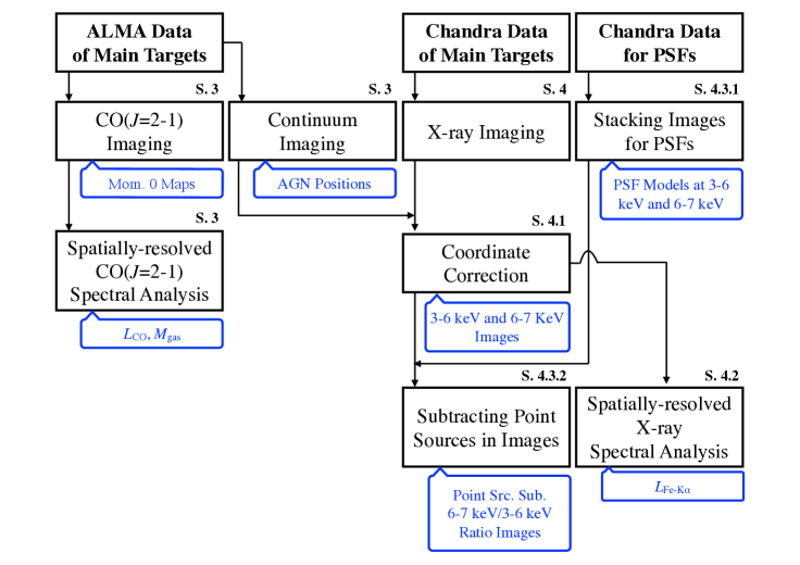
Figure 1: Flowchart for our main analyses. The numbers on the right shoulders of the black boxes indicate the sections where the corresponding analyses are explained. Additionally, the main products are indicated in the blue boxes.

Throughout this paper, we adopt standard cosmological parameters ($H_{0}$ = 70 km s^-1 Mpc^-1, $\Omega_{\rm m}$ = 0.3, $\Omega_{\Lambda}$ = 0.7). Unless otherwise stated, the uncertainties at the 1$\sigma$ confidence level are quoted.

Table 1: Target information

(1)	(2)	(3)	(4)	(5)	(6)	(7)	(8)	(9)	(10)
Number	Target name	R.A.	Decl.	$z$	$D$	pc/1″	$\Gamma$	$\log(N_{\rm H}$/cm${}^{-2})$	$\log[L_{\rm 20-50~{}keV}$/(erg/s)]
01	NGC 424	17.865170	-38.083467	0.0118	51.0	247	2.11	24.25	42.98
02	NGC 526A	20.976574	-35.065481	0.0191	83.0	402	1.43	22.01	43.21
03	NGC 612	23.490399	-36.493187	0.0305	133.7	648	1.71†	23.97†	43.80†
04	NGC 788	30.276933	-6.815881	0.0136	58.9	286	1.64	23.82	43.22
05	NGC 1052	40.269992	-8.255763	0.005	19.5	95	1.44	22.95	41.73
06	NGC 1068	40.669625	-0.013323	0.0038	12.7	62	1.9	25.0	42.39
07	NGC 1125	42.918575	-16.650651	0.011	47.5	230	1.9	24.21	42.49
08	NGC 1365	53.401529	-36.140430	0.0055	18.2	88	1.76	22.21	42.23
09	2MASX J0521-2521	80.255840	-25.362585	0.0426	188.4	913	2.6	22.92	43.23
10	NGC 2110	88.047406	-7.456249	0.0078	35.6	173	1.71	22.94	43.14
11	ESO 005-G004	91.422034	-86.631555	0.0062	22.4	109	1.64	24.18	42.23
12	Mrk 1210	121.024420	5.113847	0.0135	58.4	283	2.07	23.4	42.98
13	NGC 3081	149.873106	-22.826329	0.008	26.5	128	1.88	23.91	42.82
14	NGC 3393	162.097528	-25.162230	0.0125	54.0	262	2.22	24.4	42.57
15	NGC 4507	188.902654	-39.909359	0.0118	51.0	247	1.71	23.95	43.54
16	NGC 4945	196.364514	-49.468156	0.0019	8.1	39	1.38	24.8	42.62
17	ESO 323-077	196.608839	-40.414612	0.015	65.0	315	2.0	22.81	42.83
18	Mrk 463	209.012026	18.371872	0.0504	224.1	1086	1.64	23.81	43.35
19	NGC 5506	213.311996	-3.207678	0.0062	23.8	115	1.8	22.44	42.91
20	NGC 5643	218.169579	-44.174419	0.004	16.9	82	1.46	25.0	42.49
21	NGC 5728	220.599479	-17.253054	0.0093	30.6	148	1.5	24.14	42.87
22	NGC 6240	253.245380	2.400932	0.0245	106.9	518	1.95	24.25	44.25
23	Fairall 49	279.242649	-59.402303	0.0202	87.9	426	2.16	22.03	42.74
24	IC 5063	313.009841	-57.068772	0.0114	49.3	239	1.9	23.56	42.96
25	NGC 7130	327.081343	-34.951313	0.0162	70.2	340	2.03	24.22	42.52
26	NGC 7582	349.598514	-42.370433	0.0052	20.9	101	1.89	24.15	42.86

2 Sample selection

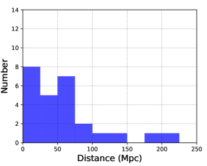
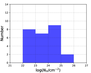
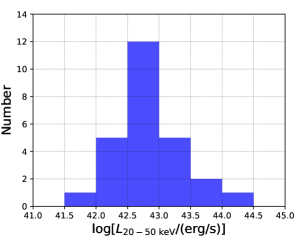
Figure 2: Distributions of the distances, the line-of-sight hydrogen column densities, and the absorption-corrected 20–50 keV luminosities of our sample.

To address our main question based on a sample that is not strongly biased by obscuration, we considered hard X-ray selected AGNs from the Swift/BAT AGN Spectroscopic Survey (BASS) project (Koss et al., 2017; Ricci et al., 2017a). This sample is based on the 70-month BAT catalog (Baumgartner et al., 2013), and provides not only precise nuclear X-ray properties (Ricci et al., 2017a), but also information obtained by follow-up observations at various wavelengths (e.g., Lamperti et al., 2017; Baek et al., 2019; Smith et al., 2020; Koss et al., 2021).

From the BASS Data Release 1 catalog, we first selected obscured AGNs with $\log(N_{\rm H}/{\rm cm}^{-2})>22$ at redshifts $\lesssim 0.05$, corresponding to $\approx$ 200 Mpc, suited to revealing extended X-ray emission. Line-of-sight obscuration makes it easier to detect extended faint emission. In addition, their proximity enables us to achieve high physical resolution. Then, we searched for their CO($J$=2–1) ALMA data, which were obtained with 12 m telescope arrays and were publicly available as of 2020 August. Next, we searched the ChaSeR web interface for Chandra archived ACIS data with a search radius of 1′. The radius was set to avoid poorer angular resolution due to the large offset between the aim-point and the targeted object. Here, we retained AGNs observed by either imaging or grating observations, but excluded objects if any of their observations were obtained with exposures less than 10 ks. To avoid confusion, we kept the objects that have at least one observation taken with an exposure larger than 10 ks, and considered all their available data even if some data were taken with exposures less than 10 ks. Finally, we checked the data quality, and, for example, we excluded Cen A, whose Chandra data are quite heavily affected by photon pileup around the nucleus. We then defined a sample consisting of 26 AGNs. The basic properties are summarized in Table 1, and some of them are presented as histograms in Figure 2.

We assessed the quality of all publicly available Chandra data as of 2020 August and considered only those that were not severely affected by either the photon pileup or particle events. We selected the highest resolution ALMA data for each target. However, for NGC 1068, we used the 2nd highest resolution data as the maximum recoverable scale (MRS) of the highest resolution less than 1″ cannot be used in conjunction with Chandra to discuss the properties of the circumnuclear gas, as is done for the other targets. To the contrary, the selected data have MRSs larger than 1″.3 and thus, retain good sensitivities to the angular scale of interest (e.g., $\sim$ 1″). Tables 2 and 3 summarize the Chandra and ALMA data adopted in this study.

As described in detail in Section 4.1, we define and separately discuss two types of regions: a central 2″ nuclear region and an external annular region of 2″–4″. The former and latter regions correspond to $\lesssim$ 100–600 pc and $\sim$ 100–1300 pc, respectively, for most of our AGNs (i.e., 19/26 or 73%). Hereafter, we refer to the two regions as the “nuclear” and “external” regions, respectively. Because of this definition, the physical scales of the regions do not match between nearby and distance objects. For example, the external regions of the nearest objects in our sample (e.g., $\sim$ 300–600 pc for a object at $D\sim$ 30 Mpc) can be within the nuclear regions of distant objects (e.g., $\lesssim$ 600 pc for a object at $D\sim$ 60 Mpc). However, our discussions are made while considering this fact as much as possible. Specifically, we discuss the relevance between Fe-K$\alpha$ and CO($J$=2–1) emission while extracting them from the same regions in Section 5.2.2, therefore, being unaffected by differences in object distance. Also, we limit our sample only to the nearest AGNs at distances $\lesssim$ 30 Mpc in Section 5.3.1.

Table 2: Chandra Data List

(1)	(2)	(3)	(4)	(5)
Number	Target name	ObsID	Grating	Exp.
01	NGC 424	3146	NONE	9.18
01	NGC 424	21417	NONE	15.28
02	NGC 526A	4376	HETG	28.68
02	NGC 526A	4437	HETG	29.07
03	NGC 612	16099	NONE	10.78
03	NGC 612	17577	NONE	24.73
04	NGC 788	11680	NONE	13.61
05	NGC 1052	385	NONE	2.34
05	NGC 1052	5910	NONE	59.20
06	NGC 1068	9148	HETG	79.57
06	NGC 1068	9149	HETG	88.73
06	NGC 1068	9150	HETG	41.08
06	NGC 1068	10815	HETG	19.07
06	NGC 1068	10816	HETG	16.16
06	NGC 1068	10817	HETG	32.65
06	NGC 1068	10823	HETG	34.54
06	NGC 1068	10829	HETG	38.44
06	NGC 1068	10830	HETG	42.90
07	NGC 1125	21418	NONE	53.15
08	NGC 1365	3554	NONE	14.61
08	NGC 1365	6868	NONE	14.61
08	NGC 1365	6869	NONE	15.54
08	NGC 1365	6870	NONE	14.55
08	NGC 1365	6871	NONE	13.36
08	NGC 1365	6872	NONE	14.62
08	NGC 1365	6873	NONE	14.64
08	NGC 1365	13920	HETG	88.53
08	NGC 1365	13921	HETG	108.20
09	2MASX J0521-2521	3432	NONE	14.86
10	NGC 2110	883	NONE	45.75
10	NGC 2110	3143	HETG	25.05
10	NGC 2110	3417	HETG	24.47
10	NGC 2110	3418	HETG	56.07
10	NGC 2110	4377	HETG	94.88
11	ESO 005-G004	21421	NONE	21.94
12	Mrk 1210	4875	NONE	10.41
12	Mrk 1210	9264	NONE	9.82
12	Mrk 1210	9265	NONE	9.41
12	Mrk 1210	9266	NONE	9.42
12	Mrk 1210	9267	NONE	9.80
12	Mrk 1210	9268	NONE	9.79
13	NGC 3081	20622	NONE	29.39

(1)	(2)	(3)	(4)	(5)
Number	Target name	ObsID	Grating	Exp.
14	NGC 3393	4868	NONE	29.33
14	NGC 3393	12290	NONE	69.16
14	NGC 3393	13967	HETG	176.78
14	NGC 3393	13968	HETG	28.06
14	NGC 3393	14403	HETG	77.72
14	NGC 3393	14404	HETG	56.68
15	NGC 4507	2150	HETG	138.20
15	NGC 4507	12292	NONE	39.60
16	NGC 4945	4899	HETG	77.37
16	NGC 4945	4900	HETG	95.60
16	NGC 4945	14984	NONE	128.76
16	NGC 4945	14985	NONE	68.73
17	ESO 323-077	11848	HETG	45.90
17	ESO 323-077	11849	HETG	118.14
17	ESO 323-077	12139	HETG	59.55
17	ESO 323-077	12204	HETG	67.34
18	Mrk 463	4913	NONE	49.33
18	Mrk 463	18194	NONE	9.57
19	NGC 5506	357	NONE	0.71
19	NGC 5506	1598	HETG	88.90
20	NGC 5643	5636	NONE	7.63
20	NGC 5643	17031	NONE	72.12
20	NGC 5643	17664	NONE	41.53
21	NGC 5728	4077	NONE	18.73
22	NGC 6240	1590	NONE	36.69
22	NGC 6240	6908	HETG	157.00
22	NGC 6240	6909	HETG	141.23
22	NGC 6240	12713	NONE	145.36
23	Fairall 49	3148	HETG	55.98
23	Fairall 49	3452	HETG	50.26
24	IC 5063	7878	NONE	34.10
24	IC 5063	21466	NONE	87.67
24	IC 5063	21467	NONE	26.93
24	IC 5063	21999	NONE	34.13
24	IC 5063	22000	NONE	15.64
24	IC 5063	22001	NONE	29.27
24	IC 5063	22002	NONE	43.87
25	NGC 7130	2188	NONE	38.64
26	NGC 7582	436	NONE	13.44
26	NGC 7582	2319	NONE	5.87
26	NGC 7582	16079	HETG	173.39
26	NGC 7582	16080	HETG	19.71

Table 3: ALMA Data

(1)	(2)	(3)	(4)	(5)	(6)	(7)	(8)
Number	Target name	Project code	Beam size	P.A.	MRS	Mosaic	rms
01	NGC 424	2017.1.00236.S	0″.11$\times$0″.09	1∘.4	1″.9	no	0.025
02	NGC 526A	2018.1.00538.S	0″.34$\times$0″.31	68∘.4	3″.7	no	0.037
03	NGC 612	2015.1.01572.S	0″.33$\times$0″.28	$-$75∘.4	3″.5	no	0.084
04	NGC 788	2018.1.00538.S	0″.41$\times$0″.30	65∘.3	4″.0	no	0.099
05	NGC 1052	2013.1.01225.S	0″.25$\times$0″.19	1∘.1	1″.9	no	0.048
06	NGC 1068	2016.1.00232.S	0″.34$\times$0″.28	1∘.4	2″.8	no	0.046
07	NGC 1125	2017.1.00236.S	0″.17$\times$0″.12	$-$69∘.7	2″.5	no	0.028
08	NGC 1365	2013.1.01161.S	0″.92$\times$0″.69	80∘.3	1″.9	yes	0.618
09	2MASX J0521-2521	2018.1.00699.S	0″.58$\times$0″.49	$-$74∘.4	5″.9	no	0.048
10	NGC 2110	2012.1.00474.S	0″.87$\times$0″.54	$-$1∘.3	1″.3	no	0.060
11	ESO 005-G004	2013.1.00623.S	2″.02$\times$1″.20	65∘.9	9″.3	no	0.218
12	Mrk 1210	2017.1.01439.S	0″.45$\times$0″.40	$-$88∘.7	4″.3	no	0.074
13	NGC 3081	2015.1.00086.S	0″.60$\times$0″.52	$-$1∘.4	5″.2	no	0.055
14	NGC 3393	2016.1.01553.S	0″.43$\times$0″.32	56∘.3	4″.6	no	0.064
15	NGC 4507	2018.1.00538.S	0″.34$\times$0″.33	63∘.2	3″.7	no	0.089
16	NGC 4945	2016.1.01279.S	0″.50$\times$0″.48	$-$3∘.5	4″.5	yes	0.071
17	ESO 323-077	2018.1.00538.S	0″.35$\times$0″.31	$-$73∘.7	3″.9	no	0.051
18	Mrk 463	2013.1.00525.S	0″.41$\times$0″.21	$-$0∘.9	1″.8	no	0.080
19	NGC 5506	2017.1.00236.S	0″.32$\times$0″.26	1∘.0	3″.6	yes	0.135
20	NGC 5643	2016.1.00254.S	0″.31$\times$0″.24	$-$50∘.0	1″.7	no	0.047
21	NGC 5728	2015.1.00086.S	0″.59$\times$0″.51	$-$1∘.3	5″.0	no	0.070
22	NGC 6240	2015.1.00370.S	0″.80$\times$0″.69	0∘.9	5″.0	no	0.247
23	Fairall 49	2017.1.00904.S	0″.19$\times$0″.13	$-$5∘.9	4″.1	no	0.070
24	IC 5063	2016.1.01279.S	0″.48$\times$0″.31	54∘.8	4″.0	yes	0.063
25	NGC 7130	2017.1.00255.S	0″.46$\times$0″.34	1∘.2	3″.7	no	0.029
26	NGC 7582	2016.1.00254.S	0″.16$\times$0″.12	$-$12∘.3	1″.3	no	0.028

3 ALMA data and analysis

The ALMA data were analyzed to produce continuum and CO($J$=2–1) images. The positions of our AGNs were determined based on the continuum images and were then used to mitigate systematic offsets of coordinates between ALMA and Chandra images by matching Chandra- and ALMA-determined AGN positions (Section 4.1). This is crucial to reliably compare ALMA and Chandra images. Additionally, the CO($J$=2–1) images were used to estimate spatially resolved gas masses.

We analyzed the ALMA data using the Common Astronomy Software Applications package (CASA; McMullin et al., 2007). For data reduction and calibration, we adopted the same CASA versions as those used in the quality verification by the ALMA Regional Center. After completing the above tasks, we uniformly used CASA ver. 5.6.1. for image reconstruction and to derive the physical values.

To produce images of the continuum emission, we first identified spectral channels free of any emission lines via the plotms task. For each target, a single image at a frequency is produced from the defined channels by tclean in the multi-frequency synthesis mode, with the Briggs weighting (robust = 0.5). For data obtained in a mosaic mode, we set gridder to mosaic. Alternatively, to produce a continuum-subtracted CO($J$=2–1) cube, we first determined the continuum level by fitting line-free channels with zeroth- or first-order functions, and subtracted it via the task uvcontsub. The product was then deconvolved using tclean with the same weighting as that used for continuum emission. Considering that velocity resolutions were different among the targets, we combined native bins to achieve resolutions of $\approx$ 10 km s^-1 for all, except for ESO 005-G009, becauase this source was originally observed at a larger native resolution of $\approx$ 20 km s^-1. Notably, some images were produced by adopting different parameters in the tclean task, such as that for robust, and/or by applying a mask for possible CO($J$=2–1) emitting regions. This is because the default setting yielded severe systematic residuals. Basic information of the ALMA data is summarized in Table 3.

Significant nuclear continuum emission was detected for all targets except for ESO 005-G004. While we were not able to detect nuclear continuum emission of NGC 1365 by combining all three data available through project 2013.1.01161.S, we successfully detected it by considering only the highest-resolution data with a beam size of 0″.19$\times$0″.21. For those with significant detections, we estimated the AGN positions by applying the imfit CASA task to probable AGN continuum components with reference to the literature, NED and SIMBAD. For two merger systems, NGC 6240 and Mrk 463, we found two bright nuclei for each. NGC 6240 showed south and north nuclei, and their positions were close to those of X-ray nuclei (e.g., Komossa et al., 2003; Puccetti et al., 2016; Treister et al., 2020). As the southern one was apparently brighter, we adopted it as the main AGN. While Mrk 463 showed east and west nuclei, known to have intrinsically similar X-ray luminosities (e.g., Treister et al., 2018; Yamada et al., 2018), the eastern nucleus was apparently brighter in both the X-ray and millimeter bands. Thus, the eastern nucleus was adopted as the main AGN. Because no significant emission was observed from ESO 005-G004, we adopted an optical AGN position from the NED. The determined and adopted AGN positions are summarized in Table 1.

Regarding the nondetection of ESO 005-G004, that may be partly due to its low X-ray luminosity ($\sim$ $10^{42}$ erg s^-1). If a correlation between X-ray and millimeter luminosities proposed in some studies (e.g., Behar et al., 2015, 2018) is valid for this object, its 100 GHz luminosity may be as low as $\approx 3\times 10^{38}$ erg s^-1. By considering the millimeter spectral shapes of nearby AGNs unveiled by Inoue & Doi (2018), an expected luminosity at $\sim$ 200 GHz is $\sim 10^{38}$ erg s^-1. As the achieved sensitivity for continuum emission is $\sim$ $2\times 10^{-4}$ Jy beam^-1 and a luminosity of $10^{38}$ erg s^-1 corresponds to $\sim$ 5$\sigma$, the nondetection is thus unsurprising.

We extracted CO($J$=2–1) spectra from the nuclear ($<$ 2″) and external ($r=$2″–4″) regions centered at the AGN positions. Significant CO($J$=2–1) emission was found for 22 targets in both regions. As an example, Figure 3 shows the spectra of NGC 1068 for three different extraction regions, and all the spectra are shown in Appendix E. Throughout this paper, velocities are denoted in the optical convention (i.e., speed of light $\times$ redshift). Uniquely, the nuclear spectrum of NGC 1052 was dominated by absorption. Specifically, Kameno et al. (2020) confirmed that the absorption was concentrated within $\approx$ 0.″5 of the center, which is consistent with our finding. The remaining three AGNs (NGC 424, NGC 526A, and Mrk 463) showed no significant emission in either the nuclear or external regions.

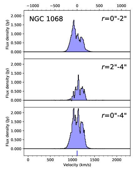
Figure 3: Spectra around CO($J$=2–1) emission taken for NGC 1068. From top to bottom, they were extracted from a circle of radius 2″, an annulus of radius 2″–4″, and a circle of radius 4″. Based on the spectrum from the 4″ circle, a channel range to calculate the flux was defined (i.e., blue shaded regions). The centroid of the emission was derived based on the range and is indicated by the blue vertical line in the bottom panel. The top and bottom scales denote the relative velocity to the line centroid and the velocity in the optical convention, respectively. The latter velocity at the line centroid is thus a CO($J$=2–1)-estimated systematic velocity of the galaxy. The spectra of all targets can be seen in Appendix E.

We adopted a nonparametric method to derive CO($J$=2–1) fluxes. This is because for a non-negligible number of targets, the spectral shapes of the CO($J$=2–1) emission were jagged and could not be reproduced by a few Gaussian functions (Figure 3 and Appendix E). We first extracted a spectrum from the 4″-radius circular region centered at each AGN position, and then defined contiguous channels around the systemic velocity where the emission was significant above 1$\sigma$. For example, a defined channel range is shown by blue shaded areas in Figure 3. Such areas are also denoted in Appendix E. Finally, we integrated flux densities over the defined channel range. Note that NGC 424 was exceptionally treated by using its 2″-radius circular region, as its CO($J$=2–1) emission was slightly smeared out in the 4″-radius spectrum.

Table 4 summarizes the CO($J$=2–1) luminosities, calculated according to Solomon & Vanden Bout (2005), and their errors. The errors consider the statistical error and conventional 10% systematic error, originating from uncertainty in the absolute flux calibration. As the nuclear spectrum of NGC 1052 was dominated by the absorption, we listed the sum of the 1-$\sigma$ uncertainty and the absorption strength as the upper limit of the CO($J$=2–1) luminosity. In addition to NGC 1052, other AGNs whose CO($J$=2–1) emission is significantly absorbed can be expected. However, the effect would be negligible (i.e., $\sim$ 0.1 dex). To confirm this, we performed a detailed analysis of the spectrum taken from the center of NGC 4945, the details of which are presented in Appendix A. This AGN was selected because its nuclear 2″ spectrum can be most easily affected by absorption owing to its proximity ($\sim 8$ Mpc), except for NGC 1052. This is also suggested from previous reports on clear absorption lines due to HCN($J$=1–0) and HCO⁺($J$=1–0) (e.g., Henkel et al., 2018).

Table 4 lists the molecular gas masses derived from the CO($J$=2–1) luminosities. We adopted a CO($J$=1–0)-to-CO($J$=2–1) brightness temperature ratio of 1.4 and an $\alpha_{\rm CO}$ conversion factor of 0.8 $M_{\odot}$(K km s^-1 pc²)^-1 (Sandstrom et al., 2013). Throughout this paper, we do not discuss the absolute values of the gas masses. Therefore, a different choice of ratio or conversion factor does not have any effect on our discussion and conclusion.

As the final analysis of the ALMA data, we produced the moment 0 (intensity) maps of the CO($J$=2–1) emission. For each data cube, zeroth moments were calculated over a 1000 km s^-1 range centered at the centroid of the emission. The centroid was computed based on the spectrum obtained from the 4″-radius region. As NGC 6240 showed very broad CO($J$=2–1) emission, we considered a 2000 km s^-1 width. All the moment 0 images are shown in Appendix F.

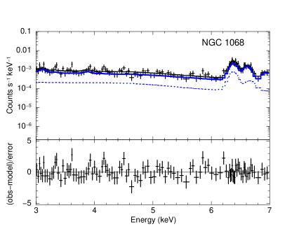
Figure 4: (Left) X-ray spectrum taken from the circle of radius 2″ centered at the AGN position of NGC 1068. The upper window shows the observed data (black crosses) and the best-fit model (black solid line), and the lower window shows the residuals. (Right) X-ray spectrum taken from the central annulus of radius 2″–4″ for NGC 1068. The spectrum is reproduced by considering essentially two components: one is from the extracted 2″–4″ region (blue solid line), and the other is from the central point source extended by the PSF (blue dotted line).

Table 4: CO($J$=2–1) Line Luminosities and Derived Gas Mass

(1)	(2)	(3)	(4)	(5)	(6)	(7)	(8)	(9)	(10)
Number	Target name	$L^{\rm nuc}_{\rm CO}$	$\Delta L^{\rm nuc}_{\rm CO}$	$M^{\rm nuc}_{\rm gas}$	$\Delta M^{\rm nuc}_{\rm gas}$	$L^{\rm ext}_{\rm CO}$	$\Delta L^{\rm ext}_{\rm CO}$	$M^{\rm ext}_{\rm gas}$	$\Delta M^{\rm ext}_{\rm gas}$
01	NGC 424	6.78	0.78	7.59	0.87	$<0.76$	…	$<0.85$	…
02	NGC 526A	$<0.43$	…	$<0.48$	…	4.92	0.99	5.51	1.11
03	NGC 612	498	52	557	58	684	73	766	81
04	NGC 788	16.8	2.1	18.8	2.3	8.3	2.1	9.3	2.4
05	NGC 1052	$<0.17$	…	$<0.19$	…	$<0.01$	…	$<0.01$	…
06	NGC 1068	33.6	3.4	37.7	3.8	17.9	1.8	20.0	2.0
07	NGC 1125	22.7	2.3	25.4	2.6	4.63	0.79	5.18	0.88
08	NGC 1365	11.3	1.2	12.7	1.3	63.0	6.3	70.6	7.1
09	2MASX J05210136-2521450	2150	220	2400	240	234	24	262	27
10	NGC 2110	11.0	1.1	12.3	1.2	9.73	0.99	10.9	1.1
11	ESO 005-G004	1.94	0.20	2.17	0.22	4.03	0.41	4.51	0.46
12	Mrk 1210	15.6	1.6	17.4	1.8	29.4	3.0	32.9	3.4
13	NGC 3081	9.31	0.93	10.4	1.0	2.96	0.31	3.31	0.35
14	NGC 3393	14.8	1.6	16.5	1.7	24.5	2.6	27.4	2.9
15	NGC 4507	70.4	7.1	78.8	7.9	43.1	4.6	48.2	5.1
16	NGC 4945	56.6	5.7	63.4	6.3	69.4	6.9	77.8	7.8
17	ESO 323-077	238	24	266	27	332	33	372	37
18	Mrk 463	466	50	522	56	$<28$	…	$<31$	…
19	NGC 5506	38.9	3.9	43.6	4.4	22.8	2.4	25.5	2.7
20	NGC 5643	40.2	4.0	45.0	4.5	36.8	3.7	41.2	4.1
21	NGC 5728	36.7	3.7	41.1	4.1	35.6	3.6	39.9	4.0
22	NGC 6240	6540	650	7320	730	2510	250	2810	280
23	Fairall 49	386	39	432	44	151	17	169	19
24	IC 5063	34.0	3.4	38.1	3.8	17.6	1.9	19.7	2.1
25	NGC 7130	936	94	1050	110	341	34	382	38
26	NGC 7582	120	12	134	13	60.4	6.0	67.6	6.8

4 Chandra data and analysis

4.1 Data Reduction

We analyzed Chandra data with two aims: (i) to measure spatially resolved Fe-K$\alpha$ fluxes and (ii) to map the Fe-K$\alpha$ emission. Throughout the analyses of the Chandra data, the CIAO 4.12 package was used along with CALDB version 4.9.1. Raw data obtained from ChaSeR were reprocessed in a standard manner using chandra_repro. Then, we filtered events in a period when a flare of background counts, likely due to cosmic rays, was observed. Some of our targets were bright enough to cause pileup, making it difficult to recover the intrinsic flux. Thus, we discarded data where the pileup with a fraction of 5% extended over 2″ around a nuclear X-ray peak. The fraction was estimated from the observed counts per read time using the CIAO task pileup_map. The 2″ radius was selected so that we could extract the nuclear spectra that were unaffected by the photon pileup.

As first mentioned in Section 2, we defined the nuclear region of 2″ and the external region of 2″–4″. The 2″ outer radius of the nuclear region was selected as a significant fraction of the Chandra data were affected by the photon pileup within $\sim$ 1″, but the effect did not frequently extend over 2″. Thus, 2″ was a reasonable optimization that allowed us to extract nuclear spectra from either a circular 2″ region or an annular 1″–2″ region, depending on the degree of the pileup effect. With this determination, we measured the nuclear and external CO($J$=2–1) fluxes discussed in Section 3.

As the final data reprocessing step, we corrected the systematic offsets between the coordinates of the Chandra and ALMA images. In each Chandra image, we first calculated the centroid of the nuclear X-ray photons in the 3–7 keV band, where nuclear emission was likely to be dominant. Then, we modified the coordinates of the Chandra image such that the X-ray centroid matched the AGN position determined from the ALMA continuum image. Notably, the positional offsets before the adjustment were generally less than 0″.5.

4.2 Spatially resolved X-ray Spectroscopy

We derived Fe-K$\alpha$ fluxes in both the nuclear ($r<$ 2″) and external ($r$ = 2″–4″) regions. For the nongrating data, we estimated the fluxes simply based on the spectra extracted from the two regions. If the pileup effect was severe within 1″, we adopted an annulus of 1″–2″ instead of the circular region. If there were more than one observation, we combined the spectra into a single spectrum. Response files for the nuclear and external spectra were produced by assuming a point source and an extended source, respectively. For the grating data, we used 1st-order HEG spectra to measure nuclear Fe-K$\alpha$ fluxes because they are not affected significantly by the pile-up. Notably, the contamination from extended or surrounding sources is expected to be not severe given their creation process. For the external components, we extracted spectra from annuli of 2″–4″  based on the 0th-order image. If multiple spectra were available for each target, they were merged into one. All the extracted spectra were binned to have at least one count per bin. In almost the same manner as adopted for the imaging observations, their response files were created.

As an example, Figure 4 shows the spectra of NGC 1068 taken from its nuclear and external regions together with the best-fit models, detailed in the following paragraphs. Appendix 21 summarizes the corresponding figures for all our targets.

The nuclear spectra in the 3–7 keV band were fitted with C-statistics. This energy range was selected because we were not interested in soft X-ray components, such as thermal emission due to stellar activity, a soft-X-ray excess linked to the accretion disk, scattered nuclear light, and emission from hot extended cluster gas. When both imaging and grating data were available for a single object, we fitted the two spectra jointly without merging them. As our fiducial model, we employed a phenomenological model of constant*(zTBabs*zpowerlw + zgauss + zgauss) in XSPEC terminology. When imaging and grating data were available, the constant model was allowed to vary by 10% to account for any calibration uncertainty in the normalization of the different spectra. Then, we considered an absorbed transmitted power-law emission from the central X-ray corona as zTBabs*zpowerlw, and two Gaussian functions (i.e., zgauss + zgauss) to reproduce the Fe-K$\alpha$ and Fe-K$\beta$ lines at 6.40 and 7.06 keV. Given the low photon statistics of the majority of the spectra, we fixed the power-law photon indices at those determined based on broadband X-ray spectra ($\approx$ 0.5–200 keV) by Ricci et al. (2017a), except for NGC 612. The photon index of NGC 612 was estimated to be 1.07 in the hard X-ray catalog (Ricci et al., 2017a), which is particularly low and could be the result of heavy obscuration and low signal-to-noise ratio. Thus, we adopted a more likely value of $\Gamma=$ 1.71, which was derived based on a broadband spectrum in Ursini et al. (2018). As long as we had a grating spectrum, we retained the linewidth of Fe-K$\alpha$ as a free parameter and tied it to the width of Fe-K$\beta$. The other remaining free parameters were the absorbing hydrogen column density and the normalizations of the power-law and emission lines. The atomic abundance was set to the solar value determined by Wilms et al. (2000). If non-negligible residuals were found after fitting the fiducial model, according to their shape, we considered additional components, such as line emission from highly ionized iron atoms (e.g., Fe xxv and Fe xxvi), an unabsorbed power-law component representing scattered emission, and high-temperature ($\sim$ 1 keV) thermal emission. If any of these components improved the fit at the 90% confidence level (i.e., $\Delta C>$ 2.71), we incorporated it into the model.

The external spectra in the 3–7 keV band were fitted by adopting C-statistics. As our fiducial model for the emission from external regions, we considered constant*(pexrav + zgauss). The first constant was employed to absorb the calibration uncertainty between the grating and imaging spectra found in the fits to the nuclear spectra and was accordingly fixed. If either the grating or imaging spectrum was available, it was removed. The last two terms account for a reflection continuum (Magdziarz & Zdziarski, 1995) and Fe-K$\alpha$ emission. In addition to these components, we considered the contributions from the nuclear sources determined previously. These contributions are usually not negligible. As with the analyses for the nuclear spectra, we added certain components, provided that they improved the fits.

The derived Fe-K$\alpha$ luminosities in both the nuclear and external regions ($L^{\rm nuc}_{\rm Fe-K\alpha}$ and $L^{\rm ext}_{\rm Fe-K\alpha}$) are summarized in Table 5. As shown in the table, we detected Fe-K$\alpha$ emission above 1$\sigma$ from all but two (Fairall 49 and 2MASX J0521-2521) on the nuclear scale ($r<$ 2″) and nine objects (i.e., NGC 526A, NGC1068, NGC 2110, NGC 3393, NGC 4945, NGC 5643, NGC 6240, NGC 7130, and NGC 7582) on the external scale ($r=$ 2″–4″). Using 20–50 keV luminosities ($L_{\rm 20-50~{}keV}$) determined based on BAT spectra averaged over 70 months (Ricci et al., 2017a; Ursini et al., 2018), we calculated the ratios of $L^{\rm nuc}_{\rm Fe-K\alpha}/L_{\rm 20-50~{}keV}$ and $L^{\rm ext}_{\rm Fe-K\alpha}/L_{\rm 20-50~{}keV}$. These can be used as a proxy of the solid angle of gas irradiated by hard X-ray emission. Compared with the Fe-K$\alpha$ equivalent width (EW), the ratios are less affected by the absorption of underlying continuum emission. Additionally, because we adopt luminosities derived from the long-term-averaged spectra, they are less subject to short-time variability of continuum emission that is not associated with the narrow Fe-K$\alpha$ emission line. Here, we note two clear merging systems of NGC 6240 and Mrk 463 in the X-ray band (e.g., Komossa et al., 2003; Bianchi et al., 2008). The central 2″ region of NGC 6240 encompasses bright double nuclei. Thus, the Fe-K$\alpha$ luminosity includes both contributions. As the 20–50 keV luminosity was also calculated as the sum of the nuclei (Ricci et al., 2017a), the line-to-continuum luminosity ratio was calculated consistently. Regarding Mrk 463, the second nucleus is located at $\sim$ 4″ from the primary nucleus. Thus, the Fe-K$\alpha$ luminosity on the external scale was derived from the spectrum between 2″ and 4″, from which a 1″ circular region around the second nucleus was excluded.

Table 5: Fe-K$\alpha$ Luminosities

(1)	(2)	(3)	(4)	(5)	(6)	(7)	(8)
Number	Target name	$L^{\rm nuc}_{\rm Fe-K\alpha}$	$\Delta L^{\rm nuc}_{\rm Fe,low}$	$\Delta L^{\rm nuc}_{\rm Fe,upp}$	$L^{\rm ext}_{\rm Fe-K\alpha}$	$\Delta L^{\rm ext}_{\rm Fe,low}$	$\Delta L^{\rm ext}_{\rm Fe,upp}$
01	NGC 424	4.74	0.78	0.87	$<7.0$	…	…
02	NGC 526A	19.1	7.8	8.2	51	45	56
03	NGC 612	13.3	2.7	2.9	$<34$	…	…
04	NGC 788	3.1	1.5	1.6	$<62$	…	…
05	NGC 1052	0.55	0.18	0.19	$<0.48$	…	…
06	NGC 1068	0.86	0.05	0.05	5.89	0.71	0.77
07	NGC 1125	1.47	0.26	0.28	$<2.0$	…	…
08	NGC 1365	0.50	0.09	0.10	$<0.15$	…	…
09	2MASX J05210136-2521450	$<28$	…	…	$<94$	…	…
10	NGC 2110	8.82	1.84	0.93	46.0	8.9	8.3
11	ESO 005-G004	0.96	0.14	0.16	$<3.70$	…	…
12	Mrk 1210	14.9	4.5	5.0	$<5.2$	…	…
13	NGC 3081	6.0	1.7	1.9	$<1.2$	…	…
14	NGC 3393	1.61	0.22	0.23	12.8	3.9	4.5
15	NGC 4507	18.9	1.3	1.3	$<10.5$	…	…
16	NGC 4945	0.17	0.01	0.01	2.95	0.29	0.29
17	ESO 323-077	5.7	1.1	1.2	$<19$	…	…
18	Mrk 463	8.8	3.2	3.6	$<100$	…	…
19	NGC 5506	4.74	1.15	0.79	$<2.2$	…	…
20	NGC 5643	0.52	0.03	0.04	1.57	0.76	0.88
21	NGC 5728	2.21	0.43	0.47	$<3.8$	…	…
22	NGC 6240	18.2	1.1	1.3	98	22	24
23	Fairall 49	$<4.4$	…	…	$<26$	…	…
24	IC 5063	9.1	1.7	1.7	$<1.8$	…	…
25	NGC 7130	1.71	0.43	0.50	12	11	18
26	NGC 7582	1.02	0.24	0.17	1.6	1.4	1.7

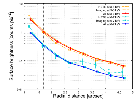
Figure 5: Radial profiles of surface brightness (counts pix^-2) as a function of radial distance (arcsec) for different energy bands (3–6 and 6–7 keV) and types of data (imaging and grating data). The profiles at 6–7 keV are shifted downward by 0.5 dex for clarity. In addtion, those solely from the HEG and imaging data are slightly shifted around their averaged profiles in the horizontal direction. Note that the left-most points correspond to those at 3.5 pixel from the central pixels.

4.3 X-ray Imaging

The Chandra data were further used to reveal the distributions of extended Fe-K$\alpha$ emission at $\approx$ 0″.5, which are comparable to those of the ALMA data. For this analysis, we first empirically constructed point spread functions (PSFs) in the 3–6 and 6–7  keV bands (Section 4.3.1). Then, we modeled point source images based on the PSFs and subtracted them from the observed ones (Section 4.3.2).

We note that although one popular method to obtain a PSF is to perform a Monte Carlo simulation with MARX, we found that for bright objects, there seems to be a significant difference between the simulated and observed profiles. This discrepancy cannot be ignored in bright objects. Therefore, we finally decided to adopt an empirical approach.

4.3.1 Construction of PSF models of Chandra

To construct the PSFs, we first compiled Chandra data of bright galactic X-ray sources and then stacked their observed images in the 3–6 and 6–7 keV bands. We searched ChaSeR for ACIS data of galactic X-ray sources listed in all-sky catalogs created by Monitor of All-sky X-ray Image (MAXI; Kawamuro et al., 2018; Hori et al., 2018). The galactic X-ray sources included those classified as ALGOL Star, CV, Dwarf Nova, high-mass X-ray binary, low-mass X-ray binary, Nova, Pulsar, RS CVn Star, Rotationally variable Star, Spectroscopic binary, Star, Symbiotic Star, Variable Star, and X-ray binary. The catalogs were suitable because the energy band of 4–10 keV covered the band of interest and provided one of the largest samples of bright X-ray sources. At this point, we excluded objects known to have bright X-ray extended emission, such as an object with a highly extended jet and a system consisting of double X-ray nuclei (e.g., Circinus X-1 and CH Cyg). In addition, the effect of X-ray halos produced by dust scattering (e.g., Predehl & Schmitt, 1995) is likely negligible, as discussed in the last paragraph of this section. Even after these selections and considerations, there may have remained X-ray sources that showed emission resolvable by Chandra but were difficult to identify by visual inspection. Although such objects expand our empirical PSFs, the expanded PSFs avoid the overestimation of extended emission, enabling conservative discussion of the presence of extended emission.

For PSF construction, only ACIS-S imaging and ACIS-S/HETG data were selected to match the data of our original targets. We excluded data affected by photon pileup. Furthermore, to avoid noisy and nonmeaningful data, we only used 10 data with the highest net-source counts at 3–7 keV within 5″ around the targeted X-ray sources. The 5″ radius was selected to cover the outer 4″ radii of the external regions. To verify the agreement between the PSFs of the grating and nongrating data, we eventually analyzed 10 data for each observation mode, that is, 20 data in total. Table 6 summarizes the information of the 20 data.

The selected data were reprocessed in the same manner as those used for our main targets. Then, for each data, we defined multiple concentric annuli with 0″.49 width (i.e., the ACIS-S native resolution) centered at the AGN position, producing the radial profiles of surface brightness in units of counts pix^-2 at 3–6 and 6–7 keV. In each dataset of the imaging and the grating, we calculated weighted means of the profiles of the two bands. Figure 5 shows the obtained profiles of the surface brightness normalized to 1 at 3.5 pixels from the centers. At pixels below 1″.5, the grating profiles show slightly lower surface brightness than the imaging profiles. This is because of the stronger photon pileup in the grating observations. The grating observation is less affected by the pileup, but the stronger pileup was due to the observations of the very bright sources. On the contrary, at larger radii beyond $\sim$ 1″.5, the profiles obtained from the imaging and grating observations were in agreement in both energy bands. Although we can see a bump for the imaging 6–7 keV data in the range of 3″–5″, which can be ascribed to poor count statistics, it is compatible with the grating data within 2$\sigma$. Finally, we derived a single PSF model for each energy band by taking the average of the imaging and grating profiles. In the following analysis, however, each PSF within a radius of 1″.5 was ignored, given that the pileup likely disturbed the PSF. A similar empirical method was adopted by Andonie et al. (in prep.) to produce PSF models.

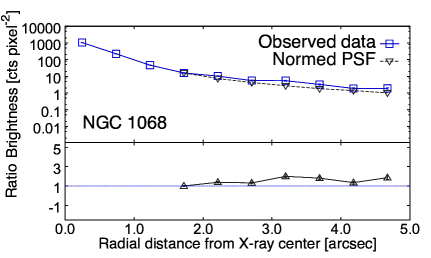
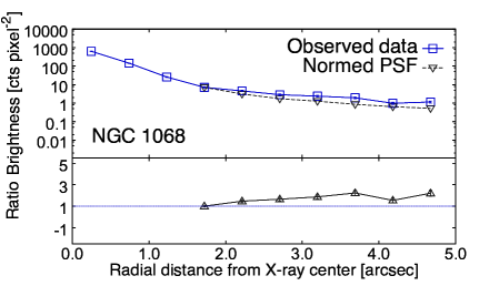
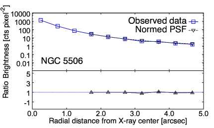
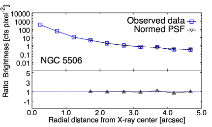
Figure 6: Top: Comparisons of observed profiles and those modeled by assuming a point source at 3–6 keV (left) and 6–7 keV (right) for NGC 1068. The ratios are shown in the lower panels. Bottom: Same figures for NGC 5506, one of the brightest AGNs in our sample.

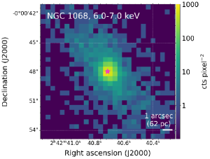
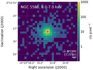
Figure 7: From left to right, 3–6 and 6–7 keV images and the ratios of 6–7 and 3–6 keV images from which nuclear point source emission is subtracted. The color bars in the 1st and 2nd columns indicate counts per pixel², and those in the 3rd one indicate count ratios. North is up and east is left. The upper and lower panels show images of NGC 1068 and NGC 5506, respectively. The central magenta stars indicate the AGN positions. Circles from the inner to outer ones in the right panels denote the 3.5 pixel at which the PSF is normalized to model a nuclear point source, a 2″ radius, and a 4″ radius. Note that no ratios in the central $\sim$ 2″ are shown because the modeled emission from the central point sources are subtracted.

It can be expected that the PSF depends on the energy, but the effect is negligible. This is inferred from the fact that the 3–6 keV profiles, dominated by softer photons, are close to those at 6–7 keV. A Chandra team also reported a supportive result that showed almost the same profiles between the 4.5 and 6.4 keV bands.

Finally, we suggest that the impact of dust-scattering X-ray halos on the PSF model is insignificant. For this suggestion, we compared PSF models created for two subsamples consisting of objects with low column densities below $10^{21}$ cm^-2 and those with high column densities above $10^{21}$ cm^-2 (Table 6). We then obtained a supportive result that the PSF models agreed within 1$\sigma$.

4.3.2 Point-Source-Subtracted X-ray Images

Using the PSF models obtained in Section 4.3.1, we produced point-source-subtracted images at 3–6 and 6–7 keV. From the reprocessed data of the main targets, we produced images in the two bands at an ACIS-S native resolution of 0″.49. If multiple data were available for a single object, the images were stacked into one. Then, for each image, we derived photon counts at 3.5 pixels from the AGN position and modeled a point source image by renormalizing the PSF model in an appropriate energy band to match the photon counts.

In Figure 6, we representatively show the observed radial profiles and those of the modeled point source images for NGC 1068 and NGC 5506. The former is adopted to show a case where clear extended emission is present, and the latter is an example showing good agreement between the observed and modeled profiles. All the figures are shown in Appendix C, and it can be seen that the observed profiles are generally not overestimated by those of the modeled point source images, suggesting the success of our modeling. Then, we subtracted the models from the observed images and calculated the ratios between the 6–7 and 3–6 keV images to indicate the sites with bright Fe-K$\alpha$ emission. Note that in some objects, emission from highly ionized iron atoms also contribute to the ratio (e.g., NGC 1068, NGC 4945, and NGC 6240, as inferred from the spectra in Appendix 21). Here, to avoid extreme ratios due to very low denominator, or low counts in the 3.0–6.0 keV image, we excluded pixels with counts smaller than 2. This criterion corresponds approximately to the 1$\sigma$ level for a mean value of zero counts (Gehrels, 1986). The ratio images were then smoothed with a Gaussian kernel with a full width at half maximum of 1″.0. Figure 7 shows the ratio images created for NGC 1068 and NGC 5506.

Notably, NGC 6240 hosts two bright nuclei that are quite close ($<$ 1″), and it was difficult to estimate their PSF normalizations accurately. However, the 3–6 keV, 6–7 keV, and ratio images were created for completeness in the same manner as adopted for the others. Therefore, in this study, we do not discuss the obtained images in detail. Detailed imaging analyses can be found in Fabbiano et al. (2020).

Table 6: Data for Empirical PSF Construction

(1)	(2)	(3)	(4)
Target name	ObsID	Grating	Exp.
HD 110432	9947	HETG	139.49
AO PSC†	1898	HETG	98.50
4U 1626$-$67†	3504	HETG	94.81
AM HERCULIS†	3769	HETG	91.46
4U 1323-619	13721	HETG	79.00
XTE J1710-281	12468	HETG	73.31
XTE J1710-281	12469	HETG	73.30
NGC 1851†	18759	HETG	62.57
4U 1908+075	5477	HETG	49.00
4U 1907+09	21123	HETG	41.28
SAX J2103.5+4545	15780	NONE	45.41
NGC 6652†	12461	NONE	45.32
MAXI J0556-332†	14227	NONE	18.20
MAXI J1659-152	12441	NONE	18.15
MAXI J0556-332†	14429	NONE	13.67
NGC 6652†	18987	NONE	10.04
1RXS J045707.4+452751	3878	NONE	4.93
GRO J1008-57	14639	NONE	4.60
KS 1947+300	14647	NONE	4.60
4U 0728-25	14636	NONE	4.60

5 Discussion

Based on the results obtained in Sections 3 and 4, we address the main question, what impact does the hard X-ray irradiation have on the ISM and on star formation?. In the first half of this section (Sections 5.1 and 5.2), we focus on the external regions. Then, in the second half (Section 5.3), we focus on the nuclear regions.

5.1 Origin of extended Fe-K$\alpha$ emission

As reported in Section 4.2, Fe-K$\alpha$ emission was detected in the external regions of nine AGNs above 1$\sigma$. More reliably, six of them showed Fe-K$\alpha$ emission above 2$\sigma$ (i.e., NGC 1068, NGC 2110, NGC 3393, NGC 4945, NGC 5643, and NGC 6240). The luminosity ratios between the extended and nuclear Fe-K$\alpha$ emission are at most 0.1 (Figure 8). Thus, a large fraction of the Fe-K$\alpha$ emission originates from regions within a radius of $\sim$ 2″, corresponding to 100–600 pc for the majority of our targets (i.e., 19/26).

Although the extended Fe-K$\alpha$ emission is faint, its detailed study suggests the potential effect of hard X-ray irradiation on the ISM. We thus first discuss the following four conceivable mechanisms as the origin of the spatially extended Fe-K$\alpha$ emission: (1) This is the result of the Thomson scattering of Fe-K$\alpha$ photons produced by dense nuclear material (e.g., the putative torus; Fabbiano et al. 2017). (2) This is caused by the collisional ionization of Fe atoms by cosmic rays including electrons and ions (e.g., Valinia et al., 2000; Yusef-Zadeh et al., 2002, 2007). (3) The fluorescent X-ray emission following photoionization by high-energy X-ray photons above 7.1 keV produced by the AGN (e.g., Koyama et al., 2007; Nobukawa et al., 2010; Ponti et al., 2010). (4) The sum of contributions from multiple high-mass X-ray binaries (e.g., Torrejón et al., 2010).

In Section 5.1.1, we test the first scenario. Then, we discuss the next two scenarios in Section 5.1.2. Finally, the fourth idea is examined in Section 5.1.3. Following these discussions, we suggest that the detected Fe-K$\alpha$ emission can be explained based on the third scenario (i.e., AGN photoionization).

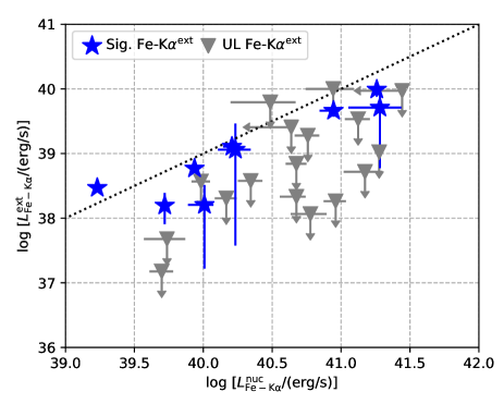
Figure 8: Scatter plot of Fe-K$\alpha$ luminosities derived from the nuclear and external regions. The dotted line is drawn where the ratio is 0.1. AGNs with significant detection and upper limits (UL) for Fe-K$\alpha$ emission in their external regions are indicated by blue stars and gray triangles, respectively.

5.1.1 Thomson Scattering of Nuclear Fe-K$\alpha$ Photons?

We first test the Thomson scattering scenario. The fraction of Thomson scattered light compared to direct emission (scattering fraction or $f_{\rm scat}$) has been well estimated for obscured AGNs using broadband X-ray spectroscopy (e.g., Bianchi & Guainazzi, 2007; Noguchi et al., 2010; Kawamuro et al., 2016a, b; Ricci et al., 2017a; Gupta et al., 2021). If the external Fe-K$\alpha$ emission is also the result of scattering, its luminosity with respect to primary X-ray emission ($L^{\rm ext}_{\rm Fe-K\alpha}/L_{\rm X}$), a proxy for the solid angle of gas seen from the nucleus, should correlate with the scattering fraction. To assess the correlation, we took the scattered fractions of our sample from Ricci et al. (2017a) (see also Gupta et al., 2021), except for NGC 612, for which we referred to Ursini et al. (2018).

Figure 9 shows a scatter plot of $\log(f_{\rm scat}/\%)$ and $\log(L^{\rm ext}_{\rm Fe-K\alpha}/L_{\rm 20-50~{}keV})$, and no clear correlation is seen between these two parameters. To confirm this, we derive the $p$-value ($P$) and the Spearman rank coefficient ($\rho_{\rm S}$) using a bootstrap method. Following previous works (e.g., Ricci et al., 2014; Gupta et al., 2021), we draw a number of datasets based on the 26 real data, considering their uncertainties. For data with upper and lower errors, we randomly draw values from a Gaussian distribution whose mean and standard deviation are set to the best value and its 1$\sigma$ error, respectively. If the upper and lower 1$\sigma$ errors are asymmetric, we simply use the mean of the two. For the data that only have an upper limit, we use a uniform distribution between zero and the upper limit. Any drawn datasets including unphysical negative values were discarded. For each dataset, we compute the $p$-value and the Spearman rank coefficient using a Python program of spearmnr. We then fit the data using a relation of the form $\log Y=a+b\times\log X$, using the ordinary least-squares bisector regression fitting algorithm (Isobe et al., 1990). Finally, we consider the 16th and 84th percentiles of the distributions of the parameters ($P$, $\rho_{\rm S}$, $a$, and $b$) as their lower and upper limits, respectively. For $X$ = $(f_{\rm scat}/\%)$ and $Y$ = $(L^{\rm ext}_{\rm Fe-K\alpha}/L_{\rm 20-50~{}keV})$, we draw $\approx$ 10000 datasets and find $P=0.65^{+0.25}_{-0.29}$, indicating no correlation. Finally, we could not obtain evidence supporting the Thomson scattering scenario as the general origin of the external Fe-K$\alpha$ emission. However, it should be noted that there may be objects such as ESO 428-G014 (e.g., Fabbiano et al., 2017, 2018a, 2018b), in which the extended Fe-K$\alpha$ is due to Thomson scattering.

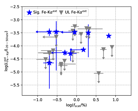
Figure 9: Scatter plot of the fraction of scattered X-ray light ($f_{\rm scat}$) and the Fe-K$\alpha$-to-continuum luminosity ratio ($L^{\rm ext}_{\rm Fe-K\alpha}$/$L_{\rm 20-50~{}keV}$). Sources with detected Fe-K$\alpha$ emission in their external regions are indicated by blue stars. In contrast, those with upper limits (UL) are shown as gray triangles. No significant correlation is found for these two values.

5.1.2 Photoionized Gas or Collisionally-ionized Gas as the Origin of Fe-K$\alpha$ Emission

Table 7: Fe-K$\alpha$ EWs in the external regions

(1)	(2)	(3)
Number	Target name	EW(Fe-K$\alpha^{\rm ext}$)
16	NGC 4945	620${}^{+60}_{-70}$
22	NGC 6240	700${}^{+100}_{-260}$
06	NGC 1068	1400${}^{+260}_{-170}$
10	NGC 2110	1500${}^{+2100}_{-1000}$/1600${}^{+2600}_{-1100}$ †
14	NGC 3393	1800${}^{+800}_{-650}$
20	NGC 5643	1500${}^{+880}_{-730}$

Based on the equivalent width of the Fe-K$\alpha$ emission [EW(Fe-K$\alpha^{\rm ext}$)], we discuss whether the external Fe-K$\alpha$ emission is from excitation following the collision of low-energy cosmic rays (e.g., electrons and ions; Yusef-Zadeh et al., 2007) or photoionized Fe atoms (e.g., Nobukawa et al., 2010). This kind of discussion has often been considered to interpret the Fe-K$\alpha$ emission distribution in our galaxy (e.g., Koyama et al., 1996; Murakami et al., 2000; Yusef-Zadeh et al., 2007; Tatischeff et al., 2012). Theoretically, it is expected that if the collisional ionization by cosmic rays is significant, Fe-K$\alpha$ photons are accompanied by strong bremsstrahlung continuum emission, thereby resulting in EWs with $\sim$ 0.3–0.8 keV for the typical solar metal abundance (e.g., Nobukawa et al., 2010; Tatischeff et al., 2012). By contrast, in a photoionization model, continuum emission arises from the Compton scattering of X-rays from an external source. Because the scattered continuum emission is weak, a higher EW above $\sim$ 1 keV is expected (e.g., Nobukawa et al., 2010). Such high EWs were found in the X-ray spectra of Compton-thick AGNs and have been explained by the fluorescent process (e.g., Matt et al., 2004; Marinucci et al., 2012; Tanimoto et al., 2016, 2018; Yamada et al., 2020). Thus, the EW can be used to discriminate these ionization models.

We compute the EWs with respect to the underlying continuum emission for the six AGNs with Fe-K$\alpha$ emission detected above 2$\sigma$. Here, the continuum emission includes the Compton reflection component (pexrav) and/or the scattered emission modeled with a power-law function (powerlaw). Table 7 lists the derived EWs. Notably, four of them have EW(Fe-K$\alpha^{\rm ext}$) larger than $\sim$ 1 keV, supporting the dominance of the Fe-K$\alpha$ emission produced by the fluorescent process. For the other two AGNs (NGC 4945 and NGC 6240), we find lower values of $\sim$ 600–700 eV. Their spectra are shown in Figure 10. We discuss the two objects in the following paragraphs, remarking that the Fe-K$\alpha$ emission of the two objects may originate from the photoionization of cold Fe atoms.

NGC 4945: as inferred from the spectrum in the upper panel of Figure 10, NGC 4945 shows a significant emission line at 6.67$\pm 0.02$ keV in the rest frame. The line energy suggests that the forbidden (6.637 keV) and intercombination Fe xxv lines (6.682 and 6.668 keV) are stronger than the resonance line at 6.700 keV. Marinucci et al. (2017) also confirmed the line using Chandra data and suggested that this was favored by a photoionization model. As an additional test to determine whether the line does not originate from optically thin thermal plasma, we performed a fit by replacing the line model with a plasma model of apec. The resultant fit was worse, as indicated by $\Delta C=$ 19 for the same degree of freedom. Thus, the line suggests that a fraction of the Fe atoms should be photoionized.

We further mention the results of Marinucci et al. (2017). At higher resolutions ($\sim$ 0″.25), they identified clumps with Fe-K$\alpha$ EWs of 0.45–0.75 keV. These EWs apparently favor a collisional model. However, while the EWs were reproduced by adjusting the column density and inclination angle of a reflecting gas model (MYTORUS; Murphy & Yaqoob, 2009), they also suggested that the EWs were due to significant electron-scattered radiation with little Fe-K$\alpha$ emission. Their argument was based on the significant Fe xxv emission from the clumps. In highly ionized gas associated with such line emission, the photoelectric absorption by Fe does not occur readily (e.g., Krolik & Kallman, 1987; Iwasawa et al., 1997), and accordingly, electron-scattered continuum emission with little Fe-K$\alpha$ emission is expected. Finally, such a component can decrease the apparent Fe-K$\alpha$ EW. In summary, the ionized line supports that photoionization takes place, and the Fe-K$\alpha$ line may originate from less-ionized iron atoms irradiated by nuclear X-ray emission.

NGC 6240: the spectrum of NGC 6240 was reproduced by pexrav + apec + zgauss + zgauss where, in addition to the 6.4 keV emission, another line with a rest-frame energy of 6.95${}^{+0.06}_{-0.05}$ keV was included (lower panel of Figure 10). This is consistent with the emission from H-like Fe atoms (Fe xxvi). By analyzing the XMM-Newton data of NGC 6240, Boller et al. (2003) suggested that ionized Fe lines (Fe xxv and Fe xxvi) could be produced in optically thin thermalized plasma with a high temperature of $\approx 5.5$ keV. Accordingly, we replaced the line component at 6.95 keV with the plasma model apec. Thus, the adopted model was pexrav + apec + apec + zgauss and fitted the spectrum well at a temperature of 6.0${}^{+1.0}_{-1.1}$ keV. This is consistent with the result obtained by Boller et al. (2003). We computed the EW(Fe-K$\alpha^{\rm ext}$) with respect to the Compton reflection continuum pexrav and found it to be 2.5${}^{+1.1}_{-2.0}$ keV. Thus, cold Fe gas irradiated by X-ray emission may be embedded in optically thin hot gas.

In summary, by analyzing the spectra more carefully, we found that the observed EWs of the 6.4 keV emission may be suppressed by unrelated continuum emission (i.e., electron-scattered emission or optically thin thermalized plasma emission). Thus, the Fe-K$\alpha$ emission may still originate from the gas ionized by the AGN X-ray emission. For more detailed analyses of these two AGNs, we refer to previous studies (e.g., Boller et al., 2003; Marinucci et al., 2017; Fabbiano et al., 2020).

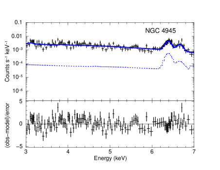
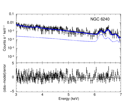
Figure 10: X-ray spectra of NGC 4945 and NGC 6240 taken from the external regions. The upper windows show the observed data (black crosses) and the best-fit models (black solid line), and the lower ones show residuals. The spectra are reproduced by considering the sum of two components: one is from the extracted 2″–4″ region (blue solid line), and the other is from the central point source extended by the PSF (blue dotted line).

5.1.3 Spatially distributed HMXBs for the external Fe-K$\alpha$ emission?

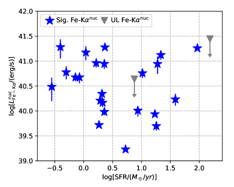
Figure 11: Scatter plots of the SFR and Fe-K$\alpha$ luminosities on the external (left) and nuclear (right) scales. AGNs with significant Fe-K$\alpha$ emission ($L^{\rm ext}_{\rm Fe-K\alpha}/\Delta L^{\rm ext}_{\rm Fe-K\alpha}>1$ or $L^{\rm nuc}_{\rm Fe-K\alpha}/\Delta L^{\rm nuc}_{\rm Fe-K\alpha}>1$) are indicated by blue stars. In contrast, those with upper limits (UL) are shown as gray triangles. No significant correlation is found in either case.

Finally, we discard a scenario in which X-ray binaries (XRBs) strongly contribute to the Fe-K$\alpha$ emission. Among XRBs, high-mass XRBs (HMXBs) contribute more than low-mass XRBs (LMXBs), given the higher detection rate of the Fe-K$\alpha$ emission in HXMBs than in LMXBs (Torrejón et al., 2010). Because a good correlation was found between the total X-ray luminosity of HMXBs in a galaxy and the galaxy-scale star-formation rate (SFR) in a wide SFR range of 0.1–1000 $M_{\odot}$ yr^-1 (Mineo et al., 2012), we examine the relation between the Fe-K$\alpha$ luminosity ($L^{\rm ext}_{\rm Fe-K\alpha}$) and the SFR, as shown in the left panel of Figure 11. The SFRs were taken from Shimizu et al. (2017) and Ichikawa et al. (2019), who derived the SFRs by decomposing spectral energy distributions (SEDs) into AGN and star-formation components. Notably, the far-infrared (FIR) photometry data of the SEDs where star-formation emission is usually significant were obtained at an angular resolution of $\approx$ 6″ of Herschel/PACS at best. However, the FIR source sizes of hard X-ray selected AGN host galaxies at redshifts below 0.05, as with our targets, were found to be at most $\sim$ 3″ at 70 $\mu$m (Mushotzky et al., 2014). Therefore, it is reasonable to compare the SFRs we adopted with the Fe-K$\alpha$ luminosities because they were derived at similar angular scales (2″–4″). As illustrated in Figure 11, the SFR and the Fe-K$\alpha$ luminosity are not correlated ($P$ = $0.19^{+0.10}_{-0.08}$), suggesting that HMXBs do not provide a strong contribution to the observed Fe-K$\alpha$ flux.

As a supplemental check, we examine a relation of the SFR versus the nuclear-scale Fe-K$\alpha$ luminosity (right panel of Figure 11). No significant correlation is found ($P=0.85^{+0.11}_{-0.24}$).

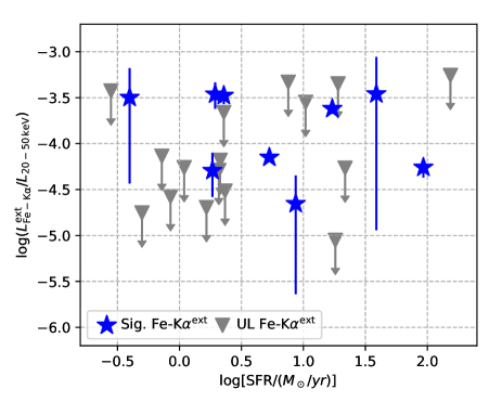
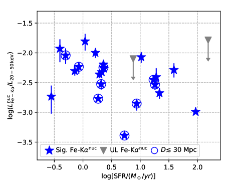
Figure 12: Scatter plots of the SFR and the Fe-K$\alpha$-to-X-ray luminosity ratio on the external (left) and nuclear (right) scales. AGNs with significant Fe-K$\alpha$ emission ($L^{\rm ext}_{\rm Fe-K\alpha}/\Delta L^{\rm ext}_{\rm Fe-K\alpha}>1$ or $L^{\rm nuc}_{\rm Fe-K\alpha}/\Delta L^{\rm nuc}_{\rm Fe-K\alpha}>1$) are indicated by blue stars. In contrast, those with upper limits (UL) are shown by gray triangles. Only in the right panel, open circles are over-plotted for AGNs at distances $\lesssim$ 30 Mpc. No significant correlation is found in either case.

Finally, we assess a correlation between SFR and $L^{\rm ext}_{\rm Fe-K\alpha}/L_{\rm 20-50~{}keV}$, motivated by a recent study by Yan et al. (2021). They suggested a connection between the SFR on a galaxy scale and the EW of the Fe-K$\alpha$ line in a redshift range of 0.5–2. Contrary to this suggestion, no strong link was found between the two physical parameters, as shown in the left panel of Figure 12. However, the SFRs of most of our targets are below 17 $M_{\sun}$ yr^-1, which is the threshold adopted by Yan et al. (2021) to observe a difference in the Fe-K$\alpha$ EW between active and less-active star-forming galaxies. Thus, further studies focusing on rapidly star-forming galaxies are needed to assess the relation between the extended Fe-K$\alpha$ emission and SFR.

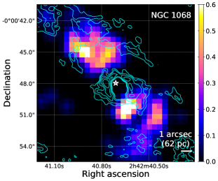
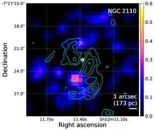
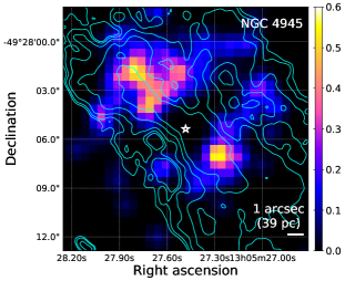
Figure 13: Spatial distributions of CO($J$=2–1) emission (cyan contours) and the ratio of 6–7 and 3–6 keV images from which nuclear point sources are subtracted (color follows right bars) for NGC 1068, NGC 2110, and NGC 4945 from left to right. The panels show the $\approx$ 15″$\times$15″ regions centered at the AGN positions (white stars). North is up and east is left. Cyan contours represent 20$\sigma$, 40$\sigma$, 80$\sigma$, 160$\sigma$, and 230$\sigma$, where 1$\sigma$ = 0.046 Jy km/s per beam for NGC 1068, and 1$\sigma$ = 0.071 Jy km/s per beam for NGC 4945. For NGC 2110, the cyan contours represent 5$\sigma$, 10$\sigma$, 20$\sigma$, and 30$\sigma$, where 1$\sigma$ = 0.060 Jy km/s per beam.

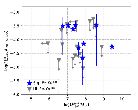
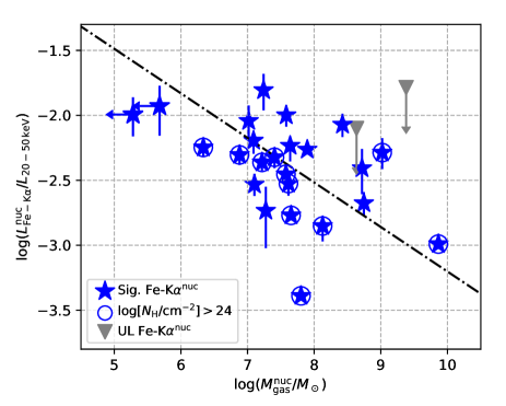
Figure 14: Scatter plots of the molecular gas mass and the Fe-K$\alpha$-to-continuum ratio for the external (left) and nuclear (right) scales. AGNs with significant Fe-K$\alpha$ emission ($L^{\rm ext}_{\rm Fe-K\alpha}/\Delta L^{\rm ext}_{\rm Fe-K\alpha}>1$, or $L^{\rm nuc}_{\rm Fe-K\alpha}/\Delta L^{\rm nuc}_{\rm Fe-K\alpha}>1$) are indicated by blue stars. In contrast, those with upper limits (UL) are shown as gray triangles. In the left figure, NGC 1052 with $\log(M^{\rm ext}_{\rm gas}/M_{\odot})<4$ is located outside. In the right panel, open circles are over-plotted for AGNs whose line-of-sight X-ray absorbing column densities are above $10^{24}$ cm^-2. A trend was found on the nuclear scale but not on the external scale. The dot-dashed line in the right panel is derived using a bootstrap method that incorporates the upper limits.

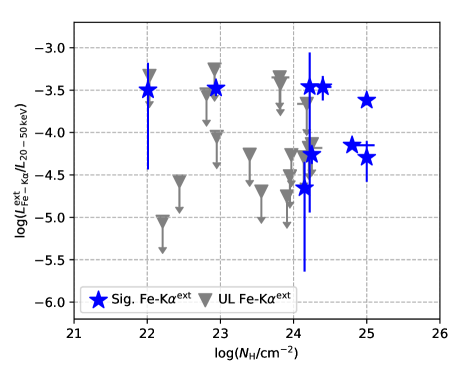
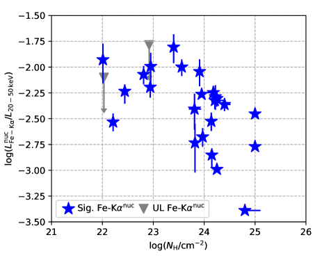
Figure 15: (Left) Scatter plot of the X-ray column density and the ratio between the external Fe-K$\alpha$ and 20–50 keV luminosities. (Right) Same, but for nuclear Fe-K$\alpha$ emission. AGNs with significant Fe-K$\alpha$ emission ($L^{\rm ext}_{\rm Fe-K\alpha}/\Delta L^{\rm ext}_{\rm Fe-K\alpha}>1$ or $L^{\rm nuc}_{\rm Fe-K\alpha}/\Delta L^{\rm nuc}_{\rm Fe-K\alpha}>1$) are indicated by blue stars. In contrast, those with upper limits (UL) are shown as gray triangles.

5.2 Relation of Fe-K$\alpha$ Emitting Sites and Molecular Gas Distributions

We present here that the ALMA CO($J$=2–1) data give us interesting insights into the impact of the AGN X-ray irradiation on the ISM. We take two approaches. First, we compare the distributions of the CO($J$=2–1) and Fe-K$\alpha$ emission, and discuss their spatial relation. As the external Fe-K$\alpha$ emission is not detected for most of the objects, we particularly focus on NGC 1068, NGC 2110, and NGC 4945, for which the external Fe-K$\alpha$ emission is detected at the highest significance levels of $\approx 8\sigma$, $\approx 5\sigma$, and $\approx 10\sigma$, respectively (Table 5). Note that although the external Fe emission of NGC 6240 is significantly detected at $\approx$ 4$\sigma$, we do not discuss this object because we do not correct for the presence of two nuclei in the 6–7 keV-to-3–6 keV image. As detailed later in Section 5.2.3, these highly significant detections are likely due to their higher signal-to-noise ratios. Second, we statistically assess a relation of the CO($J$=2–1) and Fe-K$\alpha$ emission while considering all 26 targets.

5.2.1 Spatial Comparison of the Fe and CO Emission

For NGC 1068, NGC 2110, and NGC 4945, Figure 13 compares the CO($J$=2–1) images and the X-ray ratio (6–7 keV/3–6 keV) images. As discussed in Section 5.1.2, whereas the 6–7 keV spectrum of NGC 4945 includes the Fe-K$\alpha$ and Fe xxv lines, regardless of which is prominent, the ratio can trace photoionized iron atoms. This is also true for NGC 1068. In addition to the Fe-K$\alpha$ line, the external spectrum showed significant emission lines at 6.63$\pm 0.02$ and 6.96$\pm 0.03$ keV in the rest frame (Figure 4). Such high-energy lines have been interpreted as originating from photoionized gas by nuclear X-ray emission (e.g., Bianchi et al., 2001; Ogle et al., 2003). Regarding NGC 2110, only the Fe-K$\alpha$ emission with high EWs of $\sim$ 1.5–1.6 keV, favoring photoionization of iron atoms, was detected. Thus, all X-ray-ratio images likely trace the gas irradiated by the AGN X-ray emission. We discuss the objects separately as follows.

NGC 1068: Fe emission is elongated in the northeast–southwest direction. A similar elongation was observed for the CO($J$=2–1) emission. However, while bright Fe and CO($J$=2–1) emission is observed in the northeast region located $\sim$ 3″ ($\sim$ 180 pc) from the nucleus, they are spatially separated. The extended Fe emission is closer to the nucleus than the CO($J$=2–1) emission. This suggests that the ISM closer to the AGN is preferentially irradiated by the AGN X-ray emission, and the CO($J$=2–1) emission may be suppressed. Whereas there are a few conceivable suppressing mechanisms (e.g., CO and/or H₂ gas destruction or super-thermal), CO molecules may be dissociated into C and O, as recently proposed for a nearby luminous AGN of NGC 7469 by Izumi et al. (2020). However, we do not draw a conclusion regarding the dominant process in this study. For a robust conclusion, additional information is needed. Lastly, in the southwest region, CO($J$=2–1) and Fe distributions appear to be separated, similar to those in the northeast region. These facts suggest that the irradiated gas is seen to be close to the molecular gas, but they are spatially separated, likely owing to the change in the properties of the ISM therein.

NGC 2110: This AGN host galaxy also provides a similar picture to that suggested by NGC 1068. Although the south-bright Fe-K$\alpha$ emission seems to be associated with faint CO($J$=2–1) emission, one can see a clear spatial separation between the brightest CO($J$=2–1) and Fe-K$\alpha$ emission. This is consistent with the fact that AGN X-ray radiation contributes to the change in the physical properties of the ISM. According to Rosario et al. (2019), who studied near- and mid-infrared spectroscopy data of NGC 2110, the north–south region with CO($J$=2–1) deficit and bright Fe-K$\alpha$ emission may be filled by ionized and warm molecular gas. One can also refer to Fabbiano et al. (2019) and Kawamuro et al. (2020) for more details.

NGC 4945: Because this galaxy is an almost edge-on system, it is quite difficult to discuss whether the Fe and CO($J$=2–1) emission is spatially separated or not, such as for NGC 1068 and NGC 2110. However, we remark two important points, suggesting the AGN X-ray irradiation of the ISM. First, the Fe emission is preferentially bright along the galaxy disk in the northeast-to-southwest direction, where CO emission is also bright. Second, fainter Fe emission with 6–7 keV-to-3–6 keV ratios of $\sim 0.15$ is seen over $\sim$ 4″ ($\sim$ 160 pc) in the northwest direction, where the CO($J$=2–1) emission is moderately bright. The distribution appears as a double horn, and this could be due to limb brightening of a hollow, cone shaped outflow oriented close to the plane of sky that was seen and modeled with inclination angle of 75^∘ in Venturi et al. (2017) for optical [N II] emission. Seemingly, the Fe-K$\alpha$ outflow lies closer to the nucleus than [N II], and this may be because the Fe-K$\alpha$ emission is produced by the fluorescent process, which is preferably expected in dense nuclear regions. Thus, given that the outflow is driven by the AGN, it is natural that the AGN X-ray emission irradiates the gas therein.

5.2.2 Relation between Fe-K$\alpha$ and CO($J$=2–1) Emission

To further discuss the possible spatial separation between the cold molecular gas and the Fe-K$\alpha$ emission, we examine the relation between the gas mass ($M^{\rm ext}_{\rm gas}$) and the ratio of the Fe-K$\alpha$ and continuum luminosities ($L^{\rm ext}_{\rm Fe-K\alpha}/L_{\rm 20-50~{}keV}$). As explained in the second paragraph from the last of Section 3, the gas masses were derived from the external CO($J$=2–1) luminosities. The left panel of Figure 14 shows a scatter plot of the two parameters. Here, because the two physical values are derived from the same regions for each object, this discussion is unaffected by differences in object distance. No significant correlation is found with $P\approx 0.7$. While we cannot infer much from the plot, the absence of a positive correlation is consistent with the spatial separation. Thus, by considering the results in Section 5.2.1 (particularly for NGC 1068 and NGC 2110), we suggest that X-ray irradiation may alter the ISM in such a way that it cannot be traced well by CO($J$=2–1) emission.

5.2.3 Relation between Fe-K$\alpha$ and Column Density

Recently, Ma et al. (2020) performed a systematic study of nearby Compton-thick AGNs ($z\sim$ 0.01) to search for extended Fe-K$\alpha$ emission and found it at a relatively high rate (i.e., five out of seven). Following their work, we examine whether there is a relation between the sight-line X-ray absorbing column density and the Fe-line-to-continuum luminosity ratio ($L^{\rm ext}_{\rm Fe-K\alpha}/L_{\rm 20-50~{}keV}$), as shown in the left panel of Figure 15). Although we can find that the detection rate of the extended Fe-K$\alpha$ emission is relatively high for Compton-thick AGNs ($\sim 50$%), it is not so straightforward to conclude the correlation given that some Compton-thick AGNs with $N_{\rm H}\sim 10^{24}$ cm^-2 have low $L^{\rm ext}_{\rm Fe-K\alpha}/L_{\rm 20-50~{}keV}$ ratios, whereas a Compton-thin AGN of NGC 2110 with $\log(N_{\rm H}/{\rm cm}^{-2})\approx 23$ shows a high $L^{\rm ext}_{\rm Fe-K\alpha}/L_{\rm 20-50~{}keV}$ ratio of $\approx 10^{-3.5}$.

We suspect that their spectra with high signal-to-noise ratios and high column densities help the detection, explaining the high detection rate in the Compton-thick AGNs. Simply, a spectrum with a higher signal-to-noise ratio allows the detection of fainter emission. In addition, a higher column density suppresses nuclear emission more, making it easier to detect extended emission. Our suggestion is supported by Figure 16, where the spectral count in the 3–7 keV band is plotted as a function of the column density. In the figure, AGNs with significant Fe-K$\alpha$ detections above 2$\sigma$ have spectra with higher spectral counts and higher column densities. The detection for the Compton-thin AGN NGC 2110 can be explained in the same way. Its spectrum has a high spectral count of $\sim 2500$.

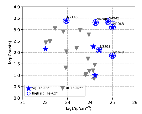
Figure 16: Photon count of the external spectrum in the 3–7 keV band as a function of column density. AGNs with significant Fe-K$\alpha^{\rm ext}$ detections ($L^{\rm ext}_{\rm Fe-K\alpha}/\Delta L^{\rm ext}_{\rm Fe-K\alpha}>1$) are indicated by blue stars. Moreover, open circles and names are overplotted for those with significance levels above 2$\sigma$. In contrast, those with upper limits (UL) are shown as gray triangles. Note that the target names are partly omitted for clarity (e.g., NGC 2110 is presented as N2110).

Figure 17: (Left) Scatter plot of the external-scale molecular gas mass and the absorbing hydrogen column density derived in the X-ray band. NGC 1052 with $\log(M^{\rm ext}_{\rm gas}/M_{\odot})<4$ is located outside. (Right) Same, but for nuclear-scale molecular gas. AGNs with significant CO($J$=2–1) emission ($L^{\rm ext}_{\rm CO}/\Delta L^{\rm ext}_{\rm CO}>1$ or $L^{\rm nuc}_{\rm CO}/\Delta L^{\rm nuc}_{\rm CO}>1$) are indicated by blue stars. In contrast, those with upper limits (UL) are shown as gray triangles.

In addition, we check the hypothesis that AGNs with higher column densities are in gas-rich galaxies (the right panel of Figure 17). With the bootstrap method, no correlation is found ($P=0.55^{+0.14}_{-0.13}$), suggesting that there is no clear connection between the obscuring material and the molecular gas on scales of $\gtrsim 100$ pc. No correlation is confirmed also on the external scales $(P=0.88^{+0.10}_{-0.13}$; the left panel of Figure 17). A connection on smaller scales of $\sim 10$ pc was however suggested by Garcia-Burillo et al. (2021), who found a positive correlation between the line-of-sight column densities derived in the X-ray band and those derived from CO($J$=3–2).

Based on the discussion in Sections 5.1 and 5.2, we argue two points. First, the AGN can form an extended Fe-K$\alpha$ emission by irradiating the surrounding ISM (Section 5.1). Second, the physical and/or chemical properties of the ISM are altered, and such ISM may be missed by CO($J$=2–1) emission or cold molecular gas tracers (Section 5.2). Given that cold gas is the source of star formation, X-ray radiation could potentially function as a negative AGN feedback.

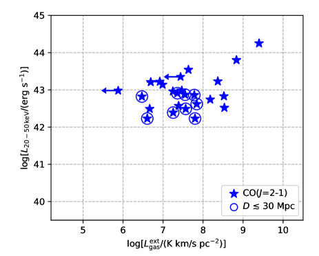
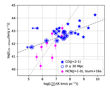
Figure 18: (Left) Scatter plot of the CO($J$=2–1) luminosity in the external region and the X-ray (20–50 keV) luminosity. For the CO($J$=2–1) data of the 10 nearby AGNs at distances $\lesssim$ 30 Mpc, unfilled circles are overplotted. As inferred from the figure, no significant correlation is found. (Right) Dependence of the X-ray (20–50 keV) luminosity on the CO($J$=2–1) luminosity (blue) and HCN($J$=1–0) luminosity (magenta). The CO luminosities are from the nuclear regions, and the HCN ones are retrieved from Izumi et al. (2016a). The unfilled circles are overplotted in the same way as in the left panel. The regression lines derived from the CO($J$=2–1) and HCN($J$=1–0) data (Equations 4 and 5) are indicated by dashed and dotted lines, respectively.

5.3 Nuclear-scale Gas and Mass Accretion onto SMBHs

In this section, we focus on the nuclear regions, where we expect X-ray irradiation to have a stronger effect on the ISM.

5.3.1 Molecular Gas Mass and Accretion Rate

To reveal the potential effect of X-ray radiation on the ISM, we first investigate a link between the mass of the surrounding cold molecular gas and the mass accretion rate. Similar studies have already been conducted. For example, Yamada (1994) presented a significant correlation between the X-ray (0.5–4.5 keV) and CO($J$=1–0) luminosities for a nearby sample of 13 Seyfert 1 galaxies and 5 quasars, supporting the link. The correlation was further assessed using larger samples. Monje et al. (2011) found a significant correlation between the CO($J$=2–1) and X-ray (0.3–8 keV) luminosity for 45 nearby Seyfert galaxies including type-1 and type-2 objects ($P$ = $2\times 10^{-7}$) (see also Shangguan et al., 2020). However, a more recent study by Koss et al. (2021), who used CO($J$=2–1) and X-ray-based bolometric luminosities, did not find a significant correlation for an ultrahard X-ray ($>$ 10 keV) sample consisting of $\approx$ 200 AGNs. In this context, our study can give new insights by exploiting the much higher resolutions of ALMA than those of single-dish telescopes used in previous studies (i.e., NRAO 12-m, CSO, JCMT, and APEX). Specifically, we investigate the correlation by considering the physical scale of cold molecular gas or by separating the nuclear and external regions.

First, we examine their correlation in the external scale by using the 20–50 keV luminosity ($L_{\rm 20-50~{}keV}$) and the CO($J$=2–1) luminosity ($L^{\rm ext}_{\rm CO({\it J}=2-1)}$) as proxies of the accretion rate and the gas mass, respectively. The measured values are listed in Tables 1 and 4. A scatter plot of $L_{\rm 20-50~{}keV}$ and $L^{\rm ext}_{\rm CO({\it J}=2-1)}$ is shown in the left panel of Figure 18. Adopting the same bootstrap analysis as used previously in Section 5.1.1, we obtain

$$\log (L_{\rm 20-50~{}keV}/{\rm erg~{}s}^{-1})=39.5^{+0.3}_{-0.2}$$ (1)

$$+0.46^{+0.02}_{-0.04}\log(L^{\rm ext}_{\rm CO({\it J}=2-1)}/{\rm K~{}km~{}s^{-1}~{}pc}^{-2})$$

with $P=0.25^{+0.07}_{-0.04}$ and $\rho_{\rm s}=0.23\pm 0.03$. No significant correlation is found. Furthermore, to reduce the effect caused by differences in object distance as much as possible, we apply the bootstrap analysis to only 10 nearby AGNs within $D\lesssim 30$ Mpc, where the inner radii of the external regions (2″) span a range of $\approx$ 80–300 pc with a median of $\approx$ 200 pc. The derived regression line is

$$\log (L_{\rm 20-50~{}keV}/{\rm erg~{}s}^{-1})=40.4^{+0.3}_{-0.2}$$ (2)

$$+0.30^{+0.02}_{-0.03}\log(L^{\rm ext}_{\rm CO({\it J}=2-1)}/{\rm K~{}km~{}s^{-1}~{}pc}^{-2})$$

with $P=0.31^{+0.05}_{-0.06}$ and $\rho_{\rm s}=0.38^{+0.10}_{-0.08}$. We cannot find significant correlation. These insignificant correlations can be inferred from the left panel of Figure 18, where a flat distribution of data points is observed in the range $L^{\rm ext}_{\rm CO({\it J}=2-1)}\approx 10^{6-8.5}$ K km s^-1 pc^-2. Thus, there seems to be no strong link between the accretion rate and cool, molecular gas on a scale larger than $\sim$ 200 pc.

We then focus on the nuclear scale, as shown in the right panel of Figure 18. In the same way, we derive a regression line for the entire sample as

$$\log (L_{\rm 20-50~{}keV}/{\rm erg~{}s}^{-1})=39.3^{+0.3}_{-0.2}$$ (3)

$$+0.47^{+0.02}_{-0.03}\log(L^{\rm nuc}_{\rm CO({\it J}=2-1)}/{\rm K~{}km~{}s^{-1}~{}pc}^{-2}).$$

The $p$-value and the Spearman rank coefficient are $P=0.048^{+0.009}_{-0.012}$ and $\rho_{\rm s}=0.39\pm 0.02$, respectively. This result suggests a positive trend. For the nearby 10 AGNs, we obtain

$$\log (L_{\rm 20-50~{}keV}/{\rm erg~{}s}^{-1})=39.6^{+0.5}_{-0.2}$$ (4)

$$+0.41^{+0.03}_{-0.06}\log(L^{\rm nuc}_{\rm CO({\it J}=2-1)}/{\rm K~{}km~{}s^{-1}~{}pc}^{-2})$$

with $P=0.047^{+0.034}_{-0.032}$ and $\rho_{\rm s}=0.64^{+0.10}_{-0.06}$. The trend is then found to still remain, even for the limited sample for which the median of the outer radii of the nuclear regions (2″) is $\approx$ 200 pc. These results suggest that the molecular gas on a scale smaller than $\sim$ 200 pc is well linked to mass accretion onto the central SMBH.

To extend the discussion, we present a correlation analysis between the HCN($J$=1–0) and the X-ray luminosities. The HCN($J$=1–0) line traces much denser gas than CO($J$=2–1), because its critical density of $\sim 10^{6}$ cm^-3 is much higher than that of CO($J$=2–1) ($\sim 10^{3}$ cm^-3 ). Izumi et al. (2016a) compiled HCN data obtained with interferometers (i.e., Plateau de Bure Interferometer, Nobeyama Millimeter Array, and ALMA) for 10 nearby AGNs ($D\sim$ 20 Mpc, except for one at 70 Mpc). The median of their resolutions or the beam sizes was $\approx$ 220 pc. They found a positive trend with the 2–10 keV luminosity ($P=0.058$). To compare the HCN($J$=1–0) result with our CO($J$=2–1) result as consistently as possible, we searched the literature for the 20–50 keV luminosities of the 10 AGNs with the HCN luminosities. We found X-ray luminosities for all but NGC 6951. By performing the bootstrap analysis on the updated HCN sample, a regression line is obtained as

$$\log (L_{\rm 20-50~{}keV}/{\rm erg~{}s}^{-1})=31.9\pm 1.1$$ (5)

$$+1.5\pm 0.2\log(L_{\rm HCN({\it J}=1-0)}/{\rm K~{}km~{}s^{-1}~{}pc}^{-2})$$

with $P=0.036^{+0.063}_{-0.026}$ and $\rho_{\rm s}=0.7^{+0.1}_{-0.2}$, suggesting a positive trend. Here, the uncertainties in the HCN($J$=1–0) luminosities are taken from Izumi et al. (2016a). Those in the 20–50 keV luminosities are set to 0.3 dex uniformly by following Izumi et al. (2016a). While some luminosities were derived based on Swift/BAT average spectra (Ricci et al., 2017a), others were estimated by a single epoch hard X-ray observation (i.e., NGC 1097, NGC 4579, and NGC 2273; Nemmen et al., 2006; Masini et al., 2016; Younes et al., 2019). Therefore, to account for the short-time flux variability, we adopt the uncertainty of 0.3 dex. For simplicity, we consider the same uncertainty even if a luminosity was derived from a long-term averaged BAT spectrum.

An intriguing fact can be suggested from the possibility that the ratio of CO-to-HCN luminosities increases with $L_{\rm 20-50\,keV}$. However, we note that our argument relies on the extrapolation of the regression lines due to a small overlap of the CO and HCN samples in the X-ray luminosity range, which suggests that the ratio of the CO($J$=2–1) and HCN($J$=1–0) luminosities increases with X-ray luminosity. Quantitatively, for an increase in X-ray luminosity by an order of magnitude, the ratio changes by a factor of $\approx$ 30–60.

Whether the above result is inconsistent with the HCN-enhancement in AGN host galaxies discussed in previous studies (e.g., Kohno, 2005; Krips et al., 2008; Imanishi et al., 2009; Izumi et al., 2016b) may be debated. We argue that there is no clear discrepancy with our result. For example, Kohno (2005) compiled the data of CO($J$=1–0) and HCN($J$=1–0) on scales of a few hundred parsecs using the Nobeyama Millimeter Array. He then proposed that pure AGNs showed higher HCN($J$=1–0)-to-CO($J$=1–0) ratios ($\gtrsim 0.2$) than composite objects (i.e., an AGN co-exists with nuclear starburst). Here, by paying attention to the X-ray luminosities of his targeted AGNs, we notice an interesting point. Three of the four pure AGNs are X-ray faint as $L_{\rm 2-10\,keV}=10^{40-41}$ erg s^-1, with the remaining object of NGC 1068 having $L_{\rm 2-10\,keV}\approx 10^{43}$ erg s^-1. On the contrary, all composite galaxies, except NGC 6764 with $L_{\rm 2-10\,keV}=10^{39.9}$ erg s^-1, are X-ray luminous with $L_{\rm 2-10\,keV}=10^{41-43}$ erg s^-1. Thus, a decreasing trend of the HCN($J$=1–0)/CO($J$=1–0) ratio with X-ray luminosity is observed, which is consistent with our results. Although we focus on the X-ray luminosity to discuss the HCN enhancement, there are other energetic phenomena to be considered, such as the AGN jet and the outflow. Thus, a more detailed discussion of individual objects is encouraged in future papers.

5.3.2 Explanation for Trends of X-ray and Molecular Line Emission Luminosities

To explain the increasing CO($J$=2–1)-to-HCN($J$=1–0) ratio with X-ray luminosity, we suggest that the decrease in gas density must be taken into consideration in addition to other possible causes, such as a change in the abundance ratio between HCN and CO molecules and the effective heating of CO molecules. For the discussion, we refer to an extensive numerical study of Meijerink et al. (2007). While considering the thermal and chemical balances of gas, they calculated the intensities of emission lines from molecular and atomic gases exposed to FUV and X-ray radiation over a large range of gas densities ($\sim 10^{2-6}$ cm^-3). Here, we focus particularly on the results in the range $10^{5-6}$ cm^-3, which covers a critical density of $\sim 10^{6}$ cm^-3 for HCN($J$=1–0) and also those of observationally suggested HCN($J$=1–0) emitting gas ($\sim 10^{5}$ cm^-3; e.g., Krumholz & Tan 2007). As shown in their Figure 12, they found that for the density range, the ratio of CO($J$=1–0)/HCN($J$=1–0) changes insignificantly over a wide range of incident X-ray flux of 1–100 erg cm^-2 s^-1. The result can be applied to our AGNs, as their 1–100 keV fluxes are $\approx$ 2–20 erg cm^-2 s^-1 at 1″ from the center, or $\sim$ 200 pc as the median value. Here, we assume that the X-ray photons from an AGN are not heavily absorbed until they reach a gas cloud. Under such circumstances, Meijerink et al. (2007) also suggested that the CO($J$=2–1)/CO($J$=1–0) ratio is almost unchanged with an increase in X-ray luminosity by one order of magnitude (their Figure 4). Thus, combined with almost no change in the CO($J$=1–0)/HCN($J$=1–0) ratio with X-ray luminosity, X-ray heating is insufficient to explain the observed rapid increase in CO($J$=2–1) luminosity. Hence, a decrease in the gas density remains the explanation for the rapid increase in the CO($J$=2–1)/HCN($J$=1–0) ratio. Indeed, Meijerink et al. (2007) predicted that the CO($J$=1–0)/HCN($J$=1–0) ratio could be rapidly increased (their Figure 12) with decreasing gas density because with decreasing density, HCN($J$=1–0) with a high critical density becomes weaker. Quantitatively, to explain the factor of $\approx$ 30–-60 decrease in HCN($J$=1–0)/CO($J$=2–1), the gas density must decrease by a factor of $\sim$ 10. In summary, whereas the X-ray heating may have an impact on the line ratio, a decrease in the molecular gas density must be considered.

5.3.3 Physical Mechanism to Reduce Gas Density around the AGN

Why can the gas density decrease around an X-ray luminous AGN? This may be due to the evaporation of gas clouds by harsh X-ray radiation.

As a supportive study for the evaporation picture, we refer to Hocuk & Spaans (2011), who performed numerical simulations to investigate dynamical evolution of gas clouds located 10 pc from central mass-accreting SMBHs. The gas clouds were exposed to AGN X-ray radiation, and UV emission and cosmic rays originating from star-formation activity were also considered as the other possible mechanisms affecting the gas clouds (see also Hocuk & Spaans, 2010). The incident X-ray fluxes into gas clouds range over 0–160 erg cm^-2 s^-1, and encompass the expected fluxes for our AGNs, as mentioned previously (i.e., 2–20 erg cm^-2 s^-1). In contrast, some of our SMBH masses are larger by $\sim$ one order of magnitude than the range considered in their work (10${}^{6-8}M_{\odot}$). Specifically, among 15 AGNs whose SMBH masses were estimated using stellar dispersions in Koss et al. (2017), nine have masses larger than $10^{8}~{}M_{\odot}$ and the others have masses within the range of $10^{7-8}~{}M_{\odot}$. However, we consider molecular clouds located further away than 10 pc (a fixed distance used by the authors in their modeling), therefore we may simply refer to models where gravity from the BH is weak (i.e., models with BH mass of $10^{6}M_{\odot}$).

An intriguing result of Hocuk & Spaans (2011) is that stronger X-ray emission evaporates a larger portion of the gas cloud. In harsh conditions, even a dense gas ($>10^{5}$ cm^-3) can be affected despite its strong self-shielding. Eventually, the mass of gas with high densities ($>10^{5}$ cm^-3) decreases (e.g., see the simulation results with M04, M10, M16, and M22, in their Figure 7). Given that the resultant gas whose density is globally reduced would not be favored to excite HCN($J$=1–0) but would still manage to excite CO($J$=2–1), the prediction is qualitatively consistent with our finding (i.e., the CO($J$=2–1)-to-HCN($J$=1–0) ratio increases with X-ray luminosity).

The above evaporation, or outflow, picture is supported by a negative trend between the ratio of $\log(L^{\rm nuc}_{\rm Fe-K\alpha}/L_{\rm 20-50~{}keV}$) and the molecular gas mass, as shown in the right panel of Figure 14. The bootstrap analysis suggests their negative trend with $P=0.05^{+0.11}_{-0.04}$ and $\rho_{\rm s}=-0.39\pm 0.11$. A regression line is derived as

$$\log (L^{\rm nuc}_{\rm Fe-K\alpha}/L_{\rm 20-50~{}keV})$$ (6)

$$=0.23^{+0.28}_{-0.22}-0.34^{+0.03}_{-0.04}\log(M^{\rm nuc}_{\rm gas}/M_{\odot}).$$

The $L^{\rm nuc}_{\rm Fe-K\alpha}/L_{\rm 20-50~{}keV}$ ratio can be used as a proxy for the solid angle of gas irradiated by the AGN X-ray emission. Also, given the positive trend of $L_{\rm 20-50~{}keV}$ and $M^{\rm nuc}_{\rm gas}$, as inferred from the right panel of Figure 18, the equation can suggest that more luminous AGNs are less covered by dense gas that can be traced by Fe-K$\alpha$ emission. This is qualitatively consistent with a radiation-driven outflowing model (e.g., Fabian et al., 2009; Ricci et al., 2017b; Ogawa et al., 2021), where more surrounding material is blown away by stronger AGN emission.

Furthermore, the radiation-driven model can be inferred from the right panel of Figure 15, showing a scatter plot of $L^{\rm nuc}_{\rm Fe-K\alpha}/L_{\rm 20-50~{}keV}$, or the covering factor, versus $N_{\rm H}$. Their rank coefficient is negative as $\rho_{\rm S}=-0.36^{+0.09}_{-0.10}$, although the significance is low with $P=0.07^{+0.11}_{-0.05}$. This negative $\rho_{\rm S}$ value is indeed consistent with a model prediction of Fabian et al. (2009) (e.g., see their Figure 1) that AGNs with higher Eddington ratios tend to have higher absorbing column densities and lower covering factors (Ricci et al., 2017a), thus inferring a negative trend of covering factor and column density.

One might think that the decrease of $L^{\rm nuc}_{\rm Fe-K\alpha}/L_{\rm 20-50~{}keV}$ with $N_{\rm H}$ suggests the absorption of Fe-K$\alpha$ emission, especially in Compton-thick AGNs with $N_{\rm H}>10^{24}$ cm^-2 (e.g., Ricci et al., 2014), and wonder whether the absorption affects the discussion on the negative trend between $L^{\rm nuc}_{\rm Fe-K\alpha}/L_{\rm 20-50~{}keV}$ and $M^{\rm nuc}_{\rm gas}$, or the outflow picture. To see the possibility of the absorption effect, regression lines between $L^{\rm nuc}_{\rm Fe-K\alpha}/L_{\rm 20-50~{}keV}$ and $M^{\rm nuc}_{\rm gas}$ are constrained for Compton-thin and Compton-thick AGN samples, and are found to have normalizations of $0.30^{+0.05}_{-0.06}$ and $0.045^{+0.022}_{-0.021}$, respectively. Here, the slopes are fixed at that of Equation (6) to focus on the normalization. The lower normalization for the Compton-thick AGNs is in fact consistent with their Fe-K$\alpha$ emission being absorbed. However, even if there is the effect of the absorption, that does not affect our argument. To reduce the influence of the absorption, we derive regression lines for the Compton-thin and Compton-thick samples by leaving slope and normalization as free parameters. For these samples, we obtain slopes of $-0.26^{+0.05}_{-0.07}$ and $-0.38\pm 0.02$, respectively, and both negative values are consistent with the outflow picture.

In Figure 19, we schematically illustrate the association between the central X-ray radiation and the surrounding molecular gas based on the above discussion. The figure shows that the mass accretion rate increases with the surrounding gas mass, and the resultant stronger AGN X-ray radiation evaporates a larger fraction of dense gas, yielding tenuous gas, and blows it out, reducing the gas covering fraction.

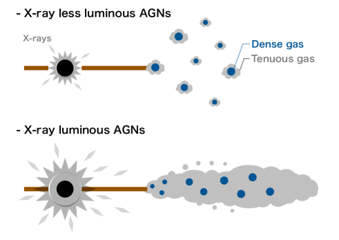
Figure 19: Schematic of the nuclear region. This presents three key points. (i) X-ray emission is enhanced with increasing the molecular gas mass. (ii) A larger fraction of surrounding gas is evaporated by stronger X-ray radiation, which reduces the global (averaged) gas density. (iii) Stronger X-ray radiation also induces outflow, leading to a decreased gas covering factor.

A natural prediction from this picture is that the AGN X-ray irradiation affects the surrounding star formation because dense gas is the site for this process. As discussed in the right panel of Figure 18, the dense gas fraction would decrease with the X-ray luminosity. Given that the dense gas fraction is a key parameter determining the star-formation efficiency (e.g., Gao & Solomon, 2004; Bigiel et al., 2015), the AGN may have the potential to reduce the star-formation efficiency. This was also suggested from the hydrodynamical simulations of Hocuk & Spaans (2011). Consequently, this theoretical work further suggests that even the initial mass function of stars may be altered.

Motivated by Figure 4 of Gao & Solomon (2004), showing that a dramatic increase of HCN($J$=1–0)-to-CO($J$=1–0) luminosity ratio for luminous and ultra-luminous infrared galaxies (i.e., very actively star-forming galaxies), we assess the correlation between $L^{\rm nuc}_{\rm Fe-K\alpha}/L_{\rm 20-50~{}keV}$ and SFR (the right panel of Figure 12). A negative trend is favored from $\rho_{\rm S}=-0.32^{+0.07}_{-0.11}$, while no significant correlation is found ($P$ = $0.12^{+0.12}_{-0.09}$). We note that for a sample of the nearest AGNs with $D\lesssim$ 30 Mpc, $\rho_{\rm S}=-0.47^{+0.14}_{-0.07}$ and $P$ = $0.21^{+0.08}_{-0.07}$. Thus, with our data, we cannot explicitly suggest that the star formation is being suppressed by X-ray irradiation. However, given that the SFRs were measured at larger apertures than 2″  of the nuclear regions, it would be too early to conclude the absence of the effect.

In summary, as our second response to the main question, we suggest that the AGN hard X-ray radiation has the potential to suppress the surrounding star formation by evaporating as well as blowing out the surrounding gas. Thus, this type of negative AGN feedback may be triggered by AGN hard X-ray emission.

6 Summary

Our main goal in this study is to understand what impact the hard X-ray irradiation has on the ISM and star formation. For this purpose, we have performed a systematic analysis of ALMA and Chandra data taken for 26 nearby ($z<0.05$ or $D\lesssim$ 200 Mpc) AGNs, selected from the 70-month Swift/BAT ultrahard X-ray catalog (Baumgartner et al., 2013). By exploiting their high-resolution data, we defined the nuclear region with a central radius of 2″ and the external annular region of 2″–4″. The 2″ scale corresponds to $\sim$ 100–600 pc for the majority of our AGNs (19 out of 26 AGNs).

First, by focusing on the external regions, we suggest that the AGN can form extended hard X-ray emission by irradiating the surrounding ISM, and it is difficult to trace the X-ray-irradiated gas by the CO($J$=2–1) line (Section 5.1; Section 5.2). Thus, AGN X-ray irradiation has the potential to alter the physical and chemical properties of ISM. This suggestion is based on the following findings.

• We find that the $L^{\rm ext}_{\rm Fe-K\alpha}/L_{\rm 20-50~{}keV}$ ratio, a proxy for the solid angle of gas irradiated by AGN X-ray emission, does not correlate with the scattering fraction ($f_{\rm scat}$), disfavoring Thomson scattering as the general mechanism that forms extended Fe-K$\alpha$ emission (Figure 9 and Section 5.1.1).

• We find that, particularly for some AGNs with bright Fe lines, the properties of the Fe lines (e.g., high EW and highly ionized Fe lines) suggest photoionized gas as their origin (Section 5.1.2).

• No correlation is found between the external Fe-K$\alpha$ luminosity ($L^{\rm ext}_{\rm Fe-K\alpha}$) and the galaxy-scale SFR. This supports the idea that HMXBs, one of the most plausible classes of stellar objects that emit Fe-K$\alpha$ photons, do not strongly contribute to the extended Fe-K$\alpha$ emission (Section 5.1.3 and Figure 11).

• By comparing the CO($J$=2–1) and X-ray ratio (6–7 keV/3–6 keV) images in the two AGNs with the well-detected Fe-K$\alpha$ emission (NGC 1068 and NGC 2110), we find that regions with bright Fe emission appear to be separated from those with CO($J$=2–1) emission. For the other galaxy of NGC 4945 with significant Fe-K$\alpha$ emission ($\approx 10\sigma$), it is difficult to discuss the spatial relation between the Fe and CO($J$=2–1) emission because of the edge-on view. However, the brighter Fe emission in its galaxy disk and fainter one in an outflow region would suggest that X-ray irradiation occurs (Section 5.2.1 and Figure 13).

• We find no significant correlation between the the extended Fe-K$\alpha$ emission ($L^{\rm ext}_{\rm Fe-K\alpha}/L_{\rm 20-50~{}keV}$) and the mass of the cold molecular gas ($M^{\rm ext}_{\rm gas}$). This is consistent with the spatial separation (Section 5.2.2 and Figure 14).

Furthermore, we have suggested that the AGN hard X-ray radiation has the potential to suppress the surrounding star formation by evaporating and blowing out the surrounding gas. Thus, negative AGN feedback may be triggered by AGN hard X-ray emission. The results on which our suggestion is based are as follows:

• We find a positive trend between the 20–50 keV luminosity ($L_{\rm 20-50~{}keV}$) and the nuclear CO($J$=2–1) luminosity ($L^{\rm nuc}_{\rm CO}$). Furthermore, we confirm a positive trend between the 20–50 keV luminosity ($L_{\rm 20-50~{}keV}$) and the nuclear HCN($J$=1–0) luminosity ($L^{\rm nuc}_{\rm HCN}$) as well (Section 5.3.1 and Figure 18).

• Based on the above obtained trends, we further find that the ratio of CO($J$=2–1)-to-HCN($J$=1–0) luminosities increases with the 20–50 keV luminosity, suggesting a decrease in the dense gas fraction with X-ray luminosity (Section 5.3.2).

• A negative trend is found between $L^{\rm nuc}_{\rm Fe-K\alpha}/L_{\rm 20-50~{}keV}$ and $M^{\rm nuc}_{\rm gas}$. Given the positive trend between $L_{\rm 20-50~{}keV}$ and $M^{\rm nuc}_{\rm gas}$ (Figure 18), this is consistent with a radiation-driven AGN outflow model (e.g., Fabian et al., 2009; Ricci et al., 2017b). This is supportive evidence for the evaporation of gas in the nuclear region (Section 5.3.3).

Future studies using other molecular and atomic emission lines will help to constrain the physical parameters, such as density, and kinetic temperature, and the chemical abundance. These are valuable for a better understanding of the relation between the AGN and its circumnuclear material. In addition, our sample is limited to nearby AGNs ($\lesssim$ 200 Mpc). However, future high-resolution X-ray telescopes (e.g., AXIS and Lynx; The Lynx Team, 2018; Mushotzky et al., 2019) will improve this situation and provide opportunities to study distant and much more luminous AGNs. They are likely to be interesting targets because they are expected to affect the surrounding ISM and star formation on larger scales ($\gg$ 100 pc). Finally, much sharper images anticipated from a super-resolution of MIXIM down to $\lesssim 0\arcsec.01$–0.″1 will provide valuable opportunities to resolve nuclear structures of nearby AGNs at $<$ 10 pc (Hayashida et al., 2018; Asakura et al., 2020).

Appendix A Negligible Impact of Absorption on Nuclear CO($J$=2–1) Luminosity

Here, we show that CO($J$=2–1) absorption inferred in some objects (e.g., see Figure F of NGC 3081, NGC 4945, NGC 5506, and NGC 5728) would not have a strong impact on the emission flux estimate. This suggestion is based on a detailed analysis of the CO spectrum of NGC 4945. This object is selected owing to its proximity ($\sim$ 8 Mpc); the nuclear spectrum is expected to be easily affected by nuclear absorption lines. The spectrum is extracted from the AGN position with a beam of 0″.34$\times$0″.31 (Figure 20). The central spectrum is subject to absorption most severely and is adopted to see the strongest impact. In the spectrum of Figure 20, two absorption lines appear, and accordingly, we fit three Gaussian functions. One is used to reproduce the emission, and the other two functions are used to consider the absorption lines. Such an analysis was performed for nearby AGNs with absorption lines around the nuclei (e.g., Rose et al., 2019). Figure 20 shows that the adopted model captures the overall shape of the observed spectrum. With this model, we find that the flux density of the absorption-corrected emission line is $\approx$ 66 Jy/beam km/s, and given the observed flux density of $\approx$ 49 Jy/beam km/s, we may underestimate the nuclear CO luminosity of NGC 4945 by $\approx$ 25%. Furthermore, as a less model-independent method, we fit a single Gaussian function to the side velocity bands of 100–440 km/s and 700–1100 km/s, where the absorption lines are not significant. Thus, the fitted function is expected to trace the intrinsic shape of the emission, and we derive its flux to be $\sim$ 70 Jy/beam, which is almost the same as that derived by using the three functions. In both estimates, the degree of underestimate is small on a logarithmic scale, as it corresponds to $\sim$ 0.1 dex. A smaller effect is expected in the outer regions. Thus, there would not be a strong impact on the flux estimates and, consequently, the overall discussion.

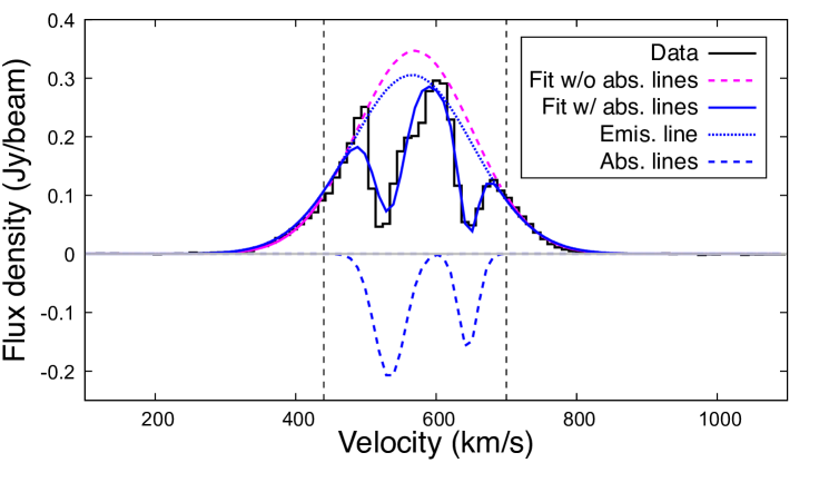
Figure 20: CO($J$=2–1) spectrum (black solid line) extracted from the AGN position of NGC 4945 with a beam of 0″.34$\times$0″.31. The blue solid line indicates the best-fit model that considers one emission line (blue dotted line) and two absorption lines (blue dashed lines). The magenta line indicates the emission model fitted to the velocity ranges of 100–440 km/s and 700–1100 km/s, where absorption is negligible. The two black vertical dashed lines indicate 440 km/s and 700 km/s.

Appendix B Nuclear and external X-ray spectra

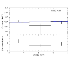
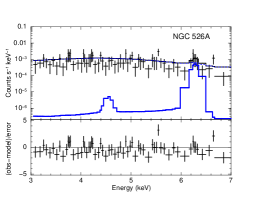
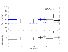
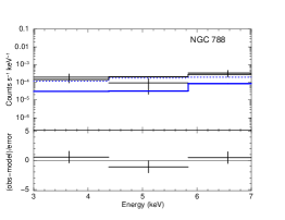
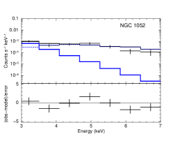
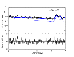
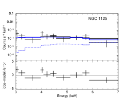
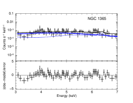
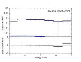
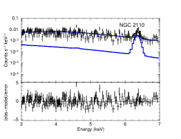
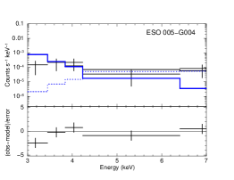
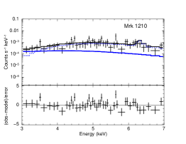
Figure 21: X-ray spectra from the nuclear 2″ regions (first and third columns), and those taken from the external annulus regions with radii of 2″–4″ (2nd and 4th columns). In each nuclear spectral figure, the upper window shows observed data (crosses) and a best-fit model (solid line), and the lower one shows the residuals. For each external spectrum, an in-situ emission and a contaminating emission from a nuclear source (Sections 5.2.2 and 5.3.1) are additionally shown by the blue solid and dotted lines, respectively.

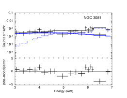
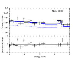
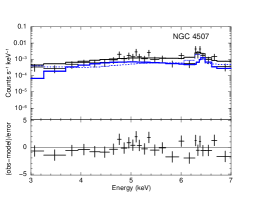
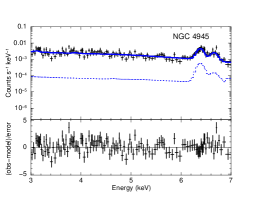
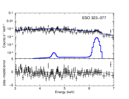
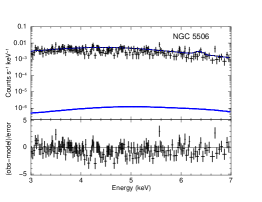
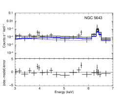
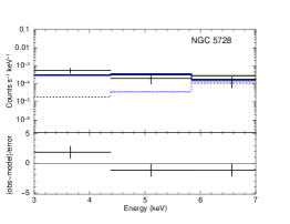
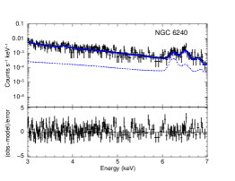
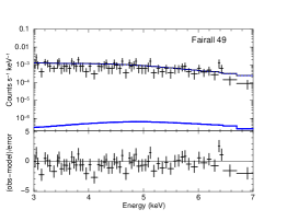
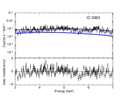
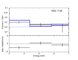
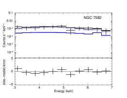
Figure 21: Continued.

Appendix C Radial distributions of X-ray emission

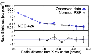
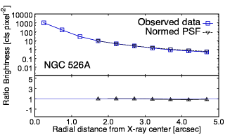
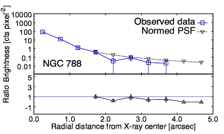
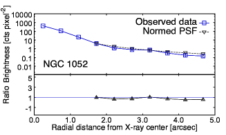
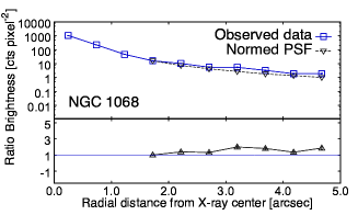
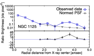
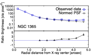
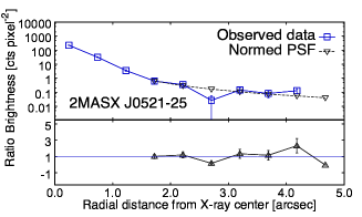
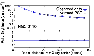
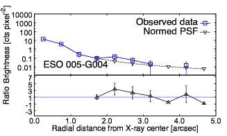
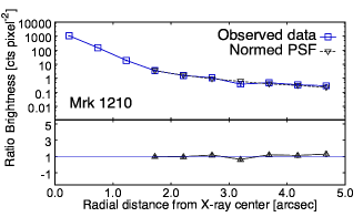
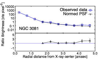
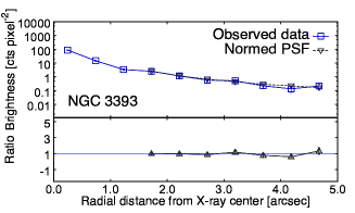
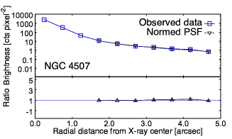
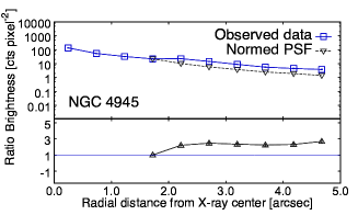
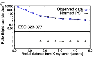
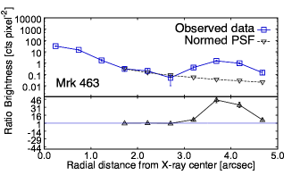
Figure 22: Comparisons of observed (blue) and modeled (black) radial profiles in the 3–6 keV band. The lower windows show the ratios between the observed and modeled radial profiles.

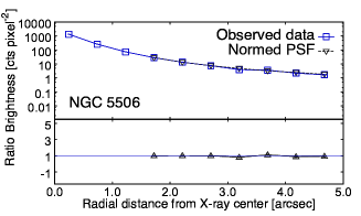
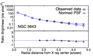
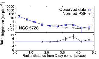
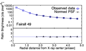
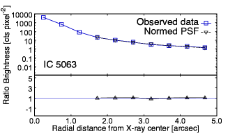
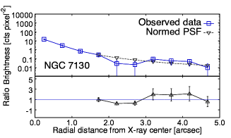
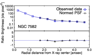
Figure 22: Continued.

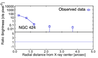
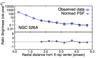
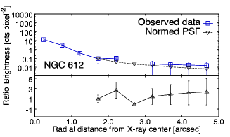
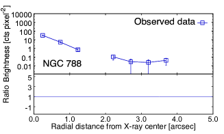
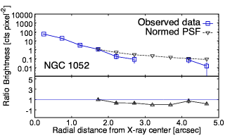
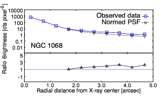
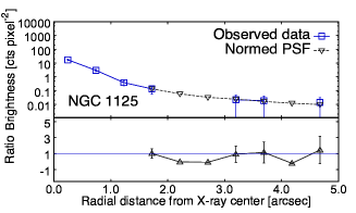
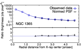
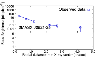
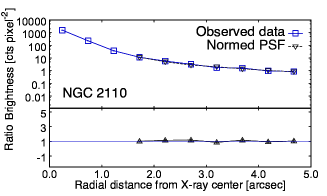
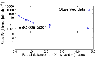
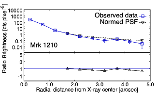
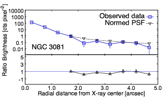
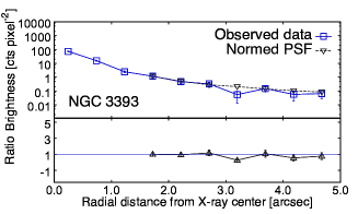
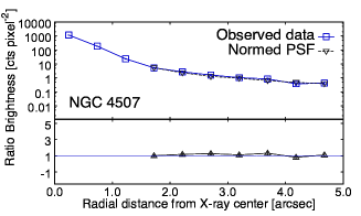
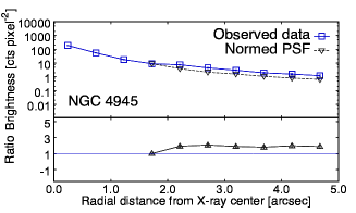
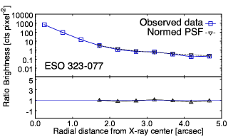
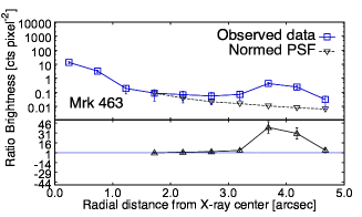
Figure 23: Same as Figure 22, but for the 6–7 keV band. Only observed data are shown for the targets for which we cannot model a profile by normalizing the PSF model at 3.5 pixels, or the 4th pixel, from the center.

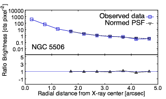
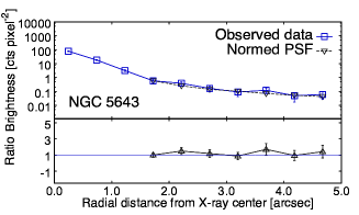
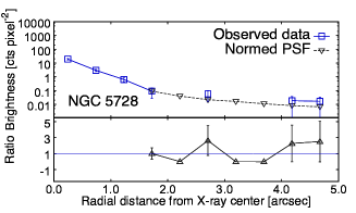
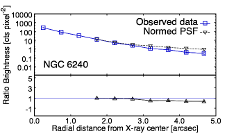
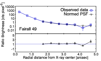
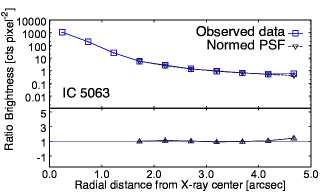
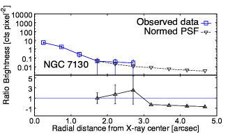
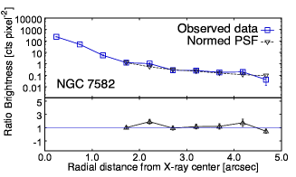
Figure 23: Continued.

Appendix D X-ray images at 3–6 keV and 6–7 keV and their ratios

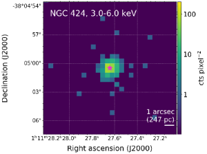
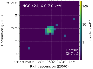
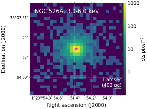
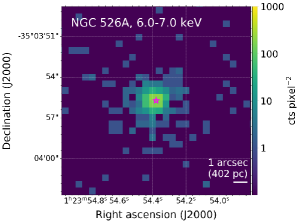
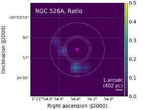
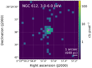
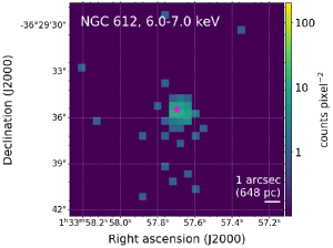
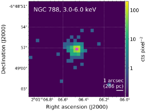
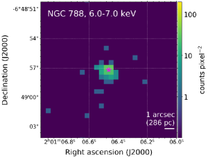
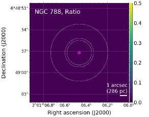
Figure 24: From left to right columns, 3.0–6.0 keV and 6.0–7.0 keV images in units of counts pix^-2 and the ratios of the 6.0–7.0 keV and 3.0–6.0 keV images from which nuclear components are subtracted. North is up and east is left.

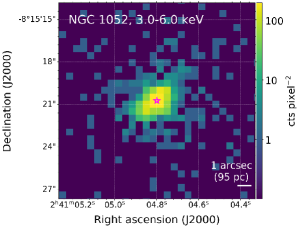
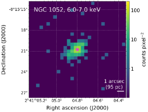
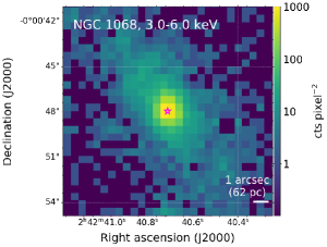
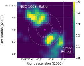
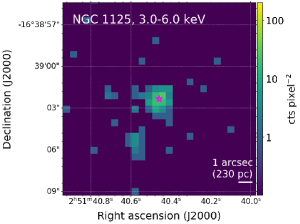
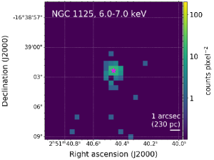
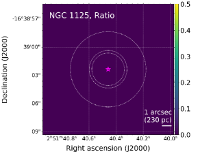
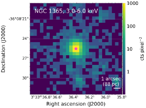
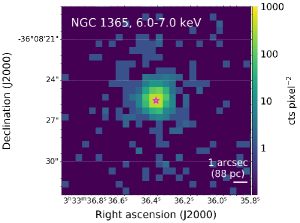
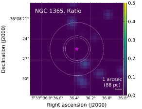
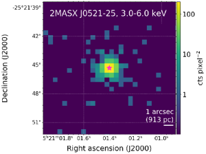
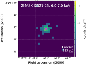
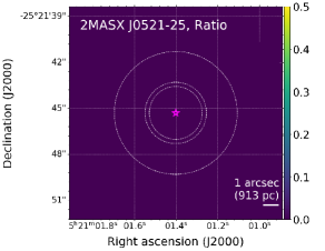
Figure 24: Continued.

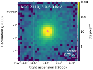
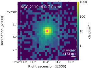
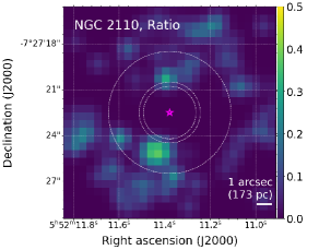
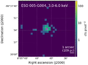
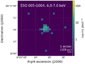
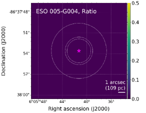
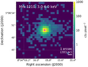
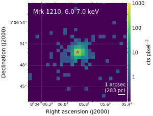
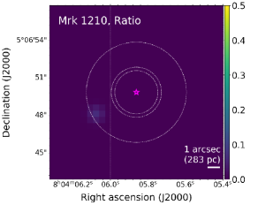
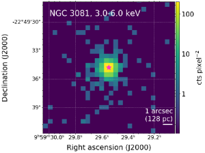
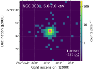
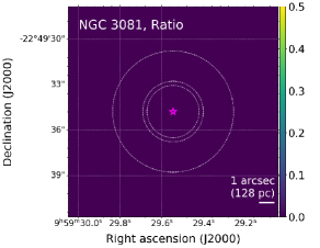
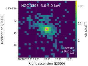
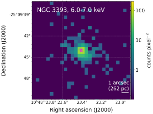
Figure 24: Continued.

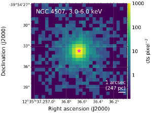
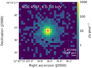
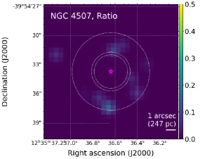
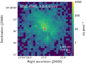
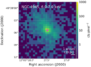
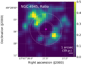
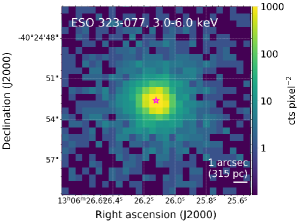
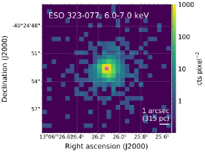
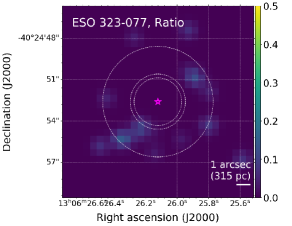
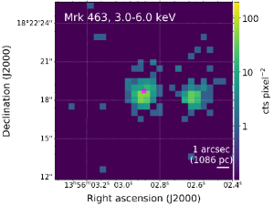
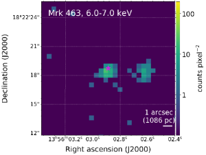
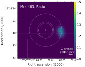
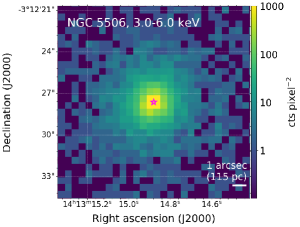
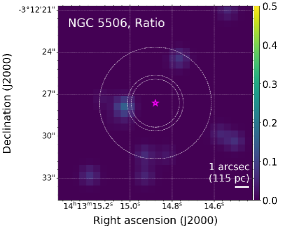
Figure 24: Continued.

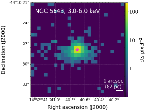
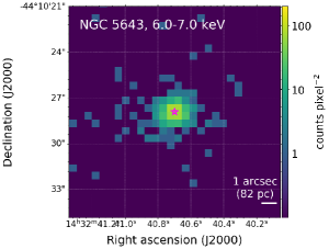
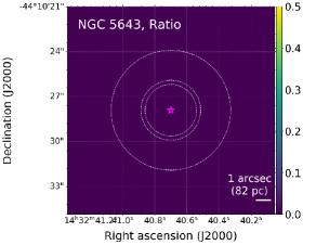
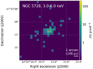
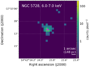
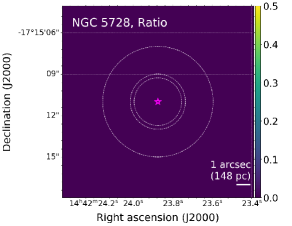
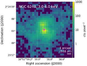
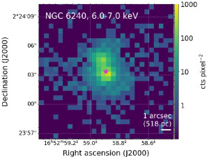
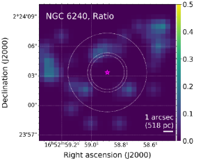
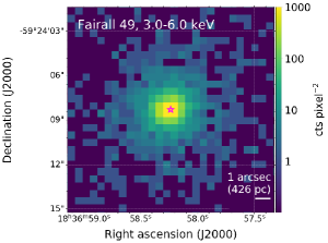
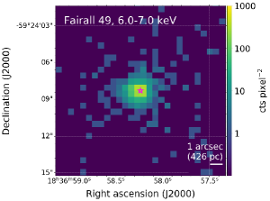
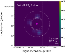
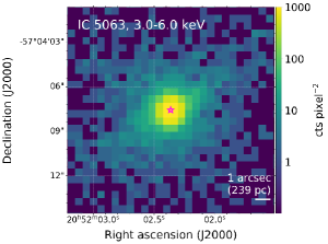
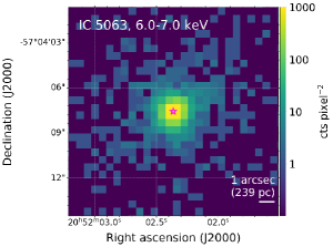
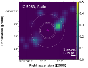
Figure 24: Continued.

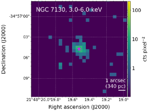
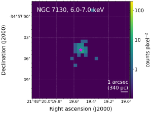
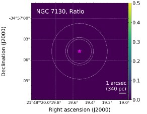
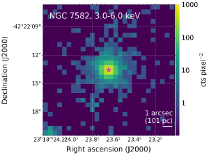
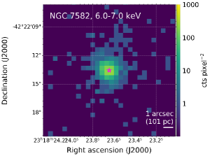
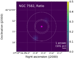
Figure 24: Continued.

Appendix E Spectra of CO($J$=2–1) emission

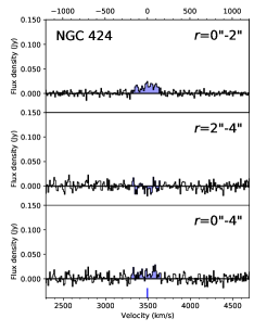
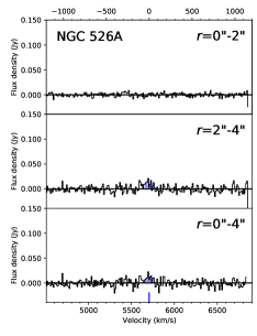
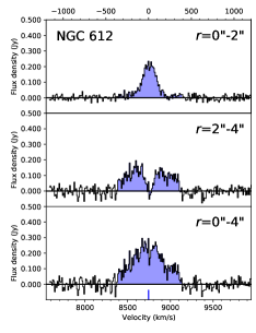
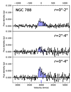
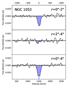
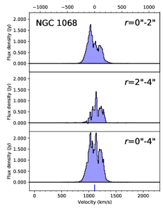
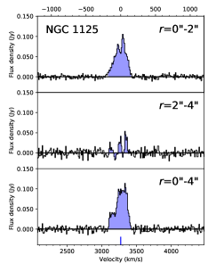
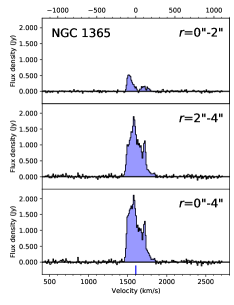
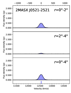
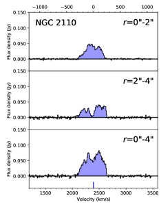
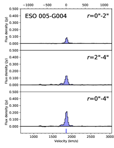
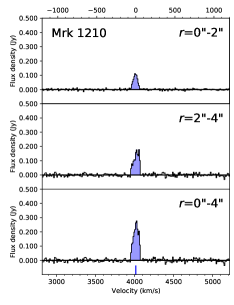
Figure 25: Spectra around the CO($J$=2–1) emission centered at flux-weighted velocities indicated by blue vertical lines. Each figure shows three spectra taken from a nuclear ($<$ 2″) region, an external (2″–4″) region, and an entire ($<$ 4″) region, from top to bottom. The CO($J$=2–1) luminosities in Table 4 are derived from the blue shaded areas.

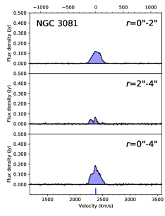
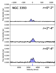
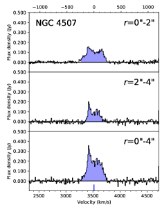
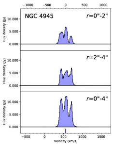
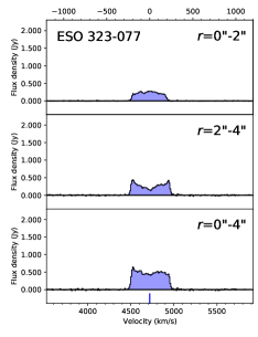
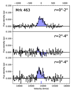
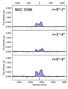
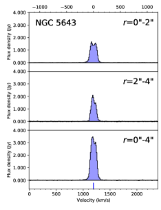
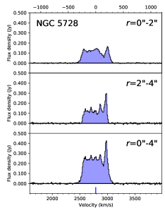
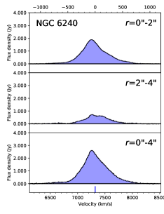
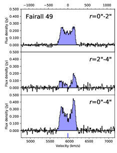
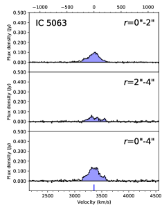
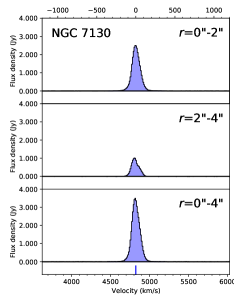
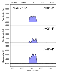
Figure 25: Continued.

Appendix F CO($J$=2–1) images

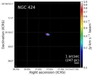
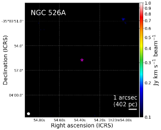
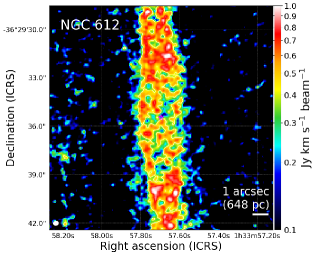
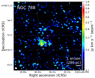
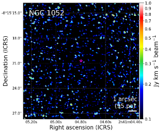
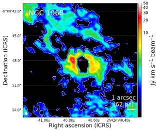
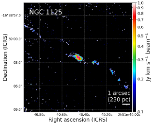
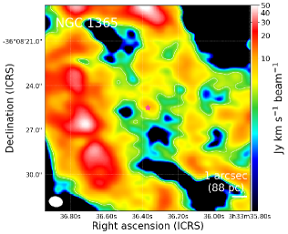
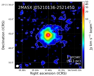
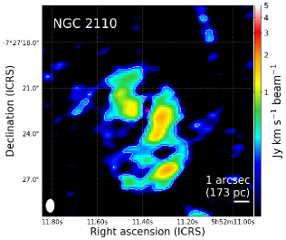
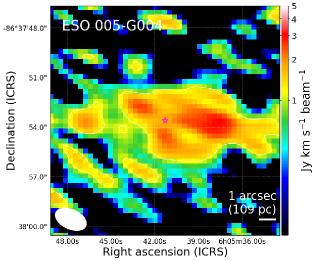
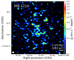
Figure 26: Moment 0 maps of the CO($J$=2–1) emission. North is up and east is left. White contours are plotted to indicate 5$\sigma$, where 1$\sigma$ flux densities in units of Jy km s^-1 beam^-1 are listed in the column (8) of Table 3. In addition, beam sizes are plotted at the bottom-left corners.

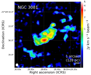
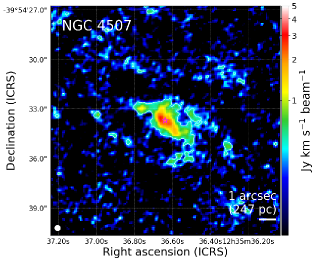
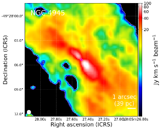
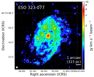
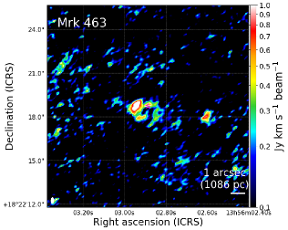
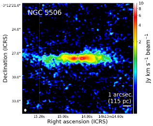
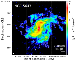
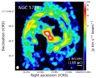
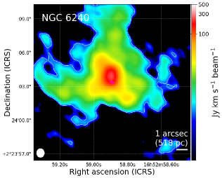
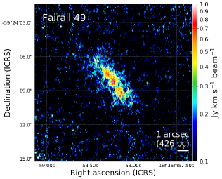
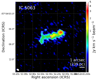
Figure 26: Continued.

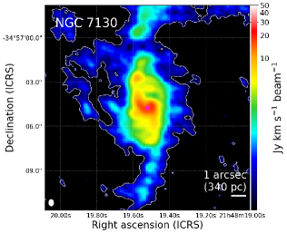
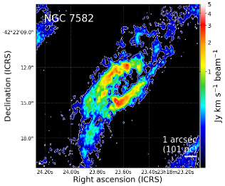
Figure 26: Continued.

References

- Asakura et al. (2020) Asakura, K., Hayashida, K., Hanasaka, T., et al. 2020, in Society of Photo-Optical Instrumentation Engineers (SPIE) Conference Series, Vol. 11444, Society of Photo-Optical Instrumentation Engineers (SPIE) Conference Series, 114441D, doi: 10.1117/12.2560772
- Baek et al. (2019) Baek, J., Chung, A., Schawinski, K., et al. 2019, MNRAS, 488, 4317, doi: 10.1093/mnras/stz1995
- Baumgartner et al. (2013) Baumgartner, W. H., Tueller, J., Markwardt, C. B., et al. 2013, ApJS, 207, 19, doi: 10.1088/0067-0049/207/2/19
- Behar et al. (2015) Behar, E., Baldi, R. D., Laor, A., et al. 2015, MNRAS, 451, 517, doi: 10.1093/mnras/stv988
- Behar et al. (2018) Behar, E., Vogel, S., Baldi, R. D., Smith, K. L., & Mushotzky, R. F. 2018, MNRAS, 478, 399, doi: 10.1093/mnras/sty850
- Bianchi et al. (2008) Bianchi, S., Chiaberge, M., Piconcelli, E., Guainazzi, M., & Matt, G. 2008, MNRAS, 386, 105, doi: 10.1111/j.1365-2966.2008.13078.x
- Bianchi & Guainazzi (2007) Bianchi, S., & Guainazzi, M. 2007, in American Institute of Physics Conference Series, Vol. 924, The Multicolored Landscape of Compact Objects and Their Explosive Origins, ed. T. di Salvo, G. L. Israel, L. Piersant, L. Burderi, G. Matt, A. Tornambe, & M. T. Menna, 822–829, doi: 10.1063/1.2774948
- Bianchi et al. (2001) Bianchi, S., Matt, G., & Iwasawa, K. 2001, MNRAS, 322, 669, doi: 10.1046/j.1365-8711.2001.04156.x
- Bigiel et al. (2015) Bigiel, F., Leroy, A. K., Blitz, L., et al. 2015, ApJ, 815, 103, doi: 10.1088/0004-637X/815/2/103
- Boller et al. (2003) Boller, T., Keil, R., Hasinger, G., et al. 2003, A&A, 411, 63, doi: 10.1051/0004-6361:20031217
- Combes et al. (2019) Combes, F., García-Burillo, S., Audibert, A., et al. 2019, A&A, 623, A79, doi: 10.1051/0004-6361/201834560
- Croton et al. (2006) Croton, D. J., Springel, V., White, S. D. M., et al. 2006, MNRAS, 365, 11, doi: 10.1111/j.1365-2966.2005.09675.x
- Di Matteo et al. (2005) Di Matteo, T., Springel, V., & Hernquist, L. 2005, Nature, 433, 604, doi: 10.1038/nature03335
- Elvis et al. (1994) Elvis, M., Wilkes, B. J., McDowell, J. C., et al. 1994, ApJS, 95, 1, doi: 10.1086/192093
- Fabbiano et al. (2017) Fabbiano, G., Elvis, M., Paggi, A., et al. 2017, ApJ, 842, L4, doi: 10.3847/2041-8213/aa7551
- Fabbiano et al. (2019) Fabbiano, G., Paggi, A., & Elvis, M. 2019, ApJ, 876, L18, doi: 10.3847/2041-8213/ab1c63
- Fabbiano et al. (2018a) Fabbiano, G., Paggi, A., Karovska, M., et al. 2018a, ApJ, 855, 131, doi: 10.3847/1538-4357/aab1f4
- Fabbiano et al. (2018b) —. 2018b, ApJ, 865, 83, doi: 10.3847/1538-4357/aadc5d
- Fabbiano et al. (2020) —. 2020, ApJ, 902, 49, doi: 10.3847/1538-4357/abb5ad
- Fabian (1977) Fabian, A. C. 1977, Nature, 269, 672, doi: 10.1038/269672a0
- Fabian et al. (2009) Fabian, A. C., Vasudevan, R. V., Mushotzky, R. F., Winter, L. M., & Reynolds, C. S. 2009, MNRAS, 394, L89, doi: 10.1111/j.1745-3933.2009.00617.x
- Feruglio et al. (2020) Feruglio, C., Fabbiano, G., Bischetti, M., et al. 2020, ApJ, 890, 29, doi: 10.3847/1538-4357/ab67bd
- Gao & Solomon (2004) Gao, Y., & Solomon, P. M. 2004, ApJ, 606, 271, doi: 10.1086/382999
- García-Burillo et al. (2010) García-Burillo, S., Usero, A., Fuente, A., et al. 2010, A&A, 519, A2, doi: 10.1051/0004-6361/201014539
- García-Burillo et al. (2014) García-Burillo, S., Combes, F., Usero, A., et al. 2014, A&A, 567, A125, doi: 10.1051/0004-6361/201423843
- Garcia-Burillo et al. (2021) Garcia-Burillo, S., Alonso-Herrero, A., Ramos Almeida, C., et al. 2021, arXiv e-prints, arXiv:2104.10227. https://arxiv.org/abs/2104.10227
- Garmire et al. (2003) Garmire, G. P., Bautz, M. W., Ford, P. G., Nousek, J. A., & Ricker, George R., J. 2003, in Society of Photo-Optical Instrumentation Engineers (SPIE) Conference Series, Vol. 4851, Proc. SPIE, ed. J. E. Truemper & H. D. Tananbaum, 28–44, doi: 10.1117/12.461599
- Gebhardt et al. (2000) Gebhardt, K., Bender, R., Bower, G., et al. 2000, ApJ, 539, L13, doi: 10.1086/312840
- Gehrels (1986) Gehrels, N. 1986, ApJ, 303, 336, doi: 10.1086/164079
- Gómez-Guijarro et al. (2017) Gómez-Guijarro, C., González-Martín, O., Ramos Almeida, C., Rodríguez-Espinosa, J. M., & Gallego, J. 2017, MNRAS, 469, 2720, doi: 10.1093/mnras/stx1037
- Gültekin et al. (2009) Gültekin, K., Richstone, D. O., Gebhardt, K., et al. 2009, ApJ, 698, 198, doi: 10.1088/0004-637X/698/1/198
- Gupta et al. (2021) Gupta, K. K., Ricci, C., Tortosa, A., et al. 2021, MNRAS, 504, 428, doi: 10.1093/mnras/stab839
- Hayashida et al. (2018) Hayashida, K., Kawabata, T., Hanasaka, T., et al. 2018, in Society of Photo-Optical Instrumentation Engineers (SPIE) Conference Series, Vol. 10699, Space Telescopes and Instrumentation 2018: Ultraviolet to Gamma Ray, ed. J.-W. A. den Herder, S. Nikzad, & K. Nakazawa, 106990U, doi: 10.1117/12.2314181
- Henkel et al. (2018) Henkel, C., Mühle, S., Bendo, G., et al. 2018, A&A, 615, A155, doi: 10.1051/0004-6361/201732174
- Hickox & Alexander (2018) Hickox, R. C., & Alexander, D. M. 2018, ARA&A, 56, 625, doi: 10.1146/annurev-astro-081817-051803
- Hocuk & Spaans (2010) Hocuk, S., & Spaans, M. 2010, A&A, 522, A24, doi: 10.1051/0004-6361/201015055
- Hocuk & Spaans (2011) —. 2011, A&A, 536, A41, doi: 10.1051/0004-6361/201117431
- Hori et al. (2018) Hori, T., Shidatsu, M., Ueda, Y., et al. 2018, ApJS, 235, 7, doi: 10.3847/1538-4365/aaa89c
- Ichikawa et al. (2019) Ichikawa, K., Ricci, C., Ueda, Y., et al. 2019, ApJ, 870, 31, doi: 10.3847/1538-4357/aaef8f
- Imanishi et al. (2009) Imanishi, M., Nakanishi, K., Tamura, Y., & Peng, C.-H. 2009, AJ, 137, 3581, doi: 10.1088/0004-6256/137/3/3581
- Inoue & Doi (2018) Inoue, Y., & Doi, A. 2018, ApJ, 869, 114, doi: 10.3847/1538-4357/aaeb95
- Isobe et al. (1990) Isobe, T., Feigelson, E. D., Akritas, M. G., & Babu, G. J. 1990, ApJ, 364, 104, doi: 10.1086/169390
- Iwasawa et al. (1997) Iwasawa, K., Fabian, A. C., & Matt, G. 1997, MNRAS, 289, 443, doi: 10.1093/mnras/289.2.443
- Iyomoto et al. (1996) Iyomoto, N., Makishima, K., Fukazawa, Y., et al. 1996, PASJ, 48, 231, doi: 10.1093/pasj/48.2.231
- Izumi et al. (2016a) Izumi, T., Kawakatu, N., & Kohno, K. 2016a, ApJ, 827, 81, doi: 10.3847/0004-637X/827/1/81
- Izumi et al. (2018) Izumi, T., Wada, K., Fukushige, R., Hamamura, S., & Kohno, K. 2018, ApJ, 867, 48, doi: 10.3847/1538-4357/aae20b
- Izumi et al. (2016b) Izumi, T., Kohno, K., Aalto, S., et al. 2016b, ApJ, 818, 42, doi: 10.3847/0004-637X/818/1/42
- Izumi et al. (2020) Izumi, T., Nguyen, D. D., Imanishi, M., et al. 2020, ApJ, 898, 75, doi: 10.3847/1538-4357/ab9cb1
- Kalberla et al. (2005) Kalberla, P. M. W., Burton, W. B., Hartmann, D., et al. 2005, A&A, 440, 775, doi: 10.1051/0004-6361:20041864
- Kameno et al. (2020) Kameno, S., Sawada-Satoh, S., Impellizzeri, C. M. V., et al. 2020, ApJ, 895, 73, doi: 10.3847/1538-4357/ab8bd6
- Kawamuro et al. (2019a) Kawamuro, T., Izumi, T., & Imanishi, M. 2019a, PASJ, 71, 68, doi: 10.1093/pasj/psz045
- Kawamuro et al. (2020) Kawamuro, T., Izumi, T., Onishi, K., et al. 2020, ApJ, 895, 135, doi: 10.3847/1538-4357/ab8b62
- Kawamuro et al. (2019b) Kawamuro, T., Ueda, Y., Ichikawa, K., et al. 2019b, ApJ, 881, 48, doi: 10.3847/1538-4357/ab2bf6
- Kawamuro et al. (2016a) Kawamuro, T., Ueda, Y., Tazaki, F., Ricci, C., & Terashima, Y. 2016a, ApJS, 225, 14, doi: 10.3847/0067-0049/225/1/14
- Kawamuro et al. (2013) Kawamuro, T., Ueda, Y., Tazaki, F., & Terashima, Y. 2013, ApJ, 770, 157, doi: 10.1088/0004-637X/770/2/157
- Kawamuro et al. (2016b) Kawamuro, T., Ueda, Y., Tazaki, F., Terashima, Y., & Mushotzky, R. 2016b, ApJ, 831, 37, doi: 10.3847/0004-637X/831/1/37
- Kawamuro et al. (2018) Kawamuro, T., Ueda, Y., Shidatsu, M., et al. 2018, ApJS, 238, 32, doi: 10.3847/1538-4365/aad1ef
- Kohno (2005) Kohno, K. 2005, in American Institute of Physics Conference Series, Vol. 783, The Evolution of Starbursts, ed. S. Hüttmeister, E. Manthey, D. Bomans, & K. Weis, 203–208, doi: 10.1063/1.2034987
- Komossa et al. (2003) Komossa, S., Burwitz, V., Hasinger, G., et al. 2003, ApJ, 582, L15, doi: 10.1086/346145
- Kormendy & Ho (2013) Kormendy, J., & Ho, L. C. 2013, ARA&A, 51, 511, doi: 10.1146/annurev-astro-082708-101811
- Koss et al. (2017) Koss, M., Trakhtenbrot, B., Ricci, C., et al. 2017, ApJ, 850, 74, doi: 10.3847/1538-4357/aa8ec9
- Koss et al. (2021) Koss, M. J., Strittmatter, B., Lamperti, I., et al. 2021, ApJS, 252, 29, doi: 10.3847/1538-4365/abcbfe
- Koyama et al. (1996) Koyama, K., Maeda, Y., Sonobe, T., et al. 1996, PASJ, 48, 249, doi: 10.1093/pasj/48.2.249
- Koyama et al. (2007) Koyama, K., Inui, T., Hyodo, Y., et al. 2007, PASJ, 59, 221, doi: 10.1093/pasj/59.sp1.S221
- Krips et al. (2008) Krips, M., Neri, R., García-Burillo, S., et al. 2008, ApJ, 677, 262, doi: 10.1086/527367
- Krolik & Kallman (1984) Krolik, J. H., & Kallman, T. R. 1984, ApJ, 286, 366, doi: 10.1086/162608
- Krolik & Kallman (1987) —. 1987, ApJ, 320, L5, doi: 10.1086/184966
- Krumholz & Tan (2007) Krumholz, M. R., & Tan, J. C. 2007, ApJ, 654, 304, doi: 10.1086/509101
- Laha et al. (2018) Laha, S., Guainazzi, M., Piconcelli, E., et al. 2018, ApJ, 868, 10, doi: 10.3847/1538-4357/aae390
- LaMassa et al. (2012) LaMassa, S. M., Heckman, T. M., & Ptak, A. 2012, ApJ, 758, 82, doi: 10.1088/0004-637X/758/2/82
- LaMassa et al. (2017) LaMassa, S. M., Yaqoob, T., Levenson, N. A., et al. 2017, ApJ, 835, 91, doi: 10.3847/1538-4357/835/1/91
- Lamperti et al. (2017) Lamperti, I., Koss, M., Trakhtenbrot, B., et al. 2017, MNRAS, 467, 540, doi: 10.1093/mnras/stx055
- Ma et al. (2020) Ma, J., Elvis, M., Fabbiano, G., et al. 2020, ApJ, 900, 164, doi: 10.3847/1538-4357/abacbe
- Magdziarz & Zdziarski (1995) Magdziarz, P., & Zdziarski, A. A. 1995, MNRAS, 273, 837, doi: 10.1093/mnras/273.3.837
- Magorrian et al. (1998) Magorrian, J., Tremaine, S., Richstone, D., et al. 1998, AJ, 115, 2285, doi: 10.1086/300353
- Maloney et al. (1996) Maloney, P. R., Hollenbach, D. J., & Tielens, A. G. G. M. 1996, ApJ, 466, 561, doi: 10.1086/177532
- Marconi & Hunt (2003) Marconi, A., & Hunt, L. K. 2003, ApJ, 589, L21, doi: 10.1086/375804
- Marconi et al. (2004) Marconi, A., Risaliti, G., Gilli, R., et al. 2004, MNRAS, 351, 169, doi: 10.1111/j.1365-2966.2004.07765.x
- Marinucci et al. (2017) Marinucci, A., Bianchi, S., Fabbiano, G., et al. 2017, MNRAS, 470, 4039, doi: 10.1093/mnras/stx1551
- Marinucci et al. (2013) Marinucci, A., Miniutti, G., Bianchi, S., Matt, G., & Risaliti, G. 2013, MNRAS, 436, 2500, doi: 10.1093/mnras/stt1759
- Marinucci et al. (2012) Marinucci, A., Risaliti, G., Wang, J., et al. 2012, MNRAS, 423, L6, doi: 10.1111/j.1745-3933.2012.01232.x
- Masini et al. (2016) Masini, A., Comastri, A., Baloković, M., et al. 2016, A&A, 589, A59, doi: 10.1051/0004-6361/201527689
- Matt et al. (2004) Matt, G., Bianchi, S., Guainazzi, M., & Molendi, S. 2004, A&A, 414, 155, doi: 10.1051/0004-6361:20031635
- McMullin et al. (2007) McMullin, J. P., Waters, B., Schiebel, D., Young, W., & Golap, K. 2007, Astronomical Society of the Pacific Conference Series, Vol. 376, CASA Architecture and Applications, ed. R. A. Shaw, F. Hill, & D. J. Bell, 127
- Meijerink & Spaans (2005) Meijerink, R., & Spaans, M. 2005, A&A, 436, 397, doi: 10.1051/0004-6361:20042398
- Meijerink et al. (2007) Meijerink, R., Spaans, M., & Israel, F. P. 2007, A&A, 461, 793, doi: 10.1051/0004-6361:20066130
- Mineo et al. (2012) Mineo, S., Gilfanov, M., & Sunyaev, R. 2012, MNRAS, 419, 2095, doi: 10.1111/j.1365-2966.2011.19862.x
- Miyamoto et al. (2018) Miyamoto, Y., Seta, M., Nakai, N., et al. 2018, PASJ, 70, L1, doi: 10.1093/pasj/psy016
- Monje et al. (2011) Monje, R. R., Blain, A. W., & Phillips, T. G. 2011, ApJS, 195, 23, doi: 10.1088/0067-0049/195/2/23
- Murakami et al. (2000) Murakami, H., Koyama, K., Sakano, M., Tsujimoto, M., & Maeda, Y. 2000, ApJ, 534, 283, doi: 10.1086/308717
- Murphy & Yaqoob (2009) Murphy, K. D., & Yaqoob, T. 2009, MNRAS, 397, 1549, doi: 10.1111/j.1365-2966.2009.15025.x
- Mushotzky et al. (2019) Mushotzky, R., Aird, J., Barger, A. J., et al. 2019, in Bulletin of the American Astronomical Society, Vol. 51, 107. https://arxiv.org/abs/1903.04083
- Mushotzky et al. (2014) Mushotzky, R. F., Shimizu, T. T., Meléndez, M., & Koss, M. 2014, ApJ, 781, L34, doi: 10.1088/2041-8205/781/2/L34
- Nakata et al. (2021) Nakata, R., Hayashida, K., Noda, H., et al. 2021, PASJ, doi: 10.1093/pasj/psab001
- Nemmen et al. (2006) Nemmen, R. S., Storchi-Bergmann, T., Yuan, F., et al. 2006, ApJ, 643, 652, doi: 10.1086/500571
- Nobukawa et al. (2010) Nobukawa, M., Koyama, K., Tsuru, T. G., Ryu, S. G., & Tatischeff, V. 2010, PASJ, 62, 423, doi: 10.1093/pasj/62.2.423
- Noguchi et al. (2010) Noguchi, K., Terashima, Y., Ishino, Y., et al. 2010, ApJ, 711, 144, doi: 10.1088/0004-637X/711/1/144
- Ogawa et al. (2021) Ogawa, S., Ueda, Y., Tanimoto, A., & Yamada, S. 2021, ApJ, 906, 84, doi: 10.3847/1538-4357/abccce
- Ogle et al. (2003) Ogle, P. M., Brookings, T., Canizares, C. R., Lee, J. C., & Marshall, H. L. 2003, A&A, 402, 849, doi: 10.1051/0004-6361:20021647
- Ponti et al. (2010) Ponti, G., Terrier, R., Goldwurm, A., Belanger, G., & Trap, G. 2010, ApJ, 714, 732, doi: 10.1088/0004-637X/714/1/732
- Predehl & Schmitt (1995) Predehl, P., & Schmitt, J. H. M. M. 1995, A&A, 500, 459
- Puccetti et al. (2016) Puccetti, S., Comastri, A., Bauer, F. E., et al. 2016, A&A, 585, A157, doi: 10.1051/0004-6361/201527189
- Ramakrishnan et al. (2019) Ramakrishnan, V., Nagar, N. M., Finlez, C., et al. 2019, MNRAS, 487, 444, doi: 10.1093/mnras/stz1244
- Ricci et al. (2014) Ricci, C., Ueda, Y., Paltani, S., et al. 2014, MNRAS, 441, 3622, doi: 10.1093/mnras/stu735
- Ricci et al. (2017a) Ricci, C., Trakhtenbrot, B., Koss, M. J., et al. 2017a, ApJS, 233, 17, doi: 10.3847/1538-4365/aa96ad
- Ricci et al. (2017b) —. 2017b, Nature, 549, 488, doi: 10.1038/nature23906
- Rosario et al. (2019) Rosario, D. J., Togi, A., Burtscher, L., et al. 2019, ApJ, 875, L8, doi: 10.3847/2041-8213/ab1262
- Rose et al. (2019) Rose, T., Edge, A. C., Combes, F., et al. 2019, MNRAS, 485, 229, doi: 10.1093/mnras/stz406
- Sandstrom et al. (2013) Sandstrom, K. M., Leroy, A. K., Walter, F., et al. 2013, ApJ, 777, 5, doi: 10.1088/0004-637X/777/1/5
- Shangguan et al. (2020) Shangguan, J., Ho, L. C., Bauer, F. E., Wang, R., & Treister, E. 2020, ApJ, 899, 112, doi: 10.3847/1538-4357/aba8a1
- Shimizu et al. (2017) Shimizu, T. T., Mushotzky, R. F., Meléndez, M., et al. 2017, MNRAS, 466, 3161, doi: 10.1093/mnras/stw3268
- Smith et al. (2020) Smith, K. L., Mushotzky, R. F., Koss, M., et al. 2020, MNRAS, 492, 4216, doi: 10.1093/mnras/stz3608
- Solomon & Vanden Bout (2005) Solomon, P. M., & Vanden Bout, P. A. 2005, ARA&A, 43, 677, doi: 10.1146/annurev.astro.43.051804.102221
- Soltan (1982) Soltan, A. 1982, MNRAS, 200, 115, doi: 10.1093/mnras/200.1.115
- Tanimoto et al. (2016) Tanimoto, A., Ueda, Y., Kawamuro, T., & Ricci, C. 2016, PASJ, 68, S26, doi: 10.1093/pasj/psw008
- Tanimoto et al. (2018) Tanimoto, A., Ueda, Y., Kawamuro, T., et al. 2018, ApJ, 853, 146, doi: 10.3847/1538-4357/aaa47c
- Tatischeff et al. (2012) Tatischeff, V., Decourchelle, A., & Maurin, G. 2012, A&A, 546, A88, doi: 10.1051/0004-6361/201219016
- The Lynx Team (2018) The Lynx Team. 2018, arXiv e-prints, arXiv:1809.09642. https://arxiv.org/abs/1809.09642
- Torrejón et al. (2010) Torrejón, J. M., Schulz, N. S., Nowak, M. A., & Kallman, T. R. 2010, ApJ, 715, 947, doi: 10.1088/0004-637X/715/2/947
- Treister et al. (2018) Treister, E., Privon, G. C., Sartori, L. F., et al. 2018, ApJ, 854, 83, doi: 10.3847/1538-4357/aaa963
- Treister et al. (2020) Treister, E., Messias, H., Privon, G. C., et al. 2020, ApJ, 890, 149, doi: 10.3847/1538-4357/ab6b28
- Ueda et al. (2014) Ueda, Y., Akiyama, M., Hasinger, G., Miyaji, T., & Watson, M. G. 2014, ApJ, 786, 104, doi: 10.1088/0004-637X/786/2/104
- Ursini et al. (2018) Ursini, F., Bassani, L., Panessa, F., et al. 2018, MNRAS, 474, 5684, doi: 10.1093/mnras/stx3159
- Valinia et al. (2000) Valinia, A., Tatischeff, V., Arnaud, K., Ebisawa, K., & Ramaty, R. 2000, ApJ, 543, 733, doi: 10.1086/317133
- Venturi et al. (2017) Venturi, G., Marconi, A., Mingozzi, M., et al. 2017, Frontiers in Astronomy and Space Sciences, 4, 46, doi: 10.3389/fspas.2017.00046
- Viti et al. (2014) Viti, S., García-Burillo, S., Fuente, A., et al. 2014, A&A, 570, A28, doi: 10.1051/0004-6361/201424116
- Wang et al. (2009) Wang, J., Fabbiano, G., Elvis, M., et al. 2009, ApJ, 694, 718, doi: 10.1088/0004-637X/694/2/718
- Wilms et al. (2000) Wilms, J., Allen, A., & McCray, R. 2000, ApJ, 542, 914, doi: 10.1086/317016
- Xu et al. (2016) Xu, W., Liu, Z., Gou, L., & Liu, J. 2016, MNRAS, 455, L26, doi: 10.1093/mnrasl/slv148
- Yamada et al. (2018) Yamada, S., Ueda, Y., Oda, S., et al. 2018, ApJ, 858, 106, doi: 10.3847/1538-4357/aabacb
- Yamada et al. (2020) Yamada, S., Ueda, Y., Tanimoto, A., et al. 2020, ApJ, 897, 107, doi: 10.3847/1538-4357/ab94b1
- Yamada (1994) Yamada, T. 1994, ApJ, 423, L27, doi: 10.1086/187227
- Yan et al. (2021) Yan, W., Hickox, R. C., Chen, C.-T. J., et al. 2021, arXiv e-prints, arXiv:2104.10702. https://arxiv.org/abs/2104.10702
- Younes et al. (2019) Younes, G., Ptak, A., Ho, L. C., et al. 2019, ApJ, 870, 73, doi: 10.3847/1538-4357/aaf38b
- Young et al. (2001) Young, A. J., Wilson, A. S., & Shopbell, P. L. 2001, ApJ, 556, 6, doi: 10.1086/321561
- Yusef-Zadeh et al. (2002) Yusef-Zadeh, F., Law, C., Wardle, M., et al. 2002, ApJ, 570, 665, doi: 10.1086/340058
- Yusef-Zadeh et al. (2007) Yusef-Zadeh, F., Muno, M., Wardle, M., & Lis, D. C. 2007, ApJ, 656, 847, doi: 10.1086/510663