Assessment of diffuse-interface methods for compressible
multiphase fluid flows and elastic-plastic deformation in solids

Abstract

This work describes three diffuse-interface methods for the simulation of immiscible, compressible multiphase fluid flows and elastic-plastic deformation in solids. The first method is the localized-artificial-diffusivity approach of Cook (2007), Subramaniam et al. (2018), and Adler and Lele (2019), in which artificial diffusion terms are added to the individual phase mass fraction transport equations and are coupled with the other conservation equations. The second method is the gradient-form approach that is based on the quasi-conservative method of Shukla et al. (2010), in which the diffusion and sharpening terms (together called regularization terms) are added to the individual phase volume fraction transport equations and are coupled with the other conservation equations (Tiwari et al., 2013). The third approach is the divergence-form approach that is based on the fully conservative method of Jain et al. (2020), in which the regularization terms are added to the individual phase volume fraction transport equations and are coupled with the other conservation equations. In the present study, all three diffuse-interface methods are used in conjunction with a four-equation, multicomponent mixture model, in which pressure and temperature equilibria are assumed among the various phases.

The primary objective of this work is to compare these three methods in terms of their ability to: maintain constant interface thickness throughout the simulation; conserve mass, momentum, and energy; and maintain accurate interface shape for long-time integration. The second objective of this work is to consistently extend these methods to model interfaces between solid materials with strength. To assess and compare the methods, they are used to simulate a wide variety of problems, including (1) advection of an air bubble in water, (2) shock interaction with a helium bubble in air, (3) shock interaction and the collapse of an air bubble in water, and (4) Richtmyer–Meshkov instability of a copper–aluminum interface. The current work focuses on comparing these methods in the limit of relatively coarse grid resolution, which illustrates the true performance of these methods. This is because it is rarely practical to use hundreds of grid points to resolve a single bubble or drop in large-scale simulations of engineering interest.

1 Introduction

Compressible multiphase fluid flow and multiphase elastic-plastic deformation of solid materials with strength are important phenomena in many engineering applications, including shock compression of condensed matter, detonations and shock-material-interface interactions, impact welding, high-speed fuel atomization and combustion, and cavitation and bubble collapse motivated by both mechanical and biomedical systems. In this work, we are concerned with the numerical modeling of multiphase systems, i.e., those systems that involve two or more phases of gas, liquid, or solid in the domain. The numerical simulation of these multiphase systems presents several new challenges in addition to those associated with analogous single-phase simulations. These modeling complications include but are not limited to (1) representing the phase interface on an Eulerian grid; (2) resolving discontinuities in quantities at the interface, especially for high-density ratios; (3) maintaining conservation of (a) the mass of each phase, (b) the mixture momentum, and (c) the total energy of the system; and (4) achieving an accurate mixture representation of the interface for maintaining thermodynamic equilibria. Hence, the numerical modeling of multiphase compressible fluid flows and deformation of solid materials with strength are still an active area of research.

With these numerical challenges in mind, we choose to pursue the single-fluid approach (Kataoka, 1986), in which a single set of equations is solved to describe all of the phases in the domain, as opposed to a multi-fluid approach, which requires solving a separate set of equations for each of the phases. We are presented with various choices in terms of the system of equations that can be used to represent a compressible multiphase system. In this work, we employ a multicomponent system of equations (a four-equation model) that assumes spatially local pressure and temperature equilibria, including at locations within the diffuse material interface (Shyue, 1998, Venkateswaran et al., 2002, Marquina and Mulet, 2003, Cook, 2009). Relaxing the assumption of temperature equilibrium, Allaire et al. (2002) and Kapila et al. (2001) developed the five-equation model that has proven successful for a variety of applications with high density ratios, strong compressibility effects, and phases with disparate equations of state (EOS), and has been widely adopted for the simulation of compressible two-phase flows (Shukla et al., 2010, So et al., 2012, Ansari and Daramizadeh, 2013, Shukla, 2014, Coralic and Colonius, 2014, Tiwari et al., 2013, Perigaud and Saurel, 2005, Wong and Lele, 2017, Chiapolino et al., 2017, Garrick et al., 2017a, b, Jain et al., 2018, 2020). Finally, there are six- and seven-equation models that are more general and include more non-equilibrium effects but are not as widely used for the simulation of two-phase flows (Yeom and Chang, 2013, Baer and Nunziato, 1986, Sainsaulieu, 1995, Saurel and Abgrall, 1999).

For representing the interface on an Eulerian grid, we use an interface-capturing method, as opposed to an interface-tracking method, due to the natural ability of the former method to simulate dynamic creation of interfaces and topological changes (Mirjalili et al., 2017). Interface-capturing methods can be classified into sharp-interface and diffuse-interface methods. In this work, we choose to use diffuse-interface methods for modeling the interface between compressible materials (Saurel and Pantano, 2018). This choice is due to the natural advantages that the diffuse-interface methods offer over the sharp-interface methods, such as ease of representation of the interface, low cost, good conservation properties, and parallel scalability.

Historically, diffuse-interface methods for compressible flows involved modeling the interface implicity, i.e., with no explicit interface capturing through regularization/reconstruction. These methods can be classified as implicit diffuse-interface methods. These methods assume that the underlying numerical methods are capable of handling the material interfaces, a concept similar to implicit large-eddy simulation. One challenge with the implicit diffuse-interface capturing of material interfaces is that the interface tends to diffuse over time. Unlike shock waves, in which the convective characteristics sharpen the shock over time, material interfaces (like contact discontinuities) do not sharpen naturally; therefore, modeling material interfaces requires an active balance between interface sharpening and diffusion to maintain an appropriate interface thickness over time. Therefore, in the present work, the focus is on explicit diffuse-interface methods. These methods explicitly model the interface using the interface regularization/reconstruction techniques.

This paper explores three explicit diffuse-interface methods that are representative of the different approaches for this problem and possesses unique characteristics. The first approach (referred to as the LAD approach) is based on the localized-artificial-diffusivity (LAD) method (Cook, 2007, Subramaniam et al., 2018, Adler and Lele, 2019), in which localized, nonlinear diffusion terms are added to the individual phase mass transport equations and coupled with the other conservation equations. This method conserves the mass of individual phases, mixture momentum, and total energy of the system due to the conservative nature of the diffusion terms added to the system of equations and results in no net mixture-mass transport. This method is primarily motivated by applications involving miscible, multicomponent, single-phase flows, but it has been successfully adapted for multiphase flow applications. The idea behind this approach is to effectively add species diffusion in the selected regions of the domain to properly resolve the interface on the grid and to prevent oscillations due to discontinuities in the phase mass equations. High-order compact derivative schemes can be used to discretize the added diffusion terms without resulting in distortion of the shape of the interface over long-duration time advancement. However, one drawback of this approach is that the interface thickness increases with time due to the lack of sharpening fluxes that act against the diffusion. This method is therefore most effective for problems in which the interface is in compression (such as shock/material-interface interactions with normal alignment). However, the deficiency of this method due to the lack of a sharpening term is evident for applications in which the interface between immiscible materials undergoes shear or expansion/tension. LAD formulations have also been examined in the context of five-equation models, in which localized diffusion is also added to the volume fraction transport equation (Aslani and Regele, 2018).

The second approach (referred to as the gradient-form approach) is based on the quasi-conservative method proposed by Shukla et al. (2010), in which diffusion and sharpening terms (together called regularization terms) are added for the individual phase volume fraction transport equations and coupled with the other conservation equations (Tiwari et al., 2013). This method only approximately conserves the mass of individual phases, mixture momentum, and total energy of the system due to the non-conservative nature of the regularization terms added to the system of equations. In contrast to the LAD approach, this method can result in net mixture-mass transport, which can sharpen or diffuse the mixture density; depending on the application, this may be an advantageous or disadvantageous property. The primary advantage of this method is that the regularization terms are insensitive to the method of discretization; they can be discretized using high-order compact derivative schemes without distorting the shape of the interface over long-duration time advancement. However, the non-conservative nature of this approach results in poor performance of the method for certain applications. For example, premature topological changes and unphysical interface behavior can be observed when the interfaces are poorly resolved (exacerbating the conservation error) and subjected to shocks that are not aligned with the interface.

The third approach (referred to as the divergence-form approach) is based on the fully conservative method proposed by Jain et al. (2020), in which diffusion and sharpening terms are added to the individual phase volume fraction transport equations and coupled with the other conservation equations. This method conserves the mass of individual phases, mixture momentum, and total energy of the system due to the conservative nature of the regularization terms added to the system of equations. Similar to the gradient-form approach and in contrast to the LAD approach, this method can result in net mixture-mass transport, which can sharpen or diffuse the mixture density. The primary challenge of this method is that one needs to be careful with the choice of discretization used for the regularization terms. Using a second-order finite-volume scheme (in which the nonlinear fluxes are formed on the faces), Jain et al. (2020) showed that a discrete balance between the diffusion and sharpening terms is achieved, thereby eliminating the spurious behavior that was discussed by Shukla et al. (2010). The idea behind this is similar to the use of the balanced-force algorithm (Francois et al., 2006, Mencinger and Žun, 2007) for the implementation of the surface-tension forces, in which a discrete balance between the pressure and surface-tension forces is necessary to eliminate the spurious velocity around the interface. The current study also demonstrates that appropriately crafted higher-order schemes may be used to effectively discretize the regularization terms. This method is free of premature topological changes and unphysical interface behavior present with the previous approach. However, due to the method of discretization, the anisotropy of the derivative scheme can more significantly distort the shape of the material interface over long-duration time advancement in comparison to the gradient-form approach; the severity of this problem is significantly reduced when using higher-order schemes.

For all the three diffuse-interface methods considered in this work, it is important to include physically consistent corrections, associated with the interface regularization process, in each of the governing equations. For example, Cook (2009), Tiwari et al. (2013), and Jain et al. (2020) discuss physically consistent regularization terms for the LAD, gradient-form, and divergence-form approaches, respectively. The physically consistent regularization terms of Cook (2009), Tiwari et al. (2013), and Jain et al. (2020) are derived in such a way that the regularization terms do not spuriously contribute to the kinetic energy and entropy of the system. This significantly improves the stability of the simulation, especially for flows with high density ratios. However, discrete conservation of kinetic energy and entropy is needed to show the stability of the methods for high-Reynolds-number turbulent flows (Jain and Moin, 2020).

We employ a fully Eulerian method for modeling the deformation of solid materials, as opposed to a fully Lagrangian approach (Benson, 1992) or a mixed approach such as arbitrary-Lagrangian-Eulerian methods (Donea et al., 2004), because of its cost-effectiveness and accuracy to handle large deformations. There are various Eulerian approaches in the literature that differ in the way the deformation of the material is tracked. The popular methods employ the inverse deformation gradient tensor (Miller and Colella, 2001, Ortega et al., 2014, Ghaisas et al., 2018), the left Cauchy-Green tensor (Sugiyama et al., 2010, 2011), the co-basis vectors (Favrie and Gavrilyuk, 2011), the initial material location (Valkov et al., 2015, Jain et al., 2019), or other variants of these methods to track the deformation of the material in the simulation. In this work we use the inverse deformation gradient tensor approach because of its applicability to model plasticity. We propose consistent corrections in the kinematic equations, that describe the deformation of the solid, associated with the interface regularization process.

In summary, the two main objectives of this paper are as follows. The first objective is to assess several diffuse-interface-capturing methods for compressible two-phase flows. The interface-capturing methods in this work will be used with a four-equation multicomponent model; however, they are readily compatible with a variety of other models, including the common five-, six-, or seven-equation models. The second objective is to extend these interface-capturing methods for the simulation of elastic-plastic deformation in solid materials with strength, including comparison of these methods in the context of modeling interfaces between solid materials.

The remainder of this paper is outlined as follows: Section 2 describes the three diffuse-interface methods considered in this study, along with the details of their implementation. Section 3 discusses the application of these methods to a variety of problems including a shock/helium-bubble interaction in air, an advecting air bubble in water, a shock/air-bubble interaction in water, and a Richtmyer–Meshkov instability of an interface between copper and aluminum. Concluding remarks are made in Section 4 along with a summary. A table highlighting the strengths and limitations of the different methods considered in this work is also presented in this section.

2 Theoretical and numerical model

2.1 Governing equations

The governing equations for the evolution of the multiphase flow or multimaterial continuum in conservative Eulerian form are described in Eqs. (1)-(3). This consists of the conservation of species mass (Eq. 1), total momentum (Eq. 2), and total energy (Eq. 3). These are followed by the kinematic equations that track the material deformation, which include transport equations for the elastic component of the inverse deformation gradient tensor (Eq. 4), and the plastic Finger tensor (Eq. 5).

$$\underbrace{\frac{\partial\rho Y_{m}}{\partial t}}_{\begin{subarray}{c}\textrm{local}\\ \textrm{derivative}\end{subarray}}+\underbrace{\frac{\partial u_{k}\rho Y_{m}}{\partial x_{k}}}_{\textrm{advection}}=-\underbrace{\frac{\partial\left(J^{*}_{m}\right)_{i}}{\partial x_{i}}}_{\begin{subarray}{c}\textrm{artificial}\\ \textrm{diffusion}\end{subarray}}+\underbrace{J_{m}}_{\begin{subarray}{c}\textrm{interface}\\ \textrm{regularization}\end{subarray}},$$ (1)

$$\underbrace{\frac{\partial\rho u_{i}}{\partial t}}_{\begin{subarray}{c}\textrm{local}\\ \textrm{derivative}\end{subarray}}+\frac{\partial}{\partial x_{k}}\left(\underbrace{u_{k}\rho u_{i}}_{\textrm{advection}}-\underbrace{\sigma_{ik}}_{\begin{subarray}{c}\textrm{stress}\\ \textrm{source}\end{subarray}}~{}\right)=\underbrace{\frac{\partial\tau^{*}_{ik}}{\partial x_{k}}}_{\begin{subarray}{c}\textrm{artificial}\\ \textrm{diffusion}\end{subarray}}+\underbrace{F_{i}}_{\begin{subarray}{c}\textrm{interface}\\ \textrm{regularization}\end{subarray}},$$ (2)

$$\underbrace{\frac{\partial}{\partial t}\left[\rho\left(e+\frac{1}{2}u_{j}u_{j}\right)\right]}_{\begin{subarray}{c}\textrm{local}\\ \textrm{derivative}\end{subarray}} +\frac{\partial}{\partial x_{k}}\left[\underbrace{u_{k}\rho\left(e+\frac{1}{2}u_{j}u_{j}\right)}_{\textrm{advection}}-\underbrace{u_{i}\sigma_{ik}}_{\begin{subarray}{c}\textrm{stress}\\ \textrm{source}\end{subarray}}\right]$$ (3)

$$=\underbrace{\frac{\partial}{\partial x_{k}}\left(u_{i}\tau^{*}_{ik}-q^{*}_{k}\right)}_{\textrm{artificial diffusion}}+\underbrace{H}_{\begin{subarray}{c}\textrm{interface}\\ \textrm{regularization}\end{subarray}},$$

$$\underbrace{\frac{\partial g^{e}_{ij}}{\partial t}}_{\begin{subarray}{c}\textrm{local}\\ \textrm{derivative}\end{subarray}} +\underbrace{\frac{\partial g^{e}_{ik}u_{k}}{\partial x_{j}}}_{\begin{subarray}{c}\textrm{curl-free}\\ \textrm{advection/strain}\end{subarray}}+\underbrace{u_{k}\left(\frac{\partial g^{e}_{ij}}{\partial x_{k}}-\frac{\partial g^{e}_{ik}}{\partial x_{j}}\right)}_{\begin{subarray}{c}\textrm{non-zero curl}\\ \textrm{advection/strain}\end{subarray}}-\underbrace{\frac{1}{2\mu\tau_{rel}}g^{e}_{ik}\sigma^{\prime}_{kj}}_{\textrm{elastic-plastic source}}$$ (4)

$$=\underbrace{\frac{\zeta^{e}}{\Delta t}\left(\frac{\rho}{\rho_{0}\det{\left(\bm{g^{e}}\right)}}-1\right)g^{e}_{ij}}_{\textrm{density compatibility}}+\underbrace{\frac{\partial}{\partial x_{k}}\left({g^{e}}^{*}\frac{\partial g^{e}_{ij}}{\partial x_{k}}\right)}_{\textrm{artificial diffusion}}+\underbrace{K^{e}_{ij}}_{\begin{subarray}{c}\textrm{interface}\\ \textrm{regularization}\end{subarray}},$$

$$\underbrace{\frac{\partial G^{p}_{ij}}{\partial t}}_{\begin{subarray}{c}\textrm{local}\\ \textrm{derivative}\end{subarray}} +\underbrace{u_{k}\frac{\partial G^{p}_{ij}}{\partial x_{k}}}_{\textrm{advection}}+\underbrace{\frac{1}{2\mu\tau_{rel}}\left(G^{p}_{ik}g^{e}_{kl}\sigma^{\prime}_{lm}\left(g^{e}\right)^{-1}_{mj}+G^{p}_{jk}g^{e}_{kl}\sigma^{\prime}_{lm}\left(g^{e}\right)^{-1}_{mi}\right)}_{\textrm{elasto-plastic source}}$$ (5)

$$=\underbrace{\frac{\zeta^{p}}{\Delta t}\left(\frac{1}{\det{\left(\bm{G^{p}}\right)}^{1/2}}-1\right)G^{p}_{ij}}_{\textrm{density compatibility}}+\underbrace{\frac{\partial}{\partial x_{k}}\left({g^{p}}^{*}\frac{\partial G^{p}_{ij}}{\partial x_{k}}\right)}_{\textrm{artificial diffusion}}.$$

Here, $t$ and $\bm{x}$ represent time and the Eulerian position vector, respectively. $Y_{m}$ describes the mass fraction of each constituent material, $m$. The variables $\bm{u}$, $\rho$, $e$, and $\bm{\underline{\sigma}}$ describe the mixture velocity, density, internal energy, and Cauchy stress, respectively, which are related to the species-specific components by the relations $\rho=\sum_{m=1}^{M}\phi_{m}\rho_{m}$, $e=\sum_{m=1}^{M}Y_{m}e_{m}$, and $\bm{\underline{\sigma}}=\sum_{m=1}^{M}\phi_{m}\bm{\underline{\sigma}}_{m}$, in which $\phi_{m}$ is the volume fraction of material $m$, and $M$ is the total number of material constituents. The variables $g^{e}_{ij}$ and $G^{p}_{ij}$ are tensors that track elastic and plastic material deformation in problems with solids. These equations are described in greater detail in the next section.

The right-hand-side terms describe the localized artificial diffusion (see also Section 2.5), including the artificial viscous stress, $\tau^{*}_{ik}=2\mu^{*}S_{ik}+\left(\beta^{*}-2\mu^{*}/3\right)\left(\partial u_{j}/\partial x_{j}\right)\delta_{ik}$, and the artificial enthalpy flux, $q^{*}_{i}=-\kappa^{*}\partial T/\partial x_{i}+\sum_{m=1}^{M}h_{m}\left(J^{*}_{m}\right)_{i}$, with strain rate tensor, $S_{ik}=\left(\partial u_{i}/\partial x_{k}+\partial u_{k}/\partial x_{i}\right)/2$, and temperature, $T$. The second term in the artificial enthalpy flux expression is the enthalpy diffusion term (Cook, 2009), in which $h_{m}=e_{m}+p_{m}/\rho_{m}$ is the enthalpy of species $m$. The artificial Fickian diffusion of species $m$ is described by $\left(J^{*}_{m}\right)_{i}=-\rho\left[D^{*}_{m}\left(\partial Y_{m}/\partial x_{i}\right)-Y_{m}\sum_{k}D^{*}_{k}\left(\partial Y_{k}/\partial x_{i}\right)\right]$.

2.2 Material deformation and plasticity model

The kinematic equations that describe the deformation of the solid in the Eulerian framework employ the inverse deformation gradient tensor, $g_{ij}=\partial X_{i}/\partial x_{j}$, in which $\bm{X}$ and $\bm{x}$ describe the position of a continuum parcel in the material (Lagrangian) and spatial (Eulerian) perspectives, respectively. In this work, a single inverse deformation gradient is used to describe the kinematics of the mixture (Ghaisas et al., 2017, 2018). Following Miller and Colella (2001), a multiplicative decomposition of the total inverse deformation gradient tensor, $\bm{\underline{g}}$, into elastic, $\bm{\underline{g^{e}}}$, and plastic, $\bm{\underline{g^{p}}}$, components is assumed, $g_{ij}=g^{p}_{ik}g^{e}_{kj}$, reflecting the assumption that the plastic deformation is recovered when the elastic deformation is reversed, $g^{p}_{ij}=g_{ik}\left(g^{e}\right)^{-1}_{kj}$. It is additionally assumed that the plastic deformation is volume preserving (Plohr and Sharp, 1992), providing compatibility conditions for the inverse deformation gradient tensor determinants, $\det{\left(\bm{\underline{g^{p}}}\right)}=1$ and $\det{\left(\bm{\underline{g}}\right)}=\det{\left(\bm{\underline{g^{e}}}\right)}=\rho/\rho_{0}$, in which $\rho_{0}$ represents the undeformed density and $\det{(\cdot)}$ represents the determinant operator. In this work, the plastic Finger tensor $G^{p}_{ij}=g^{p}_{ik}g^{p}_{jk}$ is solved for because it tends to be more stable than the equation for $\textbf{g}^{p}$, and because models for strain hardening are often parametrized in terms of norms of the plastic Finger tensor. This choice and its alternatives are discussed in detail in Adler et al. (2021).

We also assume that the materials with strength are elastic perfectly plastic, i.e., the material yield stress is independent of strain and strain rate; thus, only the elastic component of the inverse deformation gradient tensor is necessary to close the governing equations. As a result, we solve only the equation for elastic deformation in the present work. The plastic component of the inverse deformation gradient tensor, or the full tensor, can be employed to supply the plastic strain and strain rate necessary for more general plasticity models (Adler and Lele, 2019).

Plastic deformation is incorporated into the numerical framework by means of a visco-elastic Maxwell relaxation model, which has been employed recently in several Eulerian approaches (Ndanou et al., 2015, Ortega et al., 2015, Ghaisas et al., 2018). The plastic relaxation timescale is described by

$$\frac{1}{\tau_{\textrm{rel}}}=\frac{1}{\left(\rho/\rho_{0}\right)\tau_{0}}\left[\frac{\textrm{R}\left(\left\lVert\bm{\underline{\sigma}}^{\prime}\right\rVert^{2}-\frac{2}{3}\sigma_{Y}^{2}\right)}{\mu^{2}}\right],$$ (6)

in which $\bm{\underline{\sigma}}^{\prime}=\textrm{dev}\left(\bm{\underline{\sigma}}\right)$ and $\mu$ is the material shear modulus. The ramp function $R\left(x\right)=\textrm{max}\left(x,0\right)$ turns on plasticity effects only when the yield criterion is satisfied. In many cases, the elastic-plastic source term is stiff due to the small value of $\tau_{\textrm{rel}}$ relative to the convective deformation scales. To overcome this time step restriction, implicit plastic relaxation is performed at each timestep, based on the method of Favrie and Gavrilyuk (2011) and described by Ghaisas et al. (2018).

2.3 Equations of state and constitutive equations

A hyperelastic constitutive model, in which the elastic stress–strain relationship is compatible with a strain energy-density functional, is assumed to close the thermodynamic relationships in the governing equations. The internal energy, $e$, is additively decomposed into a hydrodynamic component, $e_{h}$, and an elastic component, $e_{e}$, as in Ndanou et al. (2015). The hydrodynamic component is analogous to a stiffened gas, with

$$e=e_{h}\left(p,\rho\right)+e_{e}\left(\bm{\underline{\hat{g}}}\right),\qquad e_{h}=\frac{p+\gamma p_{\infty}}{\left(\gamma-1\right)\rho},\qquad e_{e}=\frac{\mu}{4\rho_{0}}\textrm{tr}\left[\left(\bm{\underline{\hat{g}}}-\bm{\underline{I}}\right)^{2}\right],$$ (7)

in which $\bm{\underline{\hat{g}}}=\det{\left(\bm{\underline{G}^{e}}\right)}^{-1/3}\bm{\underline{G}^{e}}$, $\bm{\underline{G}^{e}}=\bm{\underline{g}^{e}{}}^{T}\bm{\underline{g}^{e}}$, $p$ is the pressure, $p_{\infty}$ (with units of pressure) and $\gamma$ (nondimensional) are material constants of the stiffened gas model for the hydrodynamic component of internal energy. With this EOS, the Cauchy stress, $\bm{\underline{\sigma}}$, satisfying the Clausius-Duhem inequality is described by

$$\bm{\underline{\sigma}}=-p\bm{\underline{I}}-\mu\frac{\rho}{\rho_{0}}\left\{\det{\left(\bm{\underline{G}^{e}}\right)^{-2/3}}\textrm{dev}\left[\left(\bm{\underline{G}^{e}}\right)^{2}\right]-\det{\left(\bm{\underline{G}^{e}}\right)}^{-1/3}\textrm{dev}\left(\bm{\underline{G}^{e}}\right)\right\},$$ (8)

in which $\textrm{dev}\left(\bm{\underline{G}^{e}}\right)$ signifies the deviatoric component of the tensor: $\textrm{dev}\left(\bm{\underline{G}^{e}}\right)=\bm{\underline{G}^{e}}-\frac{1}{3}\textrm{tr}\left(\bm{\underline{G}^{e}}\right)\bm{\underline{1}}$, with $\textrm{tr}\left(\cdot\right)$ signifying the trace of the tensor and $\bm{\underline{1}}$ signifying the identity tensor. The elastic component of the internal energy, $\epsilon_{e}$, is assumed to be isentropic. Therefore, the temperature, $T$, and entropy, $\eta$, are defined by the hydrodynamic stiffened gas component of the EOS, as follows.

$$e_{h}=C_{v}T\left(\frac{p+\gamma p_{\infty}}{p+p_{\infty}}\right),\qquad R=C_{p}-C_{v},\qquad\gamma=\frac{C_{p}}{C_{v}},$$ (9)

$$\eta-\eta_{0}=C_{p}\ln{\left(\frac{T}{T_{0}}\right)}+R\ln{\left(\frac{p_{0}+p_{\infty}}{p+p_{\infty}}\right)}.$$

Here, $\eta_{0}$ is the reference entropy at pressure, $p_{0}$, and temperature, $T_{0}$. In the case of compressible flow with no material strength, the material model reduces to the stiffened gas EOS commonly employed for liquid/gas-interface interactions (Shukla et al., 2010, Jain et al., 2020).

2.4 Pressure and temperature equilibration method

Many models for multiphase simulation assume that the thermodynamic variables are not in equilibrium, necessitating the solution of an additional equation for volume fraction transport (Shukla et al., 2010, Jain et al., 2020). Our model begins with the assumption that both pressure and temperature remain in equilibrium between the phases. The equilibration method follows from Cook (2009) and Subramaniam et al. (2018). For a mixture of $M$ species, we solve for $2M+2$ unknowns, including the equilibrium pressure $\left(p\right)$, the equilibrium temperature $\left(T\right)$, the component volume fractions $\left(\phi_{m}\right)$, and the component internal energies $\left(e_{m}\right)$, from the following equations.

$$p=p_{m},\qquad T=T_{m},\qquad\sum_{m=1}^{M}\phi_{m}=1,\qquad\sum_{m=1}^{M}Y_{m}e_{m}=e.$$ (10)

To achieve a stable equilibrium, it requires that all phases be present with non-negative volume fractions throughout the entire simulation domain. This is achieved by initializing the problem with a minimum volume fraction (typically $\phi_{\text{min}}\lesssim 10^{-6}$) and including additional criteria for volume fraction diffusion (Sections 2.6 and 2.7) or mass fraction diffusion (Section 2.5) based on out-of-bounds values of volume fraction and/or mass fraction. This equilibration method is stable in the well-mixed interface region, but can result in stability issues outside of the interface region, where the volume fraction of a material tends to become very small—a phenomenon exacerbated by high-order discretization methods.

2.5 Localized artificial diffusivity

LAD methods have long proven useful in conjunction with high-order compact derivative schemes to provide necessary solution-adaptive and localized diffusion to capture discontinuities and introduce a mechanism for subgrid dissipation. Regardless of the choice of interface-capturing method, LAD is required in the momentum, energy, and kinematic equations, in all calculations, to provide necessary regularization. For instance, the artificial shear viscosity, $\mu^{*}$, primarily serves as a subgrid dissipation model, whereas the artificial bulk viscosity, $\beta^{*}$, enables shock capturing, and the artificial thermal conductivity, $\kappa^{*}$, captures contact discontinuities. The artificial kinematic diffusivities $\left(g^{e*}~{}\text{and}~{}g^{p*}\right)$ facilitate capturing of strain discontinuities, particularly in regions of sustained shearing.

When LAD is also used for interface regularization (to capture material interfaces), the artificial diffusivity of species $m$, $D^{*}_{m}$, is activated, in which the coefficient $C_{D}$ controls the interface diffusivity and the coefficient $C_{Y}$ controls the diffusivity when the mass fraction goes out of bounds. When using the volume-fraction-based approaches for interface regularization (Sections 2.6 and2.7), it is often unnecessary to also include the species LAD $\left(D^{*}_{m}=0\right)$; however, the species LAD seems to be necessary for some problems in conjunction with these other interface regularization approaches.

The artificial diffusivities are described below, where the overbar denotes a truncated Gaussian filter applied along each grid direction; $\Delta_{i}$ is the grid spacing in the $i$ direction; $\Delta_{i,\mu}$, $\Delta_{i,\beta}$, $\Delta_{i,\kappa}$, $\Delta_{i,Y_{m}}$, and $\Delta_{i,g}$ are weighted grid length scales in direction $i$; $c_{s}$ is the linear longitudinal wave (sound) speed; $H$ is the Heaviside function; and $\varepsilon=10^{-32}$.

$$\mu^{*}=C_{\mu}\overline{\rho\left\lvert\sum_{k=1}^{3}\frac{\partial^{r}S}{\partial x_{k}^{r}}\Delta^{r}_{k}\Delta^{2}_{k,\mu}\right\rvert};\qquad\Delta_{i,\mu}=\Delta_{i}.$$ (11)

$$\beta^{*}=C_{\beta}\overline{\rho f_{sw}\left\lvert\sum_{k=1}^{3}\frac{\partial^{r}\left(\bm{\nabla}\cdot\bm{u}\right)}{\partial x_{k}^{r}}\Delta^{r}_{k}\Delta^{2}_{k,\beta}\right\rvert};\qquad\Delta_{i,\beta}=\Delta_{i}\frac{\displaystyle\left(\frac{\partial\rho}{\partial x_{i}}\right)^{2}}{\displaystyle\sum_{k=1}^{3}\left(\frac{\partial\rho}{\partial x_{k}}\right)^{2}+\varepsilon}.$$ (12)

$$\kappa^{*}=C_{\kappa}\overline{\frac{\rho c_{s}}{T}\left\lvert\sum_{k=1}^{3}\frac{\partial^{r}e_{h}}{\partial x_{k}^{r}}\Delta^{r}_{k}\Delta_{k,\kappa}\right\rvert};\qquad\Delta_{i,\kappa}=\Delta_{i}\frac{\displaystyle\left(\frac{\partial e_{h}}{\partial x_{i}}\right)^{2}}{\displaystyle\sum_{k=1}^{3}\left(\frac{\partial e_{h}}{\partial x_{k}}\right)^{2}+\varepsilon}.$$ (13)

$$D^{*}_{m}=\textrm{max} \left\{C_{D}\overline{c_{s}\left\lvert\sum_{k=1}^{3}\frac{\partial^{r}Y_{m}}{\partial x_{k}^{r}}\Delta^{r}_{k}\Delta_{k,D}\right\rvert},\,C_{Y}\overline{\frac{c_{s}}{2}\left(\left\lvert Y_{m}\right\rvert-1+\left\lvert 1-Y_{m}\right\rvert\right)\sum_{k=1}^{3}\Delta_{k,Y}}\right\};$$ (14)

$$\Delta_{i,D}=\Delta_{i}\frac{\displaystyle\left(\frac{\partial Y_{m}}{\partial x_{i}}\right)^{2}}{\displaystyle\sum_{k=1}^{3}\left(\frac{\partial Y_{m}}{\partial x_{k}}\right)^{2}+\varepsilon};\qquad\Delta_{i,Y}=\Delta_{i}\frac{\displaystyle\left\lvert\frac{\partial Y_{m}}{\partial x_{i}}\right\rvert}{\sqrt{\displaystyle\sum_{k=1}^{3}\left(\frac{\partial Y_{m}}{\partial x_{k}}\right)^{2}}+\varepsilon}.$$

$$g^{*}=C_{g}\overline{c_{s}\left\lvert\sum_{k=1}^{3}\frac{\partial^{r}E^{g}}{\partial x_{k}^{r}}\Delta^{r}_{k}\Delta_{k,g}\right\rvert};\qquad\Delta_{i,g}=\Delta_{i}\frac{\displaystyle\left(\frac{\partial E^{g}}{\partial x_{i}}\right)^{2}}{\displaystyle\sum_{k=1}^{3}\left(\frac{\partial E^{g}}{\partial x_{k}}\right)^{2}+\varepsilon}.$$ (15)

$$f_{sw}=H\left(-\bm{\nabla}\cdot\bm{u}\right)\frac{\left(\bm{\nabla}\cdot\bm{u}\right)^{2}}{\left(\bm{\nabla}\cdot\bm{u}\right)^{2}+\left|\bm{\nabla}\times\bm{u}\right|^{2}+\varepsilon}.$$ (16)

Here, $S=\sqrt{S_{ij}S_{ij}}$ is a norm of the strain rate tensor, $S$, and $E^{g}=\sqrt{\frac{2}{3}E^{g}_{ij}E^{g}_{ji}}$ is a norm of the Almansi finite-strain tensor associated with the $g$ equations, $E^{g}_{ij}=\frac{1}{2}\left(\delta_{ij}-g_{ki}g_{kj}\right)$. The artificial kinematic diffusivities, ${g^{e}}^{*}$ and ${g^{p}}^{*}$, are obtained by using the equation for ${g}^{*}$, but with the Almansi strain based on only the elastic or plastic component of the inverse deformation gradient tensor, respectively. We observe that LAD is not strictly necessary to ensure stability for the $\textbf{g}^{e}$ equations; in fact, it has not been included in previous simulations (Ghaisas et al., 2018, Subramaniam et al., 2018), because the elastic deformation is often small relative to the plastic deformation, but LAD is necessary to provide stability for the $\textbf{G}^{p}$ equations, especially when the interface is re-shocked, resulting in sharper gradients in the plastic deformation relative to the elastic deformation.

Typical values for the model coefficients are $\zeta^{e}=\zeta^{p}=0.5$, $C_{\mu}=2\times 10^{-3}$, $C_{\beta}=1$, $C_{\kappa}=1\times 10^{-2}$, $C_{D}=3\times 10^{-3}$, $C_{Y}=1\times 10^{2}$, and $C_{g}=1$; these values are used in the subsequent simulations unless stated otherwise. However, these coefficients often need to be specifically tailored to the problem; for example, the bulk viscosity coefficient can be increased to more effectively capture strong shocks in materials with large stiffening pressures.

2.6 Fully conservative divergence-form approach to interface regularization

In this method, interface regularization is achieved with the use of diffusion and sharpening terms that balance each other. This results in constant interface thickness during the simulation, unlike the LAD method, in which the interface thickness increases over time due to the absence of interface sharpening fluxes. All regularization terms are constructed in divergence form, resulting in a method that conserves the mass of individual species as well as the mixture momentum and total energy.

Following Jain et al. (2020), we consider the implied volume fraction transport equation for phase $m$, with the interface regularization volume fraction flux $\left(a_{m}\right)_{k}$,

$$\frac{\partial\phi_{m}}{\partial t}+u_{k}\frac{\partial\phi_{m}}{\partial x_{k}}=\frac{\partial\left(a_{m}\right)_{k}}{\partial x_{k}}.$$ (17)

In this work, this equation is not directly solved, because the volume fraction is closed during the pressure and temperature equilibration process (Section 2.4), but the action of this volume fraction flux is consistently incorporated into the system through the coupling terms with the other governing equations. We employ the coupling terms proposed by Jain et al. (2020) for the mass, momentum, and energy equations, and propose new consistent coupling terms for the kinematic equations.

Using the relationship of density $\left(\rho\right)$ and mass fraction $\left(Y_{m}\right)$ to component density $\left(\rho_{m}\right)$ and volume fraction $\left(\phi_{m}\right)$ for material $m$ ($\rho Y_{m}=\rho_{m}\phi_{m}$, with no sum on repeated $m$), we can describe the interface regularization term for each material mass transport equation,

$$J_{m}=\frac{\partial\left(a_{m}\right)_{k}\rho_{m}}{\partial x_{k}},\qquad\text{with no sum on repeated }m.$$ (18)

Consistent regularization terms for the momentum and energy equations follow,

$$F_{i}=\frac{\partial\left(a_{m}\right)_{k}\rho_{m}u_{i}}{\partial x_{k}}\qquad\text{and}\qquad H=\frac{\partial}{\partial x_{k}}\left\{\left(a_{m}\right)_{k}\left[\frac{1}{2}\rho_{m}u_{j}u_{j}+\left(\rho h\right)_{m}\right]\right\},$$ (19)

in which the enthalpy of species $m$ is described,

$$\left(\rho h\right)_{m}=e_{m}\rho_{m}+p_{m},\qquad\textrm{with no sum on repeated }m.$$ (20)

Consistent regularization terms for the kinematic equations take the form

$$K^{e}_{ij}=\frac{1}{3}\frac{1}{\rho}g^{e}_{ij}\sum_{m}J_{m}$$ (21)

This is derived by considering a transport equation for $\det\textbf{g}^{e}$:

$$\frac{D}{Dt}(\det{\textbf{g}^{e}})=\frac{\partial\det{\textbf{g}^{e}}}{\partial\textbf{g}^{e}}:\frac{D}{Dt}{\textbf{g}^{e}}$$ (22)

where $\frac{D}{Dt}$ denotes the material derivative, and “$:$” denotes the tensor inner product. Using identities from tensor calculus and the properties of the multiplicative decomposition, this can be simplified to

$$\frac{D\rho}{Dt}=\rho(\textbf{g}^{e})^{-T}:\frac{D}{Dt}{\textbf{g}^{e}}$$ (23)

Plugging in the transport equations for $\textbf{g}^{e}$ and $\rho$, converting to index notation, and ignoring the other artificial terms, this becomes

$$-\rho\frac{\partial u_{k}}{\partial x_{k}}+\sum_{m}J_{m}=\rho(g^{e})^{-1}_{ji}\Big{(}-g^{e}_{ik}\frac{\partial u_{k}}{\partial x_{j}}+K^{e}_{ij}\Big{)}$$ (24)

The terms involving velocity cancel, leaving

$$\sum_{m}J_{m}=\rho\Big{(}(g^{e})^{-1}_{ji}K^{e}_{ij}\Big{)}$$ (25)

This relationship can be satisfied in many ways, but the form employed here is chosen for simplicity. No sharpening term is required in the equations for plastic deformation because in the multiplicative decomposition, volume change is entirely described by $\textbf{g}^{e}$.

The volume fraction interface regularization flux for phase $m$ is described by

$$\left(a_{m}\right)_{k}=\Gamma\left[\underbrace{\epsilon\frac{\partial\phi_{m}}{\partial x_{k}}}_{\begin{subarray}{c}\textrm{interface}\\ \textrm{diffusion}\end{subarray}}-\underbrace{s_{m}\left(\hat{n}_{m}\right)_{k}}_{\begin{subarray}{c}\textrm{interface}\\ \textrm{sharpening}\end{subarray}}\right]L_{m}+\underbrace{\Gamma^{*}\epsilon D_{b}\frac{\partial\phi_{m}}{\partial x_{k}}}_{\begin{subarray}{c}\textrm{out-of-bounds}\\ \textrm{diffusion}\end{subarray}},\qquad\text{with no sum on repeated }m,$$ (26)

with the interface sharpening term

$$s_{m}=\begin{cases}\left(\phi_{m}-\phi_{m}^{\epsilon}\right)\left(1-\sum_{\begin{subarray}{c}n=1\\ n\neq m\end{subarray}}^{M}\phi_{n}^{\epsilon}-\phi_{m}\right),&\text{for }\phi_{m}^{\epsilon}\leq\phi_{m}\leq 1-\sum_{\begin{subarray}{c}n=1\\ n\neq m\end{subarray}}^{M}\phi_{n}^{\epsilon}\\ 0,&\text{else }\end{cases},$$ (27)

in which $\phi_{m}^{\epsilon}$ denotes the minimum allowable volume fraction for phase $m$; this floor promotes physically realizable solutions to the pressure and temperature equilibria, which would otherwise not be well behaved if the mass or volume fraction exceeded the physically realizable bounds between zero and one. We assume $\phi_{m}^{\epsilon}=1\times 10^{-6}$ unless stated otherwise. The optional mask term,

$$L_{m}=\begin{cases}1,&\text{for }\phi_{m}^{\epsilon}\leq\phi_{m}\leq\sum_{\begin{subarray}{c}n=1\\ n\neq m\end{subarray}}^{M}\phi_{n}^{\epsilon}\\ 0,&\text{else }\end{cases},$$ (28)

localizes the interface diffusion and interface sharpening terms to the interface region, restricting the application of the non-compactly discretized terms to the interface region. Unlike the gradient-form approach, this mask in the divergence-form approach is not necessary for stability, as demonstrated by Jain et al. (2020). The interface normal vector for phase $m$ is given by

$$\left(\hat{n}_{m}\right)_{k}=\frac{\partial\phi_{m}}{\partial x_{k}}/\left\lvert\frac{\partial\phi_{m}}{\partial x_{i}}\right\rvert,\qquad\left\lvert\frac{\partial\phi_{m}}{\partial x_{i}}\right\rvert=\sqrt{\frac{\partial\phi_{m}}{\partial x_{i}}\frac{\partial\phi_{m}}{\partial x_{i}}},\qquad\textrm{with no sum on repeated }m.$$ (29)

The out-of-bounds diffusivity, described by

$$D_{b}=\max_{m}\overline{\left[1-\phi_{m}/\left(\phi_{m}^{\epsilon}\right)^{b}\right]}_{\textrm{no sum in }m}(1-L_{m}),\qquad b=\frac{1}{2},$$ (30)

maintains $\phi_{m}\gtrsim\phi_{m}^{\epsilon}$. The overbar denotes the same filtering operation as applied to the LAD diffusivities. A user-specified length scale, $\epsilon\approx\Delta x$, typically on the order of the grid spacing, controls the equilibrium thickness of the diffuse interface. The velocity scale, $\Gamma\approx u_{max}$ controls the timescale over which the interface diffusion and interface sharpening terms drive the interface thickness to equilibrium. The velocity scale for the out-of-bounds volume fraction diffusivity is also specified by the user, with $\Gamma^{*}\gtrsim\Gamma$. Volume fraction compatibility is enforced by requiring that $\sum_{m=1}^{M}\left(a_{m}\right)_{k}=0$.

2.7 Quasi-conservative gradient-form approach to interface regularization

As with the divergence-form approach, the interface regularization in this approach is achieved with the use of diffusion and sharpening terms that balance each other. Therefore, this method also results in constant interface thickness during the simulation. Shukla et al. (2010) discuss disadvantages associated with the divergence-form approach due to the numerical differentiation of the interface normal vector. The numerical error of these terms can lead to interface distortion and grid imprinting due to the anisotropy of the derivative scheme. Ideally, we would like to have a regularization method that is conservative and that does not require any numerical differentiation of the interface normal vector. However, starting with the assumption of conservation, for nonzero regularization flux, we see that numerical differentiation of the interface normal vector can only be avoided in the limit that the divergence of the interface normal vector goes to zero. This limit corresponds to the limit of zero interface curvature, which cannot be avoided in multidimensional problems. Therefore, this illustrates that a conservative method cannot be constructed for multidimensional applications without requiring differentiation of the interface normal vector; the non-conservative property (undesirable) of the gradient-form approach is a necessary consequence of the circumvention of interface-normal differentiation (desirable). This is demonstrated below, in which the phase subscript has been dropped.

$$\begin{gathered}\frac{\partial}{\partial x_{k}}\left\{\Gamma\left[\epsilon\frac{\partial\phi}{\partial x_{k}}+\phi\left(1-\phi\right)\hat{n}_{k}\right]\right\}\\ =\hat{n}_{k}\frac{\partial}{\partial x_{k}}\left\{\Gamma\epsilon\left\lvert\frac{\partial\phi}{\partial x_{j}}\right\rvert\right\}+\left\{\Gamma\epsilon\left\lvert\frac{\partial\phi}{\partial x_{j}}\right\rvert\right\}\frac{\partial\hat{n}_{k}}{\partial x_{k}}+\frac{\partial\Gamma\phi\left(1-\phi\right)}{\partial x_{k}}\hat{n}_{k}+\Gamma\phi\left(1-\phi\right)\frac{\partial\hat{n}_{k}}{\partial x_{k}}\\ \stackrel{{\scriptstyle[}}{{\nabla}}\cdot\vec{\bm{n}}\rightarrow 0]{\longrightarrow}{}\hat{n}_{k}\frac{\partial}{\partial x_{k}}\left\{\Gamma\left[\epsilon\left\lvert\frac{\partial\phi}{\partial x_{j}}\right\rvert+\phi\left(1-\phi\right)\right]\right\},\\ \end{gathered}$$ (31)

in which the final expression is obtained in the limit of $\nabla\cdot\vec{\bm{n}}\rightarrow 0$.

Following Shukla et al. (2010), we arrive at an implied volume fraction transport equation for phase $m$, with the interface regularization volume fraction term $\alpha_{m}$,

$$\frac{\partial\phi_{m}}{\partial t}+u_{k}\frac{\partial\phi_{m}}{\partial x_{k}}=\left(n_{m}\right)_{k}\frac{\partial\alpha_{m}}{\partial x_{k}}.$$ (32)

Unlike the divergence-form approach, the gradient-form approach requires no numerical differentiation of interface normal vectors, but it consequently results in conservation error. Like the divergence-form approach, this volume fraction transport equation is not directly solved, because the volume fraction is closed during the pressure and temperature equilibration process (Section 2.4), but the action of the volume fraction regularization term is consistently incorporated into the system of equations for mass, momentum, energy, and kinematic quantities through quasi-conservative coupling terms.

We employ an interface regularization term for each component mass transport equation consistent with the interface regularization volume fraction term,

$$J_{m}=\left(n_{m}\right)_{k}\frac{\partial\alpha_{m}\rho_{m}}{\partial x_{k}},\qquad\textrm{with no sum on repeated }m.$$ (33)

Because of the assumption of pressure and temperature equilibrium (volume fraction is a derived variable—not an independent state variable), it is important to form mass transport regularization terms consistently with the desired volume fraction regularization terms. In the method of Tiwari et al. (2013), the terms do not need to be fully consistent (e.g., the component density is assumed to be slowly varying); the terms only need to produce similar interface profiles in the limit of $\Gamma\rightarrow\infty$ (Shukla et al., 2010), because the volume fraction is an independent state variable. Following the assumption of Tiwari et al. (2013) that the velocity, specific energy, and kinematic variables (but not the mixture density) vary slowly across the interface, the stability of the method is improved by further relaxing conservation of the coupled equations. For example, the consistent regularization term for the momentum equation reduces to

$$F_{i}=\sum_{m}\left(n_{m}\right)_{k}\frac{\partial\alpha_{m}\rho_{m}u_{i}}{\partial x_{k}}\approx\sum_{m}\left(n_{m}\right)_{k}\frac{\partial\alpha_{m}\rho_{m}}{\partial x_{k}}u_{i}.$$ (34)

Similarly, the consistent regularization term for the energy equation reduces to

$$H=\sum_{m}\left(n_{m}\right)_{k}\frac{\partial}{\partial x_{k}}\left[\alpha_{m}\rho_{m}\left(\frac{1}{2}u_{j}u_{j}+h_{m}\right)\right]\approx\sum_{m}\left(n_{m}\right)_{k}\frac{\partial\alpha_{m}\rho_{m}}{\partial x_{k}}\left(\frac{1}{2}u_{j}u_{j}+h_{m}\right).$$ (35)

As with the divergence method, consistent regularization terms for the kinematic equations take the form

$$K^{e}_{ij}=\frac{1}{3}\frac{1}{\rho}g^{e}_{ij}\sum_{m}J_{m}.$$ (36)

No sharpening terms are required for the plastic deformation.

The volume fraction interface regularization flux for phase $m$ is defined by

$$\alpha_{m}=\Gamma\left(\underbrace{\epsilon\left\lvert\frac{\partial\phi_{m}}{\partial x_{i}}\right\rvert}_{\begin{subarray}{c}\textrm{interface}\\ \textrm{diffusion}\end{subarray}}-\underbrace{s_{m}}_{\begin{subarray}{c}\textrm{interface}\\ \textrm{sharpening}\end{subarray}}\right)\mathscr{L}_{m},\qquad\textrm{with no sum on repeated }m.$$ (37)

The volume fraction out-of-bounds diffusion term employed in the divergence-form approach (Eq. 26) is also active in the gradient-form approach. The gradient-form discretization of this term (including an equivalent volume fraction out-of-bounds term in Eq. 37) exhibits poor stability away from the interface, whereas the divergence-form approach does not. Following Shukla et al. (2010) and Tiwari et al. (2013), a necessary mask term blends the interface regularization terms to zero as the volume fraction approaches the specified minimum or maximum, thereby avoiding instability of the method away from the interface, where the calculation of the surface normal vector may behave spuriously and lead to compounding conservation error,

$$\mathscr{L}_{m}=\begin{cases}\tanh\left[\left(\displaystyle\frac{s_{m}}{\phi_{m}^{\mathscr{L}}}\right)^{2}\right],&\text{for }\phi_{m}^{\epsilon}\leq\phi_{m}\leq 1-\sum_{\begin{subarray}{c}n=1\\ n\neq m\end{subarray}}^{M}\phi_{n}^{\epsilon}\\ 0,&\text{else }\end{cases},$$ (38)

in which $\phi_{m}^{\mathscr{L}}\approx 1\times 10^{-2}$ is a user-specified value controlling the mask blending function. Other variables are the same as defined in the context of the divergence-form approach.

2.8 Numerical method

The equations are discretized on an Eulerian Cartesian grid. Time advancement is achieved using a five-stage, fourth-order, Runge-Kutta method, with an adaptive time step based on a Courant–Friedrichs–Lewy (CFL) condition. Other than the interface regularization terms for the divergence-form approach, all spatial derivatives are computed using a high-resolution, penta-diagonal, tenth-order, compact finite-difference scheme described by Lele (1992). This scheme is applied in the domain interior and near the boundaries in the cases of symmetry, anti-symmetry, or periodic boundary conditions. Otherwise, boundary derivatives are reduced to a fourth-order, one-sided, compact difference scheme.

The interface sharpening and interface diffusion regularization terms in the divergence-form approach are discretized using node-centered derivatives, for which the fluxes to be differentiated are formed at the faces (staggered locations); linear terms (e.g., $\phi_{i}$) are interpolated from the nodes to the faces, where the nonlinear terms are formed [e.g., $\phi_{i+1/2}\left(1-\phi_{i+1/2}\right)$]. Here, we refer to the finite-difference grid points as nodes. All variables are stored at the nodes (collocated). If the nonlinear fluxes are not formed at the faces, poor stability is observed for node-centered finite-difference schemes of both compact and non-compact varieties due to the nonlinear interface sharpening term (see Appendix A). A second-order scheme is used for discretization of the interface regularization terms throughout this work, with an exception in Section 3.1 where both second-order and sixth-order (non-compact) discretization schemes are examined for these terms. The second-order scheme recovers the finite-volume approach employed by Jain et al. (2020), whereas the higher-order scheme provides increased resolution and formal accuracy; however, discrete conservation is not guaranteed. The sixth order explicit scheme used to compute first derivatives from nodes to faces or vice versa is

$$f^{\prime}_{i}=\frac{9}{384}\frac{f_{i+5/2}-f_{i-5/2}}{5h}-\frac{25}{128}\frac{f_{i+3/2}-f_{i-3/2}}{3h}+\frac{225}{192}\frac{f_{i+1/2}-f_{i-1/2}}{h}$$ (39)

The sixth order interpolation scheme used for node to face or vice versa is

$$\hat{f}_{i}=\frac{3}{256}(f_{i+5/2}+f_{i-5/2})-\frac{25}{256}(f_{i+3/2}+f_{i-3/2})+\frac{75}{128}(f_{i+1/2}+f_{i-1/2})$$ (40)

The out-of-bounds diffusion is discretized using the tenth-order pentadiagonal scheme for all interface regularization approaches.

A spatial dealiasing filter is applied after each stage of the Runge-Kutta algorithm to each of the conservative and kinematic variables to remove the top $10\%$ of the grid-resolvable wavenumber content, thereby mitigating against aliasing errors and numerical instability in the high-wavenumber range, which is not accurately resolved by the spatial derivative scheme. The filter is computed using a high-resolution, penta-diagonal, eighth-order, compact Padé filter, with cutoff parameters described by Ghaisas et al. (2018).

3 Results

In this section, we present the simulation results and evaluate the performance of the methods using classical test cases, such as: (a) advection of an air bubble in water, (b) shock interaction with a helium bubble in air, (c) shock interaction and the collapse of an air bubble in water, and (d) Richtmyer-Meshkov instability (RMI) of a copper-aluminium interface. The simulation test cases in the present study were carefully selected to assess: (1) the conservation property of the method; (2) the accuracy of the method in maintaining the interface shape; and (3) the ability of the method in maintaining constant interface thickness throughout the simulation.

Some of these test cases have been extensively studied in the past and have been used to evaluate the performance of various interface-capturing and interface-tracking methods. Many studies look at these test cases to evaluate the performance of the methods in the limit of very fine grid resolutions. For example, a typical value of the grid size is on the order of hundreds of mesh points across the diameter of a single bubble/droplet. However, for practical application of these methods in the large-scale simulations of engineering interest—where there are thousands of droplets, e.g., in an atomization process—it is rarely affordable to use such fine grids to resolve a single droplet/bubble. Therefore, in this study, we examine these methods in the opposite limit of relatively coarse grid resolution. This limit is more informative of the true performance of these methods for practical applications. All three diffuse-interface capturing methods are implemented in the PadéOps solver (Ghate et al., 2021) to facilitate fair comparison of the methods with the same underlying numerical methods, thereby eliminating any solver/implementation-related bias in the comparison.

The first test case (Section 3.1) is the advection of an air bubble in water. This test case is chosen to evaluate the ability of the interface-capturing method to maintain the interface shape for long-time numerical integration and to examine the robustness of the method for high-density-ratio interfaces. It is known that the error in evaluating the interface normal accumulates over time and results in artificial alignment of the interface along the grid (Chiodi and Desjardins, 2017, Tiwari et al., 2013). This behavior is examined for each of the three methods. The second test case (Section 3.2) is the shock interaction with a helium bubble in air. This test case is chosen to evaluate the ability of the methods to conserve mass, to maintain constant interface thickness throughout the simulation, and to examine the behavior of the under-resolved features captured by the methods. The third test case (Section 3.3) is the shock interaction with an air bubble in water. This test case is chosen to evaluate the robustness of the method to handle strong-shock/high-density-ratio interface interactions. The fourth test case (Section 3.4) is the RMI of a copper–aluminum interface. This test case is chosen to illustrate the applicability of the methods to simulate interfaces between solid materials with strength, to examine the conservation properties of the methods in the limit of high interfacial curvature, to examine the ability of the methods to maintain constant interface thickness, and to assess the behavior of the under-resolved features captured by the methods.

For all the problems in this work, the mass fractions are initialized using the relations $Y_{1}=\phi_{1}\rho_{1}/\rho$ and $Y_{2}=1-Y_{1}$. To evaluate the mass-conservation property of a method, the total mass, $m_{k}$, of the phase $k$ is calculated as

$$m_{k}=\int_{\Omega}\rho Y_{k}dv,$$ (41)

where the integral is computed over the computational domain $\Omega$. To evaluate the ability of a method to maintain constant interface thickness, we define a new parameter—the interface-thickness indicator ($l$)—as

$$l=\left(\frac{1}{\hat{n}\cdot\vec{\nabla}\phi}\right),$$ (42)

and compute the maximum and average interface thicknesses in the domain, using

$$l_{max}=\max_{0.45\leq\phi\leq 0.55}\left(l\right),\hskip 28.45274ptl_{avg}=\left\langle l\right\rangle_{0.45\leq\phi\leq 0.55}.$$ (43)

respectively, where $\langle\cdot\rangle$ denotes an averaging operation. The range for $\phi$ is used to ensure that the interface thickness is evaluated around the $\phi=0.5$ isocontour because the quantity $l$ is most accurate in this region and goes to $\infty$ as $\phi\rightarrow 0,1$. Note that, occasionally, $l$ can become very large, within the region $0.45\leq\phi\leq 0.55$, when there is breakup due to the presence of a saddle point in the $\phi$ field at the location of rupture. These unphysical values of $l$ show up in the computed $l_{max}$ values and are removed during the post-processing step by plotting a moving average of 5 local minima of $l_{max}$. The unphysical values of $l$, on the other hand, have only a small effect on the computed $l_{avg}$ values due to the averaging procedure.

3.1 Advection of an air bubble in water

This section examines advection of a circular air bubble in water. A one-dimensional version of this test case has been extensively studied before, and has been previously used as a test of robustness of the method using various diffuse-interface methods in Saurel and Abgrall (1999), Allaire et al. (2002), Murrone and Guillard (2005), Johnsen and Ham (2012), Saurel et al. (2009), Johnsen and Colonius (2006), Coralic and Colonius (2014), Beig and Johnsen (2015), Capuano et al. (2018), and using a THINC method in Shyue and Xiao (2014). A two-dimensional advection of a bubble/drop has also been studied using a weighted-essentially non-oscillatory (WENO) and targeted-essentially non-oscillatory (TENO) schemes in Haimovich and Frankel (2017).

In the current study, this test case is used to evaluate the ability of the methods in maintaining interface-shape for long-time integrations and as a test of robustness of the methods for high-density-ratio interfaces. Both phases are initialized with a uniform advection velocity. The problem domain spans $\left(0\leq x\leq 1;\,0\leq y\leq 1\right)$, with periodic boundary conditions in both dimensions. The domain is discretized on a uniform Cartesian grid of size $N_{x}=100$ and $N_{y}=100$. The bubble has a radius of $25/89$ and is initially placed at the center of the domain. The material properties for the water medium used in this test case are $\gamma_{1}=4.4$, $\rho_{1}=1.0$, ${p_{\infty}}_{1}=6\times 10^{3}$, $\mu_{1}=0$, and ${\sigma_{Y}}_{1}=0$. The material properties for the air medium used in this test case are $\gamma_{2}=1.4$, $\rho_{2}=1\times 10^{-3}$, ${p_{\infty}}_{2}=0$, $\mu_{2}=0$, and ${\sigma_{Y}}_{2}=0$, where $\gamma_{k},\rho_{k},{p_{\infty}}_{k},\mu_{k}$, and ${\sigma_{Y}}_{k}$ are the ratio of specific heats, density, stiffening pressure, shear modulus, and yield stress of phase $k$, respectively.

The initial conditions for the velocity, pressure, volume fraction, and density are

$$u=5,\quad v=0,\quad p=1,\quad\phi_{1}=\phi_{1}^{\epsilon}+\left(1-2\phi_{1}^{\epsilon}\right)f_{\phi},\quad\phi_{2}=1-\phi_{1},\quad\rho=\phi_{1}\rho_{1}+\phi_{2}\rho_{2},$$ (44)

respectively, in which the volume fraction function, $f_{\phi}$, is given by

$$f_{\phi}=\frac{1}{2}\left\{1-\textrm{erf}\left[\frac{625/7921-\left(x-1/2\right)^{2}-\left(y-1/2\right)^{2}}{3\Delta x}\right]\right\}.$$ (45)

For this problem, the interface regularization length scale and the out-of-bounds velocity scale are defined by $\epsilon=\Delta x=1.0\times 10^{-2}$ and $\Gamma^{*}=5.0$, respectively.

The simulation is integrated for a total physical time of $t=1$ units, and the bubble at this final time is shown in Figure 1, facilitating comparison among the LAD, divergence-form, and gradient-form methods. All three methods perform well and are stable for this high-density-ratio case. The consistent regularization terms included in the momentum and energy equations are necessary to maintain stability. The divergence-form approach results in relatively faster shape distortion compared to the LAD and gradient-form approaches. This shape distortion is due to the accumulation of error resulting from numerical differentiation of the interface normal vector, which is required in the divergence-form approach but not the other approaches. A similar behavior of interface distortion was seen when the velocity was halved and the total time of integration was doubled, thereby confirming that this behavior is reproducible for a given flow-through time (results not shown).

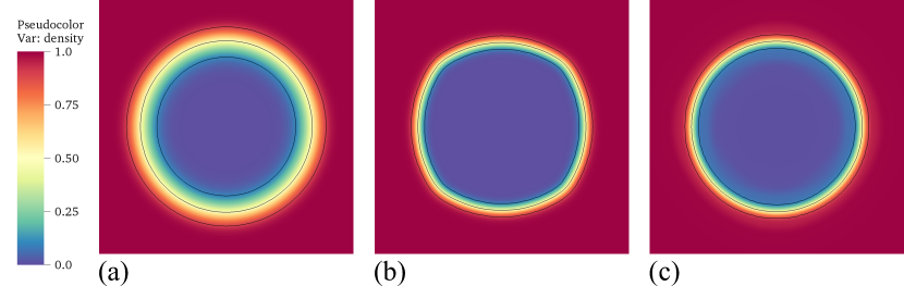
FIGURE 1: Comparison of the final state of the bubble after five flow-through times using (a) LAD approach, (b) divergence-form approach, and (c) gradient-form approach. The three solid black lines denote the isocontours of the volume fraction values of 0.1, 0.5, and 0.9, representing the interface region.

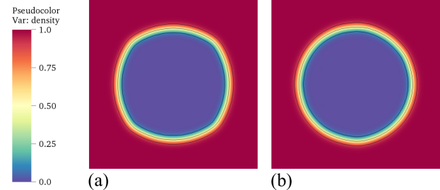
FIGURE 2: Comparison of the state of the bubble after five flow-through times using the divergence-form approach with (a) second-order scheme and (b) sixth-order scheme. The three solid black lines denote the isocontours of the volume fraction values of 0.1, 0.5, and 0.9, representing the interface region.

Two possible ways to mitigate the interface distortion are by refining the grid or by using a higher-order scheme for the interface-regularization terms. Because we are interested in the limit of coarse grid resolution, we study the effect of using an explicit sixth-order finite-difference scheme to discretize the interface regularization terms. As described in Section 2.8, finite-difference schemes may be used to discretize the interface regularization terms—without resulting in spurious behavior—if the nonlinear interface sharpening and the counteracting diffusion terms are formed at the grid faces (staggered locations), from which the derivatives at the grid points (nodes) may be calculated. Comparing the second-order and sixth-order schemes for the interface regularization terms of the divergence-form approach, the final state of the advecting bubble is shown in Figure 2. The interface distortion is significantly reduced using the sixth-order scheme.

Since the focus of the current work is on the evaluation of methods in a relatively coarser grid, we repeat the simulation of advection of an air bubble in water by scaling down the problem (in length and time) by a factor of $10$ without changing the number of grid points. The domain length is kept the same, but the new bubble radius is $2.5/89$, and the simulation is integrated for a total physical time of $t=0.1$ units. At this resolution, the bubble has $\approx 5$ grid points across its diameter, which represents a more realistic scenario that is encountered in large-scale engineering simulations.

The bubble at the final time is shown in Figure 3, for all the three methods. Similar to the more refined case above with the second-order finite-volume scheme, the divergence-form approach results in relatively faster shape distortion compared to the LAD method. Whereas, the gradient-form approach results in apparent complete loss of the bubble. Comparing this result with the refined simulation in Figure 1, this observation of mass loss on coarse grids is in good agreement with our hypothesis that the conservation error is proprotional to the local interface curvature and the under-resolved features are more prone to being lost due to the non-conservative nature of the method. This makes the gradient-form approach unsuitable for large-scale engineering simulations where it is only possible to afford a couple of grids points across a bubble/drop. To quantify the amount of mass loss with the gradient-form approach, the bubble mass is plotted against time for all three methods in Figure 4. Interestingly, around $40\%$ of the bubble mass is lost during the early time in the simulation and then the bubble mass saturates. This is due to the traces of mass of bubble that is still present in the domain, that is not under-resolved, after all the fine features are lost due to the conservation error.

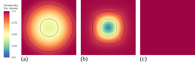
FIGURE 3: Comparison of the final state of the bubble on a coarse grid after five flow-through times using (a) LAD approach, (b) divergence-form approach, and (c) gradient-form approach. The two solid black lines denote the isocontours of the volume fraction values of 0.5 and 0.9, representing the interface region.

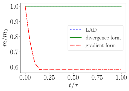
FIGURE 4: Plot of total mass, $m$, of the bubble by various methods, where $m_{0}$ is the mass at time $t=0$.

3.2 Shock interaction with a helium bubble in air

This section examines the classic test case of a shock wave traveling through air followed by an interaction with a stationary helium bubble. This case has been extensively studied using various numerical methods and models, such as a front-tracking method in Terashima and Tryggvason (2009); an arbitrary-Lagrangian Eulerian (ALE) method in Daude et al. (2014); anti-diffusion interface-capturing method in So et al. (2012); a ghost-fluid method (GFM) in Fedkiw et al. (1999), Bai and Deng (2017); a LAD diffuse-interface approach in Cook (2009); a gradient-form diffuse-interface approach in Shukla et al. (2010), and other diffuse-interface methods that implicitly capture the interface (no explicit interface-capturing method) using a WENO scheme in Johnsen and Colonius (2006), Coralic and Colonius (2014), using a TENO scheme in Haimovich and Frankel (2017), and using a WCNS scheme in Wong and Lele (2017). This test case has also been simulated with an adaptive-mesh-refinement technique in Quirk and Karni (1996) where a refined grid is used around the interface to improve the accuracy. More recently, this test case has also been studied in a three-dimensional setting in Deng et al. (2018).

To examine the interface regularization methods, we model this problem without physical species diffusion; therefore, the interface regularization methods for immiscible phases are applicable, because no physical molecular mixing should be exhibited by the underlying numerical model. The use of immiscible interface-capturing methods to model the interface between the gases in this problem is also motivated by the experiments of Haas and Sturtevant (1987). In these experiments, the authors use a thin plastic membrane to prevent molecular mixing of helium and air.

The problem domain spans $\left(-2\leq x\leq 4;\,0\leq y\leq 1\right)$, with periodic boundary conditions in the $y$ direction. A symmetry boundary is applied at $x=4$, representing a perfectly reflecting wall, and a sponge boundary condition is applied over $\left(-2\leq x\leq-1.5\right)$, modeling a non-reflecting free boundary. The problem is discretized on a uniform Cartesian grid of size $N_{x}=600$ and $N_{y}=100$. The bubble has a radius of $25/89$ and is initially placed at the location $(x=0,y=1/2)$. The material properties for the air medium are described by $\gamma_{1}=1.4$, $\rho_{1}=1.0$, ${p_{\infty}}_{1}=0$, $\mu_{1}=0$, and ${\sigma_{Y}}_{1}=0$. The material properties for the helium medium are described by $\gamma_{2}=1.67$, $\rho_{2}=0.138$, ${p_{\infty}}_{2}=0$, $\mu_{2}=0$, and ${\sigma_{Y}}_{2}=0$.

The initial conditions for the velocity, pressure, volume fraction, and density are

$$\begin{gathered}u=u^{(2)}f_{s}+u^{(1)}\left(1-f_{s}\right),\quad v=0,\quad p=p^{(2)}f_{s}+p^{(1)}\left(1-f_{s}\right),\\ \phi_{1}=\phi_{1}^{\epsilon}+\left(1-2\phi_{1}^{\epsilon}\right)f_{\phi},\quad\phi_{2}=1-\phi_{1},\quad\rho=\left(\phi_{1}\rho_{1}+\phi_{2}\rho_{2}\right)\left[\rho^{(2)}/\rho^{(1)}f_{s}+\left(1-f_{s}\right)\right],\end{gathered}$$ (46)

respectively, in which the volume fraction function, $f_{\phi}$, and the shock function, $f_{s}$, are given by

$$f_{\phi}=\frac{1}{2}\left\{1-\textrm{erf}\left[\frac{625/7921-x^{2}-\left(y-1/2\right)^{2}}{\Delta x}\right]\right\}\quad\textrm{and}\quad f_{s}=\frac{1}{2}\left[1-\textrm{erf}\left(\frac{x+1}{2\Delta x}\right)\right],$$ (47)

respectively, with jump conditions across the shock for velocity $\left(u^{(1)}=0;\,u^{(2)}=0.39473\right)$, density $\left(\rho^{(1)}=1\right.$, $\left.\rho^{(2)}=1.3764\right)$, and pressure $\left(p^{(1)}=1;\,p^{(2)}=1.5698\right)$. For this problem, the interface regularization length scale and the out-of-bounds velocity scale are defined by $\epsilon=\Delta x=0.01$ and $\Gamma^{*}=2.5$, respectively.

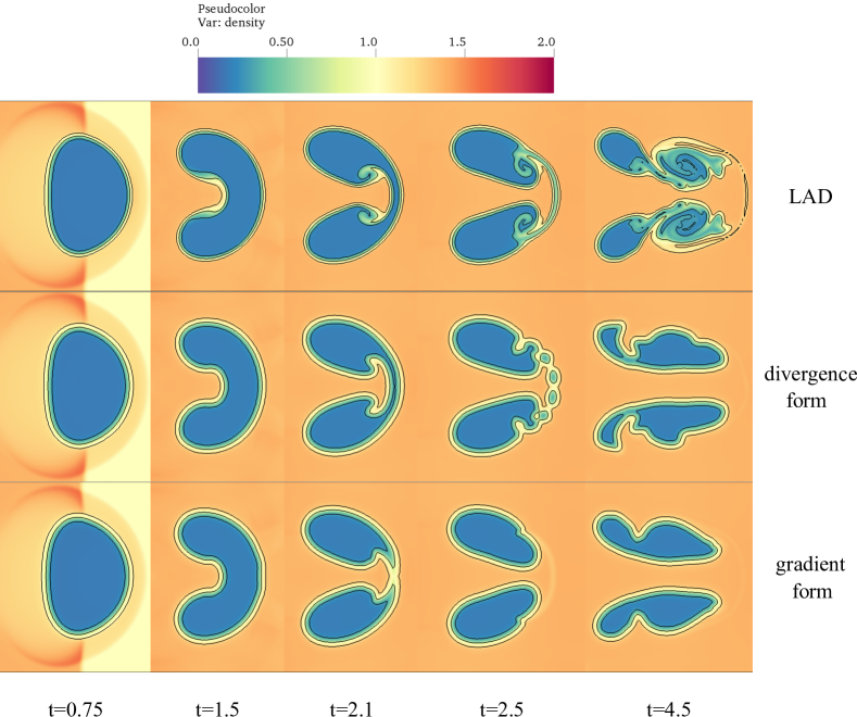
FIGURE 5: Comparison of the bubble shapes at different times for the case of the shock/helium-bubble-in-air interaction using various interface-capturing methods. The three solid black lines denote the isocontours of the volume fraction values of 0.1, 0.5, and 0.9, representing the interface region.

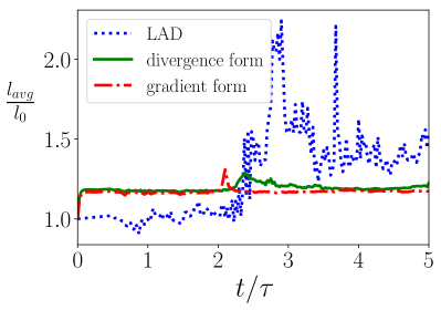
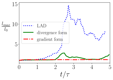
FIGURE 6: Comparison of the interface-thickness indicator, $l$, by various methods, where $l_{0}$ is the maximum interface thickness at time $t=0$. (a) Average interface thickness $l_{avg}$. (b) Maximum interface thickness $l_{max}$. To exclude unphysical spikes in $l_{max}$ during breakup events, a moving average of 5 local minima of $l_{max}$ is plotted.

The interaction of the shock with the helium bubble and the eventual breakup of the bubble are shown in Figure 5, with depictions of the evolution at various times, for LAD, divergence-form, and gradient-form approaches. The bubble can be seen to undergo breakup at an approximate (non-dimensional) time of $t=2.5$. After this time, the simulation cannot be considered physical because of the under-resolved processes associated with the breakup and the lack of explicit subgrid models for these processes; each interface regularization approach treats the under-resolved processes differently. Therefore, there is no consensus on the final shape of the bubble among the three methods. Yet, a qualitative comparison between the three methods can still be made using the results presented in Figure 5.

Using the LAD approach, the interface diffuses excessively in the regions of high shear, unlike the divergence-form and gradient-form approaches, where the interface thickness is constant throughout the simulation. However, using the LAD approach, the interface remains sharp in the regions where there is no shearing. To quantify the amount of interface diffusion, the interface-thickness indicator [$l$ of Eq. (43)] is plotted in Figure 6 for the three methods. The average thickness, $l_{avg}$, increases slightly for the LAD method around $t/\tau\approx 2$, but the maximum interface thickness, $l_{max}$, increases almost $15$ times for the LAD method, whereas it remains on the order of one for the other two methods. This demonstrates a deficiency of the LAD approach for problems that involve significant shearing at an interface that is not subjected to compression.

Furthermore, the behavior of bubble breakup is significantly different among the various methods. Depending on the application, any one of these methods may or may not result in an appropriate representation of the under-resolved processes. However, for the current study that involves modeling interfaces between immiscible fluids, the grid-induced breakup of the divergence-form approach may be more suitable than the diffusion of the fine structures in the LAD approach or the premature loss of fine structures and associated conservation error of the gradient-form approach. For the LAD approach, the thin film formed at around time $t=2.1$ does not break; rather, it evolves into a thin region of well-mixed fluid. This behavior may be considered unphysical for two immiscible fluids, for which the physical interface is infinitely sharp in a continuum sense; this behavior would be more appropriate for miscible fluids. For the divergence-form approach, the thin film forms satellite bubbles, which is expected when there is a breakage of a thin ligament between droplets or bubbles due to surface-tension effects. However, this breakup may not be considered completely physical without any surface-tension forces, because the breakup is triggered by the lack of grid support. For the gradient-form approach, the thin film formed at around time $t=2.1$ breaks prematurely and disappears with no formation of satellite bubbles, and the mass of the film is lost to conservation error.

In Figure 2 of Shukla et al. (2010), without the use of interface regularization terms, the interface thickness is seen to increase significantly. Their approach without interface regularization terms is most similar to our LAD approach, because the LAD approach does not include any sharpening terms. Therefore, comparing these results suggests that the thickening of the interface in their case was due to the use of the more dissipative Riemann-solver/reconstruction scheme. The results from the gradient-form approach also match well with the results of the similar method shown in Figure 2 of Shukla et al. (2010), which further verifies our implementation. Finally, there is no consensus on the final shape of the bubble among the three methods, which is to be expected, because there are no surface-tension forces and the breakup is triggered by the lack of grid resolution.

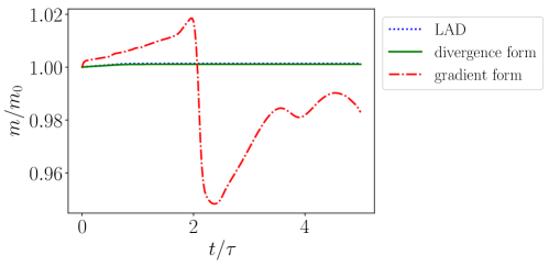
FIGURE 7: Plot of total mass, $m$, of the helium bubble by various methods, where $m_{0}$ is the mass at time $t=0$.

To further quantify the amount of mass lost or gained, the total mass of the bubble is computed using Eq. (41) and is plotted over time in Figure 7. The mass of the bubble is conserved for the LAD and divergence-form approaches, but is not conserved for the gradient-form approach, as expected. The loss of mass is observed to be largest when the bubble is about to break, for the gradient form approach. This is because the mass-conservation error in the gradient-form approach is proportional to the local curvature, as described in Section 2.7. Therefore, at the onset of breakup, thin film rupture is different from the other two methods, and the satellite bubbles are absent.

3.3 Shock interaction with an air bubble in water

This section examines a shock wave traveling through water followed by an interaction with a stationary air bubble. The material properties are the same as those described in Section 3.1. This test case is based on the experiments in Bourne and Field (1992) and has been widely used as a validation case for various numerical methods and models such as a front-tracking method in Terashima and Tryggvason (2009); a level-set method in Hu and Khoo (2004), Nourgaliev et al. (2006); a ghost-fluid method in Bai and Deng (2017); a volume-of-fluid method in Bo and Grove (2014); an implicit diffuse-interface method with a Godunov scheme in Ansari and Daramizadeh (2013), and with a TENO scheme in Haimovich and Frankel (2017); and with a gradient-form diffuse-interface approach in Shukla et al. (2010), Shukla (2014).

The initial conditions for the velocity, pressure, volume fraction, and density are

$$\begin{gathered}u=u^{(2)}f_{s}+u^{(1)}\left(1-f_{s}\right),\quad v=0,\quad p=p^{(2)}f_{s}+p^{(1)}\left(1-f_{s}\right),\\ \phi_{1}=\phi_{1}^{\epsilon}+\left(1-2\phi_{1}^{\epsilon}\right)f_{\phi},\quad\phi_{2}=1-\phi_{1},\quad\rho=\left(\phi_{1}\rho_{1}+\phi_{2}\rho_{2}\right)\left[\rho^{(2)}/\rho^{(1)}f_{s}+\left(1-f_{s}\right)\right],\\ \end{gathered}$$ (48)

respectively, in which the volume fraction function, $f_{\phi}$, and the shock function, $f_{s}$, are given by,

$$f_{\phi}=\frac{1}{2}\left\{1-\textrm{erf}\left[\frac{1-\left(x-2.375\right)^{2}-\left(y-2.5\right)^{2}}{\Delta x}\right]\right\}\quad\textrm{and}\quad f_{s}=\frac{1}{2}\left[1-\textrm{erf}\left(\frac{x+1}{10\Delta x}\right)\right],$$ (49)

respectively, with jump conditions across the shock for velocity $\left(u^{(1)}=0;\,u^{(2)}=68.5176\right)$, density $\left(\rho^{(1)}=1\right.$, $\left.\rho^{(2)}=1.32479\right)$, and pressure $\left(p^{(1)}=1;\,p^{(2)}=19150\right)$. The problem domain spans $\left(-2\leq x\leq 8;\,0\leq y\leq 5\right)$, with periodic boundary conditions in the $y$ direction. A symmetry boundary is applied at $x=8$, representing a perfectly reflecting wall, and a sponge boundary condition is applied over $\left(-2\leq x\leq-1.5\right)$, modeling a non-reflecting free boundary. The problem is discretized on a uniform Cartesian grid of size $N_{x}=400$ and $N_{y}=200$.

For this problem, the artificial bulk viscosity, artificial thermal conductivity, artificial diffusivity, interface regularization length scale, interface regularization velocity scale, and out-of-bounds velocity scale are defined by $C_{\beta}=20$, $C_{\kappa}=0.1$, $C_{D}=20$, $\epsilon=\Delta x=2.5\times 10^{-2}$, $\Gamma=2.0$, and $\Gamma^{*}=0.0$, respectively. A fourth-order, penta-diagonal, Padé filter is employed for dealiasing in this problem to improve the stability of the shock/bubble interaction. The linear system defining this filter is given by

$$\hat{f}_{i}+\alpha(\hat{f}_{i+1}+\hat{f}_{i-1})+\frac{1-2\alpha}{14}(\hat{f}_{i+2}+\hat{f}_{i-2})=\frac{4+6\alpha}{7}f_{i}+\frac{2+3\alpha}{7}(f_{i+1}+f_{i-1})$$ (50)

where $\alpha=0.499$.

Notably, for this problem, the LAD in the mass equations is also necessarily included in the divergence-form and gradient-form approaches to maintain stability. The latter approaches become unstable for this problem for large $\Gamma$ (the velocity scale for interface regularization). Figure 8 describes the evolution in time of the shock/bubble interaction and the subsequent bubble collapse. There is no significant difference between the various regularization methods for this problem. The similarity is due to the short convective timescale of the flow relative to the maximum stable timescale of the volume fraction regularization methods; effectively, all methods remain qualitatively similar to the LAD approach.

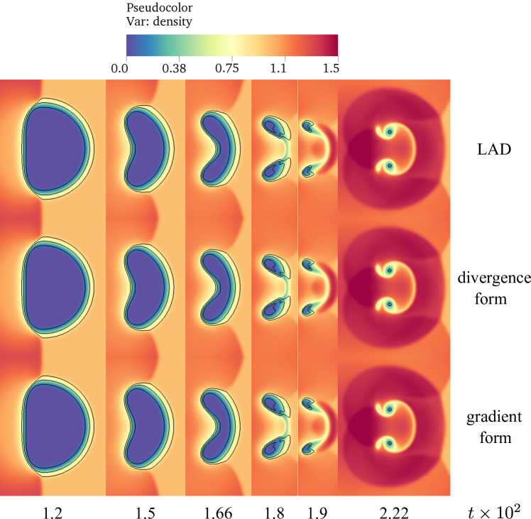
FIGURE 8: Comparison of the bubble shapes at different times for the case of shock/air-bubble-in-water interaction using various interface-capturing methods. The three solid black lines denote the isocontours of the volume fraction values of 0.1, 0.5, and 0.9, representing the interface region.

3.4 Richtmyer–Meshkov instability of a copper–aluminum interface

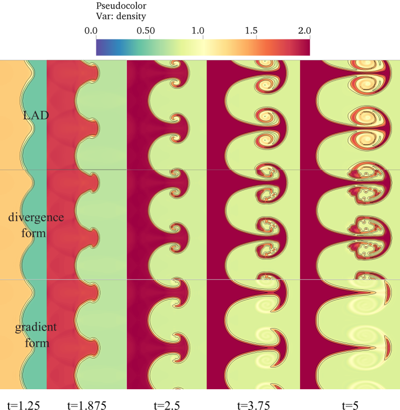
FIGURE 9: Comparison of the copper–aluminum interface shapes at different times for the Cu-Al RMI case using various interface-capturing methods. The three solid black lines denote the isocontours of the volume fraction values of 0.1, 0.5, and 0.9, representing the interface region.

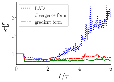
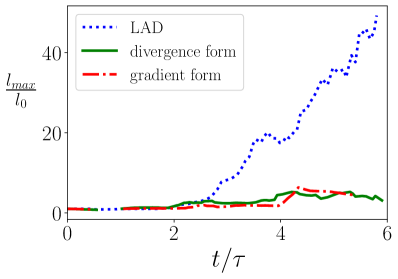
FIGURE 10: Comparison of the interface-thickness indicator, $l$, by various methods, where $l_{0}$ is the maximum interface thickness at time $t=0$. (a) Average interface thickness $l_{avg}$. (b) Maximum interface thickness $l_{max}$. To exclude unphysical spikes in $l_{max}$ during breakup events, a moving average of 5 local minima of $l_{max}$ is plotted.

This section examines a shock wave traveling through copper followed by an interaction with a sinusoidally distorted copper–aluminum material interface. Though this problem has not been as widely studied as the previous examples, it is included to demonstrate how interface regularization methods perform when extended to problems involving elastic-plastic deformation at material interfaces. Such deformation may arise in impact welding, where interfacial instabilities are known to develop as metal plates impact and shear (Nassiri et al., 2016); as well as material characterization at high strain rates, which typically employ a metal-gas configuration of the Richtmyer-Meshkov instability (Dimonte et al., 2011). The copper-aluminum variant of this problem was previously studied by Lopez Ortega (2013), who used a level-set method combined with the modified ghost-fluid method to set boundary conditions at material interfaces. This problem was also studied by Subramaniam et al. (2018) and Adler and Lele (2019), and the results presented here are an extension of that work.

The problem domain spans $\left(-2\leq x\leq 4;\,0\leq y\leq 1\right)$, with periodic boundary conditions in the $y$ direction. A symmetry boundary is applied at $x=4$, representing a perfectly reflecting wall, and a sponge boundary condition is applied over $\left(-2\leq x\leq-1.5\right)$, modeling a non-reflecting free boundary. The problem is discretized on a uniform Cartesian grid of size $N_{x}=768$ and $N_{y}=128$. The material properties for the copper medium are described by $\gamma_{1}=2.0$, $\rho_{1}=1.0$, ${p_{\infty}}_{1}=1.0$, $\mu_{1}=0.2886$, and ${\sigma_{Y}}_{1}=8.79\times 10^{-4}$. The material properties for the aluminum medium are described by $\gamma_{2}=2.088$, $\rho_{2}=0.3037$, ${p_{\infty}}_{2}=0.5047$, $\mu_{2}=0.1985$, and ${\sigma_{Y}}_{2}=2.176\times 10^{-3}$.

The initial conditions for the velocity, pressure, volume fraction, and density are

$$\begin{gathered}u=u^{(2)}f_{s}+u^{(1)}\left(1-f_{s}\right),\quad v=0,\quad p=p^{(2)}f_{s}+p^{(1)}\left(1-f_{s}\right),\\ \phi_{1}=\phi_{1}^{\epsilon}+\left(1-2\phi_{1}^{\epsilon}\right)f_{\phi},\quad\phi_{2}=1-\phi_{1},\quad\rho=\left(\phi_{1}\rho_{1}+\phi_{2}\rho_{2}\right)\left[\rho^{(2)}/\rho^{(1)}f_{s}+\left(1-f_{s}\right)\right],\end{gathered}$$ (51)

respectively, in which the volume fraction function, $f_{\phi}$, and the shock function, $f_{s}$, are given by

$$f_{\phi}=\frac{1}{2}\left(1-\textrm{erf}\left\{\frac{x-\left[2+0.4/\left(4\pi y\right)\sin\left(4\pi y\right)\right]}{3\Delta x}\right\}\right)\quad\textrm{and}\quad f_{s}=\frac{1}{2}\left[1-\textrm{erf}\left(\frac{x-1}{2\Delta x}\right)\right],$$ (52)

respectively, with jump conditions across the shock for velocity $\left(u^{(1)}=0;\,u^{(2)}=0.68068\right)$, density $\left(\rho^{(1)}=1\right.$, $\left.\rho^{(2)}=1.4365\right)$, and pressure $\left(p^{(1)}=5\times 10^{-2};\,p^{(2)}=1.25\right)$. The kinematic tensors are initialized in a pre-strained state consistent with the material compression associated with shock initialization, assuming no plastic deformation has yet occurred, with

$$g_{ij}=g^{e}_{ij}=\begin{cases}\left[\rho^{(2)}f_{s}+\rho^{(1)}\left(1-f_{s}\right)\right]/\rho_{1},&\text{for }i=j=1\\ \delta_{ij},&\text{else }\end{cases}\qquad\textrm{and}\qquad g^{p}_{ij}=\delta_{ij}.$$ (53)

For this problem, the interface regularization length scale and the out-of-bounds velocity scale for the divergence form method are defined by $\epsilon=\Delta x/2=3.90625\times 10^{-3}$ and $\Gamma^{*}=1.0$, respectively. For the gradient form method, it is necessary for stability to use $\epsilon=3\Delta x/4=5.859375\times 10^{-3}$, $\Gamma^{*}=1.0$, and $\phi_{min}=1\times 10^{-5}$.

The time evolution of the growth of the interface instability is shown in Figure 9. The simulation is integrated well into the nonlinear regime where the bubble (lighter medium) and the spike (heavier medium) have interpenetrated, forming mushroom-shaped structures with fine ligaments. The qualitative comparison between the methods in this test case is similar to that of the shock-helium-bubble interaction in air. With the LAD approach, the interface thickness increases with time, especially in the regions of high shear at the later stages. However, with the divergence-form and gradient-form approaches, the interface thickness is constant throughout the simulation. This is quantified by plotting the interface-thickness indicator [$l$ of Eq. (43)] for each of the three methods in Figure 10. The average thickness, shown in Figure 10(a) shows a sharp drop in thickness at $t/\tau\approx 0.5$ when the shock passes through the interface. After this, the thickness remains small for both the gradient and divergence form methods, whereas with LAD the interface thickness grows gradually after $t/\tau\approx 2$, when the interface begins to roll up. Figure 10(b) shows the maximum interface thickness, which increases almost $60$ times for the LAD method, whereas it stays on the order of one for the other two methods. This illustrates that the LAD method incurs significant artificial diffusion when the interface deformation cannot be resolved by the grid.

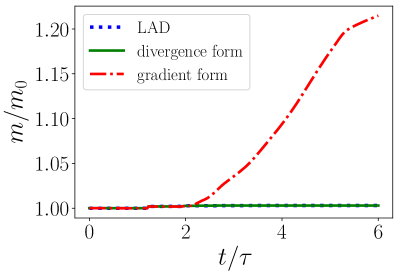
FIGURE 11: Plot of total mass, $m$, of aluminum by various methods, where $m_{0}$ is the mass at time $t=0$.

It is also evident from Figure 9 that the gradient-form approach results in significant copper mass loss, and the dominant mushroom structure formed in the nonlinear regime is completely lost. To quantify the amount of mass lost or gained, the total mass of the aluminum material [Eq. (41)] is plotted against time in Figure 11. The gradient-form approach results in significant gain in the mass of the aluminum material, up to $20\%$, as the grid can no longer resolve the increased interface curvature during roll-up. This makes it practically unsuitable for accurate interface representation for long-time numerical simulations. With the divergence-form approach, the breakage of the ligaments to form metallic droplets can be seen in Figure 9.

4 Summary and concluding remarks

This work examines three diffuse-interface-capturing methods and evaluates their performance for the simulation of immiscible compressible multiphase fluid flows and elastic-plastic deformation in solids. The first approach is the localized-artificial-diffusivity method of Cook (2007), Subramaniam et al. (2018), and Adler and Lele (2019), in which artificial diffusion terms are added to the individual phase mass fraction transport equations and are coupled with the other conservation equations. The second approach is the gradient-form approach that is based on the quasi-conservative method of Shukla et al. (2010). In this method, the diffusion and sharpening terms (together called regularization terms) are added to the individual phase volume fraction transport equations and are coupled with the other conservation equations (Tiwari et al., 2013). The third approach is the divergence-form approach that is based on the fully conservative method of Jain et al. (2020). In this method, the diffusion and sharpening terms are added to the individual phase volume fraction transport equations and are coupled with the other conservation equations. In the present study, all of these interface regularization methods are used in conjunction with a four-equation, multicomponent mixture model, in which pressure and temperature equilibria are assumed among the various phases. The latter two interface regularization methods are commonly used in the context of a five-equation model, in which temperature equilibrium is not assumed.

The primary objective of this work is to compare these three methods in terms of their ability to: maintain constant interface thickness throughout the simulation; conserve mass of each of the phases, mixture momentum, and total energy; and maintain accurate interface shape for long-time integration. The secondary objective of this work is to extend these methods for modeling the interface between deforming solid materials with strength. The LAD method has previously been used for simulating material interfaces between solids with strength (Subramaniam et al., 2018, Adler and Lele, 2019). Here, we introduce consistent corrections in the kinematic equations for the divergence-form and the gradient-form approaches to extend these methods for the simulation of interfaces between solids with strength.

Method Conservation Sharp interface Shape preservation Behavior of under-resolved ligaments and breakup LAD Yes No (interface diffuses in the regions of high shear) Yes Artificial diffusion (fine-scale features artificially diffuse as they approach unresolved scales) Divergence form Yes Yes No (interface aligns with the grid) Artificial breakup (fine-scale features artificially break up as they approach unresolved scales) Gradient form No (under-resolved features will be lost) Yes Yes Artificial loss of mass (fine-scale features are lost, due to conservation error, as they approach unresolved scales)

TABLE 1: Summary of the advantages and disadvantages of the three diffuse-interface capturing methods considered in this study: LAD method based on Cook (2007), Subramaniam et al. (2018), and Adler and Lele (2019); divergence-form approach based on Jain et al. (2020); and the gradient-form approach based on Shukla et al. (2010) and Tiwari et al. (2013). The relative disadvantages of each approach and the different behaviors of under-resolved processes are underlined.

We employ several test cases to evaluate the performance of the methods, including (1) advection of an air bubble in water, (2) shock interaction with a helium bubble in air, (3) shock interaction and the collapse of an air bubble in water, and (4) Richtmyer–Meshkov instability of a copper–aluminum interface. For the application of these methods to large-scale simulations of engineering interest, it is rarely practical to use hundreds of grid points to resolve the diameter of a bubble/drop. Therefore, we choose to study the limit of relatively coarse grid resolution, which is more representative of the true performance of these methods.

The performance of the three methods is summarized in Table 1. The LAD and the divergence-form approaches conserve mass, momentum, and energy, whereas the gradient-form approach does not. The mass-conservation error increases proportionately with the local interface curvature; therefore, fine interfacial structures will be lost during the simulation. The divergence-form and the gradient-form approaches maintain a constant interface thickness throughout the simulation, whereas the interface thickness of the LAD method increases in the regions of high shear due to the lack of interface sharpening terms to counter the artificial diffusion. The LAD and the gradient-form approaches maintain the interface shape for a long time compared to the divergence-form approach; however, the interface distortion of the divergence-form approach can be mitigated with the use of appropriately crafted higher-order schemes for the interface regularization terms.

For each method, the behavior of under-resolved ligaments and breakup features is unique. For the LAD approach, thin ligaments that form at the onset of bubble breakup (or in late-stage RMI) diffuse instead of rupturing. For the gradient-form approach, the ligament formation is not captured because of mass-conservation issues, which result in premature loss of these fine-scale features. For the divergence-form approach, the ligaments rupture due to the lack of grid support, acting like an artificial surface tension force that becomes significant at the grid scale.

For broader applications, the optimal method depends on the objectives of the study. These applications include (1) well-resolved problems, in which differences in the behavior of under-resolved features is not of concern, (2) applications involving interfaces between miscible phases, and (3) applications involving more complex physics, including regimes in which surface tension or molecular diffusion must be explicitly modeled and problems in which phase changes occur. We intend this demonstration of the advantages, disadvantages, and behavior of under-resolved phenomena exhibited by the various methods to be helpful, albeit being unphysical, in the selection of an interface-regularization method. These results also provide motivation for the development of subgrid models for multiphase flows.

Appendix A: Finite-difference operators for the divergence-form approach

The test case of shock interaction with a helium bubble in air is repeated for the divergence-form approach with the same parameters listed in Section 3.2. Here, the difference is in the numerical representation of the nonlinear interface-regularization terms. In Section 3.2, the interface-regularization fluxes are formed at the faces, as described in Section 2.8, which is consistent with the finite-volume implementation in Jain et al. (2020). Whereas, here, a second-order standard central finite-difference scheme is used instead.

The shock interaction with the helium bubble in air and the subsequent evolution of the bubble shape are shown in Figure 12. An unphysical wrinkling of the interface can be seen at the later stages of the bubble deformation. This behavior is consistent with the observations made by Shukla et al. (2010), which motivated them to develop the gradient-form approach. However, discretizing the fluxes at the faces, Jain et al. (2020) showed that this results in discrete balance between the diffusion and sharpening fluxes, thereby eliminating the spurious wrinkling of the interface as can be seen in Figure 5. In this work, this face-evaluated flux formulation has been succesfully extended for higher-order schemes and is presented in Section 2.8.

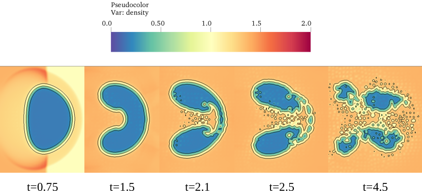
FIGURE 12: The bubble shapes at different times for the case of the shock/helium-bubble-in-air interaction using the divergence-form approach, where the interface-regularization terms are discretized using a second-order standard central finite-difference scheme. The three solid black lines denote the isocontours of the volume fraction values of 0.1, 0.5, and 0.9, representing the interface region.

References

- Cook (2007) A. W. Cook, Artificial fluid properties for large-eddy simulation of compressible turbulent mixing, Physics of fluids 19 (2007) 055103.
- Subramaniam et al. (2018) A. Subramaniam, N. S. Ghaisas, S. K. Lele, High-order Eulerian simulations of multimaterial elastic–plastic flow, Journal of Fluids Engineering 140 (2018) 050904.
- Adler and Lele (2019) M. C. Adler, S. K. Lele, Strain-hardening framework for Eulerian simulations of multi-material elasto-plastic deformation, in: Center for Turbulence Research Annual Research Briefs 2019, Stanford University, 2019.
- Shukla et al. (2010) R. K. Shukla, C. Pantano, J. B. Freund, An interface capturing method for the simulation of multi-phase compressible flows, Journal of Computational Physics 229 (2010) 7411–7439.
- Tiwari et al. (2013) A. Tiwari, J. B. Freund, C. Pantano, A diffuse interface model with immiscibility preservation, Journal of Computational Physics 252 (2013) 290–309.
- Jain et al. (2020) S. S. Jain, A. Mani, P. Moin, A conservative diffuse-interface method for compressible two-phase flows, Journal of Computational Physics (2020) 109606.
- Kataoka (1986) I. Kataoka, Local instant formulation of two-phase flow, International Journal of Multiphase Flow 12 (1986) 745–758.
- Shyue (1998) K.-M. Shyue, An efficient shock-capturing algorithm for compressible multicomponent problems, Journal of Computational Physics 142 (1998) 208–242.
- Venkateswaran et al. (2002) S. Venkateswaran, J. W. Lindau, R. F. Kunz, C. L. Merkle, Computation of multiphase mixture flows with compressibility effects, Journal of Computational Physics 180 (2002) 54–77.
- Marquina and Mulet (2003) A. Marquina, P. Mulet, A flux-split algorithm applied to conservative models for multicomponent compressible flows, Journal of Computational Physics 185 (2003) 120–138.
- Cook (2009) A. W. Cook, Enthalpy diffusion in multicomponent flows, Physics of Fluids 21 (2009) 055109.
- Allaire et al. (2002) G. Allaire, S. Clerc, S. Kokh, A five-equation model for the simulation of interfaces between compressible fluids, Journal of Computational Physics 181 (2002) 577–616.
- Kapila et al. (2001) A. K. Kapila, R. Menikoff, J. B. Bdzil, S. F. Son, D. S. Stewart, Two-phase modeling of deflagration-to-detonation transition in granular materials: Reduced equations, Physics of Fluids 13 (2001) 3002–3024.
- So et al. (2012) K. So, X. Hu, N. Adams, Anti-diffusion interface sharpening technique for two-phase compressible flow simulations, Journal of Computational Physics 231 (2012) 4304–4323.
- Ansari and Daramizadeh (2013) M. Ansari, A. Daramizadeh, Numerical simulation of compressible two-phase flow using a diffuse interface method, International Journal of Heat and Fluid Flow 42 (2013) 209–223.
- Shukla (2014) R. K. Shukla, Nonlinear preconditioning for efficient and accurate interface capturing in simulation of multicomponent compressible flows, Journal of Computational Physics 276 (2014) 508–540.
- Coralic and Colonius (2014) V. Coralic, T. Colonius, Finite-volume WENO scheme for viscous compressible multicomponent flows, Journal of Computational Physics 274 (2014) 95–121.
- Perigaud and Saurel (2005) G. Perigaud, R. Saurel, A compressible flow model with capillary effects, Journal of Computational Physics 209 (2005) 139–178.
- Wong and Lele (2017) M. L. Wong, S. K. Lele, High-order localized dissipation weighted compact nonlinear scheme for shock-and interface-capturing in compressible flows, Journal of Computational Physics 339 (2017) 179–209.
- Chiapolino et al. (2017) A. Chiapolino, R. Saurel, B. Nkonga, Sharpening diffuse interfaces with compressible fluids on unstructured meshes, Journal of Computational Physics 340 (2017) 389–417.
- Garrick et al. (2017a) D. P. Garrick, W. A. Hagen, J. D. Regele, An interface capturing scheme for modeling atomization in compressible flows, Journal of Computational Physics 344 (2017a) 260–280.
- Garrick et al. (2017b) D. P. Garrick, M. Owkes, J. D. Regele, A finite-volume HLLC-based scheme for compressible interfacial flows with surface tension, Journal of Computational Physics 339 (2017b) 46–67.
- Jain et al. (2018) S. S. Jain, A. Mani, P. Moin, A conservative diffuse-interface method for the simulation of compressible two-phase flows with turbulence and acoustics, Center for Turbulence Research Annual Research Briefs (2018) 47–64.
- Yeom and Chang (2013) G.-S. Yeom, K.-S. Chang, A modified HLLC-type Riemann solver for the compressible six-equation two-fluid model, Computers & Fluids 76 (2013) 86–104.
- Baer and Nunziato (1986) M. Baer, J. Nunziato, A two-phase mixture theory for the deflagration-to-detonation transition (ddt) in reactive granular materials, International journal of multiphase flow 12 (1986) 861–889.
- Sainsaulieu (1995) L. Sainsaulieu, Finite volume approximation of two phase-fluid flows based on an approximate Roe-type Riemann solver, Journal of Computational Physics 121 (1995) 1–28.
- Saurel and Abgrall (1999) R. Saurel, R. Abgrall, A simple method for compressible multifluid flows, SIAM Journal on Scientific Computing 21 (1999) 1115–1145.
- Mirjalili et al. (2017) S. Mirjalili, S. S. Jain, M. Dodd, Interface-capturing methods for two-phase flows: An overview and recent developments, Center for Turbulence Research Annual Research Briefs (2017) 117–135.
- Saurel and Pantano (2018) R. Saurel, C. Pantano, Diffuse-interface capturing methods for compressible two-phase flows, Annual Review of Fluid Mechanics 50 (2018).
- Aslani and Regele (2018) M. Aslani, J. D. Regele, A localized artificial diffusivity method to simulate compressible multiphase flows using the stiffened gas equation of state, International Journal for Numerical Methods in Fluids 88 (2018) 413–433.
- Francois et al. (2006) M. M. Francois, S. J. Cummins, E. D. Dendy, D. B. Kothe, J. M. Sicilian, M. W. Williams, A balanced-force algorithm for continuous and sharp interfacial surface tension models within a volume tracking framework, Journal of Computational Physics 213 (2006) 141–173.
- Mencinger and Žun (2007) J. Mencinger, I. Žun, On the finite volume discretization of discontinuous body force field on collocated grid: Application to VOF method, Journal of Computational Physics 221 (2007) 524–538.
- Jain and Moin (2020) S. S. Jain, P. Moin, A kinetic energy and entropy preserving scheme for the simulation of compressible two-phase turbulent flows, Center for Turbulence Research Annual Research Briefs (2020).
- Benson (1992) D. J. Benson, Computational methods in Lagrangian and Eulerian hydrocodes, Computer Methods in Applied Mechanics and Engineering 99 (1992) 235–394.
- Donea et al. (2004) J. Donea, A. Huerta, J.-P. Ponthot, A. Rodríguez-Ferran, Arbitrary Lagrangian–Eulerian methods, Encyclopedia of Computational Mechanics 1 (2004) 413–437. Chapter 14.
- Miller and Colella (2001) G. H. Miller, P. Colella, A high-order Eulerian Godunov method for elastic–plastic flow in solids, Journal of Computational Physics 167 (2001) 131–176.
- Ortega et al. (2014) A. L. Ortega, M. Lombardini, D. Pullin, D. I. Meiron, Numerical simulation of elastic–plastic solid mechanics using an Eulerian stretch tensor approach and HLLD Riemann solver, Journal of Computational Physics 257 (2014) 414–441.
- Ghaisas et al. (2018) N. S. Ghaisas, A. Subramaniam, S. K. Lele, A unified high-order Eulerian method for continuum simulations of fluid flow and of elastic–plastic deformations in solids, Journal of Computational Physics 371 (2018) 452–482.
- Sugiyama et al. (2010) K. Sugiyama, S. Ii, S. Takeuchi, S. Takagi, Y. Matsumoto, Full Eulerian simulations of biconcave neo-Hookean particles in a Poiseuille flow, Computational Mechanics 46 (2010) 147–157.
- Sugiyama et al. (2011) K. Sugiyama, S. Ii, S. Takeuchi, S. Takagi, Y. Matsumoto, A full Eulerian finite difference approach for solving fluid–structure coupling problems, Journal of Computational Physics 230 (2011) 596–627.
- Favrie and Gavrilyuk (2011) N. Favrie, S. Gavrilyuk, Mathematical and numerical model for nonlinear viscoplasticity, Philosophical Transactions of the Royal Society A: Mathematical, Physical and Engineering Sciences 369 (2011) 2864–2880.
- Valkov et al. (2015) B. Valkov, C. H. Rycroft, K. Kamrin, Eulerian method for multiphase interactions of soft solid bodies in fluids, Journal of Applied Mechanics 82 (2015).
- Jain et al. (2019) S. S. Jain, K. Kamrin, A. Mani, A conservative and non-dissipative eulerian formulation for the simulation of soft solids in fluids, Journal of Computational Physics 399 (2019) 108922.
- Ghaisas et al. (2017) N. S. Ghaisas, A. Subramaniam, S. K. Lele, A. W. Cook, Evaluation of an Eulerian multi-material mixture formulation based on a single inverse deformation gradient tensor field, Center for Turbulence Research Annual Briefs 2017 (2017).
- Plohr and Sharp (1992) B. J. Plohr, D. H. Sharp, A conservative formulation for plasticity, Advances in Applied Mathematics 13 (1992) 462–493.
- Adler et al. (2021) M. C. Adler, J. R. West, S. K. Lele, A high-order method for eulerian simulation of multi-material elasto-plastic deformation with strain hardening (in preparation), 2021.
- Ndanou et al. (2015) S. Ndanou, N. Favrie, S. Gavrilyuk, Multi-solid and multi-fluid diffuse interface model: Applications to dynamic fracture and fragmentation, Journal of Computational Physics 295 (2015) 523–555.
- Ortega et al. (2015) A. L. Ortega, M. Lombardini, P. T. Barton, D. I. Pullin, D. I. Meiron, Richtmyer–Meshkov instability for elastic–plastic solids in converging geometries, Journal of the Mechanics and Physics of Solids 76 (2015) 291–324.
- Lele (1992) S. K. Lele, Compact finite difference schemes with spectral-like resolution, Journal of Computational Physics 103 (1992) 16–42.
- Ghate et al. (2021) A. S. Ghate, A. Subramaniam, N. Ghaisas, J. R. West, M. C. Adler, S. S. Jain, PadéOps source code, 2021. DOI: 10.5281/zenodo.5277989.
- Chiodi and Desjardins (2017) R. Chiodi, O. Desjardins, A reformulation of the conservative level set reinitialization equation for accurate and robust simulation of complex multiphase flows, Journal of Computational Physics 343 (2017) 186–200.
- Murrone and Guillard (2005) A. Murrone, H. Guillard, A five equation reduced model for compressible two phase flow problems, Journal of Computational Physics 202 (2005) 664–698.
- Johnsen and Ham (2012) E. Johnsen, F. Ham, Preventing numerical errors generated by interface-capturing schemes in compressible multi-material flows, Journal of Computational Physics 231 (2012) 5705–5717.
- Saurel et al. (2009) R. Saurel, F. Petitpas, R. A. Berry, Simple and efficient relaxation methods for interfaces separating compressible fluids, cavitating flows and shocks in multiphase mixtures, journal of Computational Physics 228 (2009) 1678–1712.
- Johnsen and Colonius (2006) E. Johnsen, T. Colonius, Implementation of WENO schemes in compressible multicomponent flow problems, Journal of Computational Physics 219 (2006) 715–732.
- Beig and Johnsen (2015) S. A. Beig, E. Johnsen, Maintaining interface equilibrium conditions in compressible multiphase flows using interface capturing, Journal of Computational Physics 302 (2015) 548–566.
- Capuano et al. (2018) M. Capuano, C. Bogey, P. D. Spelt, Simulations of viscous and compressible gas–gas flows using high-order finite difference schemes, Journal of Computational Physics 361 (2018) 56–81.
- Shyue and Xiao (2014) K.-M. Shyue, F. Xiao, An eulerian interface sharpening algorithm for compressible two-phase flow: The algebraic thinc approach, Journal of Computational Physics 268 (2014) 326–354.
- Haimovich and Frankel (2017) O. Haimovich, S. H. Frankel, Numerical simulations of compressible multicomponent and multiphase flow using a high-order targeted eno (teno) finite-volume method, Computers & Fluids 146 (2017) 105–116.
- Terashima and Tryggvason (2009) H. Terashima, G. Tryggvason, A front-tracking/ghost-fluid method for fluid interfaces in compressible flows, Journal of Computational Physics 228 (2009) 4012–4037.
- Daude et al. (2014) F. Daude, P. Galon, Z. Gao, E. Blaud, Numerical experiments using a hllc-type scheme with ale formulation for compressible two-phase flows five-equation models with phase transition, Computers & Fluids 94 (2014) 112–138.
- Fedkiw et al. (1999) R. P. Fedkiw, T. Aslam, B. Merriman, S. Osher, et al., A non-oscillatory eulerian approach to interfaces in multimaterial flows (the ghost fluid method), Journal of computational physics 152 (1999) 457–492.
- Bai and Deng (2017) X. Bai, X. Deng, A sharp interface method for compressible multi-phase flows based on the cut cell and ghost fluid methods, Advances in Applied Mathematics and Mechanics 9 (2017) 1052–1075.
- Quirk and Karni (1996) J. J. Quirk, S. Karni, On the dynamics of a shock–bubble interaction, Journal of Fluid Mechanics 318 (1996) 129–163.
- Deng et al. (2018) X. Deng, S. Inaba, B. Xie, K.-M. Shyue, F. Xiao, High fidelity discontinuity-resolving reconstruction for compressible multiphase flows with moving interfaces, Journal of Computational Physics 371 (2018) 945–966.
- Haas and Sturtevant (1987) J. F. Haas, B. Sturtevant, Interaction of weak shock waves with cylindrical and spherical gas inhomogeneities, Journal of Fluid Mechanics 181 (1987) 41–76.
- Bourne and Field (1992) N. Bourne, J. Field, Shock-induced collapse of single cavities in liquids, Journal of Fluid Mechanics 244 (1992) 225–240.
- Hu and Khoo (2004) X. Y. Hu, B. C. Khoo, An interface interaction method for compressible multifluids, Journal of Computational Physics 198 (2004) 35–64.
- Nourgaliev et al. (2006) R. R. Nourgaliev, T.-N. Dinh, T. G. Theofanous, Adaptive characteristics-based matching for compressible multifluid dynamics, Journal of Computational Physics 213 (2006) 500–529.
- Bo and Grove (2014) W. Bo, J. W. Grove, A volume of fluid method based ghost fluid method for compressible multi-fluid flows, Computers & Fluids 90 (2014) 113–122.
- Nassiri et al. (2016) A. Nassiri, B. Kinsey, G. Chini, Shear instability of plastically-deforming metals in high-velocity impact welding, Journal of the Mechanics and Physics of Solids 95 (2016) 351–373.
- Dimonte et al. (2011) G. Dimonte, G. Terrones, F. J. Cherne, T. C. Germann, V. Dupont, K. Kadau, W. T. Buttler, D. M. Oro, C. Morris, D. L. Preston, Use of the richtmyer-meshkov instability to infer yield stress at high-energy densities, Phys. Rev. Lett. 107 (2011) 264502.
- Lopez Ortega (2013) A. Lopez Ortega, Simulation of Richtmyer-Meshkov flows for elastic-plastic solids in planar and converging geometries using an Eulerian framework, Ph.D. thesis, California Institute of Technology, 2013.
- Adler et al. (2020) M. C. Adler, S. S. Jain, J. R. West, A. Mani, P. Moin, S. K. Lele, Diffuse-interface capturing methods for compressible multiphase fluid flows and elastic-plastic deformation in solids. Part I: Methods (2020).
- Jain et al. (2020) S. S. Jain, M. C. Adler, J. R. West, A. Mani, P. Moin, S. K. Lele, Diffuse-interface capturing methods for compressible multiphase fluid flows and elastic-plastic deformation in solids. Part II: Results (2020).