A Multisite Decomposition of the Tensor Network Path Integrals

Abstract

Tensor network decompositions of path integrals for simulating open quantum systems have recently been proven to be useful. However, these methods scale exponentially with the system size. This makes it challenging to simulate the non-equilibrium dynamics of extended quantum systems coupled with local dissipative environments. In this work, we extend the tensor network path integral (TNPI) framework to efficiently simulate such extended systems. The Feynman-Vernon influence functional is a popular approach used to account for the effect of environments on the dynamics of the system. In order to facilitate the incorporation of the influence functional into a multisite framework (MS-TNPI), we combine a matrix product state (MPS) decomposition of the reduced density tensor of the system along the sites with a corresponding tensor network representation of the time axis to construct an efficient 2D tensor network. The 2D MS-TNPI network, when contracted, yields the time-dependent reduced density tensor of the extended system as an MPS. The algorithm presented is independent of the system Hamiltonian. We outline an iteration scheme to take the simulation beyond the non-Markovian memory introduced by solvents. Applications to spin chains coupled to local harmonic baths are presented; we consider the Ising, XXZ and the Heisenberg models, demonstrating that the presence of local environments can often dissipate the entanglement between the sites. We discuss three factors causing the system to transition from a coherent oscillatory dynamics to a fully incoherent dynamics. The MS-TNPI method is useful for studying a variety of extended quantum systems coupled with solvents.

I Introduction

Quantum effects in dynamics are very important for studying charge or exciton energy transfer in long chains and in understanding decoherence in systems of qubits. To curtail the exponential growth of computational complexity, a system-solvent description is often used. While in many cases, it is indeed possible to limit the quantum description to only a small subspace of degrees of freedom, for extended systems, however, this quantum subspace or “system” can be quite large. Thus, the effectiveness of a typical system-solvent decomposition might be compromised. Methods like density matrix renormalization group [1, 2, 3, 4] (DMRG) and its time-dependent variant [5, 6, 7] (tDMRG) are very useful in simulating these large systems by decomposing the wave function along the “system” axis using sequential singular value decompositions (SVD). Multiconfiguration time-dependent Hartree (MCTDH) and its multi-level version (ML-MCTDH) constitute another family of tensor network-based algorithms that have also been commonly used to simulate non-equilibrium dynamics. However, when vibrational or phononic modes are present, the wave function-based nature of these algorithms pose significant computational challenges.

Propagating the reduced density matrix is a lucrative option for simulating open quantum systems. Path integrals based on the Feynman-Vernon influence functional (IF) [8] and the hierarchical equations of motion (HEOM) [9] are rigorous methods for incorporating the interactions between systems and solvents without having to simulate the environmental degrees of freedom explicitly. While HEOM is, in principle, exact for systems interacting with arbitrary harmonic baths, practically, it has been mostly restricted to simulating the case of baths described by Drude spectral densities. Attempts have been made to develop efficient HEOM-based algorithms that are applicable to general spectral densities. [9, 10, 11, 12, 13, 14, 15, 16] For cases of fermionic baths, it is also possible to simulate the influence functional in an exact manner. [17, 18] However, when the solvent is neither harmonic nor fermionic, but is atomistically defined, the IF does not have a closed-form expression. Classical trajectories are often used for estimating the influence functional for such problems. [19, 20, 21, 22, 23] The quasi-adiabatic propagator path integrals (QuAPI) [24, 25] and related methods [26, 27, 28] are useful when simulating systems bilinearly coupled to harmonic baths. Recently, tensor networks have also been shown to be useful in making calculations with influence functionals more efficient. [29, 30, 31, 32, 33, 34]

Thermal dynamics of extended systems coupled to a vibrational manifold poses unique challenges to simulations. Even though there have been attempts to incorporate these baths in terms of basis sets, [35] as mentioned before, wave function-based methods like DMRG or tDMRG are typically not well-suited for these problems. The computational complexity tends to grow because of the entanglement between the system states and the bath modes. Recently, the modular path integral (MPI) approach has been developed [36, 37, 38, 39, 40] and used to study[41, 42] extended systems with short-ranged interactions. Though powerful, MPI suffers from an intrinsic inability to simulate the full density operator corresponding to the extended system and a difficulty in dealing with entangled initial states. This is because MPI treats the system sites sequentially. Based on tensor network decompositions, Lerose, Sonner, and Abanin [43] have developed a method for simulating influence functionals for cases where the system and the environment are made of indistinguishable particles. In particular, they applied their method to calculate the reduced density matrix for a specific site in a spin-chain.

Tensor network path integrals (TNPI) [33] offer an approach to influence functional-based path integral simulations that can, quite naturally, be extended to handle problems involving extended systems interacting with localized solvents. TNPI typically involves a matrix product (MP) representation of the “augmented propagator” (AP). While TNPI offers substantial gains in terms of compression of the path integral, it still does not handle extended systems well. It is natural to wonder if the entire time-evolving extended system can be represented in a compact form. Here, we extend this TNPI representation to account for multiple system sites (or particles) leading to a multisite version (MS-TNPI). The resulting two-dimensional tensor network can be efficiently contracted and used to simulate the reduced dynamics (in terms of an MP representation) of the extended system. From a different perspective, MS-TNPI can be thought of as an extension of tDMRG that incorporates Feynman-Vernon influence functionals to account for interactions of sites with local solvents. Thus, it would be expected to be able leverage the efficiency of the family of tensor network methods in adequately representating the system.

As we will show, the MS-TNPI framework is independent of the structure of the system Hamiltonian. All it requires is a matrix product operator (MPO) representation of the propagator and a matrix product state (MPS) representation of the system’s initial density matrix. Thus, long-ranged interactions can be accounted for without any change to the fundamental structure of the framework. The time-evolved reduced density tensor corresponding to the entire extended system is directly evaluated in the form of an MPS. The method is implemented using the open-source ITensor library. [44] In Sec. II, we develop the structure of MS-TNPI. The method is illustrated with some examples in Sec. III. We demonstrate the ability of the method to compress the representation of large quantum systems. Additionally, we explore various models of spin-chains and study the causes of dissipation. Finally, we end the paper with some concluding remarks and future prospects in Sec. IV.

II Methodology

Consider a system consisting of $P$ particles or sites each with its local vibrational degrees of freedom:

$$\hat{H} =\hat{H}_{0}+\sum_{i=1}^{P}\hat{V}_{i},$$ ((1))

where $\hat{H}_{0}$ is the system Hamiltonian and $\hat{V}_{i}$ is the Hamiltonian encoding the system-vibration interactions localized on the $i$^th site.

The system-vibration interactions generally have anharmonic terms, but under Gaussian response theory, the effect of the anharmonic vibrations can be accounted for by an equivalent harmonic bath on the $i$^th site:

$$\hat{V}_{i} =\sum_{l=1}^{N_{\text{osc}}}\frac{p^{2}_{i,l}}{2m_{i,l}}+\frac{1}{2}m_{i,l}\omega_{i,l}^{2}\left(x_{i,l}-\frac{c_{i,l}\hat{s}_{i}}{m_{i,l}\omega_{i,l}^{2}}\right)^{2},$$ ((2))

where $\omega_{i,l}$ and $c_{i,l}$ are the frequency and coupling of the $l$^th mode of the $i$^th site, respectively. Additionally, $\hat{s}_{i}$ is the system operator, associated with the $i$^th site, that couples the site with its local vibrations. The site-vibration interaction is characterized by a spectral density: [45, 46]

$$J(\omega) =\frac{\pi}{2}\sum_{l}\frac{c_{l}^{2}}{m_{l}\omega_{l}}\delta(\omega-\omega_{l}).$$ ((3))

In case the vibrations are defined by atomistic Hamiltonians, it is often possible to obtain the spectral density as a Fourier transform of the energy-gap autocorrelation function simulated using classical trajectories. In case of interactions with phonons, typically the modes can be exactly described by harmonic oscillators, even without invoking Gaussian response theory.

The reduced dynamics of a system coupled to a harmonic bath is given by

$$\tilde{\rho}\left(S_{N}^{\pm},N\Delta t\right) =\Tr_{\text{bath}}\matrixelement{S_{N}^{+}}{\tilde{\rho}(N\Delta t)}{S_{N}^{-}}$$

$$=\sum_{S_{0}^{\pm}}\tilde{\rho}\left(S^{\pm}_{0},0\right)G\left(S_{0}^{\pm},S_{N}^{\pm},N\Delta t\right),$$ ((4))

where $\tilde{\rho}$ is the system’s reduced density tensor and $G$ is the AP. In this notation, $S^{\pm}_{n}$ represents the forward-backward state of all the sites at the $n$^th time point, with the state of the $i$^th site at this time point being denoted by $s^{\pm}_{i,n}$. In the absence of any coupling between the system and the bath, the bare AP is given by:

$$G^{(0)}\left(S_{0}^{\pm},S_{N}^{\pm},N\Delta t\right)=\sum_{S_{1}^{\pm}}\cdots\sum_{S_{N-1}^{\pm}}P_{S_{0}^{\pm}\cdots S_{N}^{\pm}}^{(0)},$$ ((5))

with

$$P_{S_{0}^{\pm}\cdots S_{N}^{\pm}}^{(0)}=K\left(S_{0}^{\pm},S_{1}^{\pm},\Delta t\right)\times\cdots\times K\left(S_{N-1}^{\pm},S_{N}^{\pm},\Delta t\right).$$ ((6))

Here, $P_{S_{0}^{\pm}\cdots S_{N}^{\pm}}^{(0)}$ is the bare path amplitude tensor and $K\left(S^{\pm}_{n},S^{\pm}_{n+1},\Delta t\right)$ is the forward-backward propagator connecting the bare system at the $n$^th time point to the $(n+1)$^th time point. Assuming the system Hamiltonian is time independent,

$$K\left(S^{\pm}_{n},S^{\pm}_{n+1},\Delta t\right) =\matrixelement{S_{n+1}^{+}}{\exp\left(-\tfrac{i}{\hbar}\hat{H}_{0}\Delta t\right)}{S_{n}^{+}}$$

$$\times\matrixelement{S_{n}^{-}}{\exp\left(\tfrac{i}{\hbar}\hat{H}_{0}\Delta t\right)}{S_{n+1}^{-}}.$$ ((7))

Of course, if the Hamiltonian is explicitly time-dependent, we can simply obtain the bare system forward-backward propagator by directly by solving the time-dependent Schrödinger’s equation. However, this detail does not have any impact on the formalism being developed. The time-independent Hamiltonian is discussed purely for notational simplicity. From Eqs. (5) and (6), we see that without the bath, the bare augmented propagator, $G^{(0)}$, and consequently, the reduced dynamics can be evaluated iteratively. The bath’s presence, however, introduces non-Markovian effects that prevent such a straightforward evaluation of the dynamics.

The dynamics of a system coupled to a harmonic bath is well-described by the formalism of Feynman-Vernon influence functionals (IF). In this formalism, the AP is given by the following equations: [24, 25]

$$G\left(S_{0}^{\pm},S_{N}^{\pm},N\Delta t\right) =\sum_{S_{1}^{\pm}}\cdots\sum_{S_{N-1}^{\pm}}P_{S_{0}^{\pm}\cdots S_{N}^{\pm}}$$ ((8))

$$=\sum_{S_{1}^{\pm}}\cdots\sum_{S_{N-1}^{\pm}}F\left[\left\{S_{n}^{\pm}\right\}\right]P_{S_{0}^{\pm}\cdots S_{N}^{\pm}}^{(0)}$$ ((9))

where $P_{S_{0}^{\pm}\cdots S_{N}^{\pm}}$ is the path amplitude tensor and $F\left[\left\{S_{n}^{\pm}\right\}\right]$ is the influence functional for the given forward-backward system path. The path amplitude tensor, has $\mathcal{O}\left(d^{2NP}\right)$ coefficients, where $d$ is the dimensionality of a typical system site, $N$ is the number of time points and $P$ is the number of sites. The number of coefficients grows exponentially with both the number of sites as well as the number of time points. In this work, we aim to combat this exponential growth, by factorizing this unmanageably large tensor into a network of smaller ones.

For extended systems, it is often expected that the Hamiltonian’s interactions and the correlations decrease as the separation between the sites increases. In these cases, the system can be very efficiently expressed as an MPS. With this in mind, we start by representing the system’s reduced density matrix as an MPS

$$\tilde{\rho}\left(S_{n}^{\pm},n\Delta t\right)= \sum_{\left\{\alpha_{(i,n)}\right\}}A^{s_{1,n}^{\pm}}_{\alpha_{(1,n)}}A^{s_{2,n}^{\pm}}_{\alpha_{(1,n)},\alpha_{(2,n)}}$$

$$\cdots A^{s_{P-1,n}^{\pm}}_{\alpha_{(P-2,n)},\alpha_{(P-1,n)}}A^{s_{P,n}^{\pm}}_{\alpha_{(P-1,n)}}.$$ ((10))

The indices that are used in the superscript are the “site” indices and they correspond to the forward-backward system state of the different particles. The indices in the subscripts, ${\left\{\alpha_{(i,n)}\right\}}$, are, in the DMRG literature, commonly called “bond” indices. In this work, however, we will refer to them as the “spatial bond” indices because this decomposition is done along the system or spatial dimension. Additionally, it should be noted that the parentheses associated with these indices are included solely for visual clarity. Both the site and spatial bond indices have two subscripts: the first subscript is for the site (or particle) number and the second one indicates the time point. This structure is visually depicted in Fig. 1. The dimensionality (or size) of the indices corresponding to the spatial bonds is closely related to the entanglement of the system. The maximum and average spatial bond dimension of the reduced density MPS after the $n$^th timestep is $m_{\rho}(n)=\max_{i}\left(\dim(\alpha_{(i,n)})\right)$ and $\bar{m}_{\rho}(n)=\tfrac{1}{P}\sum_{i}\dim(\alpha_{(i,n)})$, respectively.

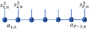
Figure 1: Matrix product state representation of the density matrix of the system as specified in Eq. (10).

In principle, this MPS factorization is exact; however, for an arbitrary density matrix, the maximum spatial bond dimension is $\mathcal{O}\left(d^{P}\right)$. In practice, these bond dimensions are truncated, with the maximum retained dimensionality of each being treated as a convergence parameter. In many cases, it is possible to accurately represent the density matrix with spatial bond dimensions significantly smaller than the theoretical maximum. In fact, if both the initial density matrix and system are separable (i.e., not entangled), the density matrix at all times is exactly represented with a maximum spatial bond dimension of one. In this case, the tensor, $A^{s_{i,n}^{\pm}}_{\alpha_{(i-1,n)},\alpha_{(i,n)}}$, is equivalent to the one-body reduced density matrix of the $i$^th particle after the $n$^th timestep. For cases where the Hamiltonian couples various system sites, the spatial bond dimensions are seen to grow with time, indicating an increase in the entanglement between the sites.

Next, we represent the forward-backward propagator, $K$, in the form of an MPO,

$$K\left(S_{n}^{\pm},S_{n+1}^{\pm},\Delta t\right)= \sum_{\left\{\alpha_{(i,n)}\right\}}W^{s_{1,n}^{\pm},s_{1,n+1}^{\pm}}_{\alpha_{(1,n)}}W^{s_{2,n}^{\pm},s_{2,n+1}^{\pm}}_{\alpha_{(1,n)},\alpha_{(2,n)}}$$

$$\cdots W^{s_{P-1,n}^{\pm},s_{P-1,n+1}^{\pm}}_{\alpha_{(P-2,n)},\alpha_{(P-1,n)}}W^{s_{P,n}^{\pm},s_{P,n+1}^{\pm}}_{\alpha_{(P-1,n)}}.$$ ((11))

As before, the superscripts correspond to the site indices and the subscripts correspond to the spatial bond indices. Unlike the reduced density MPS, which has a single site index ($s_{i,n}^{\pm}$) associated with each tensor, the forward-backward propagator MPO has two ($s_{i,n}^{\pm}$ and $s_{i,n+1}^{\pm}$). The two indices represent the same particle at different time points. Loosely speaking, the tensor, $W^{s_{i,n}^{\pm},s_{i,n+1}^{\pm}}_{\alpha_{(i-1,n)},\alpha_{(i,n)}}$, can be thought of as an effective forward-backward propagator acting on the $i$^th particle.

Generally, any forward-backward propagator can be represented as an MPO, but doing so may be as costly as directly solving the Schrödinger equation. Fortunately, using matrix product representations for studying dynamics of the bare system has been a topic of intense research over the years. Various methods like time-evolving block decimation (TEBD) [47, 48, 5] and time-dependent DMRG (tDMRG) [5, 7] have been developed to directly simulate the time evolution of wave functions of extended systems with short-ranged interactions. For systems with long-ranged interactions, the recently introduced MPO W^I,II method [49] can generate very efficient representations of the propagator. Additionally, a time-dependent variatonal principle (TDVP) [50, 51, 52] approach has also been developed that allows for the treatment of arbitrary Hamiltonians. While TEBD and MPO W^I,II calculate the propagators, Krylov subspace-based methods and TDVP often approximate the action of the propagator on the wave function. Detailed comparisons of these methods for the purposes of simulating the propagator, especially in the context of the current method, is extremely interesting and beyond the scope of this paper. For the current development, we will simply assume that an MPO representation of the forward-backward propagator is available.

To incorporate the Feynman-Vernon influence functional, in the standard TNPI framework, [33, 30, 29, 32] an SVD factorization is performed on the forward-backward system propagator along the time dimension, enabling us to represent the path amplitude tensor as an MPS:

$$P_{S_{0}^{\pm}\cdots S_{N}^{\pm}} =\sum_{\left\{\beta_{n}\right\}}T^{S_{0}^{\pm}}_{\beta_{0}}\cdots T^{S_{n}^{\pm}}_{\beta_{n-1},\beta_{n}}\cdots T_{\beta_{N-1}}^{S_{N}^{\pm}}$$ ((12))

which can be acted upon by the influence functional MPO. Unlike in the MPS decomposition of the density matrix, Eq. (10), the site indices, here, correspond to the forward-backward state of the entire extended system at different time points. The bond indices, $\left\{\beta_{n}\right\}$, represent the coupling between different time points and will be referred to as the temporal bonds for the remainder of this work. More specifically, the dimensionality of the temporal bond indices is related to the length of the non-Markovian memory. In light of this MP factorization of the system described above, Eq. (12) can be rewritten as

$$P_{S_{0}^{\pm}\cdots S_{N}^{\pm}} =\sum_{\left\{\beta_{n}\right\}}\mathbb{T}^{S_{0}^{\pm}}_{\beta_{0}}\cdots\mathbb{T}^{S_{n}^{\pm}}_{\beta_{n-1},\beta_{n}}\cdots\mathbb{T}_{\beta_{N-1}}^{S_{N}^{\pm}},$$ ((13))

where the symbol $\mathbb{T}$ is an MP representation of the corresponding $T$ tensors decomposed along the system or spatial dimension. Thus, we have a product of tensor products, i.e. a 2D array of tensors.

To facilitate this 2D decomposition of the path integral expression, we proceed by using SVD to factor the forward-backward propagator MPO in Eq. (11):

$$W^{s_{1,n}^{\pm},s_{1,n+1}^{\pm}}_{\alpha_{(1,n)}} =\sum_{\beta_{(1,n)}}U^{s_{1,n}^{\pm}}_{\alpha_{(1,n)},\beta_{(1,n)}}R^{s_{1,n+1}^{\pm}}_{\beta_{(1,n)}}$$ ((14))

$$W^{s_{i,n}^{\pm},s_{i,n+1}^{\pm}}_{\alpha_{(i-1,n)},\alpha_{(i,n)}} =\sum_{\beta_{(i,n)}}U^{s_{i,n}^{\pm}}_{\alpha_{(i-1,n)},\alpha_{(i,n)},\beta_{(i,n)}}R^{s_{i,n+1}^{\pm}}_{\beta_{(i,n)}},\medspace 1<i<P$$ ((15))

$$W^{s_{P,n}^{\pm},s_{P,n+1}^{\pm}}_{\alpha_{(P-1,n)}} =\sum_{\beta_{(P,n)}}U^{s_{P,n}^{\pm}}_{\alpha_{(P-1,n)},\beta_{(P,n)}}R^{s_{P,n+1}^{\pm}}_{\beta_{(P,n)}}.$$ ((16))

where $U$ and $R$ are the factors obtained through the SVD procedure. The square-root of diagonal matrix of singular values has been absorbed into the $U$ and $R$ tensors. As per our convention, the bonds along the spatial and temporal dimensions are denoted by $\alpha$ and $\beta$, respectively. Figure 2 shows this structure in the form of a tensor diagram.

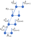
Figure 2: Factorization of the forward-backward MPO following Eqs. (14)–(16)

Now we can put the expressions together to derive the tensors constituting the MPs, $\mathbb{T}$, in Eq. (13). Generally speaking, each of these constituent tensors, represented here by $M$, possesses five indices: one site, $s^{\pm}_{i,n}$, and four bonds ($\alpha_{(i,n)}$, $\beta_{(i,n)}$, $\alpha_{(i-1,n)}$ and $\beta_{(i,n-1)}$), where the values of $i$ and $n$ correspond to the location of the tensor in the 2D grid structure, which is illustrated in Fig. 3. It’s worth noting that the tensors on the edges of the grid have a slightly different structure, as the number of bond indices differ. The tensors corresponding to the initial time point, or equivalently the first column, are given as:

$$M^{s^{\pm}_{1,0}}_{\alpha_{(1,0)},\beta_{(1,0)}} =U^{s^{\pm}_{1,0}}_{\alpha_{(1,0)},\beta_{(1,0)}}$$ ((17))

$$M^{s^{\pm}_{i,0}}_{\alpha_{(i,0)},\beta_{(i,0)},\alpha_{(i-1,0)}} =U^{s^{\pm}_{i,0}}_{\alpha_{(i-1,0)},\alpha_{(i,0)},\beta_{(i,0)}}$$ ((18))

$$M^{s^{\pm}_{P,0}}_{\alpha_{(P-1,0)},\beta_{(P,0)}} =U^{s^{\pm}_{P,0}}_{\alpha_{(P-1,0)},\beta_{(P,0)}}.$$ ((19))

The expressions for the final point, last column:

$$M^{s^{\pm}_{1,N}}_{\beta_{(1,N-1)}} =R^{s^{\pm}_{1,N}}_{\beta_{(1,N-1)}}$$ ((20))

$$M^{s^{\pm}_{i,N}}_{\beta_{(i,N-1)}} =R^{s^{\pm}_{i,N}}_{\beta_{(i,N-1)}}$$ ((21))

$$M^{s^{\pm}_{P,N}}_{\beta_{(P,N-1)}} =R^{s^{\pm}_{P,N}}_{\beta_{(P,N-1)}}.$$ ((22))

Lastly, for an intermediate time point, $n$:

$$M^{s^{\pm}_{1,n}}_{\alpha_{(1,n)},\beta_{(1,n)},\beta_{(1,n-1)}} =R^{s^{\pm}_{1,n}}_{\beta_{(1,n-1)}}U^{s^{\pm}_{1,n}}_{\alpha_{(1,n)},\beta_{(1,n)}}$$ ((23))

$$M^{s^{\pm}_{i,n}}_{\alpha_{(i,n)},\beta_{(i,n)},\alpha_{(i-1,n)},\beta_{(i,n-1)}} =R^{s^{\pm}_{i,n}}_{\beta_{(i,n-1)}}U^{s^{\pm}_{i,n}}_{\alpha_{(i-1,n)},\alpha_{(i,n)},\beta_{(i,n)}}$$ ((24))

$$M^{s^{\pm}_{P,n}}_{\beta_{(P,n)},\alpha_{(P-1,n)},\beta_{(P,n-1)}} =R^{s^{\pm}_{P,n}}_{\beta_{(P,n-1)}}U^{s^{\pm}_{P,n}}_{\alpha_{(P-1,n)},\beta_{(P,n)}}.$$ ((25))

Notice that here, the sites on the final time point are not connected together, Eqs. (20) – (22), inheriting the fundamental asymmetry between the initial and final time points in the structure in Fig. 2.

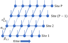
Figure 3: Factorization of the forward-backward MPO.

The flexibility of this factorization becomes apparent when the bath interactions, in form of an IF, are incorporated. The 2D structure discussed till now can be thought of as a series of generalized tensor products along the “columns” that represent the state of the full system at a given time point, or along the “rows” that represent the state of one site at all times (i.e. the path amplitude tensor of that particular site). While thinking of it as a collection of columns manifestly connects the method to its tDMRG heritage, its identification as a collection of “row” tensors serve to illustrate how this multisite method is related to AP-TNPI. [33] (On a different note, in this picture, MPI would be similar to a method that iterates over the rows of this 2D structure.) If there was no interaction between the sites, the rows would separate out and every site would behave like the standard TNPI method. This makes it quite simple to account for the influence functional.

Because we are considering site-local baths, the total IF is just a product of the IFs on each of the sites. The structure of the IF is the same irrespective of the site. Hence, if we consider the path of the $i$^th site as being given by $\left\{s^{\pm}_{i,n}\right\}$, then the IF [8] is:

$$F\left[\left\{s^{\pm}_{i,n}\right\}\right] =\exp\left(-\frac{1}{\hbar}\sum_{0\leq k\leq N}\Delta s_{i,k}\sum_{0\leq k^{\prime}\leq k}(\real(\eta_{kk^{\prime}})\Delta s_{i,k^{\prime}}\right.$$

$$\left.\vphantom{\sum_{0\leq k\leq N}}+2i\imaginary(\eta_{kk^{\prime}})\bar{s}_{i,k^{\prime}})\right)$$ ((26))

where $\Delta s_{i,k}=s^{+}_{i,k}-s^{-}_{i,k}$ and $\bar{s}_{i,k}=\tfrac{s^{+}_{i,k}+s^{-}_{i,k}}{2}$ and $\eta_{kk^{\prime}}$ are the coefficients obtained by discretising the bath response function along the quasi-adiabatic path. [24, 25] It is possible to have different baths associated with different sites leading to a site-dependent $\eta$-coefficient and site-dependent influence functional, however for notational convenience, we describe the method assuming the baths on different sites are characterized by the same spectral density.

We have already discussed the analytical form for the matrix product operator for the IF. [33] Following that procedure, Eq. (26) is factorized based on the $k$ time point:

$$F_{k}\left[\left\{s^{\pm}_{i,n}\right\}\right] =\exp\left(-\frac{1}{\hbar}\Delta s_{i,k}\sum_{0\leq k^{\prime}\leq k}(\real(\eta_{kk^{\prime}})\Delta s_{i,k^{\prime}}\right.$$

$$\left.\vphantom{\sum_{0\leq k\leq N}}+2i\imaginary(\eta_{kk^{\prime}})\bar{s}_{i,k^{\prime}})\right)$$ ((27))

and each $F_{k}$ is given an MPO-representation, $\mathbb{F}_{k}$. The MPOs are applied to each row of the 2D multisite TNPI structure for each system site in order of increasing $k$ as detailed in Ref. [33]. The operations on the first and the last rows (sites) are schematically indicated in Fig. 4.

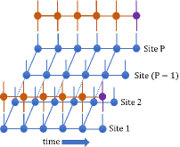
Figure 4: Schematic showing the application of the influence functional MPO to the 2D MS-TNPI structure. Only the influence functionals for the first and the last sites are shown here. Purple vertices correspond to the “projection” operator on the last time point (cf. Ref [33]).

The resulting the tensor network corresponds to the path amplitude tensor. By tracing over the internal system indices as well as contracting all the temporal bonds, we can obtain the AP expressed as an MPO. This is achieved most easily by considering the network as a sequence of columns, each representing the state of the system at a given time point. Tracing over the internal system indices turns these columns into MPOs. From here, the AP MPO is obtained by multiplying all the column MPOs together in a sequential manner, thereby contracting the temporal bonds. By applying this AP MPO to an MPS representing the initial state of the system, we can obtain the corresponding time-evolved final state. This AP-formulation is particularly helpful if we are interested in studying the behaviors of a variety of different initial states. However, usually only the dynamics arising from a specific initial system state is desired. In such cases, we can obtain the resulting final state in a more efficient manner by reducing the problem to one of a sequential application of the column MPOs to the initial state MPS. As MPS-MPO operations are much cheaper than MPO-MPO operations, the AP MPO should not be computed unless it is required. For the examples given here, we will restrict our attention to the MPS-MPO contraction scheme.

It is well-known that for simulations in the condensed phase, the non-Markovian memory does not extend for all of history. This means that the paths can be truncated after $L$ time steps, to simulate a non-Markovian memory of time-span $L\Delta t$. To develop such an iteration procedure, one needs to know the full state of the system at any time point. We have access to that information for the extended system in the form of the column corresponding to the relevant time-point in the 2D lattice structure, Fig. 3. Iteration can also be done in two ways — for the AP as done in Ref. [33], or as typically done, for a particular initial state. [25, 24] Once again in the interest of simplicity of discussion and computational efficiency, we describe the iteration scheme for a particular initial reduced density tensor, $C_{0}=\tilde{\rho}(0)$. For a simulation with memory length $L$, in the iterative regime, there would always be $L+1$ columns, $C_{n}$ for $1\leq n\leq L+1$. The iterative procedure is outlined below. In the following steps for iterative propagation, a tensor contraction is represented by $\otimes$.

1. Update $C_{0}$ by applying the MPO, $C_{1}$ to it. $C_{0}\leftarrow C_{1}\otimes C_{0}$.

2. Copy the other columns in by “sliding them” back by one. $C_{n}\leftarrow C_{n+1}$ for $n<L$.
   Notice at this stage that the new first column is no longer an MPO.

3. Update the second last column, $C_{L}$ by multiplying by the corresponding $U$ tensors obtained from the SVD decomposition of the forward-backward MPO in Eqs. (14)–(16).

4. Insert the last column according to Eqs. (20)–(22).

5. Apply the IF MPO in a row-wise fashion.

6. Trace over the site indices of $C_{1}$ to obtain an MPO in the first column.

The steps 1 through 6 are repeated as many times as required. The salient ideas of the iterative procedure are schematically outlined in Fig. 5.

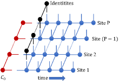
Figure 5: Iteration of the MS-TNPI network. At step (5), notice that the first column is not an MPO. After contraction with identity MPS, it becomes a MPO.

Finally, given the immense difficulty of the problem at hand, it is of interest to estimate the complexity of the algorithm outlined. The two most computationally demanding operations that occur during each time step are the application of the IF MPO and the contraction of the resulting tensor network. Roughly speaking, the cost of applying the IF MPO is $\mathcal{O}\left(m_{t}^{3}w_{p}^{2}w_{I}^{2}d^{2}\right)$ and cost of the contraction is $\mathcal{O}\left(m^{3}w_{p}^{2}m_{t}\right)$. Here, $m_{t}$ is the maximum temporal bond dimension, $m$ is the maximum bond dimension of the contracting MPS, $w_{I}$ is the maximum bond dimension of the IF MPO. The typical bond dimension of the forward-backward propagator of the bare system is denoted by $w_{p}$ and $d$ is the dimensionality of a typical system site. Though the magnitude of $m_{t}$ might be dependent on the memory length, $L$, the exponential growth of complexity within memory is effectively curtailed. [33] Since the local vibrational baths would typically consist of high frequency modes (implying that the non-Markovian memory length, $L$, is not very large), and the site-site couplings would be quite high, the cost would probably be dominated by the contraction process. However, if the local baths are very strongly coupled, the temporal bond dimension would grow much faster than the bond dimension along the system axis, and the pattern would be reversed.

III Results

For the purposes of illustrating the multisite TNPI method, we consider spin chains with nearest-neighbor intersite coupling. The Hamiltonian is given as

$$\hat{H}_{0} =\sum_{i=1}^{P}\hat{h}^{(1)}_{i}+\sum_{i=1}^{P-1}\hat{h}^{(2)}_{i,i+1}$$ ((28))

where

$$\hat{h}^{(1)}_{i} =\epsilon\hat{\sigma}_{z}^{(i)}-\hbar\Omega\hat{\sigma}_{x}^{(i)}$$ ((29))

is the one-body term. The strength of the transverse field is $\hbar\Omega$, and $\epsilon$ represents any asymmetry present in the system due to a longitudinal field. The two-body interaction term is given by a general nearest-neighbor Hamiltonian:

$$\hat{h}^{(2)}_{i,j} =\delta_{j,i+1}\left(J_{x}\hat{\sigma}_{x}^{(i)}\hat{\sigma}_{x}^{(j)}+J_{y}\hat{\sigma}_{y}^{(i)}\hat{\sigma}_{y}^{(j)}+J_{z}\hat{\sigma}_{z}^{(i)}\hat{\sigma}_{z}^{(j)}\right).$$ ((30))

Here, $\hat{\sigma}^{(i)}_{x}$, $\hat{\sigma}^{(i)}_{y}$, $\hat{\sigma}^{(i)}_{z}$ are the Pauli spin matrices on the $i$^th site. Each of the sites is also coupled with its vibrational degrees of freedom described by the harmonic bath given in Eq. (2) with the system-bath coupling operator $\hat{s}_{i}=\hat{\sigma}_{z}^{(i)}$. For the examples shown here, the harmonic bath is characterized by an Ohmic spectral density with an exponential decay:

$$J(\omega) =\frac{\pi}{2}\hbar\xi\omega\exp\left(-\frac{\omega}{\omega_{c}}\right)$$ ((31))

where $\xi$ is the dimensionless Kondo parameter, and $\omega_{c}$ is the characteristic cutoff frequency. In Appendix A, we outline the second-order Suzuki-Trotter splitting TEBD scheme used here to construct the forward-backward propagator MPO.

Depending on the nature of the intersite coupling, there are many models for interacting spin chains. Here, we consider the dynamics of the Ising model, the XXZ model and the Heisenberg model with $P=31$ sites, coupled to site-local harmonic baths. The states of each system site are labeled $\ket{+1}$ and $\ket{-1}$, which are eigenstates of the $\hat{\sigma}_{z}$ operator with eigenvalue of $+1$ and $-1$ respectively. Though the initial condition for MS-TNPI can be any arbitrary reduced density MPS (for example, a DMRG ground state), here for simplicity, it is defined as the direct product state of all spins being in $\ket{+1}$. An SVD compression scheme with a truncation threshold of $\chi$, which is treated as a convergence parameter, is applied to the propagator MPO as well as the results of any MPS-MPO multiplications. Under this scheme, singular values, $\lambda_{n}$, are discarded such that

$$\frac{\sum_{n\in\text{discarded}}\lambda_{n}^{2}}{\sum_{n}\lambda_{n}^{2}}<\chi.$$ ((32))

So, for the following simulations, in addition to the $\Delta t$ and $L$ parameters standard to path integral simulations, $\chi$ is also a convergence parameter. Unlike the single site version, in the most general multisite case, there are two factors that affect the Trotter error, and correspondingly the converged $\Delta t$. First, there is a Trotter error associated with the system-solvent splitting. This is very similar to the single-site case. Additionally, the multisite problem also has a Trotter error associated with the splitting of the bare system propagator under the TEBD scheme.

Transition from an underdamped coherent to a fully incoherent behavior is a hallmark of system-solvent dynamics. Here, we have three different parameters that affect the nature of dynamics — the strength of the intersite coupling (quantifying the ability of the spin chain to act as a self-bath), the strength of the system-solvent coupling, and the temperature.

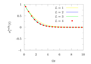
(a) Convergence with respect to $L$ for $\Omega\Delta t=0.25$

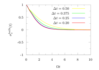
(b) Convergence with respect to $\Delta t$ for $L\Delta t=1$

Figure 6: Covergence of dynamics with respect to various parameters for the Ising model with $J_{z}=1.6$.

III.1 Ising Model

We first consider a transverse-field Ising model ($J_{x}=J_{y}=0$ and $J_{z}\neq 0$) coupled with local vibrations. The longitudinal field is absent, $\epsilon=0$, and a unit transverse field $\Omega=1$ is applied. The dynamics is simulated for different values of the intersite coupling, $J_{z}=\pm 0.2,\pm 0.4,\pm 0.8$ and $\pm 1.6$. Here the bath is characterized by $\xi=0.25$, $\omega_{c}=5\Omega$, and it is held at an inverse temperature of $\hbar\beta\Omega=1$. The convergence of $J_{z}=1.6$ is the most difficult. Therefore, in Fig. 6, we demonstrate the convergence patterns for this parameter.

Figure 7 shows $\expectationvalue{\hat{\sigma}_{z}(t)}$ for the 16^th spin in the chain. We observed that the finite size effects of the chain were limited only to a few edge sites and the dynamics of this middle monomer remained unaffected within the time-span of simulation, implying that this is the bulk dynamics. A timestep of $\Omega\Delta t=0.25$ was found to be converged for Fig. 7 (a)–(c). When the bath was present, a memory length of $L=4$ was used, though acceptable convergence was already achieved at $L=3$. According to Fig. 6, for $|J_{z}|=1.6\hbar\Omega$ (Fig. 7 (d)), $\Omega\Delta t$ was converged at 0.20 and $L$ at 5. A converged compression was done at a cutoff of $\chi=10^{-11}$. The dynamics of the bare system is shown for the various cases in dashed lines. It, unlike the dynamics in presence of the dissipative bath, remains the same irrespective of the sign of $J_{z}$. For the bare dynamics, we could use the MS-TNPI method and it would reduce to a density matrix version of TEBD. However, for efficiency, we propagated the wave function using TEBD with the same cutoff of $\chi=10^{-11}$. In Fig. 7, we see that increasing the intersite couplings leads to a more incoherent dynamics. For the high intersite coupling case, the excess dissipation happens primarily due to the extended Ising chain.

The case of $J_{z}=-0.2\hbar\Omega$ (Fig. 7 (a) red line) was discussed by Makri [40] for a system with 10 sites. We recover identical edge spin dynamics with our method. We observe that the finite size of the chain affects more sites when $J_{z}$ is larger (not shown in figure). This is because, for larger values of $J_{z}$, the sites “know” more about their neighbors, making the difference between an edge site with only one neighbor and a middle site with two neighbors more obvious. It is interesting that, though the difference of sign in the values of $J_{z}$ does not impact the dynamics of the bare system, it leads to profound differences once the bath is coupled. Positive values of $J_{z}$ appear to make the population dissipation faster.

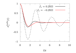
(a) $|J_{z}|=0.2\hbar\Omega$.

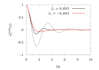
(b) $|J_{z}|=0.4\hbar\Omega$.

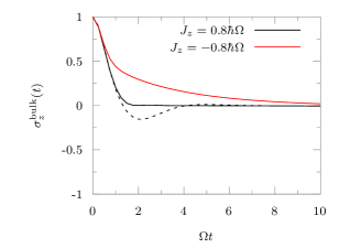
(c) $|J_{z}|=0.8\hbar\Omega$.

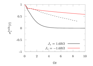
(d) $|J_{z}|=1.6\hbar\Omega$.

Figure 7: Dynamics of a spin in the bulk as represented by $\expectationvalue{\hat{\sigma}_{z}(t)}$ for the 16^th site of the Ising model coupled to an Ohmic bath. Dashed line: without bath.

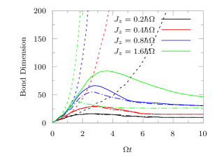
Figure 8: Average bond dimensions of the reduced density MPS for the bare (dashed line) and the full system for various intersite couplings. Positive $J_{z}$ is represented by the full solid line and negative $J_{z}$ by the dot-dashed line.

There are two competing factors that contribute to the computational complexity — the non-Markovian memory caused by the presence of the bath, and the entanglement that develops between the sites as time evolves causing the bond dimension of the MPS to grow. The average bond dimension of the time evolved density matrix can be used as a metric for the entanglement between the sites. In Fig. 8, we show its evolution as a function of time for the parameters shown here. Though for the bare system case shown in Fig. 7, we propagated the wave function, here, for consistency, the density matrix is propagated. We notice that the average bond dimension grows faster for the bare system in comparison to all the cases with the bath, demonstrating the decohering effect brought in by the dissipative medium. Though the bath introduces a memory, it severely restricts the growth of the bond dimension, and equivalently, the entaglement. It is interesting to note that for higher values of interspin couplings, $J_{z}$, the difference in bond dimension between the positive and the negative values increases. This is also reflected in the fact that the dynamics becomes drastically different (cf. Fig. 7(c) and (d)). The eventual decrease in the bond dimension in the presence of a bath reflects its ability to disentangle the system states.

III.2 XXZ Model

Another common model is the so-called XXZ-model, where the two-body interaction term is defined by $J_{x}=J_{y}=J\neq 0$. In absence of any external field, the ratio between $J_{z}$ and $J$ is an order parameter for quantum phase transitions at zero temperature. [53] When $J_{z}<-J$, the ground state is ferromagnetic. There is a disordered spin-liquid phase when $-1<\tfrac{J_{z}}{J}<1$, and finally for $J_{z}>J$, there is an antiferromagnetic state.

Here, we consider an XXZ system in an external transverse field of strength $\Omega=1$ and with a longitudinal field of $\epsilon=0$. The harmonic bath is once again held at an inverse temperature of $\hbar\Omega\beta=1$. However, in these examples, it is characterized by $\xi=0.2$, $\omega_{c}=2$. We consider cases where $J_{z}=\pm 5J$ and $J_{z}=0$. The time-step used for the convergence is $\Omega\Delta t=0.25$. The compression was done at a cutoff of $\chi=10^{-11}$. The dynamics of $\expectationvalue{\hat{\sigma}_{z}(t)}$ for a bulk spin is demonstrated for $J=0.1$ and $J_{x}=0,\pm 0.5$ in Fig. 9.

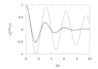
(a) $J=0.1$, $J_{z}=0$.

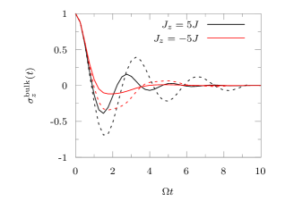
(b) $J=0.1$, $|J_{z}|=0.5$.

Figure 9: Dynamics of a spin in the bulk as represented by $\expectationvalue{\hat{\sigma}_{z}(t)}$ for the 16^th site of the XXZ-model coupled to a harmonic bath. Dashed line: without bath.

We note that the dynamics corresponding to the different values of $J_{z}$ are totally different, even in the absence of the bath. It seems that the dissipation effects increase as the absolute value of $J_{z}$ increases. However, this increase in dissipation does not happen symmetrically. The effects coming from a negative $J_{z}$ are much more pronounced than those caused by a positive value. This difference may owe its origin to the fact that a negative $J_{z}$ stabilizes the initial state of all up spins, whereas positive values of $J_{z}$ destabilizes this state further. Also, the energy spectrum of the bare XXZ system is different in the two cases. These differences and the full effects of vibrational baths are very interesting and deserve a thorough analysis, that will be the subject of future work.

Next, we study the effect of temperature on the dynamics of these XXZ systems. With wave-function methods like DMRG, it becomes especially difficult to do comparatively high temperature simulations because a large number of eigenstates of the bath needs to be accounted for. In Fig. 10, we demonstrate the dynamics of the $J_{z}=0$ system at different temperatures ranging from $\beta=10$ to $\beta=0.1$. Temperature does not affect the converged value of $\Delta t$, but at higher temperatures the memory span needed to fully converge the dynamics increases. As per our intuitive understanding, at higher temperatures, the oscillations get washed away, showing a transition from an underdamped coherent oscillatory dynamics at low temperatures to a fully incoherent dynamics at high temperatures.

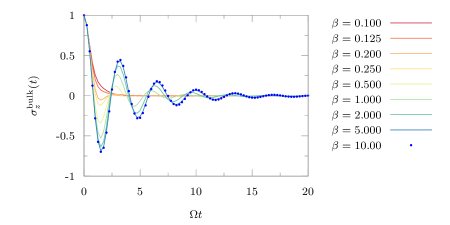
Figure 10: Dynamics of $\expectationvalue{\hat{\sigma}_{z}(t)}$ for the XXZ bulk spin (with $J_{z}=0$) at different temperatures.

III.3 Heisenberg Model

The most general model for interacting spin chains is the so-called “Heisenberg” model. The Hamiltonian is characterized by a two-body spin-spin interaction term that involves independent couplings along $X$, $Y$ and $Z$. The bath used for this example is the same as the one used for the XXZ-model examples.

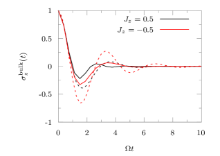
Figure 11: Dynamics of a spin in the bulk represented by $\expectationvalue{\hat{\sigma}_{z}(t)}$ for the 16^th site of the Heisenberg model coupled to a harmonic bath. Dashed line: without bath.

The dynamics of $\expectationvalue{\hat{\sigma}_{z}(t)}$ for a state in the bulk is shown in Fig. 11 for the case of $J_{x}=0,J_{y}=0.1,J_{z}=\pm 0.5$. The simulation was converged at a time-step of $\Omega\Delta t=0.375$, a memory length of $L=3$ and a cutoff of $\chi=10^{-10}$. While we report the dynamics of only the bulk spin here, for the case of $J_{z}=0.5$, our simulations reproduce the previously obtained results [39] for the terminal edge spin.

Next, we explore the dissipation effects of the bath. In Fig. 12, we demonstrate the dynamics of the bulk spin for the case of $J_{z}=0.5$ where the bath is characterized by different Kondo parameters. The dynamics was converged at $L=5$ for $\xi=0.6$ and $\xi=0.8$. The converged time-step $\Omega\Delta t$ remained unchanged at 0.375. One can see the oscillatory nature of the coherent dynamics decrease on increasing the coupling between the system and the bath due to the dissipative effects of the environment.

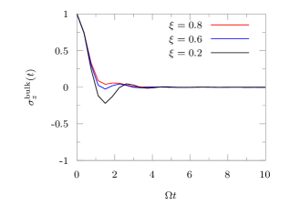
Figure 12: Dynamics of a bulk spin represented by $\expectationvalue{\hat{\sigma}_{z}(t)}$ for the Heisenberg model with $J_{z}=0.5$ and different values of Kondo parameters.

IV Conclusion

System-solvent decomposition is used in various fields of study and is simulated using the Feynman-Vernon influence functional. In such applications there is a necessity to have a low-dimensional quantum system for computational feasibility. However, many interesting problems involve extended systems that can be modeled as collection of many low-dimensional units. Typical examples involve spin-chains to model magnetism and charge or exciton transfers. Such systems have historically been studied without any dissipative environment. Early attempts at applying the same DMRG-based ideas led to interesting applications that resorted to truncating a wave-function description of the environment modes as well. [35] MPI can simulate such extended systems with an associated harmonic bath using Feynman-Vernon influence functionals by iteratively incorporating the various sites to side-step the exponential growth of storage and computational requirements for extended quantum systems. However, it is often useful to simulate the full density matrix, especially for many-body observables. In this paper, we have developed a different approach to simulating these systems by marrying tensor network structures with influence functionals.

Recently, various methods based on tensor networks have been proposed to compress the path integrals, thereby reducing the storage requirements for the simulation. Such compressions, if possible, for multisite systems would especially be especially lucrative because the storage requirements generally grow exponentially with the number of sites. Tensor network path integral methods naturally suggest a further decomposition along the system dimension leading to a multisite method. In this paper, we have introduced a multisite tensor network framework called MS-TNPI, which solves the problem of an extended quantum system coupled with dissipative environments extremely effectively. It is a 2D extension of the 1D MPS structure used in the AP-TNPI [33] or the time-evolving matrix product operators method (TEMPO). [29]

The most essential part of MS-TNPI starts with the definition of a forward-backward propagator for the extended system. This is a common problem that is extensively dealt with in the literature. [6, 35, 5, 47] We show how we can essentially use these propagators and refactorize them to obtain the current 2D structure. We also discuss how by viewing the aforementioned tensor network as a collection of rows containing the path amplitude tensors corresponding to every site, it is now possible to apply the influence functional MPO for the local bath in a systematic manner. Exploration of other existing methods for MPO-MPS style wave function propagation in the current context would be an interesting avenue of research. Especially methods like W^I,II and TDVP, if adapted to the current framework, would enable the simulation of significantly long-ranged interacting systems in presence of local phononic modes. The decoupling of the structure of the system Hamiltonian from the algorithm is an advantage of the current framework.

In general, the MS-TNPI structure can be used to calculate the AP for the extended quantum system. In this paper, however, we have outlined efficient algorithms that focus on using it to generate the full reduced density tensor corresponding to the entire extended system at any point of time in the form of an MPS. MS-TNPI, by its formulation, is also capable of handling arbitrarily complex system initial states represented in the MPS form. While having this global knowledge means that the storage requirements increase with the number of sites, we show that the presence of the local vibrational bath helps decrease the growth of the bond dimension of the reduced density MPS. This feature enables trivial memory iterations corresponding to the finiteness of the non-Markovian memory and efficient evaluation of many-body observables. While the current development uses the analytical form for the influence functionals derived for harmonic baths, it would be interesting to explore the prospects of using the present structure with the more general numerical algorithm for calculating the influence functionals as MPO derived by Ye and Chan.[32]

MS-TNPI is demonstrated through illustrative examples of various spin-chains coupled to local harmonic baths. We simulate the Ising model, the XXZ-model and the Heisenberg model with various different parameters. We show that the site-local baths severely restrict the growth of the bond dimension in the reduced density MPS. Consequently, in comparison to the bare system, the intersite entanglement grows slower and often even decreases in the presence of dissipative environments. We have explored the three different causes of decohering of the system dynamics. There are interesting features of the dynamics for the various phases of the XXZ-model that require further investigation. This would be the subject of future work.

MS-TNPI promises to be an exciting method for extended systems. It makes it possible to study various energy and charge transfer processes, and loss of coherence in chains of qubits. Such applications shall be the focus of our research in the near future. Additionally, the novelty of the structure opens up possibilities for further improvements and developments of which we have only begun scratching the surface.

Authors’ Contributions

Both authors contributed equally to this work.

Data Availability

The data that support the findings of this study are available from the corresponding author upon reasonable request.

Appendix A System Forward-Backward Propagator in MPO representation

For the simple case of nearest-neighbor interacting Hamiltonian, it is very easy to define an algorithm for calculating the second-order Suzuki-Trotter split forward-backward propagator. This is a “forward-backward” version of the second-order time-evolved block decimation scheme. [6]

Let the Hamiltonian be factorized as:

$$\hat{H}_{0}=\sum_{i=1}^{P-1}\hat{\mathcal{H}}_{i,(i+1)}$$ ((33))

where $\hat{\mathcal{H}}_{i,(i+1)}$ takes the one-body term into account as well. To get the second-order splitting, it is usual to incorporate the terminal single body terms fully into the corresponding terms. Everything else is split in halves:

$$\hat{\mathcal{H}}_{1,2} =\hat{h}^{(1)}_{1}+\hat{h}^{(2)}_{1,2}+\frac{1}{2}\hat{h}^{(1)}_{2}$$ ((34))

$$\hat{\mathcal{H}}_{i,(i+1)} =\frac{1}{2}\hat{h}^{(1)}_{i}+\hat{h}^{(2)}_{i,(i+1)}+\frac{1}{2}\hat{h}^{(1)}_{(i+1)},\quad 2\leq i<P-1$$ ((35))

$$\hat{\mathcal{H}}_{(P-1),P} =\frac{1}{2}\hat{h}^{(1)}_{(P-1)}+\hat{h}^{(2)}_{(P-1),P}+\hat{h}^{(1)}_{P}.$$ ((36))

Traditionally, these terms are grouped as “even” and “odd” as follows:

$$\hat{\mathcal{H}}_{\text{odd}} =\sum_{1\leq i<P}^{i\text{ odd}}\hat{\mathcal{H}}_{i,(i+1)}$$ ((37))

$$\hat{\mathcal{H}}_{\text{even}} =\sum_{1\leq i<P}^{i\text{ even}}\hat{\mathcal{H}}_{i,(i+1)},$$ ((38))

where $\hat{\mathcal{H}}_{\text{odd}}$ and $\hat{\mathcal{H}}_{\text{even}}$ do not commute. Under the second order Suzuki-Trotter factorization the forward-backward propagator,

$$K\left(S^{\pm}_{n},S^{\pm}_{n+1},\Delta t\right) \approx\sum_{S^{\pm}_{n^{\prime}},S^{\pm}_{n^{\prime\prime}}}K_{\text{odd}}(S^{\pm}_{n},S^{\pm}_{n^{\prime}},\tfrac{1}{2}\Delta t)$$

$$\times K_{\text{even}}(S^{\pm}_{n^{\prime}},S^{\pm}_{n^{\prime\prime}},\Delta t)$$

$$\times K_{\text{odd}}(S^{\pm}_{n^{\prime\prime}},S^{\pm}_{n+1},\tfrac{1}{2}\Delta t),$$ ((39))

where $S^{\pm}_{n^{\prime}},$ and $S^{\pm}_{n^{\prime\prime}}$ are dummy variables that represent the forward-backward state of the system at the two intermediate time points. In the notation used here, $K_{\text{odd}}(S^{\pm}_{n},S^{\pm}_{n+1},\Delta t)$ and $K_{\text{even}}(S^{\pm}_{n},S^{\pm}_{n+1},\Delta t)$ are the forward-backward propagators associated with $\hat{\mathcal{H}}_{\text{odd}}$ and $\hat{\mathcal{H}}_{\text{even}}$, respectively. The odd and even terms commute with themselves, so the forward-backward propagators can be factorized further:

$$K_{\text{odd}}\left(S^{\pm}_{n},S^{\pm}_{n+1},\Delta t\right)= \prod_{1\leq i<P}^{i\text{ odd}}$$

$$K_{i}(s^{\pm}_{i,n},s^{\pm}_{i+1,n},s^{\pm}_{i,n+1},s^{\pm}_{i+1,n+1},\Delta t)$$ ((40))

$$K_{\text{even}}\left(S^{\pm}_{n},S^{\pm}_{n+1},\Delta t\right)= \prod_{1\leq i<P}^{i\text{ even}}$$

$$K_{i}(s^{\pm}_{i,n},s^{\pm}_{i+1,n},s^{\pm}_{i,n+1},s^{\pm}_{i+1,n+1},\Delta t),$$ ((41))

where the two-body forward-backward propagator,

$$K_{i}(s^{\pm}_{i,n} ,s^{\pm}_{i+1,n},s^{\pm}_{i,n+1},s^{\pm}_{i+1,n+1},\Delta t)=$$

$$\matrixelement{s^{+}_{i,n+1},s^{+}_{i+1,n+1}}{\exp\left(-\frac{i}{\hbar}\hat{\mathcal{H}}_{i,(i+1)}\Delta t\right)}{s^{+}_{i,n},s^{+}_{i+1,n}}$$

$$\times\matrixelement{s^{-}_{i,n},s^{-}_{i+1,n}}{\exp\left(\frac{i}{\hbar}\hat{\mathcal{H}}_{i,(i+1)}\Delta t\right)}{s^{-}_{i,n+1},s^{-}_{i+1,n+1}}.$$ ((42))

Using an SVD, we can factor this two-body (multi-site) operator into a pair of single-body (single-site) operators:

$$K_{i}(s^{\pm}_{i,n}, s^{\pm}_{i+1,n},s^{\pm}_{i,n+1},s^{\pm}_{i+1,n+1},\Delta t)=$$

$$\sum_{\alpha_{(i,n)}}W^{s^{\pm}_{i,n},s^{\pm}_{i,n+1}}_{\alpha_{(i,n)}}W^{s^{\pm}_{i+1,n},s^{\pm}_{i+1,n+1}}_{\alpha_{(i,n)}}.$$ ((43))

Plugging this expression into Eqs. (40) and  (41) gives:

$$K_{\text{odd}}\left(S^{\pm}_{n},S^{\pm}_{n+1},\Delta t\right)= \prod_{1\leq i<P}^{i\text{ odd}}\left(\sum_{\alpha_{(i,n)}}W^{s^{\pm}_{i,n},s^{\pm}_{i,n+1}}_{\alpha_{(i,n)}}W^{s^{\pm}_{i+1,n},s^{\pm}_{i+1,n+1}}_{\alpha_{(i,n)}}\right)$$ ((44))

$$K_{\text{even}}\left(S^{\pm}_{n},S^{\pm}_{n+1},\Delta t\right)= \prod_{1\leq i<P}^{i\text{ even}}\left(\sum_{\alpha_{(i,n)}}W^{s^{\pm}_{i,n},s^{\pm}_{i,n+1}}_{\alpha_{(i,n)}}W^{s^{\pm}_{i+1,n},s^{\pm}_{i+1,n+1}}_{\alpha_{(i,n)}}\right).$$ ((45))

Notice that by introducing unit-dimensional bond indices between the products, they can be reduced to proper MPOs. Thus, the resulting MPOs would have alternating bonds of unit dimension. Finally, the full second order Suzuki-Trotter split forward-backward propagator can be obtained through sequential MPO-MPO multiplications involving Eqs. (44) and (45) as per Eq. (39).

References

- White [1992] S. R. White, “Density matrix formulation for quantum renormalization groups,” Phys. Rev. Lett. 69, 2863–2866 (1992).
- Schollwöck [2005] U. Schollwöck, “The density-matrix renormalization group,” Rev. Mod. Phys. 77, 259–315 (2005).
- Schollwöck [2011a] U. Schollwöck, “The density-matrix renormalization group: A short introduction,” Philos. Trans. A Math. Phys. Eng. Sci. 369, 2643–2661 (2011a).
- Schollwöck [2011b] U. Schollwöck, “The density-matrix renormalization group in the age of matrix product states,” Ann. Phys. (N. Y.) 326, 96–192 (2011b).
- White and Feiguin [2004] S. R. White and A. E. Feiguin, “Real-Time Evolution Using the Density Matrix Renormalization Group,” Phys. Rev. Lett. 93 (2004), 10.1103/physrevlett.93.076401.
- Paeckel et al. [2019] S. Paeckel, T. Köhler, A. Swoboda, S. R. Manmana, U. Schollwöck, and C. Hubig, “Time-evolution methods for matrix-product states,” Ann. Phys. (N. Y.) 411, 167998 (2019).
- Xie et al. [2019] X. Xie, Y. Liu, Y. Yao, U. Schollwöck, C. Liu, and H. Ma, “Time-dependent density matrix renormalization group quantum dynamics for realistic chemical systems,” J. Chem. Phys. 151, 224101 (2019).
- Feynman and Vernon [1963] R. P. Feynman and F. L. Vernon, “The theory of a general quantum system interacting with a linear dissipative system,” Ann. Phys. (N. Y.) 24, 118–173 (1963).
- Tanimura and Kubo [1989] Y. Tanimura and R. Kubo, “Time Evolution of a Quantum System in Contact with a Nearly Gaussian-Markoffian Noise Bath,” J. Phys. Soc. Jpn. 58, 101–114 (1989).
- Duan et al. [2017] C. Duan, Q. Wang, Z. Tang, and J. Wu, “The study of an extended hierarchy equation of motion in the spin-boson model: The cutoff function of the sub-Ohmic spectral density,” J. Chem. Phys. 147, 164112 (2017).
- Ikeda and Scholes [2020] T. Ikeda and G. D. Scholes, “Generalization of the hierarchical equations of motion theory for efficient calculations with arbitrary correlation functions,” J. Chem. Phys. 152, 204101 (2020).
- Popescu, Rahman, and Kleinekathöfer [2016] B. Popescu, H. Rahman, and U. Kleinekathöfer, “Chebyshev Expansion Applied to Dissipative Quantum Systems,” J. Phys. Chem. A 120, 3270–3277 (2016).
- Tanimura [2020] Y. Tanimura, “Numerically “exact” approach to open quantum dynamics: The hierarchical equations of motion (HEOM),” J. Chem. Phys. 153, 020901 (2020).
- Shi et al. [2018] Q. Shi, Y. Xu, Y. Yan, and M. Xu, “Efficient propagation of the hierarchical equations of motion using the matrix product state method,” The Journal of Chemical Physics 148, 174102 (2018).
- Yan, Xing, and Shi [2020] Y. Yan, T. Xing, and Q. Shi, “A new method to improve the numerical stability of the hierarchical equations of motion for discrete harmonic oscillator modes,” The Journal of Chemical Physics 153, 204109 (2020).
- Yan et al. [2021] Y. Yan, M. Xu, T. Li, and Q. Shi, “Efficient propagation of the hierarchical equations of motion using the Tucker and hierarchical Tucker tensors,” The Journal of Chemical Physics 154, 194104 (2021).
- Segal, Millis, and Reichman [2010] D. Segal, A. J. Millis, and D. R. Reichman, “Numerically exact path-integral simulation of nonequilibrium quantum transport and dissipation,” Physical Review B 82 (2010), 10.1103/physrevb.82.205323.
- Simine and Segal [2013] L. Simine and D. Segal, “Path-integral simulations with fermionic and bosonic reservoirs: Transport and dissipation in molecular electronic junctions,” The Journal of Chemical Physics 138, 214111 (2013).
- Banerjee and Makri [2013] T. Banerjee and N. Makri, “Quantum-Classical Path Integral with Self-Consistent Solvent-Driven Reference Propagators,” J. Phys. Chem. B 117, 13357–13366 (2013).
- Lambert and Makri [2012a] R. Lambert and N. Makri, “Quantum-classical path integral. I. Classical memory and weak quantum nonlocality,” J. Chem. Phys. 137, 22A552 (2012a).
- Lambert and Makri [2012b] R. Lambert and N. Makri, “Quantum-classical path integral. II. Numerical methodology,” J. Chem. Phys. 137, 22A553 (2012b).
- Walters and Makri [2015] P. L. Walters and N. Makri, “Quantum–Classical Path Integral Simulation of Ferrocene–Ferrocenium Charge Transfer in Liquid Hexane,” J. Phys. Chem. Lett. 6, 4959–4965 (2015).
- Walters and Makri [2016] P. L. Walters and N. Makri, “Iterative quantum-classical path integral with dynamically consistent state hopping,” J. Chem. Phys. 144, 044108 (2016).
- Makri and Makarov [1995a] N. Makri and D. E. Makarov, “Tensor propagator for iterative quantum time evolution of reduced density matrices. I. Theory,” J. Chem. Phys. 102, 4600–4610 (1995a).
- Makri and Makarov [1995b] N. Makri and D. E. Makarov, “Tensor propagator for iterative quantum time evolution of reduced density matrices. II. Numerical methodology,” J. Chem. Phys. 102, 4611–4618 (1995b).
- Makri [2014] N. Makri, “Blip decomposition of the path integral: Exponential acceleration of real-time calculations on quantum dissipative systems,” J. Chem. Phys. 141, 134117 (2014).
- Makri [2016] N. Makri, “Blip-summed quantum–classical path integral with cumulative quantum memory,” Faraday Discuss. 195, 81–92 (2016).
- Makri [2017] N. Makri, “Iterative blip-summed path integral for quantum dynamics in strongly dissipative environments,” J. Chem. Phys. 146, 134101 (2017).
- Strathearn et al. [2018] A. Strathearn, P. Kirton, D. Kilda, J. Keeling, and B. W. Lovett, “Efficient non-Markovian quantum dynamics using time-evolving matrix product operators,” Nat. Commun 9 (2018), 10.1038/s41467-018-05617-3.
- Jørgensen and Pollock [2019] M. R. Jørgensen and F. A. Pollock, “Exploiting the Causal Tensor Network Structure of Quantum Processes to Efficiently Simulate Non-Markovian Path Integrals,” Phys. Rev. Lett. 123 (2019), 10.1103/physrevlett.123.240602.
- Gribben et al. [2020] D. Gribben, A. Strathearn, J. Iles-Smith, D. Kilda, A. Nazir, B. W. Lovett, and P. Kirton, “Exact quantum dynamics in structured environments,” Phys. Rev. Res. 2 (2020), 10.1103/physrevresearch.2.013265.
- Ye and Chan [2021] E. Ye and G. K.-L. Chan, “Constructing tensor network influence functionals for general quantum dynamics,” J. Chem. Phys. 155, 044104 (2021).
- Bose and Walters [2021] A. Bose and P. L. Walters, “A tensor network representation of path integrals: Implementation and analysis,” arXiv pre-print server (2021).
- Bose [2021] A. Bose, “A Pairwise Connected Tensor Network Representation of Path Integrals,” arXiv pre-print server (2021).
- Ren, Shuai, and Kin-Lic Chan [2018] J. Ren, Z. Shuai, and G. Kin-Lic Chan, “Time-Dependent Density Matrix Renormalization Group Algorithms for Nearly Exact Absorption and Fluorescence Spectra of Molecular Aggregates at Both Zero and Finite Temperature,” J. Chem. Theory Comput. 14, 5027–5039 (2018).
- Makri [2018a] N. Makri, “Communication: Modular path integral: Quantum dynamics via sequential necklace linking,” J. Chem. Phys. 148, 101101 (2018a).
- Makri [2018b] N. Makri, “Modular path integral methodology for real-time quantum dynamics,” J. Chem. Phys. 149, 214108 (2018b).
- Kundu and Makri [2019] S. Kundu and N. Makri, “Modular path integral for discrete systems with non-diagonal couplings,” J. Chem. Phys. 151, 074110 (2019).
- Kundu and Makri [2020a] S. Kundu and N. Makri, “Modular path integral for finite-temperature dynamics of extended systems with intramolecular vibrations,” J. Chem. Phys. 153, 044124 (2020a).
- Makri [2021] N. Makri, “Small matrix modular path integral: Iterative quantum dynamics in space and time,” Phys. Chem. Chem. Phys. 23, 12537–12540 (2021).
- Kundu and Makri [2020b] S. Kundu and N. Makri, “Real-Time Path Integral Simulation of Exciton-Vibration Dynamics in Light-Harvesting Bacteriochlorophyll Aggregates,” J. Phys. Chem. Lett. 11, 8783–8789 (2020b).
- Kundu and Makri [2021] S. Kundu and N. Makri, “Exciton–Vibration Dynamics in J-Aggregates of a Perylene Bisimide from Real-Time Path Integral Calculations,” J. Phys. Chem. C 125, 201–210 (2021).
- Lerose, Sonner, and Abanin [2021] A. Lerose, M. Sonner, and D. A. Abanin, “Influence Matrix Approach to Many-Body Floquet Dynamics,” Phys. Rev. X 11 (2021), 10.1103/physrevx.11.021040.
- Fishman, White, and Stoudenmire [2020] M. Fishman, S. R. White, and E. M. Stoudenmire, “The ITensor Software Library for Tensor Network Calculations,” arXiv pre-print server (2020).
- Caldeira and Leggett [1983] A. O. Caldeira and A. J. Leggett, “Path integral approach to quantum Brownian motion,” Physica A: Statistical Mechanics and its Applications 121, 587–616 (1983).
- Makri [1999] N. Makri, “The Linear Response Approximation and Its Lowest Order Corrections: An Influence Functional Approach,” J. Phys. Chem. B 103, 2823–2829 (1999).
- Daley et al. [2004] A. J. Daley, C. Kollath, U. Schollwöck, and G. Vidal, “Time-dependent density-matrix renormalization-group using adaptive effective Hilbert spaces,” J. Stat. Mech. Theory Exp. 2004, P04005 (2004).
- Vidal [7] G. Vidal, “Efficient Simulation of One-Dimensional Quantum Many-Body Systems,” Phys. Rev. Lett. 93, 040502 (7).
- Zaletel et al. [4] M. P. Zaletel, R. S. K. Mong, C. Karrasch, J. E. Moore, and F. Pollmann, “Time-evolving a matrix product state with long-ranged interactions,” Phys. Rev. B 91, 165112 (4).
- Haegeman et al. [2011] J. Haegeman, J. I. Cirac, T. J. Osborne, I. Pižorn, H. Verschelde, and F. Verstraete, “Time-Dependent Variational Principle for Quantum Lattices,” Phys. Rev. Lett. 107, 070601 (2011).
- Orús [2014] R. Orús, “A practical introduction to tensor networks: Matrix product states and projected entangled pair states,” Ann. Phys. (N. Y.) 349, 117–158 (2014).
- Yang and White [2020] M. Yang and S. R. White, “Time-dependent variational principle with ancillary Krylov subspace,” Phys. Rev. B 102, 094315 (2020).
- Rakov and Weyrauch [10] M. V. Rakov and M. Weyrauch, “Spin-½ XXZ Heisenberg chain in a longitudinal magnetic field,” Phys. Rev. B 100, 134434 (10).