Quantifying Grid Resilience Against Extreme Weather Using Large-Scale Customer Power Outage Data

Abstract

In recent decades, the weather around the world has become more irregular and extreme, often causing large-scale extended power outages. Resilience—the capability of withstanding, adapting to, and recovering from a large-scale disruption—has become a top priority for the power sector. However, the understanding of power grid resilience still stays on the conceptual level mostly or focuses on particular components, yielding no actionable results or revealing few insights on the system level. This study provides a quantitatively measurable definition of power grid resilience, using a statistical model inspired by patterns observed from data and domain knowledge. We analyze a large-scale quarter-hourly historical electricity customer outage data and the corresponding weather records, and draw connections between the model and industry resilience practice. We showcase the resilience analysis using three major service territories on the east coast of the United States. Our analysis suggests that cumulative weather effects play a key role in causing immediate, sustained outages, and these outages can propagate and cause secondary outages in neighboring areas. The proposed model also provides some interesting insights into grid resilience enhancement planning. For example, our simulation results indicate that enhancing the power infrastructure in a small number of critical locations can reduce nearly half of the number of customer power outages in Massachusetts. In addition, we have shown that our model achieves promising accuracy in predicting the progress of customer power outages throughout extreme weather events, which can be very valuable for system operators and federal agencies to prepare disaster response.

1 Introduction

Extreme weather events, such as hurricanes, winter storms, and tornadoes, have become a major cause of large-scale electric power outages in recent years [20, 25]. For example, in March 2018, when the northeastern United States was hit by three winter storms in just 14 days, power failures across the New England region affected more than 2,755,000 customers, causing total economic losses of $4 billion, including $2.9 billion in insured losses [12]. Such extreme weather events often left millions of people without electricity for days, caused substantial economical losses [35, 48], and in some cases even cost human lives [46]. In light of the extensive losses from extreme weather since the early 2000s, United States regulatory entities at different levels have requested the industry to investigate power grid resilience and adopt hardening measures [1, 35]. Consequently, an accurate assessment of power grid resilience has great importance for estimating extreme weather damages, carrying out short-term disaster response to reduce losses, planning long-term resilience enhancement, and making energy policy.

However, the study of grid resilience has been plagued by two major challenges [24, 52]. First, there is a profound disconnect between the real-world power failure data that researchers need and what is available to them. On the one hand, utility companies and system operators may collect fine-grained data on failure and recovery, mainly for reporting purposes, but these are generally not shared outside service territories [9]. On the other hand, U.S. federal and state governments require only aggregated information, such as the total duration of customer service interruptions, from investor-owned service regions during major storms [11]. These data are often aggregated into daily statistics over an entire region that are too crude for use in studying the resilience of infrastructure and services [35]. Apart from data scarcity, studies are also hampered by a lack of mathematical models that can capture the intricate dynamics of disruption and restoration processes under the impact of weather. Because the power grid is a complex and chaotic system [18], the comprehensive and continuous influence of extreme weather incidents on one part of the system can accumulate and magnify to cause large effects on the system as a whole. As a result, identifying all the factors that contribute to massive blackouts has long been a very complicated problem.

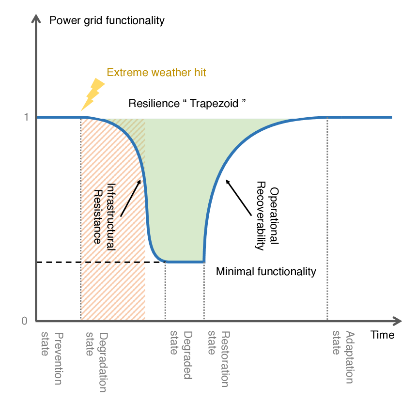
(a)

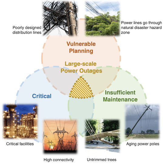
(b)

Figure 1: The resilience conceptual illustration. (a) An illustration of the concept of the resilience curve (green area). The horizontal and vertical coordinates represent time and power grid performance, respectively. The red shaded area represents the time period affected by the extreme weather. The blue line represents power grid performance during an extreme weather incident, where the timeline can be divided into five states based on the status of the power grid: pre-disturbance, performance degradation, degraded state, restoration, and adaptation. Power grid resilience in this study consists of two key characteristics: infrastructure resistance to extreme weather disruptions and operational recoverability from damage. (b) The three key factors, from infrastructure resistance perspective, captured by the proposed model that are closely tied to large-scale power outage: insufficient design margin, insufficient maintenance, and topological criticality in power network.

To circumvent these challenges and bridge this research gap, this paper studies power grid resilience to extreme weather quantitatively by taking advantage of a unique set of fine-grained customer-level power outage records and comprehensive weather data collected from three weather events covering four U.S. states (see Methods). Unlike detailed power grid facility outage records, which are normally inaccessible to the public, customer-level power outage records reported by local utilities [2, 17, 42] are an important data source that are easily accessible but often overlooked. The data record the number of customers without power in each geographical unit (town, county or zip code) every 15 minutes, portraying the entire evolution of several massive blackouts and providing sufficient information to capture the spatio-temporal interactions between disruption and restoration processes. The High-Resolution Rapid Refresh (HRRR) archive [7, 8] is another publicly available data set that provides comprehensive and fine-grained near-real-time weather information estimated by the National Centers for Environmental Prediction’s (NCEP) HRRR data assimilation model. Armed with this data, we developed a statistical model for the progress of customer outages without detailed disruption and restoration records (see Methods). The model aims to capture the intricate spatio-temporal dynamics of customer outages between geographical units and over time based on a multivariate random process. Using the fitted model, we first present a descriptive analysis that demonstrates the existence of grid resilience from real data and shows that the cumulative weather effect plays a pivotal role in creating large-scale power outages. The proposed model also leads to a general definition of power grid resilience, as shown in Figure 1, which can be quantitatively measured by the fitted model’s parameters in four general areas: design margin, maintenance sufficiency, topological criticality, and recoverability. Our model suggests that local power outages directly induced by extreme weather are a non-linear response to cumulative weather effects and cause subsequent large-scale and long-duration blackout by propagating failures through critical nodes in power networks. The model suggests that large-scale power outages can be effectively mitigated by isolating or de-escalating a small set of nodes in the power network.

Related work

The study of grid resilience has become quite popular in recent years [5, 6, 24, 52]. The existing works on resilience evaluation usually fall into two groups: qualitative methods and quantitative methods.

Most studies focus on qualitative resilience evaluation methods. For example, [13, 31, 38] provide frameworks for system- and regional-level resilience overviews using investigation, questionnaires, and individual ratings to address the personal, business, governmental, and infrastructure aspects of resilience. The scoring matrix formulated in [45] evaluates the system function from different perspectives, and analytic methods such as analytic hierarchy process can be conveniently carried out to turn subjective opinions into comparable quantities that are easy to use in decision making [36]. These qualitative frameworks can serve as guidance for long-term energy policy making, as they provide a generally thorough picture of the system. However, there are recent signs that qualitative methods are becoming increasingly expensive and difficult to carry out given the surge in large-scale blackouts over the past decade due to climate change. In addition, these methods are hindered by a lack of scientific evidence to justify the methods adopted in some scenarios.

Quantitative methods, on the other hand, are often based on the quantification of system performance. Due to insufficient access to real-world data [22], quantitative approaches to investigating and modeling the resilience of actual power grids to weather events are still at a nascent stage and not well established. Previous studies, such as [39, 40, 50], attempt to quantify grid resilience by introducing operational and infrastructure resilience metrics based on a variety of indicators, usually requiring detailed disruption and restoration records at each phase. Some other works attempt to tackle this by using a statistical approach without sufficient failure and recovery data. Monte Carlo simulation is used in [4, 39, 51] to assess the capability of the grid and quantify the impact of extreme weather. Recently, a few studies [16, 21, 23] have made significant progress in analyzing specific aspects of power grid resilience or a particular extreme weather event by taking advantage of the limited amount of aggregated power failure data. However, a resilience study that systematically explores customer power outage data, quantitatively analyzes different weather effects on power systems, and evaluates power grid resilience across multiple service territories, does not exist.

Other recent theoretical studies, such as [15], have pointed out that the power grid is vulnerable to massive blackouts, and such vulnerability can be attributed to a very small set of facilities and external factors [53]. Identifying the characteristics of these small sets would be very useful for the analysis and enhancement of resilience to weather events, but related quantitative studies of the real-world power grid are extremely scarce.

2 Real-world example of grid resilience

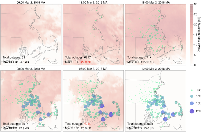
Figure 2: Weather intensity and power outage evolution during the nor’easter March 2-3, 2018, in Massachusetts. These snapshots show outages and weather at six-hour intervals. Each bubble corresponds to a geographical unit. The size and color depth of each bubble represent the number of reported customer power outages per 15-minute interval. The depth of the red cloud over the map represents the level of derived radar reflectivity (REFD) in the corresponding region, which indicates the intensity of the storm. The total number of customer power outages and the maximum REFD in the region of the map for each snapshot are shown in the lower left of the figure. The largest total number of outages and the maximum REFD over this period is highlighted in red.

We will begin by illustrating power grid resilience with a real example, shown in Figure 2. It describes a typical large-scale blackout during a nor’easter (winter storm) that mainly affected eastern Massachusetts in early March 2018. The storm began in the early morning of March 2 and peaked around noon. The peak wind gust reached hurricane level (about 97 miles per hour) and the storm brought strong precipitation (maximum REFD was 27.9 dB). A large-scale power failure appeared in this area almost 18 hours after the storm peak and eventually knocked out power to 4.21 million customers in Massachusetts, with 53 out of 351 cities having more than 50% of their customers without power (Figure 3), according to the outage records. By that time, the storm had greatly weakened and had started moving out of Massachusetts.

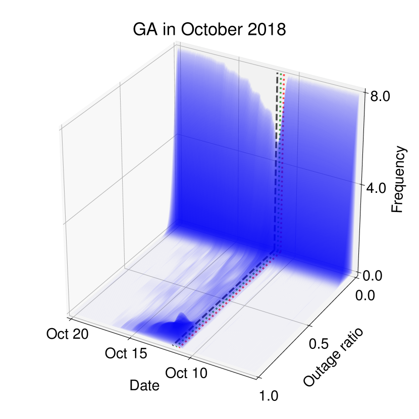
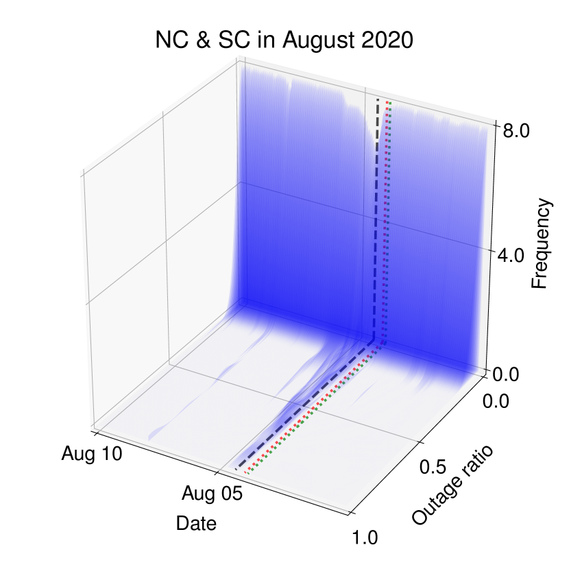
Figure 3: Empirical customer power outage ratio distribution in three major service territories. Black dashed lines indicate the moment when the number of customer power outages in the system reached its peak during the incident. Red and green dotted lines indicate the moment when the weather intensity (REFD and wind, respectively) reached their peak during the extreme weather incident.

We find similar behaviour in other extreme weather events, as illustrated in Figure 3, in which the occurrence of large-scale power outages is normally 12-36 hours behind the peak of the extreme weather. The time lag between extreme weather and large-scale power outages is a result of the existing power grid’s resilience and can be explained by the following four factors:

1. Severe power disruptions are the result of cumulative damage to the power system due to the effects of the extreme weather, which usually builds over time. According to recent outage reports [11, 14, 19, 25], these customer outages are mostly caused by damage to distribution systems. Much of the transmission and distribution network across the United States, particularly in the Midwest and eastern regions, is still above ground, leaving it vulnerable to the effects of extreme weather [25]. Continuous rainfall and constant strong winds exert pressure on trees and utility poles over time, and eventually, utility poles may fall, downed trees could bring down power lines, or continuous precipitation could raise water levels and lead to flooding and damage to transformers.

2. Rather than being immediately affected or damaged by extreme weather, some areas may see outages hours or even days later caused by power failures in other, connected, areas of the system. This outage interdependence or propagation phenomenon can often be observed in the transmission network infrastructure, which typically consists of a meshed transmission network carrying a significant amount of power (typically more than 100 MVA per transmission line). In this case, the loss of one transmission line will congest other adjacent lines, and what’s worse, will cause load shedding in a remote load center due to severe congestion on the remaining lines.

3. Utility companies and system operators are obliged to plan timely restoration for critical power facilities and impose preemptive measures in response to potential damages. These operational restoration activities conducted throughout the electricity service downtime can slow the process of a large-scale power outage.

4. The power grid has a certain disruption tolerance capacity (DTC) within which the power grid can withstand external impacts without power outages. For example, a transmission system operated under N-1 requirements [37] is guaranteed to still be secure after losing any one component. Power grid facilities are also designed with safety margins that enable them to endure external hazards up to a certain point. The accumulation of weather impacts, including rainfall, wind, or snow, normally takes hours or even days to exceed the DTC of a power system, after which large-scale outages begin to occur.

Throughout the electricity service downtime, as we see from the example, power grid resilience plays a crucial role in withstanding impacts from extreme weather, slowing the propagation of blackouts, and bringing blacked out areas back to normal. Based on these observations, we developed a model that aimed to capture the intricate relationship between the number of outages and the extreme weather effect. We will present an analysis based on the fitted model that quantitatively describes the damage caused by extreme weather and intuitively explains how the system reacts to and recovers from these damages.

3 Grid resilience modeling

This section presents a data-driven spatio-temporal model of customer power outages that captures the dynamics of customer power outages across a region. First, we will investigate the impact of extreme weather and define the cumulative weather effect, and then we will propose a spatio-temporal model for the number of customer power outages across the service territory.

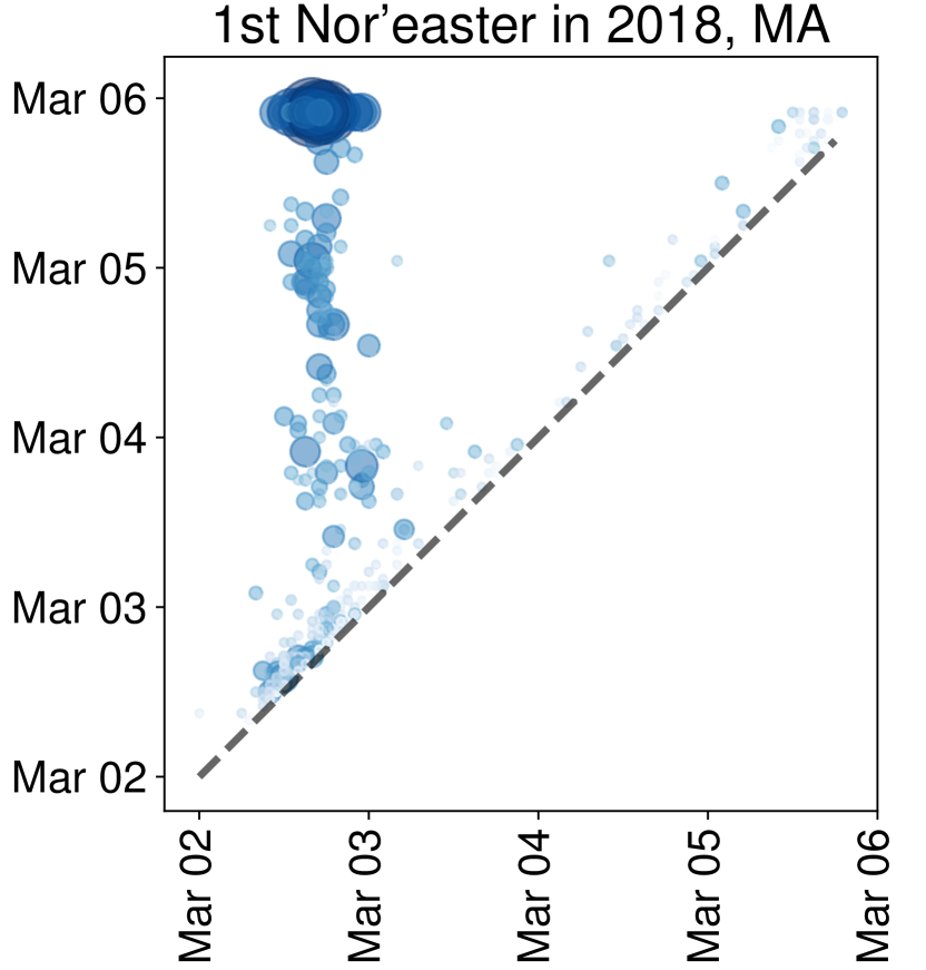
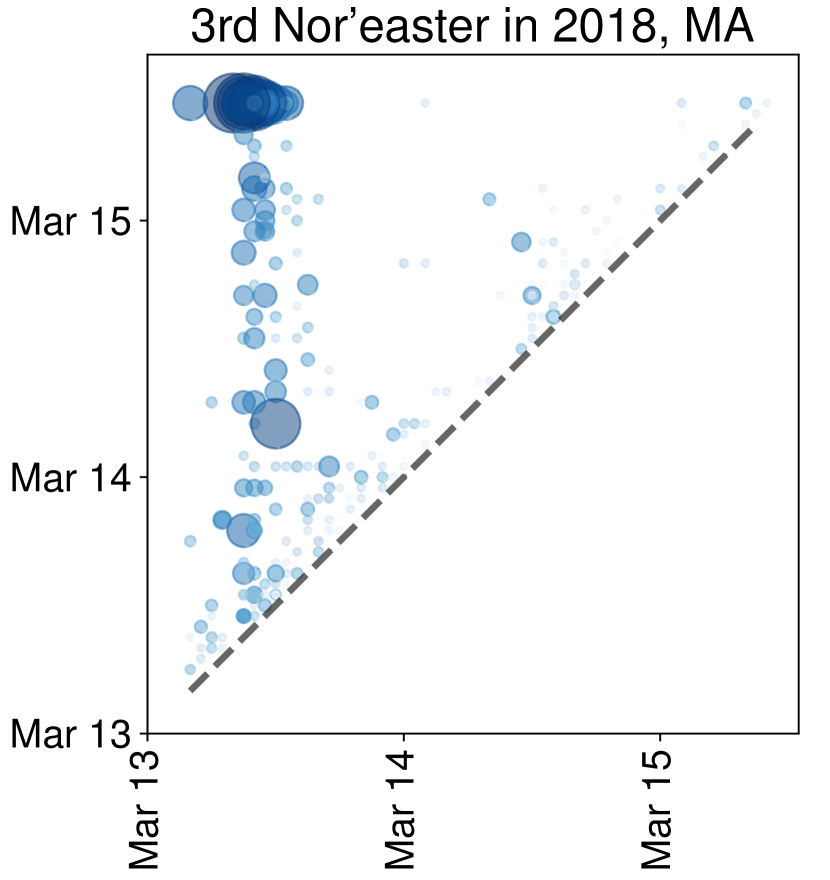
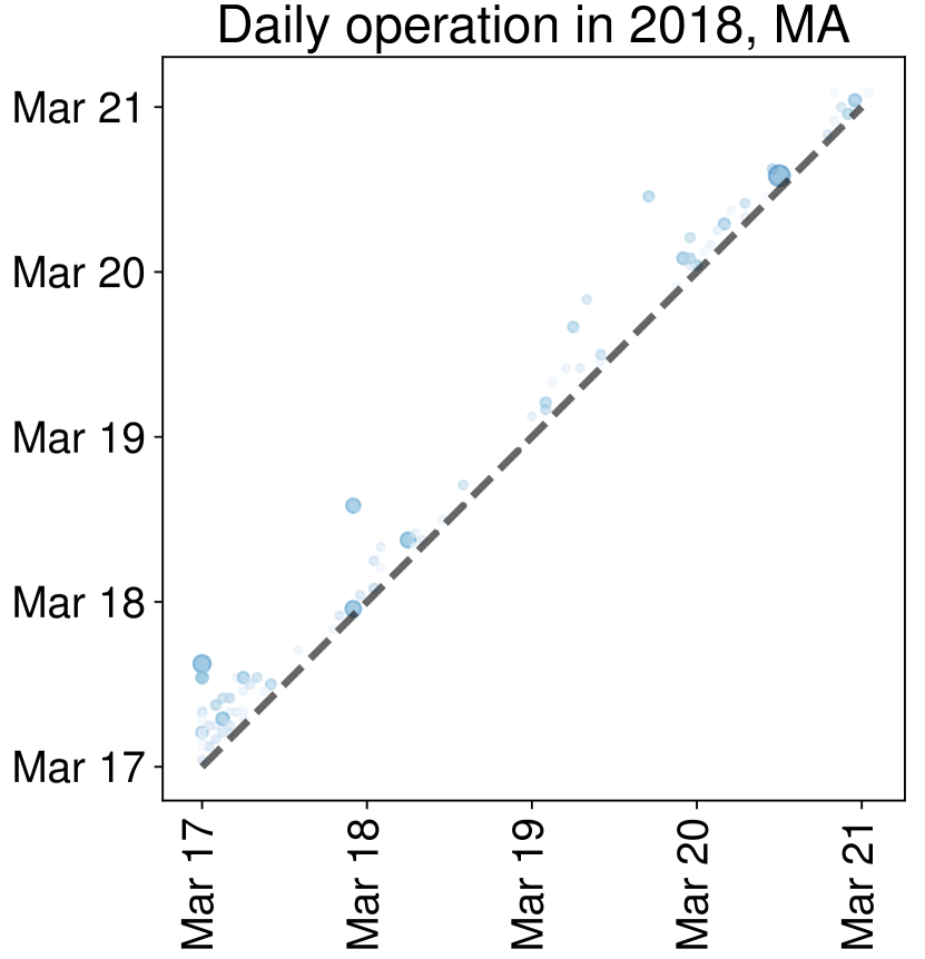
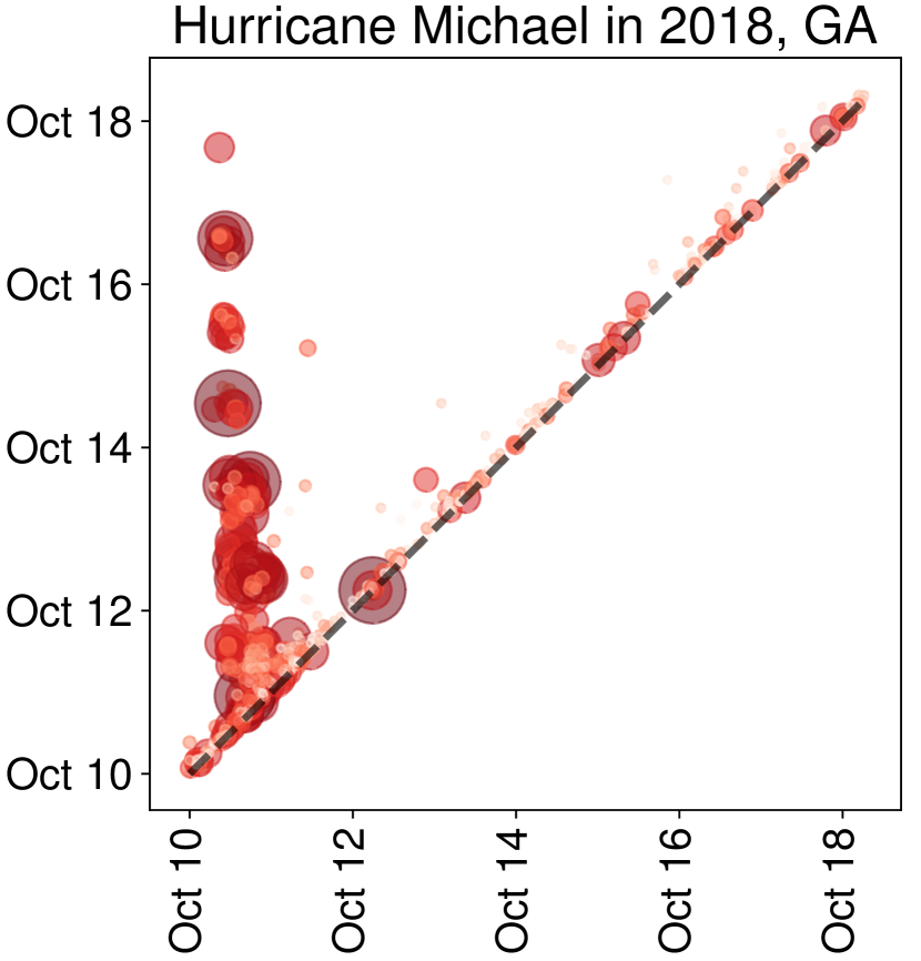
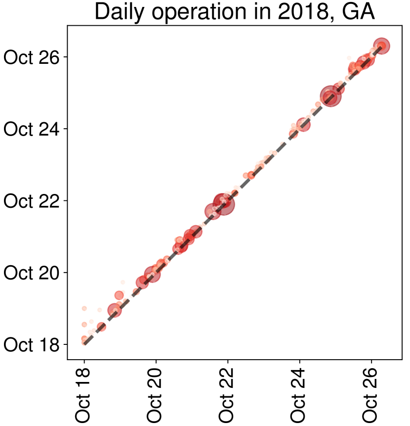
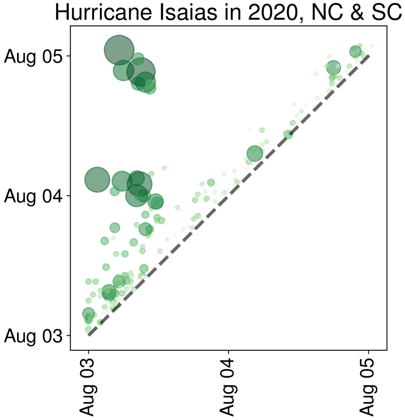
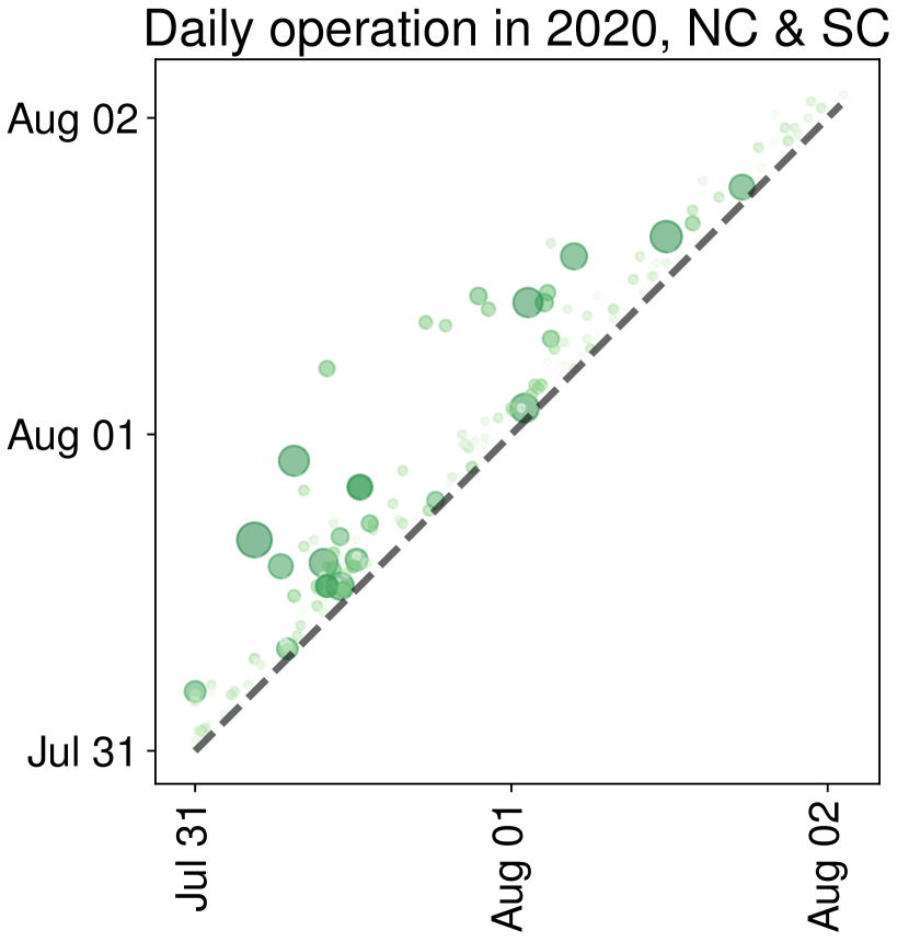
Figure 4: Scatter plots of the duration of the restoration state during five extreme weather events and daily operations. Each bubble corresponds to the duration of the restoration state in a geographical unit. The horizontal and vertical coordinates correspond to the start and end time of the restoration, respectively. The distance of the bubbles from the diagonal line indicates the length of the restoration state. The diagonal dashed line represents the length of the restoration state at zero. Bubble sizes represent the maximum number of customer outages that occurred in the corresponding unit. The colors represent different service regions.

Cumulative weather effects

We found that cumulative weather effects play a pivotal role in large-scale power disruptions. Regional and short-term weather variations rarely cause long-lasting and severe damage to the power system in daily operations, but sustained customer power outages can build up as damage to tree limbs or critical power facilities accumulates under extreme weather conditions (Figure 4). This implies that the immediate impact of weather on the system fades away quickly. We therefore defined the cumulative weather effect as a discounted sum of recent weather influences (see Methods). We focused on 34 weather variables defined in standard weather data (Supplementary Table 2) that characterize near-surface atmospheric activities and are directly linked to the weather’s impact on power grids.

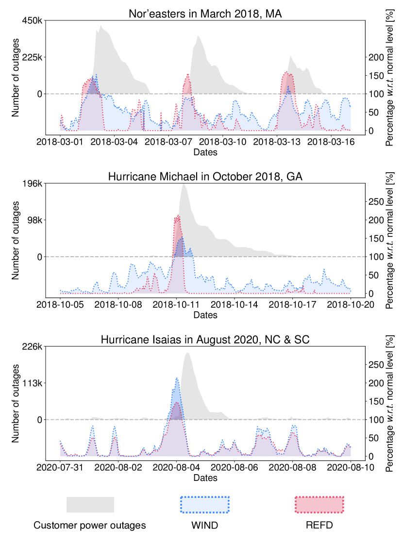
(a)

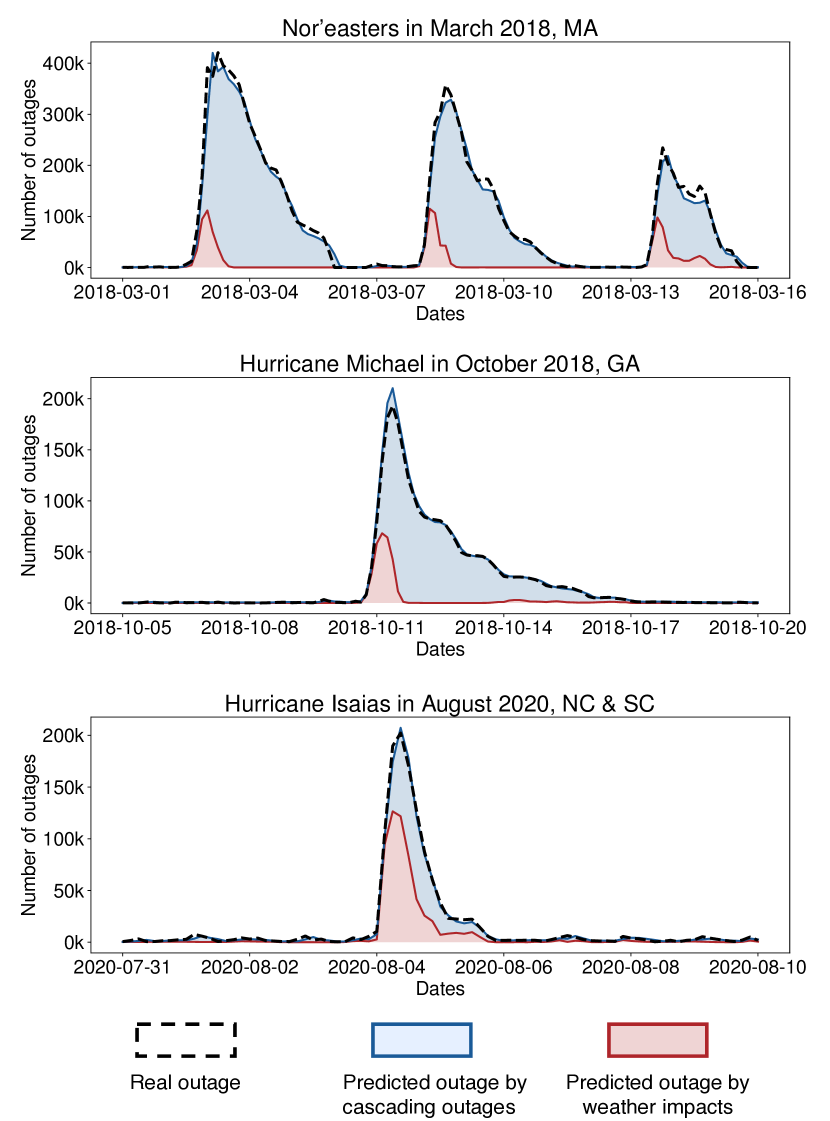
(b)

Figure 5: Spatially aggregated power outage and weather effect. (a) Spatially aggregated totals of customer outages per minute and the corresponding two leading weather factors compared to their maximum normal levels. The left vertical coordinate corresponds to the total number of customer outages per minute reported in the entire service territory, and the right vertical coordinate corresponds to the relative percentage of the weather data with respect to its three-sigma limits in the daily operation. (b) Total number of customer outages and corresponding decoupling according to our model estimation. Blue and red regions represent the estimated number of outages caused by cascading outages and the number of outages directly caused by extreme weather, respectively. Black dashed lines represent the true total number of customer outages.

Spatio-temporal model for customer power outages

Next, we modeled the number of outages without access to detailed disruption and restoration records. It should be noted that outage occurrence and system restoration can and do occur simultaneously, and the two opposite movements constitute the overall power outage evolution process. Therefore, modeling these two dynamics separately is not practical. Rather than modeling the physical process, we built a spatio-temporal model (see Methods) from customer power outages and weather data in which the number of outages in each geographical unit is regarded as a non-homogeneous Poisson process, and these processes interact with each other in an underlying topological space determined by distance and possible grid connectivity. The distribution of customer power outages in a geographical unit at any given time is specified by an occurrence rate of customer power outage (referred to as “outage occurrence rate”in the rest of this paper). To simulate customer outages in a power system in severe weather conditions, we assume that (1) the outage occurrence rate of a unit affected by extreme weather will grow as the cumulative weather effect builds until it reaches the system’s minimal functionality, (2) a unit with a larger number of customer power outages has a better chance of raising the outage occurrence rate in its neighboring units (in the topological space) due to the potential damage to the large transmission network serving these units, and (3) the outage occurrence rate of a unit will also decline exponentially over time as the restoration plan is followed throughout the region.

We fitted the model using real data and evaluated its predictive performance. The results show that our model achieves promising accuracy in terms of predicting the number of customer power outages in a given unit three hours in advance. Figure 5 gives an example of in-sample prediction (indicated by blue and red regions combined) using our model for three service territories during different weather events. This example evaluates the model’s predictive capabilities, using observed data, to see how effective the model is in reproducing the data. Our model achieves promising results compared to the ground truth, indicated by black dashed lines, and it reveals that the direct impact of cumulative extreme weather (red area) causes only a relatively small number of customer power outages in some local regions. It is with indirect damage (the blue area) rippling through the entire region that a large-scale customer power outage starts to emerge. We also apply the methodology outlined above to daily operations and achieve a similar predictive accuracy, indicating that the grid resilience captured by our model is inherent in power distribution infrastructure and operations. More numerical results can be found in the Supplementary Material.

4 Descriptive analysis of extreme weather effect

Next, we studied the impact of the cumulative weather effect by analytically evaluating the relationship of the outage ratio to the cumulative weather effect in each geographical unit in which the decay rates in the proposed model can be learned from the data. Here we selected three representative weather variables to demonstrate such relationships: composite radar reflectivity (REFC), derived radar reflectivity (REFD), and wind speed (WIND). These features describe the intensity of precipitation and wind, which are among the most important factors in weather-induced outages. We calculated the accumulation of these features for the preceeding three days at every time point during three extreme weather incidents. Strikingly, the outage ratio stays close to zero until the cumulative weather variable reaches a certain threshold, where a sharp jump occurs (indicated by blue lines) as shown in Figure 6. Such a trait can be captured well by a sigmoid function with the value of the cumulative weather effect. These “thresholds” have a strong correlation to the DTC of the system for the corresponding weather variable.

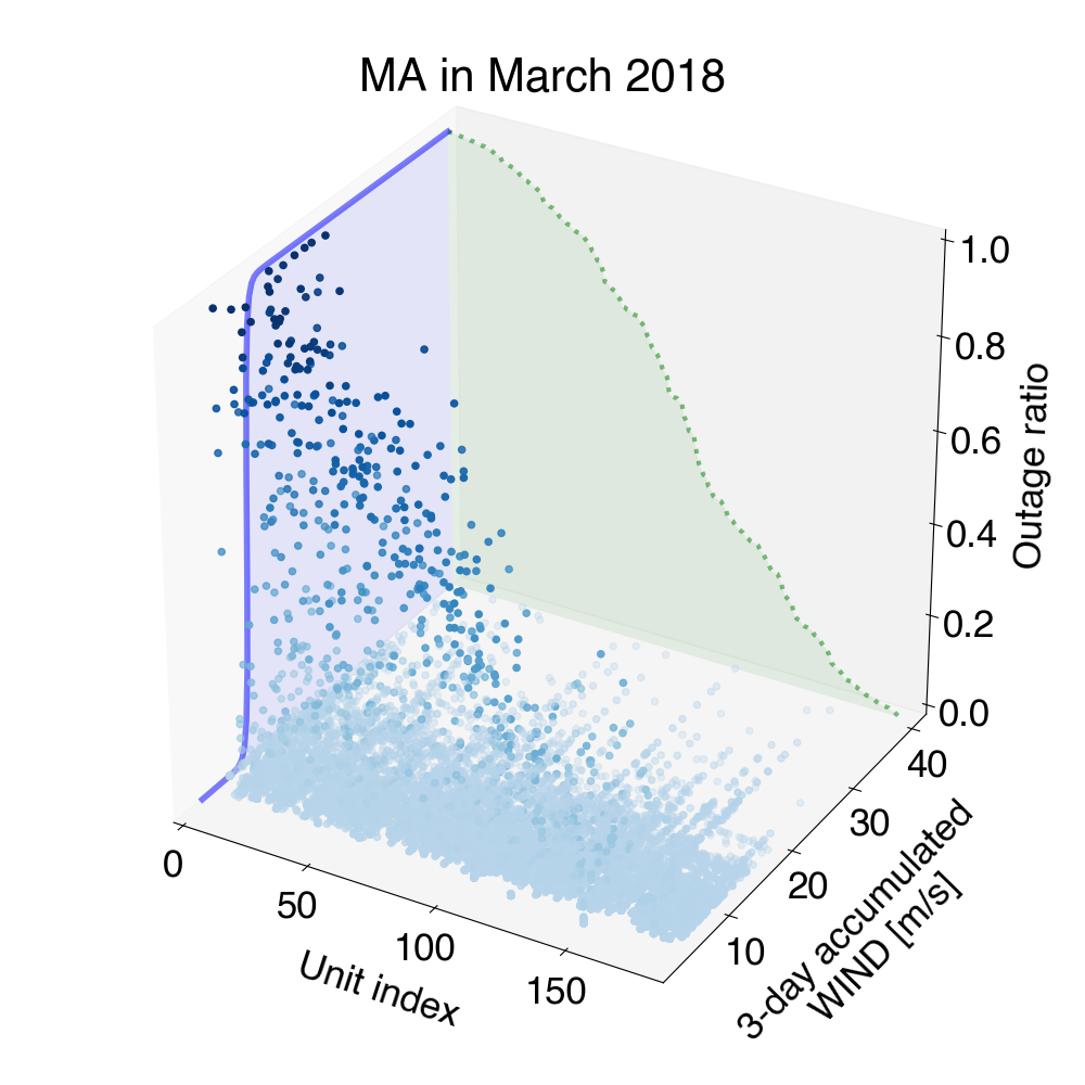
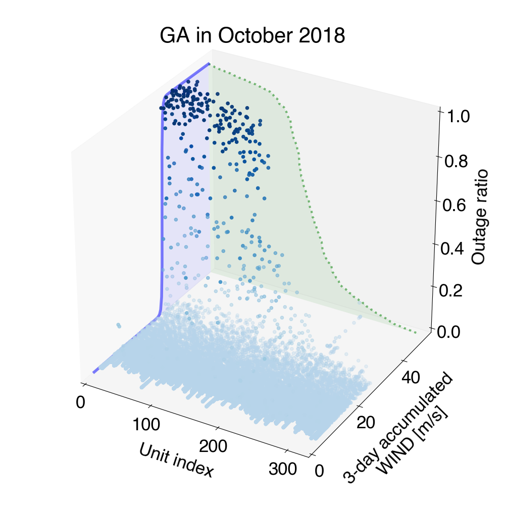
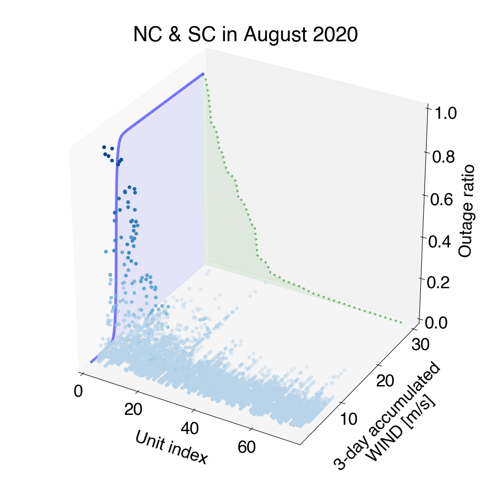
Figure 6: Cumulative weather effect versus outage ratio during the degradation stage. Scatter plots of outage ratios as the number of outages declines, given the accumulation of three different types of weather effects. The vertical and left horizontal coordinates are the outage ratio and geographic unit, respectively. Each data point corresponds to the outage ratio (total number of customer outages/total number of customers) of a certain unit at a certain time. The color depth of the data points also indicates the outage ratio. The unit IDs have been sorted by their historical maximum outage ratios in descending order. The right horizontal coordinate is the corresponding cumulative weather effect for the preceeding three days. The blue line on the left vertical plane is a sigmoid curve fitted by all the data points with an outage ratio larger than 0. The green dotted line on the right vertical plane is the maximum outage ratios of all units.

The result reveals that a power grid has a DTC within which it can easily withstand external impacts without substantial outages. Systems with larger capacities are more resilient to weather effects (i.e., more cumulative weather effect is needed to initiate large-scale power outages). The prevalence of this phenomenon in the three major service territories confirms the existence of infrastructure resistance. For example, in Figure 6, we can observe that the DTC for wind speed in Massachusetts, North Carolina, and South Carolina (around 10 m/s) is much smaller than that of Georgia (around 30 m/s). This implies that the power systems in Massachusetts, North Carolina and South Carolina are more resilient to strong wind than the system in Georgia. We also find that there is a considerable difference in the distribution of maximum outage ratios (indicated by green shaded area) among three service territories, and the maximum outage ratio is negatively related to its DTC. For example, extreme weather is devastating to nearly half of the geographic units (296) in Georgia as the maximum outage ratio for these units approaches 1 ($>0.95$), while the other units are barely affected by the severe weather events (the maximum outage ratio stays around 0). As opposed to the half-and-half phenomenon in Georgia, the outage ratio for the majority of the units in North Carolina and South Carolina remains remarkably low throughout the weather events. We note that the outages in North Carolina and South Carolina are most likely due to damaged distribution network infrastructure, which is spread out and has lower shared impacts. In other words, the transmission network infrastructure in these states performs better in terms of withstanding extreme weather events than that in Georgia. This could be partly due to the fact that the transmission line structures in North Carolina and South Carolina are required to withstand wind speeds of 45 m/s or more (per the National Electric Safety Code) as they are installed close to the coast and potentially in the path of hurricanes.

5 Resilience quantification

Resilience can be described in two ways: infrastructure resistance and operational recoverability, which correspond to the responses of the system facing external impacts and restoration tasks, respectively [24], as shown in Figure 1 (a). Infrastructure resistance refers to the inherent ability of the power grid to anticipate, resist, and absorb the effects of hazardous events, and determines a system’s DTC. Operational recoverability refers to the system’s ability to recover from damage inflicted by extreme weather through a series of operational measures adopted by system operators, utility companies, and other support entities. To be specific, infrastructure resistance in our model can be described by the relationship between the cumulative weather effect and the power system functionality (number of remaining customers with power), and operational recoverability can be defined as the speed of a unit’s recovery from a power outage, as described by the outage occurrence rate.

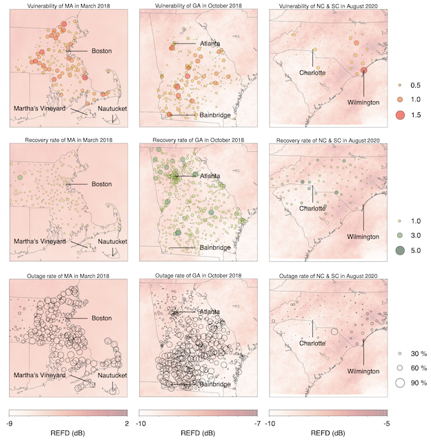
Figure 7: Design margin and operational recoverability. Bubble sizes in each row from top to bottom represent design margin insufficiency (vulnerability), recovery rate, and outage ratio of units during studied events, respectively. The value of design margin insufficiency represents the average number of outages occurring in the given unit produced by a unit of cumulative weather effect. The number of outages in each geographic unit declines exponentially (the exponential rate is specified by the recovery rate). The depth of color in the background indicates the average weather intensity (REFD) during corresponding events.

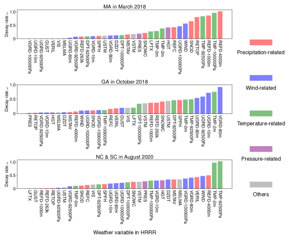
Figure 8: Decay rate in accumulating weather effect. Bars represent the learned decay rate $\omega$ for each weather variable in the corresponding service territories, where colors indicate their categories. The weather variables have been sorted by their values.

Infrastructural resistance

Our model suggests that there are three factors affecting power systems’ infrastructure resistance: design margin sufficiency, maintenance sufficiency, and topological criticality (Figure 1 (b)).

Design margin is a consideration of higher physical design standards, which can improve the power infrastructure’s resistance to extreme weather events. Such designs include (but not limited to) using steel structures (instead of wood ones), increasing diameters of poles, elevating power lines (to minimize risk of tree-contact faults), installing concrete foundations (to strengthen the footing of a structure), using high-strength/light-weight overhead conductors (to minimize conductor sag), and converting overhead conductors to underground cables. Note that increasing design margin typically results in a higher cost, which enforces electric utilities to consider such trade-off and make corresponding decisions (resilience versus economy). In our model, we introduce a set of trainable parameters for each geographic unit representing its overall design margin sufficiency (or vulnerability) to extreme weather, where the coefficient value represents the number of outages occurred in this unit caused by a unit of cumulative weather effect. A larger coefficient indicates that the corresponding geographical unit is more vulnerable to extreme weather and more likely to suffer a massive blackout when the extreme weather effect excessively accumulates (Figure 7). It can be observed in the top row of Figure 7 that the vulnerability indices for metropolitan areas (e.g., Boston, Atlanta, and Charlotte) are relatively low, which is most likely because the vegetation in well-developed areas is less dense and therefore, easier to maintain and less likely to cause faults (e.g., a tree falling on a power line).

The power industry regularly inspects and maintains electrical components and facilities to sustain the health of its infrastructure. Our second factor, power grid maintenance, refers not just to the maintenance of assets and equipment but also to the environment in the vicinity, e.g., vegetation inspection and trimming. Insufficient maintenance may leave the system vulnerable to the impact of extreme weather and exacerbate existing vulnerabilities [23]. This factor can be captured by the rates defined in the cumulative weather effect: The smaller the rate a unit has, the less maintenance has been completed and the faster weather effects will accumulate (Figure 8).

Our third factor, topological criticality, refers to the fact that some components or facilities are critical to the resilience of a power system. Modern power grids are interdependent networked systems [10, 28, 29, 41, 44], and the failure of some critical portions might affect not only customers’ power within their own service territories but could also degrade the entire system’s resistance ability and lead to the failure of other dependent nodes in the same networks via the common mechanism of cascading failures and blackouts. Note that we consider each geographic unit in the power network to be a node, and we model connectivity between nodes using a directed graph [49] in which directed edges between nodes represent the direction of a power outage’s propagation. The weight of each edge indicates the average number of outages in the target unit that results from an outage in the source unit. Because we assumed that an increase in the number of power outages in a geographical unit can lead to a proportional increase (determined by the edge value between two connected nodes) in the number of power outages in the unit it connects to, the criticality of a unit can be precisely evaluated by the total number of customer power outages in other directly connected units that result from its failure. Our results show that disruptions in only a small number of critical geographic units can lead to a large-scale subsequent customer power outages in all three service territories (see the units with major outgoing links in Figure 9). This indicates that these units are critical in the evolution of power outages: A major portion of the power outages can be directly or indirectly attributed to these units. This characteristic is important because it shows some weak points in the resilience of the grid, and the utility needs to concentrate resources on enhancing these critical units. In addition, we can observe in Figure 9 that the most frequent sources of outage propagation are the mid-size urban areas (e.g., Barnstable, MA, Macon, GA, and Wilmington, NC) instead of large cities (e.g., Boston, Atlanta, and Charlotte) or rural areas. As a result, we can conclude that an area that is not a dominant load center (i.e., metropolitan area) but interconnects with multiple transmission facilities or hosts a large generation capacity is more likely to be a power outage propagation source.

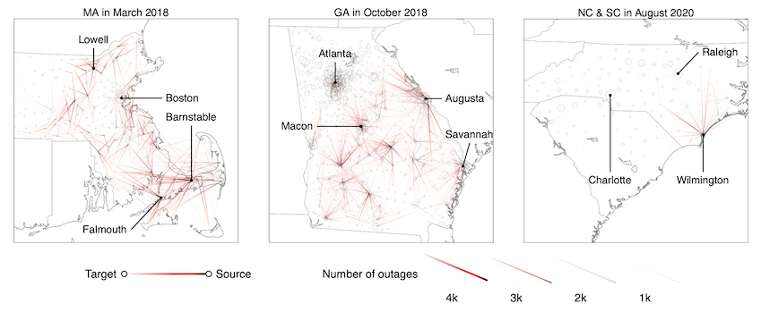
Figure 9: Power outages propagation map. The map shows the spatial propagation of power outages among geographical units during extreme weather. An edge between two units indicates that the power outages that occur in one unit (light red) are the result of an outage in the other (dark red). Edge width and color depth represent the number of customer power outages at the target attributed to the source. The size of dots represents the total number of customers of the corresponding geographical unit.

Recoverability

We now turn our attention to the operational recoverability of power systems. We assume that the recovery process in each geographic unit reduces the number of outages at an exponential rate, which is captured by another set of parameters that may vary from unit to unit. At a high level, 92% of customer power outages are over within 6 hours, and all customers are back to normal within one day, as shown in Figure 4. However, recoveries from damage caused by extreme weather lasted 4, 4, and 2 days for the three service territories, and geographic units in different regions may also carry out their restoration activities differently. Differences in restoration processes may stem from various factors, including infrastructure damage severity, restoration plan efficacy, resources (human, funding and supplies), and the coordination of restoration progress [34]. For example, six months after Hurricane Maria hit Puerto Rico, more than 10 percent of the island’s residents were still without power [3]. Similarly, it took the U.S. Virgin Islands more than four months to fully restore power after being hit by Hurricanes Irma and Maria. Recovery in the U.S. mainland has been much quicker—in part because the resources are more abundant. In particular, after Irma hit the southeast U.S., knocking out power to 7.8 million customers, 60,000 utility workers from across the country were deployed and restored power to 97 percent of the population in about a week [33].

According to the fitted model, the recovery rates for urban areas are usually higher than those for rural areas because it is easier to find repair personnel, identify fault locations, and access and repair a fault that occurs in an urban area. Rural areas tend to lack resources and include terrain that is challenging for repair personnel to access and manage (e.g., mountains, rivers, forests). This explains why the recovery rates for the Atlanta area are relatively high. As a result of lower vulnerability and higher recoverability, the outage rates for metropolitan areas (e.g., Boston, Atlanta, and Charlotte) should be relatively low, and this is verified by the outage rate maps on the bottom row of Figure 7.

6 Resilience enhancement analysis

Many previous efforts [1, 24, 27, 30, 32, 34, 35, 47] have assessed a variety of techniques that can be employed before an event occurs in an effort to enhance system resilience: (1) improving system architectures to further reduce the criticality of individual geographic units in the power network, (2) enhancing the health and reliability of individual geographic units, (3) making restoration plans before events occur to speed up help to those who may need it, and (4) monitoring asset health and employing preventive- and reliability-centered maintenance. However, examining and evaluating the effectiveness of resilience enhancement strategies could be technically intractable, for a number of reasons: First, due to the low frequency of extreme weather events, there is a lack of weather data and corresponding power outage records for such an evaluation. Second, the uniqueness of each extreme weather event and its ripple effects makes the reproducibility of large-scale outages in resilience studies difficult. And third, an accurate evaluation of these strategies requires a partnership across all levels of government and the private sector, which is too time-consuming and costly to be carried out in practical terms.

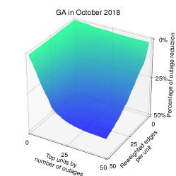
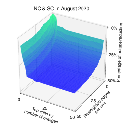
(a)

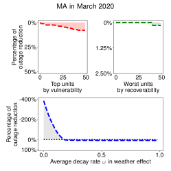
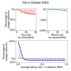
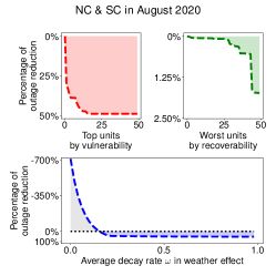
(b)

Figure 10: Resilience enhancement simulation results. (a) Outage reduction from re-weighting the edges with the largest weights in the network to the average level. The left horizontal coordinate represents the number of top geographic units (by maximum number of outages) that we want to improve during extreme weather incidents. The right horizontal coordinate represents the number of edges per unit we need to re-weight, and the vertical coordinate represents the simulated corresponding percentage of outage reduction compared to the real number. (b) The outage reduction from re-weighting the geographic units with the highest design margin insufficiency and lowest recoverability coefficients to their average levels. The left and right horizontal coordinates represent the number of units with the largest design margin insufficiency and smallest recoverability coefficients, respectively, that we want to improve during extreme weather incidents, and the vertical coordinate represents the corresponding percentage of outage reduction compared to the real number.

We can now identify and evaluate strategies in four general areas—design margin, recoverability, criticality, and maintenance) that, if adopted, could significantly increase power grid resilience. Even though these strategies cannot be reliably and accurately assessed in the absence of detailed failure and restoration records, our model still offers the opportunity to simulate the entire process of large-scale customer power outages in different circumstances and explore potential opportunities to help alleviate the effects of extreme weather. Specifically, we “improve” certain aspects of power grid resilience by adjusting the corresponding parameters of the fitted model, then simulate an outage process in a given weather condition, and finally calculate the outage reduction rate compared to the original number of outages (Figure 10). We observe that de-escalating the criticality of the small number of units with the most customer power outages can effectively mitigate the ultimate impact of extreme weather. For example, in Massachusetts, re-weighting the largest 50 edges of the top 10 geographic units, such as Boston and Cambridge, by their number of customer power outages, can reduce customer power outages by 47.8%. In Georgia, the same strategy can reduce customer power outages by 38.4%. However, the same strategy may not achieve the same results in North Carolina and South Carolina. Instead, improving design margin for a geographic unit with a large number of customer power outages, i.e., Wilmington, can reduce the total number of outages by 32%. Outages can be reduced further—by 49.8%—if the top 12 units are given the same treatment. We also notice that improving the rate of maintenance is not as rewarding as other strategies; however, the system will degrade if the maintenance rate drops below the current level. This is because maintenance is already well-managed by local operators.

7 Discussion

To summarize what we have found in using our grid resilience model: (1) Outage rates in metropolitan or economically strong areas are generally lower, due to less vegetation, more underground or steel-structure-supported power lines, and adequate repair resources. In other words, the electricity infrastructure in those areas is less vulnerable to extreme weather events and more recoverable if damage to infrastructure occurs. (2) On the other hand, rural areas, especially those with more difficult terrain, such as mountains, forests, rivers, and deserts, are hard to access and make it challenging to locate a fault, which inevitably delays an outage recovery. In addition, those economically weaker areas may lack the budget to maintain or upgrade their electricity infrastructure, which becomes increasingly vulnerable to extreme weather events. As a result, rural areas typically have relatively high outage rates. (3) The direction (source to target) of outage propagation typically follows the power flow direction. In other words, an area with a large generation capacity or dense transmission network facilities (e.g., substations) is probably a hub of outage propagation. Such an area is more likely to be a mid-size urban area developed to host a number of transmission or generation facilities and is usually not a big load center that dominates power flows.

Planning and operational measures to prevent and mitigate weather-induced power outages can be derived from our quantitative analysis and simulated resilience enhancement. The first observation is that the power grid shows some vulnerability to major outage propagation, which significantly exacerbates the initial impact of weather events. If such outage evolution and propagation can be prevented or mitigated, the weather impact could be much smaller and more easily contained. A key to stemming outage propagation is to reduce interdependence when facing outage risks. The interdependency of power grids is closely related to their interconnected nature, and it is neither economical nor practical to simply break power grids into local pieces. A more desirable way to reduce the risks of major outages exacerbated by interdependence is to improve the operational flexibility of the power grid. A flexible power grid should embrace diversified sources with distributed locations and versatile operation schemes. For example, distributed energy resources (DER) can provide energy to local loads and thus reduce the risk of outages caused by interruption of distant electricity transmission. Energy storage can also quickly supply energy to local or nearby loads. Moreover, microgrids characterized as local power grids with diverse energy sources and flexible operation modes can easily connect to or isolate from the main power grid, which is resilient to external threats and sustainable.

Methods

Data

This paper studies power grid resilience to extreme weather by taking advantage of a unique set of fine-grained customer-level power outage records and comprehensive weather data. The data cover three major service territories across four states on the east coast of the United States, including Massachusetts, Georgia, North Carolina, and South Carolina, spanning more than 155,000 square miles, with an estimated population of more than 33 million people in 2019. The extreme weather events we studied in this paper include winter storms in Massachusetts (MA) in March 2018, Hurricane Michael in Georgia (GA) in October 2018, and Hurricane Isaias in North Carolina (NC) and South Carolina (SC) in August 2020.

Customer power outage data in this work were collected by web crawlers from the Massachusetts state government [2], Georgia Power [42], and Duke Energy [17] web sites, respectively, between December 31, 2017 through August 31, 2020. The data record the number of customers without power in each geographical unit at 15-minute intervals. These service territories are divided into hundreds of geographical units defined by township, zip code, or county. There are 351 units and 2,755,111 customers in Massachusetts, 665 units and 2,571,603 customers in Georgia, and 115 units and 4,305,995 customers in North Carolina and South Carolina. See a summary of the outage data in Supplementary Table 1 for more details. The HRRR model [8] is a National Oceanic and Atmospheric Administration (NOAA) real-time, 3 km resolution, hourly updated, cloud-resolving, convection-allowing atmospheric model, initialized by 3 km grids with 3 km radar assimilation. Radar data is assimilated into the HRRR model every 15 minutes over a 1 hour period, adding further detail to that provided by the hourly data assimilation from the 13 km radar-enhanced rapid refresh. In this work, we selected 34 variables in the HRRR model (Supplementary Table 2) that characterize near-surface atmospheric activities directly linked to weather impacts on power grids. To match the spatial resolution with the customer power outage data, we aggregated the regional weather data in the same geographic unit by taking the average. To reduce noise in both the outage data and the weather data, we also aggregated the number of customer power outages and the value of weather variables in each unit into three-hour time slots.

We studied three typical extreme weather events between 2018 and 2020 during which customers in these three service territories were significantly affected and for which the number of outages, as well as weather information for each geographical unit, was included in our data set. These three events are as follows. March 2018 nor’easters: The March 2018 nor’easters included three powerful winter storms in March 2018 that caused major impacts in the northeastern, mid-Atlantic and southeastern United States. At its peak, more than 14% of the customers (385,744) in Massachusetts remained without power, and outage ratios for nearly 30% of the geographic units in the region (104) were over 50%. Hurricane Michael: Hurricane Michael was a very powerful and destructive tropical cyclone in October 2018 that became the first Category 5 hurricane to strike the contiguous United States since Andrew in 1992. About 7.5% of the customers (193,018) in Georgia were severely affected by the storm and lost power, and the outage rates for about 25% of the geographic units in Georgia (166) were above 50%. Hurricane Isaias. Hurricane Isaias was a destructive Category 1 hurricane in August 2020 that caused extensive damage across the Caribbean and the U.S. east coast and included a large tornado outbreak. At its peak, about 13% of the customers in North and South Carolina lost power, and the outage ratios for nearly 9% of the geographic units in these two states were above 50%. For the three service territories, we determined the study periods based on power outage records and the associated weather data, including derived radar reflectivity, composite radar reflectivity, and wind speed. As a result, March 1 to March 16, 2018 is considered to be the period of the March 2018 nor’easters for service territories in Massachusetts, October 5 to October 20, 2018 the period of Hurricane Michael for service territories in Georgia, and August 1 to August 10, 2020 the period of Hurricane Isaias for service territories in North Carolina and South Carolina. To fairly compare resilience differences in the same conditions, for each event we considered daily operations in the rest of the relevant month, without the impact of extreme weather, to be the baseline (Supplementary Table 1).

Spatio-temporal non-homogeneous Poisson process.

We presented a data-driven spatio-temporal model for the number of customer power outages that also captures the spatio-temporal dynamics of customer power outages across the region. We first defined the cumulative weather effect, then we proposed a non-homogeneous multivariate Poisson process for the number of customer power outages across the service territory:

Assume there are $K$ geographical units in the service territory and $T$ time slots in the time horizon that spans the entire event. We also consider $M$ different weather variables. Let $i,j\in\{1,\dots,K\}$ denote the index of units, $t\in\{1,\dots,T\}$ denote the index of time slots, and $m\in\{1,\dots,M\}$ denote the index of weather variables. Let $N_{it}\in\mathbb{Z}_{+}$ be the number of customer power outages we observed in unit $i$ at time $t$ and let $x_{i,t,m}\in\mathbb{R}$ be the value of weather variable $m$ in unit $i$ at time $t$ recorded by weather data.

We defined the cumulative weather effect as a discounted sum of recent weather influences. Formally, for a weather variable $m$, the accumulation of weather effect $v_{i,t,m}$ in unit $i$ at time $t$ is written as follows:

$$v_{i,t,m}=\sum_{\tau=t-d+1}^{t}x_{i,\tau,m}\exp\{-\omega_{m}(t-\tau)\},$$

where $d$ denotes the time window, $x_{i,\tau,m}$ is the value of weather variable $m$ in unit $i$ at time $\tau$, and $\omega_{m}\geq 0$ is a learnable rate for weather variable $m$. The larger $\omega_{m}$ is, the faster the weather effect decays. The weather effect does not fade away if $\omega_{m}=0$.

The distribution of customer power outages in a unit at any given time is specified by an occurrence rate of customer power outage, or more simply, outage occurrence rate. To be specific, we model the outage occurrence rate in each unit and at arbitrary time as a Poisson process, i.e., $N_{it}\sim\text{Poisson}(\lambda_{it})$, where the outage occurrence rate in unit $i$ at time $t$ can be characterized by $\lambda_{it}$. We denote the accumulation of all weather variables in unit $i$ at time $t$ as a vector $\boldsymbol{v}_{it}=[v_{i,t,1},v_{i,t,2},\dots,v_{1,t,M}]^{\top}\in\mathbb{R}^{M}$. We define the power network in the service territory as a directed graph $\mathcal{G}=(\mathcal{V},\mathcal{E})$, where $\mathcal{V}=\{i:1\leq i\leq K\}$ is a set of vertices representing the units, and $\mathcal{E}\subseteq\{(i,j):i,j\in\mathcal{V}^{2}\}$ is a set of directed edges (ordered pairs of vertices) that represents underlying connections between units. As we assumed that customer power outages can be produced by either the direct impact of the cumulative weather effect or the indirect impact of outages in the connected units, we defined the outage occurrence rate as the following:

$$\lambda_{it}=\underbrace{\vrule width=0.0pt,height=0.0pt,depth=14.63881pt\gamma_{i}\mu(\boldsymbol{v}_{it};\varphi)}_{\begin{subarray}{c}\text{direct impact}\\ \text{induced by weather}\end{subarray}}+\underbrace{\vrule width=0.0pt,height=0.0pt,depth=8.61108pt\sum_{t^{\prime}<t}\sum_{(i,j)\in\mathcal{E}}g(i,j,t,t^{\prime})}_{\begin{subarray}{c}\text{indirect impact}\\ \text{from connected units}\end{subarray}},$$

where $\gamma_{i}\geq 0$ is the design margin of unit $i$. Function $\mu(\cdot;\varphi)\geq 0$ returns the weather-induced outage occurrence rate, approximated by a deep neural network parametrized by $\varphi$ given the cumulative weather effect in the past as input. The architecture of the neural network is described in Supplementary Figure 3. Function $g(i,j,t,t^{\prime})\geq 0$ is the triggering effect on unit $i$ at time $t$ from previous outages occurred in unit $j$ at time $t^{\prime}$. There are many possible forms of function $g$. Here we adopt one of the most commonly used forms, which assumes the triggering effect of decay exponentially over time [43]:

$$g(i,j,t,t^{\prime})=\alpha_{ij}N_{jt^{\prime}}\beta_{j}e^{-\beta_{j}(t-t^{\prime})},~{}\text{for}~{}(i,j)\in\mathcal{E}~{}\text{and}~{}t>t^{\prime},$$

where $\beta_{j}\geq 0$ captures the rate of the influence. Note that the kernel function integrates to 1 over $t$. We assumed that each edge $(i,j)\in\mathcal{E}$ is associated with a non-negative weight $\alpha_{ij}\geq 0$ indicating the correlation between unit $i$ and $j$. The larger the weight $\alpha_{ij}$, the more likely it is the unit $i$ will be influenced by unit $j$. We also assume $\alpha_{ii}=1,$ and $~{}i\in\mathcal{V}$, so $\beta_{j}$ can be regarded as the recovery rate of unit $j$. In particular, $g(i,i,\cdot,\cdot),~{}i\in\mathcal{V}$ captures the dynamics of the restoration process of unit $i,$ and $g(i,j,\cdot,\cdot),~{}i,j\in\mathcal{V},~{}i\neq j$ captures the influence of unit $j$ on unit $i$. We also disallow the presence of loops between two arbitrary units, i.e., $\alpha_{ij}=0$ if $\alpha_{ji}\neq 0$.

The model can be estimated by maximizing the log-likelihood of the parameters, which can be solved by stochastic gradient descent [26]. Denote the set of all the parameters $\{\alpha_{ij}\}_{(i,j)\in\mathcal{E},i\neq j}$, $\{\beta_{i}\}_{i\in\mathcal{V}}$, $\{\gamma_{i}\}_{i\in\mathcal{V}}$, $\{\omega_{i}\}_{i\in\mathcal{V}}$, and $\varphi$ as $\theta$. Denote the corresponding parameter space as $\Theta=\mathbb{R}_{+}^{K\times K}\times\mathbb{R}_{+}^{K}\times\mathbb{R}_{+}^{K}\times\mathbb{R}_{+}^{K}\times\Phi$, where $\Phi$ is the parameter space of the neural network defined in $\mu$. Denote all the observed customer power outages and weather data in the studied service territory and time horizon as $N=\{N_{it}\}_{1\leq i\leq K,1\leq t\leq T}$ and $X=\{x_{i,t,m}\}_{1\leq i\leq K,1\leq t\leq T,1\leq m\leq M}$. Our objective is to find the optimal $\hat{\theta}$ by solving the following optimization problem:

$$\underset{\theta\in\Theta}{\mbox{maximize}} \quad\ell(\theta|N,X)\coloneqq-\sum_{t=1}^{T}\sum_{i=1}^{K}\lambda_{it}(\theta)+N_{it}\log\left(\lambda_{it}(\theta)\right)$$

subject to $$\quad\alpha_{ii}=1,~{}\quad\forall i\in\{1,\dots,K\},$$

where $\ell$ denotes the log-likelihood function.

Supplementary Material

Supplementary Note 1

Several examples of in-sample prediction at the unit level are shown in Supplementary Figure 1. The results show good performance in recovering the outage evolution for units with various number of customers, which further confirms that our model attains a robust explanatory power on real data.

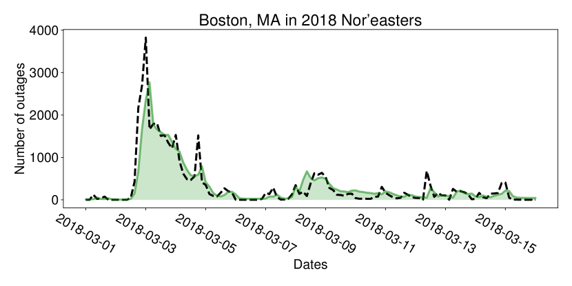
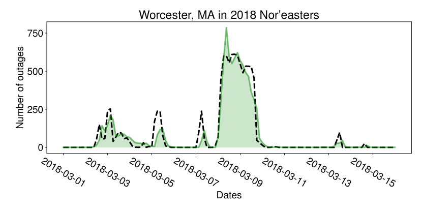
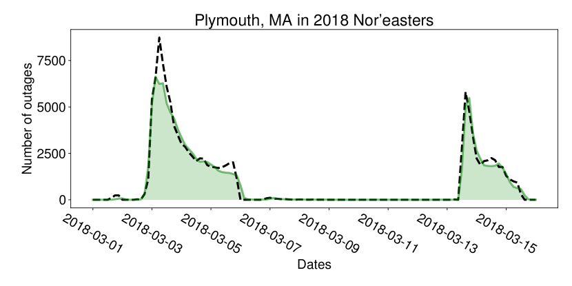
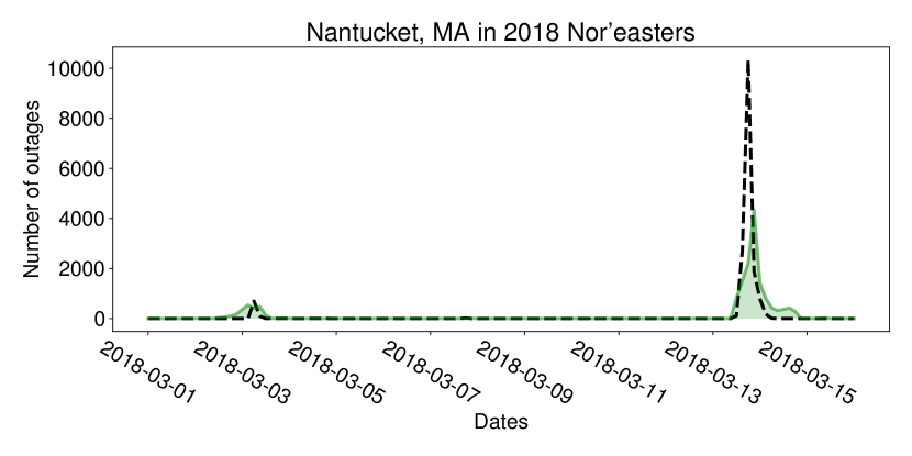
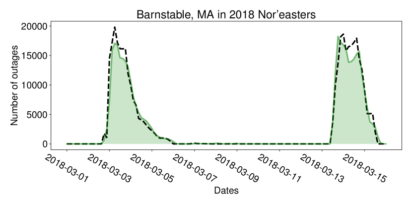
(a) March 2018 nor’easters

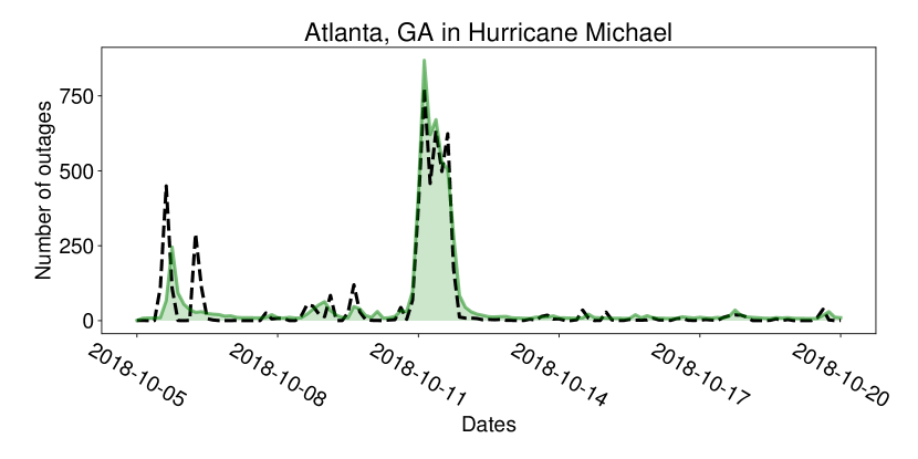
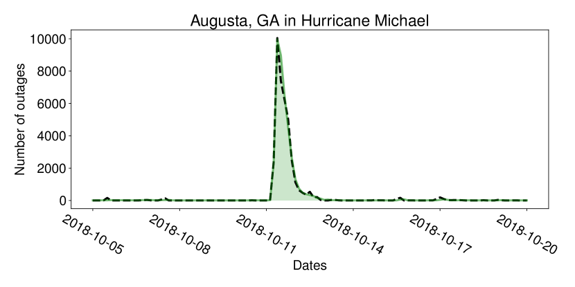
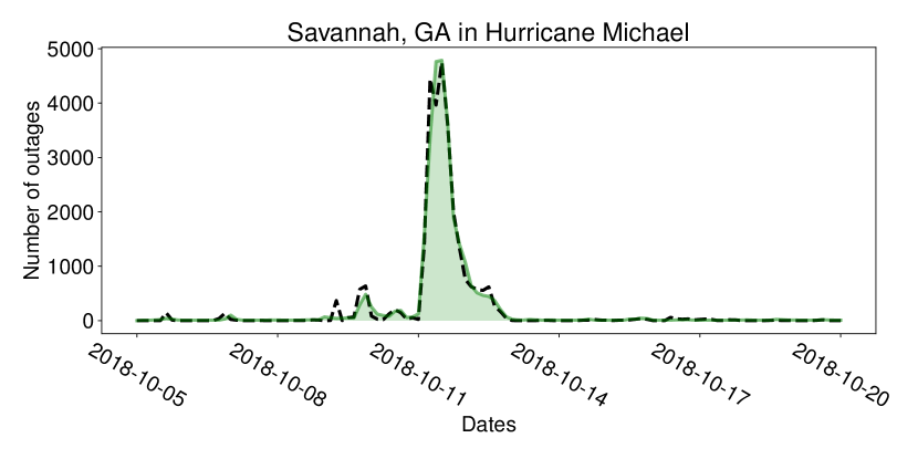
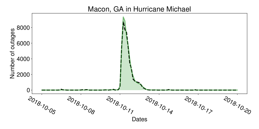
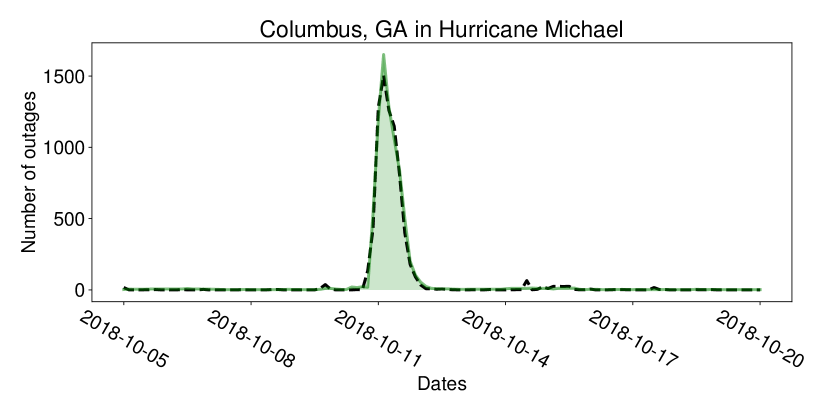
(b) Hurricane Michael

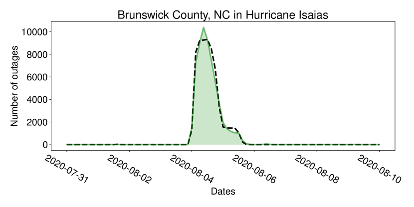
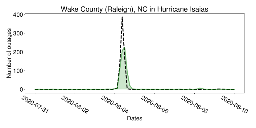
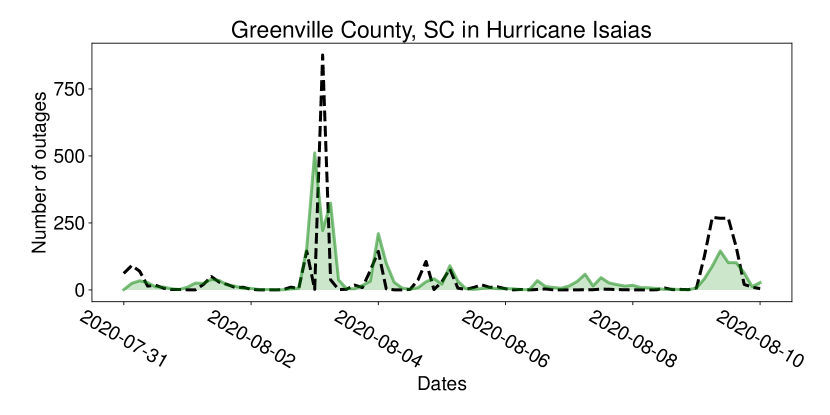
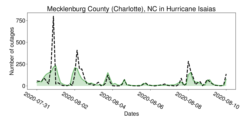
(c) Hurricane Isaias

Supplementary Figure 1: Unit-level predictions units in (a) Massachusetts (March 2018 nor’easters), (b) Georgia (Hurricane Michael), and (c) North Carolina and South Carolina (Hurricane Isaias). Black lines represent the real customer power outages in the certain area and green shaded regions represent the in-sample prediction for customer power outages in the same area using our model.

In addition to the in-sample estimation, we also fitted the model using real data and evaluated its performance on one-step-ahead (out-of-sample) prediction. The prediction procedure withholds the future data from the model estimation, then uses the fitted model to make predictions for the (held-out) data at the next time slot. Here we collect the customer outage data and the corresponding weather data for another seven extreme weather events: three hurricanes (Dorian, Hanna, Laura) and four tropical storms (Alberto, Gordon, Imelda, Beta). For the same region, we took the data of several events in the past as the training set to fit the model and then tested its predictive performance on another event in the future. The results in Supplementary Figure 2 show that our model achieves promising accuracy in unit-level prediction for the number of customer power outages three hours ahead.

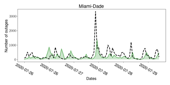
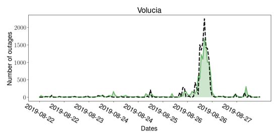
(a) Hurricane Isaias

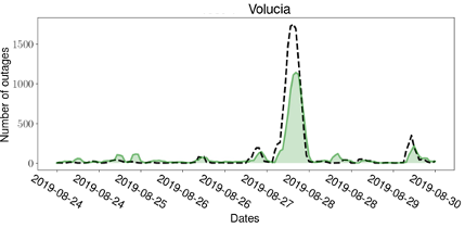
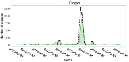
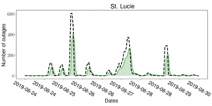
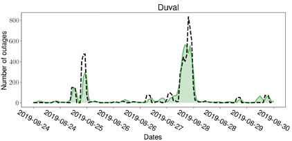
(b) Hurricane Dorian

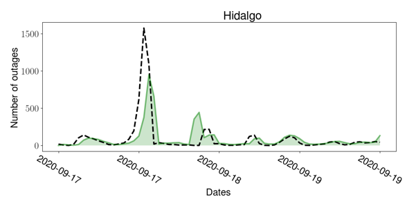
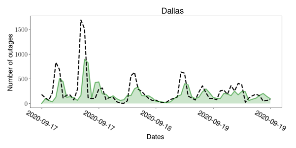
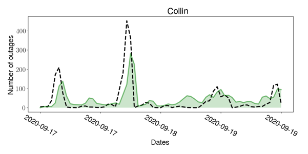
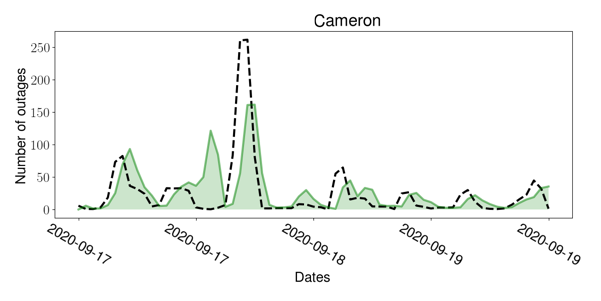
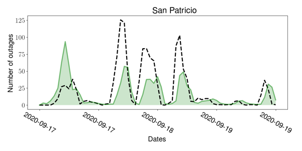
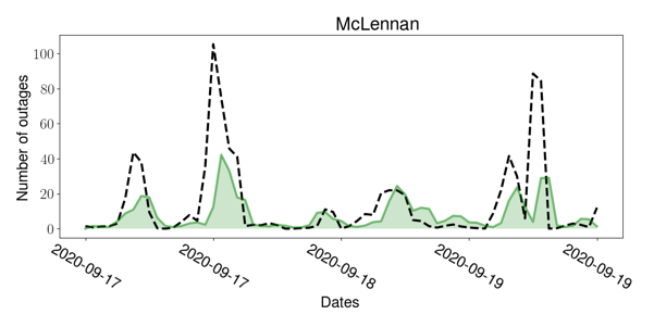
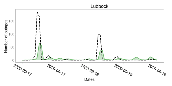
(c) Tropical Storm Beta

Supplementary Figure 2: Three unit-level out-of-sample prediction results: (a) Training set: Hurricane Dorian (08-24-2019 to 09-07-2019). Testing set: Hurricane Isaias (07-30-2020 to 08-04-2020). (b) Training set: Tropical Storm Alberto (05-25-2018 to 06-02-2018), Tropical Storm Gordon (09-03-2018 to 09-11-2018), Hurricane Michael (10-07-2018 to 10-17-2018). Testing set: Hurricane Dorian (08-24-2019 to 09-11-2019). (c) Training set: Tropical Storm Imelda (09-17-2019 to 09-20-2019), Hurricane Hanna (07-23-2020 to 07-27-2020), Hurricane Laura (08-20-2020 to 08-30-2020). Testing set: Tropical Storm Beta (09-17-2020 to 09-25-2020). Black lines represent the real customer power outages, and green shaded regions represent the three-hour-ahead prediction for customer power outages in the same area using our model.

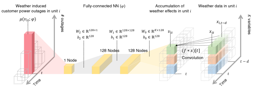
Supplementary Figure 3: Architecture of the neural network.

Supplementary Table 1: Customer power outage data sets used in this study.

	Basic information				Extreme weather event				Daily operation
	Units	Unit type	Customers		Time period	Average outages	Max outages		Time period	Average outages	Max outages
MA	351	township	2,755,111		03-01-2018—03-15-2018	2393	19964		03-16-2018—03-31-2018	49	1096
GA	665	zipcode	2,571,603		10-05-2018—10-20-2018	359	7182		10-21-2018—11-05-2018	38	1659
NC & SC	115	county	4,305,995		07-31-2020—08-10-2020	2198	92424		08-11-2020—08-31-2020	474	6178

Supplementary Table 2: Weather effects studied in this paper.

No.	Variable	Description
1	REFC	Maximum/composite radar reflectivity [dB]
2	RETOP	Echo top [m], 0[-] CTL=“Level of cloud tops”
3	VERIL	Vertically integrated liquid [kg/m], 0[-] RESERVED(10) (Reserved)
4	VIS	Visibility [m], 0[-] SFC=“Ground or water surface”
5	REFD-1000m	Derived radar reflectivity [dB], 1000[m] HTGL=“Specified height level above ground”
6	REFD-4000m	Derived radar reflectivity [dB], 4000[m] HTGL=“Specified height level above ground”
7	REFD-263k	Derived radar reflectivity [dB], 263[K] TMPL=“Isothermal level”
8	GUST	Wind speed (gust) [m/s], 0[-] SFC=“Ground or water surface”
9	TMP-92500pa	Temperature [C], 92500[Pa] ISBL=“Isobaric surface”
10	DPT-92500pa	Dew point temperature [C], 92500[Pa] ISBL=“Isobaric surface”
11	UGRD-92500pa	u-component of wind [m/s], 92500[Pa] ISBL=“Isobaric surface”
12	VGRD-92500pa	v-component of wind [m/s], 92500[Pa] ISBL=“Isobaric surface”
13	TMP-100000pa	Temperature [C], 100000[Pa] ISBL=“Isobaric surface”
14	DPT-100000pa	Dew point temperature [C], 100000[Pa] ISBL=“Isobaric surface”
15	UGRD-100000pa	u-component of wind [m/s], 100000[Pa] ISBL=“Isobaric surface”
16	VGRD-100000pa	v-component of wind [m/s], 100000[Pa] ISBL=“Isobaric surface”
17	DZDT	Verical velocity (geometric) [m/s], 0.5-0.8[’sigma’ value] SIGL=“Sigma level”
18	MSLMA	MSLP (MAPS System Reduction) [Pa], 0[-] MSL=“Mean sea level”
19	HGT	Geopotential height [gpm], 100000[Pa] ISBL=“Isobaric surface”
20	UGRD-80m	u-component of wind [m/s], 80[m] HTGL=“Specified height level above ground”
21	VGRD-80m	v-component of wind [m/s], 80[m] HTGL=“Specified height level above ground”
22	PRES	Pressure [Pa], 0[-] SFC=“Ground or water surface”
23	TMP-0m	Temperature [C], 0[-] SFC=“Ground or water surface”
24	MSTAV	Moisture availability [%], 0[m] DBLL=“Depth below land surface”
25	SNOWC	Snow cover [%], 0[-] SFC=“Ground or water surface”
26	SNOD	Snow depth [m], 0[-] SFC=“Ground or water surface”
27	TMP-2m	Temperature [C], 2[m] HTGL=“Specified height level above ground”
28	SPFH	Specific humidity [kg/kg], 2[m] HTGL=“Specified height level above ground”
29	UGRD-10m	u-component of wind [m/s], 10[m] HTGL=“Specified height level above ground”
30	VGRD-10m	v-component of wind [m/s], 10[m] HTGL=“Specified height level above ground”
31	WIND	Wind speed [m/s], 10[m] HTGL=”Specified height level above ground”
32	LFTX	Surface lifted index [C], 50000-100000[Pa] ISBL=“Isobaric surface”
33	USTM	U-component storm motion [m/s], 0-6000[m] HTGL=“Specified height level above ground”
34	VSTM	V-component storm motion [m/s], 0-6000[m] HTGL=“Specified height level above ground”

References

- [1] Nicholas Abi-Samra, Lee Willis, and Marvin Moon. Hardening the System, 2013.
- [2] Massachusetts Emergency Management Agency. Massachusetts Power Outages, 2020.
- [3] Alvin Baez. Puerto Rico’s governor takes steps to privatize power utility, 2018.
- [4] Michael Baranski and Jürgen Voss. Nonintrusive appliance load monitoring based on an optical sensor. In 2003 IEEE Bologna Power Tech Conference Proceedings,, volume 4, pages 8–pp. IEEE, 2003.
- [5] Narayan Bhusal, Michael Abdelmalak, MD Kamruzzaman, and Mohammed Benidris. Power system resilience: Current practices, challenges, and future directions. IEEE Access, 8:18064–18086, 2020.
- [6] Zhaohong Bie, Yanling Lin, Gengfeng Li, and Furong Li. Battling the extreme: A study on the power system resilience. Proceedings of the IEEE, 105(7):1253–1266, 2017.
- [7] Brian K. Blaylock, John D. Horel, and Samuel T. Liston. Cloud archiving and data mining of high-resolution rapid refresh forecast model output. Computers & Geosciences, 109:43 – 50, 2017.
- [8] John Blaylock, Brian; Horel. Archive of the High Resolution Rapid Refresh model, 2015.
- [9] William N. Bryan. Hurricane Sandy Situation Report 20 (U.S. Department of Energy Office of Electricity Delivery & Energy Reliability), 2012.
- [10] Sergey V Buldyrev, Roni Parshani, Gerald Paul, H Eugene Stanley, and Shlomo Havlin. Catastrophic cascade of failures in interdependent networks. Nature, 464(7291):1025–1028, 2010.
- [11] Richard J Campbell and Sean Lowry. Weather-related power outages and electric system resiliency, 2012.
- [12] Captive.com. Global Economic Losses $36 Billion So Far in 2018, over Half Insured, 2018.
- [13] JL Carlson, RA Haffenden, GW Bassett, WA Buehring, MJ Collins III, SM Folga, FD Petit, JA Phillips, DR Verner, and RG Whitfield. Resilience: Theory and application. Technical report, Argonne National Laboratory, Lemont, IL (United States), 2012.
- [14] Federal Energy Regulatory Commission and the North American Electric Reliability Corporation. Report on Transmission Facility Outages during the Northeast Snowstorm of October, 2011.
- [15] Ian Dobson, Benjamin A Carreras, Vickie E Lynch, and David E Newman. Complex systems analysis of series of blackouts: Cascading failure, critical points, and self-organization. Chaos: An Interdisciplinary Journal of Nonlinear Science, 17(2):026103, 2007.
- [16] Ian Dobson, Benjamin A Carreras, David E Newman, and José M Reynolds-Barredo. Obtaining statistics of cascading line outages spreading in an electric transmission network from standard utility data. IEEE Transactions on Power Systems, 31(6):4831–4841, 2016.
- [17] Duke Energy. Outage Map, 2020.
- [18] Peter Fairley. The unruly power grid. IEEE Spectrum, 41(8):22–27, 2004.
- [19] Jim Giuliano. Staff Report and Recommendations on Utility Response and Restoration to Power Outages During the Winter Storms of March 2018, 2018.
- [20] John Handmer, Yasushi Honda, Zbigniew W Kundzewicz, Nigel Arnell, Gerardo Benito, Jerry Hatfield, Ismail Fadl Mohamed, Pascal Peduzzi, Shaohong Wu, Boris Sherstyukov, et al. Changes in impacts of climate extremes: human systems and ecosystems. In Managing the risks of extreme events and disasters to advance climate change adaptation special report of the intergovernmental panel on climate change, pages 231–290. Intergovernmental Panel on Climate Change, 2012.
- [21] Paul D. H. Hines, Ian Dobson, and Pooya Rezaei. Cascading power outages propagate locally in an influence graph that is not the actual grid topology. IEEE Transactions on Power Systems, 32(2):958–967, 2017.
- [22] Electric Power Research Institute. Electric Power System Resiliency: Challenges and Opportunities, 2020.
- [23] Chuanyi Ji, Yun Wei, Henry Mei, Jorge Calzada, Matthew Carey, Steve Church, Timothy Hayes, Brian Nugent, Gregory Stella, Matthew Wallace, et al. Large-scale data analysis of power grid resilience across multiple us service regions. Nature Energy, 1(5):1–8, 2016.
- [24] Fauzan Hanif Jufri, Victor Widiputra, and Jaesung Jung. State-of-the-art review on power grid resilience to extreme weather events: Definitions, frameworks, quantitative assessment methodologies, and enhancement strategies. Applied Energy, 239:1049–1065, 2019.
- [25] Alyson Kenward and Urooj Raja. Blackout: Extreme weather climate change and power outages. Climate central, 10:1–23, 2014.
- [26] Diederik P. Kingma and Jimmy Ba. Adam: A method for stochastic optimization. In Yoshua Bengio and Yann LeCun, editors, 3rd International Conference on Learning Representations, ICLR 2015, San Diego, CA, USA, May 7-9, 2015, Conference Track Proceedings, 2015.
- [27] Mert Korkali, Jason G Veneman, Brian F Tivnan, James P Bagrow, and Paul DH Hines. Reducing cascading failure risk by increasing infrastructure network interdependence. Scientific reports, 7:44499, 2017.
- [28] Maciej Kurant and Patrick Thiran. Layered complex networks. Physical review letters, 96(13):138701, 2006.
- [29] Jean-Claude Laprie, Karama Kanoun, and Mohamed Kaâniche. Modelling interdependencies between the electricity and information infrastructures. In International conference on computer safety, reliability, and security, pages 54–67. Springer, 2007.
- [30] Maedeh Mahzarnia, Mohsen Parsa Moghaddam, Payam Teimourzadeh Baboli, and Pierluigi Siano. A review of the measures to enhance power systems resilience. IEEE Systems Journal, 14(3):4059–4070, 2020.
- [31] Sonia McManus, Erica Seville, D Brunsden, and John Vargo. Resilience management: a framework for assessing and improving the resilience of organisations. 2007.
- [32] Mario Mureddu, Guido Caldarelli, Alfonso Damiano, Antonio Scala, and Hildegard Meyer-Ortmanns. Islanding the power grid on the transmission level: less connections for more security. Scientific Reports, 6:34797, 2016.
- [33] NPR. Why It’s So Hard To Turn The Lights Back On In Puerto Rico, 2017.
- [34] National Academies of Sciences Engineering, Medicine, et al. Enhancing the resilience of the nation’s electricity system. National Academies Press, 2017.
- [35] Executive Office of the President. Economic Benefits of Increasing Electric Grid Resilience to Weather Outages, 2013.
- [36] Pedcris M Orencio and Masahiko Fujii. A localized disaster-resilience index to assess coastal communities based on an analytic hierarchy process (ahp). International Journal of Disaster Risk Reduction, 3:62–75, 2013.
- [37] Marten Ovaere. Electricity transmission reliability management, iaee energy forum. IAEE Energy Forum, 2016.
- [38] Mathaios Panteli and Pierluigi Mancarella. The grid: Stronger, bigger, smarter?: Presenting a conceptual framework of power system resilience. IEEE Power and Energy Magazine, 13(3):58–66, 2015.
- [39] Mathaios Panteli and Pierluigi Mancarella. Modeling and evaluating the resilience of critical electrical power infrastructure to extreme weather events. IEEE Systems Journal, 11(3):1733–1742, 2015.
- [40] Mathaios Panteli, Pierluigi Mancarella, Dimitris N. Trakas, Elias Kyriakides, and Nikos D. Hatziargyriou. Metrics and quantification of operational and infrastructure resilience in power systems. IEEE Transactions on Power Systems, 32(6):4732–4742, 2017.
- [41] Stefano Panzieri and Roberto Setola. Failures propagation in critical interdependent infrastructures. International Journal of Modelling, Identification and Control, 3(1):69–78, 2008.
- [42] Georgia Power. GPC Outage Map, 2020.
- [43] Alex Reinhart et al. A review of self-exciting spatio-temporal point processes and their applications. Statistical Science, 33(3):299–318, 2018.
- [44] Steven M Rinaldi, James P Peerenboom, and Terrence K Kelly. Identifying, understanding, and analyzing critical infrastructure interdependencies. IEEE control systems magazine, 21(6):11–25, 2001.
- [45] Paul E. Roege, Zachary A. Collier, James Mancillas, John A. McDonagh, and Igor Linkov. Metrics for energy resilience. Energy Policy, 72(C):249–256, 2014.
- [46] Leonard Shapiro, Mark Berman, Katie Zezima, and Aaron C. Davis. Power still out at dozens of Florida nursing homes as investigation continues into 8 deaths, 2017.
- [47] Daniel Shea. Hardening the Grid: How States Are Working to Establish a Resilient and Reliable Electric System, 2018.
- [48] Adam B. Smith. 2018’s Billion Dollar Disasters in Context, 2018.
- [49] Krishnaiyan Thulasiraman and Madisetti NS Swamy. Graphs: theory and algorithms. John Wiley & Sons, 2011.
- [50] Eric D Vugrin, Andrea R Castillo, and Cesar Augusto Silva-Monroy. Resilience metrics for the electric power system: A performance-based approach. Technical report, Sandia National Lab.(SNL-NM), Albuquerque, NM (United States), 2017.
- [51] B Wang, Y Zhou, P Mancarella, and M Panteli. Assessing the impacts of extreme temperatures and water availability on the resilience of the gb power system. In 2016 IEEE International Conference on Power System Technology (POWERCON), pages 1–6. IEEE, 2016.
- [52] Yezhou Wang, Chen Chen, Jianhui Wang, and Ross Baldick. Research on resilience of power systems under natural disasters—a review. IEEE Transactions on Power Systems, 31(2):1604–1613, 2015.
- [53] Yang Yang, Takashi Nishikawa, and Adilson E Motter. Small vulnerable sets determine large network cascades in power grids. Science, 358(6365), 2017.