Coagulation drives turbulence in binary fluid mixtures

Abstract

We use direct numerical simulations and scaling arguments to study coarsening in binary fluid mixtures with a conserved order parameter in the droplet-spinodal regime – the volume fraction of the droplets is neither too small nor symmetric – for small diffusivity and viscosity. Coagulation of droplets drives a turbulent flow that eventually decays. We uncover a novel coarsening mechanism, driven by turbulence where the characteristic length scale of the flow is different from the characteristic length scale of droplets, giving rise to a domain growth law of $t^{1/2}$, where $t$ is time. At intermediate times, both the flow and the droplets form self-similar structures: the structure factor $\mathbb{S}(q)\sim q^{-2}$ and the kinetic energy spectra $\mathbb{E}(q)\sim q^{-5/3}$ for an intermediate range of $q$, the wavenumber.

The non-equilibrium dynamics of phase separation plays a crucial role in many different branches of physics, e.g., in condensed matter systems Hohenberg and Halperin (1977); Chaikin and Lubensky (1998); Cates and Evans (2000); Bray (2002); Onuki (2002); Cates (2017); Cates and Tjhung (2018) both classical and quantum Hoffer and Sinha (1986); Hofmann et al. (2014); Mendonça and Kaiser (2012), nuclear matter Chomaz et al. (2004), cosmology Boyanovsky et al. (2006), and astrophysics Prendergast and Spiegel (1973); Rieutord et al. (2006). To set the scene, consider the canonical model of equilibrium phase transition: the Landau-Ginzburg type $\phi^{4}$ theory with a scalar order-parameter $\phi$ Chaikin and Lubensky (1998). We show a sketch of its equilibrium phase diagram in Fig. (1A). When the system is quenched from an uniform high-temperature phase to a state below the coexistence curve the uniform phase is no longer in stable thermal equilibrium. The system approaches equilibrium – two co-existing domains with $\phi=1$ and $\phi=-1$ separated by a domain wall – by phase separating. We consider the case where the order parameter is conserved – model B of Hohenberg and Halperin Hohenberg and Halperin (1977). If the thermal noise is ignored – which is the case in the rest of this paper – model B reduces to the Cahn-Hilliard equation Cahn and Hilliard (1958). Domain growth in the Cahn-Hilliard equations shows a variety of dynamical behavior that has been uncovered by analytical and numerical techniques (see e.g., Chaikin and Lubensky, 1998; Onuki, 2002; Bray, 2002; Leyvraz, 2003).

In binary fluid mixtures, e.g., oil-water systems, flows are also coupled with the phase separation dynamics – the Cahn–Hilliard–Navier–Stokes equations or the model H of Hohenberg and Halperin without noise. There are a plethora of possible growth mechanisms and corresponding growth laws Cates and Tjhung (2018) that have been investigated: (a) diffusive growth, essentially by the Lifshitz–Slyozov–Wagner mechanism Lifshitz and Slyozov (1961); Wagner (1961) that operates in model B; (b) collisional growth due to Brownian motion of the droplets Binder and Stauffer (1974); Siggia (1979); San Miguel et al. (1985); Tanaka (1996); (c) growth due to the viscous flows Siggia (1979); and (d) growth due to inertial flows Furukawa (1985); Alexander et al. (1993); Kendon et al. (2001). The mechanisms (a) and (b) give the growth law $L\sim t^{1/3}$; (c) gives $L\sim t$; and (d) $L\sim t^{2/3}$. Furthermore coarsening also depend on initial condition – whether it is a critical quench (inside the spinodal curve) or an off-critical quench (near the phase-coexistence curve) Farrell and Valls (1991); Datt et al. (2015); Shimizu and Tanaka (2015). The possible growth mechanisms and the growth laws have been extensively studied experimentally too Chou and Goldburg (1979); Wong and Knobler (1981); Perrot et al. (1994); Rahman et al. (2019). Dynamics of domain growth near the co-existence line and well inside the spinodal for not too small diffusivity and viscosity are reasonably well understood.

Due to the necessity of massive computational resources, the part of parameter space with small diffusivity and viscosity remained unexplored. Recently, Naso and Naráigh Naso and Náraigh (2018), for the first time, obtained signatures of novel coarsening behavior in this regime. In this paper, we lay bare the growth-laws and the turbulent flows that develop in this regime using scaling theory and analysis of the largest direct numerical simulations of the Cahn–Hilliard–Navier–Stokes equations. In particular, we show that if the system is initialised in the droplet-spinodal regime Shimizu and Tanaka (2015) coagulation of droplets drive a nonlinear flux of kinetic energy that gives rise to Kolmogorov-like turbulence and a scaling of $L\sim t^{1/2}$ at intermediate times. We also present a scaling theory of this phenomena.

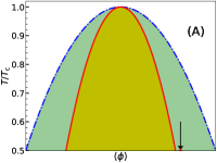
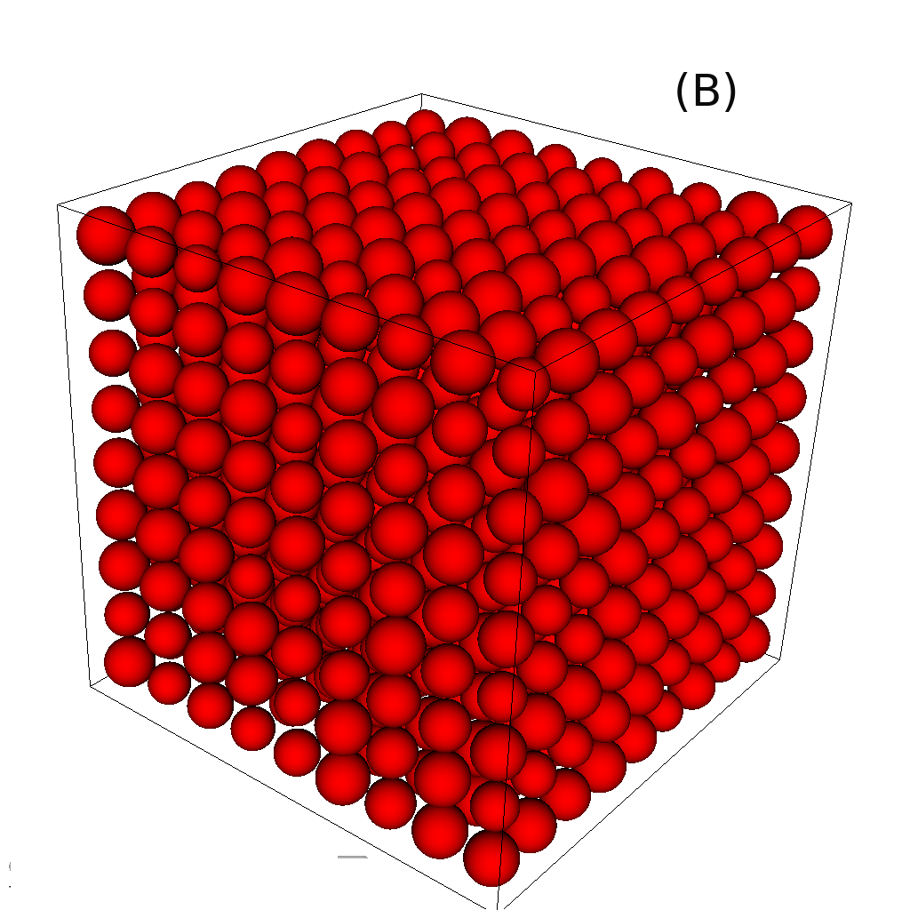
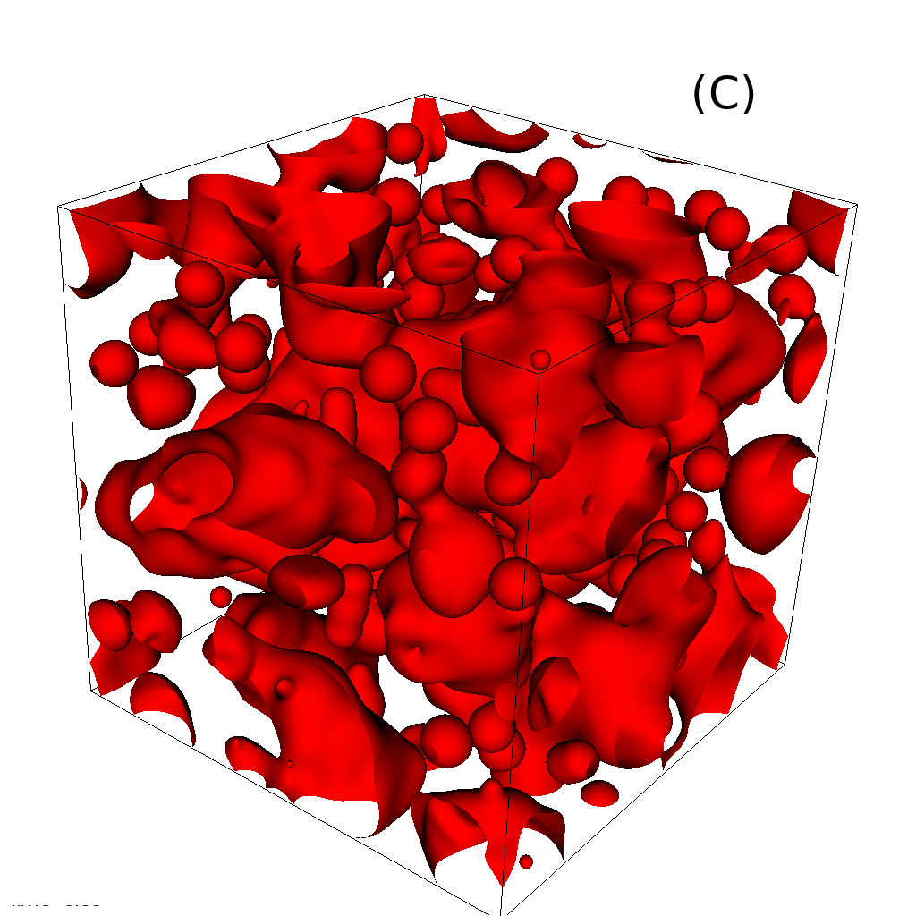
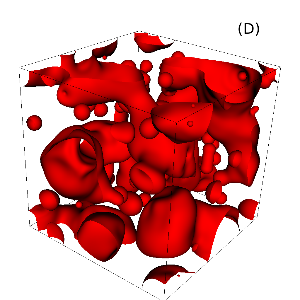
Figure 1: (A) A sketch of the phase-diagram of Landau-Ginzburg type $\phi^{4}$ theory. The blue dashed line is the phase coexistence curve. The red line is the spinodal curve. Near the phase coexistence line droplets form by nucleation. Inside the red line domains grow by spinodal decomposition. The point marked by a red star, pointed at by the arrow, shows our position in this phase-diagram; this is outside the spinodal curve but not too close to the phase coexistence line – droplet spinodal decomposition operates here. (B), (C), (D): Isosurfaces of $\phi$ at $\phi=0$ for $\mbox{La}=10^{5}$ at times $\tau=0$, $18$, and $35$ respectively.

The Cahn–Hilliard–Navier–Stokes equations are given by:

$$\partial_{t}\phi+{\bm{\nabla}}\cdot\bm{J} =0\quad\/.$$ (1a)

$$\bm{J} ={\bm{v}}\phi-\Gamma{\bm{\nabla}}\mu\quad\/.$$ (1b)

$$\mu =\frac{\delta\mathcal{F}}{\delta\phi}\quad\/.$$ (1c)

$$\mathcal{F}[\phi] =\frac{\Lambda}{\xi^{2}}\int d^{d}x\left[f(\phi)+\frac{\xi^{2}}{2}\mid{\bm{\nabla}}\phi\mid^{2}\right]\quad\/.$$ (1d)

$$f(\phi) =\frac{1}{4}\left(1-\phi^{2}\right)^{2}\quad\/.$$ (1e)

$$\rho(\partial_{t}+{\bm{v}}\cdot{\bm{\nabla}}){\bm{v}} =\eta\nabla^{2}{\bm{v}}-\rho{\bm{\nabla}}p-\phi{\bm{\nabla}}\mu\/.$$ (1f)

$${\bm{\nabla}}\cdot{\bm{v}} =0\/.$$ (1g)

Here $\phi$ is the order-parameter, ${\bm{v}}$ the velocity of the flow, $\mu$ the chemical potential, $\Gamma$ the transport coefficient of the chemical potential, $\eta=\rho\nu$ is the dynamic viscosity, $\rho$ is the density, $\nu$ the kinematic viscosity, and $\xi$ is the length-scale the characterizes the interface thickness. The surface tension $\sigma=(2\sqrt{2}/3)\Lambda/\xi$

We use the initial size of the droplets $R$ as the characteristic length scale and $V=\nu/R$ as the characteristic velocity. The non-dimensional parameters are the Laplace number $\mbox{La}\equiv\sigma R/(\rho\nu^{2})$, the Schmidt number $\mbox{Sc}\equiv\nu/D$, and the Cahn number $\mbox{Ch}\equiv\xi/R$, where the diffusivity $D\equiv\Gamma\Lambda/\xi^{2}$. In all our simulations $\mbox{Sc}=1$ and we use several Laplace numbers and two different Cahn numbers. We use a spectral code with periodic boundary conditions with ${\tt N}^{3}$ resolutions where ${\tt N}=512$ and $1024$ – the highest resolution simulations done for this system .

We choose all the droplets to have the same radius $R/\mathcal{L}=1/(8\pi)$ and their centers placed on a cubic lattice. We then add small random perturbations to the radii of the droplets, see Fig. (1B). The initial volume fraction occupied by the droplets (minority phase) is approximately $0.2$ such that $\left\langle\phi\right\rangle=0.62$, where $\left\langle\cdot\right\rangle$ denotes spatial averaging. This choice of $\left\langle\phi\right\rangle$, marked in the phase-diagram, Fig. (1A), puts us in the droplet spinodal decomposition regime Shimizu and Tanaka (2015) – we are neither well inside the spinodal curve nor very close to the co-existence curve.

We show how coarsening progresses in Fig. (1B) to Fig. (1D). At very early times the drops remains practically unchanged in size but move – typically towards their closest neighbour. At $t=0$ there was no flow – the flows that move the droplets are generated by compositional Marangoni effect Shimizu and Tanaka (2015). To confirm, we simulate a collection of seven drops - one central drop at the origin and six drops placed on a cubic lattice around it. Due to the asymmetry all the peripheral drops move towards the central drop and eventually merge into one. A similar experiment where we place the drops on a line also show that drops move toward their nearest neighbours.

We define the structure factor and the energy spectrum as the shell-integrated Fourier spectra of $\phi$ and ${\bm{v}}$ respectively, i.e.,

$$\mathbb{S}(q) \equiv\int\hat{\phi}(\bm{q})\hat{\phi}(-\bm{q})d\Omega\quad\/,$$ (2a)

$$\mathbb{E}(q) \equiv\int\hat{{\bm{v}}}(\bm{q})\hat{{\bm{v}}}(-\bm{q})d\Omega\quad\/,$$ (2b)

where $\hat{\phi}(\bm{q})$ and $\hat{{\bm{v}}}(\bm{q})$ are respectively the Fourier transforms of $\phi({\bm{x}})$ and ${\bm{v}}({\bm{x}})$, $q=\mid\bm{q}\mid$ is the magnitude of the wavevector $\bm{q}$, and $\Omega$ is the solid angle in Fourier space. We calculate the evolving, characteristic length scale, $L$ as Perlekar et al. (2014); Shimizu and Tanaka (2015)

$$K\equiv\frac{\int dqq\mathbb{S}(q)}{\int dq\mathbb{S}(q)}\/\quad{\rm and}\quad L\equiv 2\pi/K$$ (3)

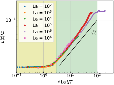
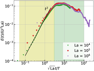
Figure 2: The evolution of the (A) The characteristic length-scale, $L(t)$, and (B) the total kinetic energy $E(t)$ for all the ${\tt A}$ runs, $\mbox{Sc}=1$. The data for different Laplace number collapse on each other when plotted as a function of the scaled time $\tau\equiv\sqrt{\mbox{La}}t/T$.

The time evolution of the characteristic length scale $L(t)$ and the total kinetic energy $E(t)$ are shown in Fig. (2). The evolution for different Laplace numbers collapse when plotted as a function of scaled dimensionless time $\tau\equiv\sqrt{\mbox{La}}(t/T)$. At short times $\tau\lesssim 3$, $L$ is practically a constant – very few droplets have merged. During the same time interval the kinetic energy of the flow grows as $E(t)\sim t^{2}$. At intermediate times $10\lesssim\tau\lesssim 100$ the kinetic energy of the flow remains almost a constant (decreases slowly) while the characteristic length scale grows as $L(t)\sim t^{1/2}$ for at least a decade. We also detect a dependece on Cahn number – the transition to $L\sim t^{1/2}$ happens earlier for larger Cahn number. At very late times $100\lesssim\tau$, as expected, the kinetic energy starts to decay fast while $L$ saturates. The scaling of $L$ with a dynamic exponent of $1/2$ has been observed before in two-dimensional simulations Wu et al. (1995) in the presence of noise and for an off-critical quench but never before in three dimensions .

In Fig. (3) we show representative plots of the compensated structure factor, $q^{2}\mathbb{S}(q)$ and the compensated energy spectrum, $q^{5/3}\mathbb{E}(q)$ for times during which the $L\sim t^{1/2}$ scaling is observed. In both cases we find a region in $q$ over which the compensated plots are approximately horizontal. This implies that over this range of $q$,

$$\mathbb{S}(q)\sim q^{-2}\quad\text{and}\quad\mathbb{E}(q)\sim q^{-5/3}$$ (4)

The change in $\phi$ across a length scale $r$, $\delta_{r}\phi$ has two contributions, one smooth – if $r$ lies either well inside a droplet or well outside droplets – and the another independent of $r$ – if $r$ lies across the boundary of a droplet. In other words, there are isolated jumps connected by smooth regions which implies (Frisch, 1996, section 8.5.2), similar to Burgers equation Aurell et al. (1992), $\mathbb{S}(q)\sim q^{-2}$. The scaling $\mathbb{E}(q)\sim q^{-5/3}$ signifies fully developed turbulence a-la Kolmogorov. This plays a key role in the scaling theory we discuss next.

We construct a scaling theory by generalizing the standard approach Chaikin and Lubensky (1998). From Eq. (1a) the rate of change of characteristic length scale of a droplet is given by $\phi dL/dt\sim J$ where $J\equiv\mid\bm{J}\mid$. Let $\Delta\mu$ be the difference in chemical potential between the two phases. By creating a droplet of size $L$ we both gain, ($\phi\Delta\mu(4/3)\pi L^{3}$) and loose ($-4\pi\sigma L^{2}$) free energy. Minimizing the change in free-energy we estimate $\Delta\mu\approx 2\sigma/(L\phi)$. Typical gradients of chemical potential can then be estimated as ${\bm{\nabla}}\mu\sim\Delta\mu/L\sim 2\sigma/(\phi L^{2})$ We assume that at all times the diffusive contribution to the flux, $J$, in Eq. (1b) is negligible compared to the advective contribution. In addition, at short times the flow velocities are so small that Eq. (1) reduces to,

$$\frac{dL}{dt}\approx 0\quad{\rm and}\quad\partial_{t}{\bm{v}}\approx\phi{\bm{\nabla}}\mu\sim 2\frac{\sigma}{L^{2}}\/.$$ (5)

Then at short times $L(t)$ remains almost a constant and $E(t)\sim t^{2}$ – this rationalizes the short-time behaviour in Fig. (2B).

At intermediate times and at large scales the contribution from the nonlinear term dominates over the viscous term in the momentum equation, Eq. (1f), such that

$$\frac{dL}{dt}\approx\phi v\quad{\rm and}\quad\rho{\bm{v}}\cdot{\bm{\nabla}}{\bm{v}}\sim\phi{\bm{\nabla}}\mu$$ (6)

Next we assume that $\ell$ is the characteristic length scale of the flow. If $\ell$ is proportional to the scale of droplet, $L$, $v\sim\sqrt{\sigma/(\rho L)}$; consequently $\sqrt{L}dL/dt\sim\sqrt{\sigma/\rho}$, which in turn implies $L\sim t^{2/3}$ – Furukawa’s scaling Furukawa (1985). Crucially, if $\ell$ is different from $L$ and is almost a constant at intermediate times we obtain $LdL/dt\sim\sqrt{2\sigma\ell/\rho}$, which implies $L\sim\sqrt{t}$.

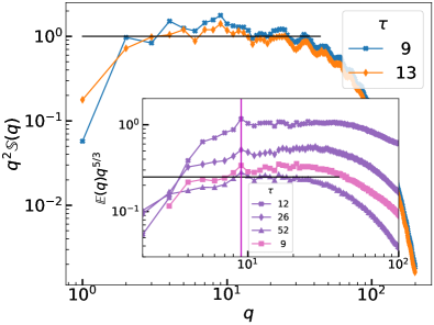
Figure 3: The compensated structure factor, $q^{2}\mathbb{S}(q)$ as a function of $q$ in log-log scale at two different times for the run A6 (${\tt N}=1024$). A range of $q$ over which the compensated plot is flat implies $\mathbb{S}(q)\sim q^{-2}$ over that range. We plot a horizontal line for comparison. Inset: The compensated kinetic energy spectra, $q^{5/3}\mathbb{E}(q)$ as a function of $q$ in log-log scale at three different times for the run A3(${\tt N}=512$) and at $\tau=9$ for the run A6 (${\tt N}=1024$) A range of $q$ over which the compensated spectra is flat implies $\mathbb{E}(q)\sim q^{-5/3}$ over that range. We plot a horizontal line for comparison. The compensated spectra has a peak at $q=q_{\ast}\approx 9$ shown by a vertical line. Note that $q_{\ast}$ does not change with time.

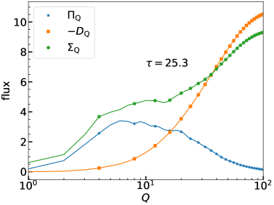
Figure 4: The three terms on the right hand side of the energy flux equation  (8) at an intermediate time $\tau=25.3$.

Let us now critically examine our theory. First, we assume the advective flux dominates over the diffusive flux in Eq. (1b). We find that this is true in our simulations at all times .

Second, at intermediate times ($10\lesssim\tau\lesssim 100$) and at large length scales the nonlinear term in Eq. (1f): (a) dominates over the viscous term; (b) has a characteristic length scale, $\ell$, different from the scale $L$; and (c) the length scale $\ell$ is almost a constant over the timescale. If (a) holds then at large scales the flow must be turbulent and obeys Kolmogorov theory Frisch (1996), i.e., there must exist a range of wavevectors $q$ over which $\mathbb{E}(q)\sim q^{-5/3}$. This is indeed what we have already shown in Fig. (3). Furthermore we notice that the spectra at large scale has a characteristic peak near $q=q_{\ast}\approx 9$ (marked by a vertical line in the inset of Fig. (3)). The location of this peak, $q_{\ast}$ does not change with time. Hence we can define the characteristic length scale of the flow to be $\ell=2\pi/q_{\ast}$ – this scale remains almost a constant during the intermediate times. This confirms both (b) and (c) above.

To directly examine the relative importance of the terms in the momentum equation Eq. (1f) it is usual Frisch (1996) to examine the scale-by-scale energy budget in the Fourier space, defined by

$$\mathcal{E}_{\rm Q}={1\over 2}\int_{0}^{Q}dq\int\mathbb{E}(q)\quad\/.$$ (7)

Straightforward algebra starting from Eq. (1f) shows

$$\partial_{t}\mathcal{E}_{\rm Q}=\Pi_{\rm Q}+D_{\rm Q}-\Sigma_{\rm Q}$$ (8)

where $\Pi_{\rm Q}$, $D_{\rm Q}$ and $\Sigma_{\rm Q}$ are contributions from the nonlinear term, the viscous term, and the $\phi{\bm{\nabla}}\mu$ in Eq. (1f), respectively . The viscous term $D_{\rm Q}$ is always negative whereas both $\Pi_{\rm Q}$ and $\Sigma_{\rm Q}$ can, in principle, have either signs. A positive $\Pi_{\rm Q}$ implies that the kinetic energy cascades from large to small length scales which is the case of Kolmogorov turbulence in three dimensions. The contribution from surface tension $\Sigma_{\rm Q}$, is positive when coagulation of droplets releases free energy that drives the fluid and negative when the flow drives droplet motion. At short times, $\tau\lesssim 3$, as expected, we find that both $\Pi_{\rm Q}$ and $D_{\rm Q}$ are small compared to $\Sigma_{\rm Q}$ , hence  (8) reduces to $\partial_{t}\mathcal{E}_{\rm Q}\approx\Sigma_{\rm Q}$ – supporting the dominant ballance assumed in  (5). This implies $E(t)=\lim_{Q\to\infty}\mathcal{E}_{Q}\sim t^{2}$ – the same scaling we find in Fig. (2B). At intermediate times, for large lengh scale (small enough $Q$, $Q<10$) the contribution from $\phi{\bm{\nabla}}\mu$ is largely ballanced by the nonlinear term, see Fig. (4). Consequently, the dominant ballance in  (8) is $\Sigma_{\rm Q}\approx\Pi_{\rm Q}$ justifying  (6).

Note that turbulence in Cahn–Hilliard–Navier–Stokes equation has been studied extensively but also exclusively with an external stirring force generating and maintaining the turbulence Perlekar et al. (2014); Onuki (2002); Ruiz and Nelson (1981); Fan et al. (2016); Ray and Basu (2011); Pal et al. (2016). By contrast, in our case the turbulence is generated by coagulating droplets. The spectra for both velocity and the phase-variable, $\phi$, shows power-law scaling, i.e., they are scale invariant. Hence each possess only two characteristic length scales, respectively, the large scale and small scale cutoffs of the scaling which are often called the integral scale and the dissipative scale  . We use $\mbox{Sc}=1$, consequently the small scale cutoffs are practically the same. But the large scale cutoffs are very different.

Two related problem are pseudo-turbulence – turbulence generated by rising bubbles Lance and Bataille (1991); Mudde (2005); Prakash et al. (2016); Risso (2018) in a quiescent fluid – and stirred Kolmogorov turbulence modified by rising bubbles Lance and Bataille (1991); Mathai et al. (2020); Pandey et al. (2020, 2021). In both of these cases, coagulation plays negligible role and the effect of the bubbles give rise to the kinetic energy spectrum $\mathbb{E}(q)\sim q^{-3}$  that can be understood by balancing the energy production by the bubbles with the viscous dissipation Lance and Bataille (1991); Prakash et al. (2016); Pandey et al. (2020, 2021). Our simulations corresponds to a very different parameter range where the contribution due to the chemical potential balances the advective nonlinearity.

It has been emphasized before Wagner and Yeomans (1998) that coarsening of the domains in phase-separating binary fluids is not scale-invariant – different characteristic length scales constructed from $\phi$ scales differently. Note that we focus on a very different asepct – we consider only the integral scale, defined in  (3), and show that it scales as $L\sim t^{1/2}$ at intermediate times during which the characteristic length scale of the flow remains almost the same.

In conclusion, we explore the coarsening phenomena at small diffusivity and viscosity in that part of the phase diagram where droplet spinodal decomposition operates. We find turbulence a-la Kolmogorov and emergence of very different characteristic scales of the droplets and the flow – general scale invariance is broken – the integral scale of the droplets $L\sim t^{1/2}$ where the characteristic scale of the flow remains practically constant. Nevertheless, we are able to generalize the standard scaling theory to the present case and obtain clear agreement between theory and simulations. The key to understand the problem is to calculate the scale-by-scale energy budget.

Appendix A Supplemental Material

A.1 Model and Method

Here we provide a detailed description of our model, the numerical method and dimensionless parameters for the direct numerical simulation.

A.1.1 Dynamical equations

We use a phase-field model for binary fluids with a Landau-Ginzburg type $\phi^{4}$ free energy. The dynamics is that of a conserved order parameter coupled to an compressible flow – model H of Hohenberg and Halperin Hohenberg and Halperin (1977) from which the Langvein noise is excluded.

$$(\partial_{t}+{\bm{v}}\cdot{\bm{\nabla}})\phi =\Gamma\nabla^{2}\mu$$ (9a)

$$\mu =\frac{\delta\mathcal{F}}{\delta\phi}$$ (9b)

$$\mathcal{F}[\phi] =\frac{\Lambda}{\xi^{2}}\int d^{d}x\left[f(\phi)+\frac{\xi^{2}}{2}\mid{\bm{\nabla}}\phi\mid^{2}\right]$$ (9c)

$$f(\phi) =\frac{1}{4}\left(1-\phi^{2}\right)^{2}$$ (9d)

$$(\partial_{t}+{\bm{v}}\cdot{\bm{\nabla}}){\bm{v}} =\nu\nabla^{2}{\bm{v}}-{\bm{\nabla}}p-\phi{\bm{\nabla}}\mu$$ (9e)

$${\bm{\nabla}}\cdot{\bm{v}} =0$$ (9f)

As the density of the fluid is constant, we have set it to unity.

A.1.2 Dimensionless parameters

We choose the radius of the droplets, $R$, as our characteristic length scale. There is no characteristic velocity scale set by the initial condition, hence, similar to what is done in convection Landau and Lifshitz (1987), we use $\nu/R$, where $\nu$ is the viscosity, as our characteristic velocity scale to obtain:

$$(\partial_{t}+{\bm{v}}\cdot{\bm{\nabla}})\phi =\frac{1}{\mbox{Sc}}\nabla^{2}\mu\/,$$ (10a)

$$(\partial_{t}+{\bm{v}}\cdot{\bm{\nabla}}){\bm{v}} =\nabla^{2}{\bm{v}}-{\bm{\nabla}}p-\frac{\Phi_{\rm 0}^{1/3}\mbox{La}}{\mbox{Ch}}\phi{\bm{\nabla}}\mu$$ (10b)

Here the four dimensionless numbers are: the Cahn number, $\mbox{Ch}\equiv\xi/\mathcal{L}$, the Schmidt number, $\mbox{Sc}\equiv\nu/D$; the Laplace number, $\mbox{La}\equiv(\sigma R)/\nu^{2}$, where $D\equiv\Gamma\Lambda/\xi^{2}$, $\sigma=(2\sqrt{2}/3)\Lambda/\xi$ and the initial volume fraction occupied by the heavier phase is $\Phi_{\rm 0}$. A different non-dimensionalization Naso and Náraigh (2018) gives Reynolds number $\mbox{Re}=(3/2\sqrt{2})^{1/2}(\mathcal{L}/R)\sqrt{\mbox{La}/\mbox{Ch}}$ and Peclet number $\mbox{Pe}=\mbox{Re}\mbox{Sc}$.

A.1.3 Numerical algorithm, initial condition, and parameters

Our simulations are done in a cubic box of side $2\pi$. This box is discretized in $N$ equally spaced grid points in each direction. Eq. (1) is solved by using a pseudo-spectral method with one-half dealiasing and periodic boundary conditions. We use a second-order Adams-Bashforth scheme for time stepping. An earlier version of this code has been used before in Ref. Perlekar et al. (2014). The velocity is zero at $t=0$. Initial conditions for order parameter $\phi$ are chosen to have an array of droplets as shown in Fig. (1) (B), $\phi=1$ inside the drops and $-1$ outside. Simulation parameters are listed in table 1.

Table 1: Parameters of simulations. The simulations are in $2\pi$ periodic domains in three-dimensions with ${\tt N}^{3}$, ${\tt N}=512$ and $1024$ collocation points. All the simulations have $\mbox{Sc}=1$. Initially, we choose all the droplets to have the same radius $R/\mathcal{L}=1/(8\pi)$ and their centers placed on a cubic lattice. We then add small random perturbations to the radii of the droplets. The initial volume fraction occupied by the droplets (minority phase) is approximately $0.2$ such that $\left\langle\phi\right\rangle=0.62$.

Runs	${\tt N}$	Ch	La
A0	512	$0.19$	$10^{2}$
A1	512	$0.19$	$10^{3}$
A2	512	$0.19$	$10^{4}$
A3	512	$0.19$	$10^{5}$
A4	512	$0.19$	$10^{6}$
A5	512	$0.05$	$10^{6}$
A6	1024	$0.1$	$10^{6}$

A.1.4 Comparison of our parameters with earlier work

Recently Naso and Naráigh Naso and Náraigh (2018) have, for the first time, ventured in to the part of the parameters space with small diffusivisty and viscosity and found signatures of novel coarsening behavior in this regime. Their simulations started with symmetric initial condition whereas we start with droplets organized on a lattice with defects in the droplet-spinodal regime.

Nevertheless it is useful to compare the dimensionless parameters of our simulations with theirs. Ref. Naso and Náraigh (2018) worked with dimensionless viscosity ($1/\mbox{Re}$) and diffusivity ($1/\mbox{Pe}$) and separated the parameters in different phases depending on the types of structures that were observed, not based on the dynamic scaling exponent. Our runs belong to the region on phase space Ref. Naso and Náraigh (2018) called “anomalous” and “inertial”

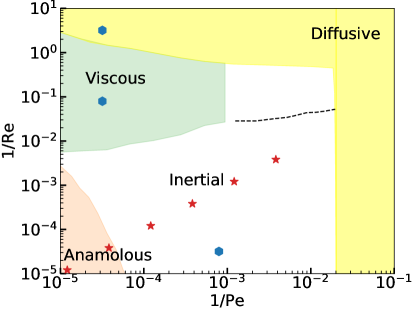
Figure 5: The phase diagram in the $1/\mbox{Pe}$–$1/\mbox{Re}$ plane according to Ref. Naso and Náraigh (2018). The points marked by red star are our simulations. We have also used our code to simulate the system with symmetric initial condition for the points marked in blue and have obtained results that agree with Ref. Naso and Náraigh (2018).

In the notation of Ref. Naso and Náraigh (2018) the Cahn–Hilliard–Navier–Stokes equations are:

$$\rho D_{t}{{\bm{u}}} =\eta\nabla^{2}{{\bm{u}}}-\nabla P-\phi\nabla\mu,$$ (11)

$$D_{t}\phi =\frac{D}{\alpha}\nabla^{2}\mu,$$ (12)

$$\mu =\alpha(-\phi+\phi^{3}-\xi^{2}\nabla^{2}\phi)~{}\rm{with}~{}\alpha\equiv\frac{\Lambda}{\xi^{2}}.$$ (13)

Choosing the velocity scale as $U\equiv\sqrt{\alpha/\rho}$, the length scale $\mathcal{L}$ (box size) we obtain the following dimensionless equations

$$\rho D_{t}{{\bm{u}}} =\frac{1}{\mbox{Re}}\nabla^{2}{{\bm{u}}}-\nabla P-\phi\nabla\mu,$$ (14)

$$D_{t}\phi =\frac{1}{\mbox{Pe}}\nabla^{2}\mu,$$ (15)

$$\mu =(-\phi+\phi^{3}-\mbox{Ch}^{2}\nabla^{2}\phi),$$ (16)

with $\Re\equiv U\mathcal{L}/\nu$, $\mbox{Ch}=\xi/\mathcal{L}$ and $\mbox{Pe}=U\mathcal{L}/D$; the Reynolds number, the Cahn number and Peclet number respectively, see Table 2.

Table 2: Dimensionless numbers for our runs. Based on the values of $1/Pe$ and $1/Re$, we are in the anamolous regime of Ref. Naso and Náraigh (2018).

Run	$D$	$\Lambda$	$\xi$	$\nu$	Ch	Pe	Re
A0	$5\cdot 10^{-4}$	$2.6\cdot 10^{-2}$	$2.45\cdot 10^{-2}$	$5\cdot 10^{-4}$	$3.9\cdot 10^{-3}$	$8.27\cdot 10^{3}$	$8.27\cdot 10^{3}$
A1	$5\cdot 10^{-4}$	$2.6\cdot 10^{-3}$	$2.45\cdot 10^{-2}$	$5\cdot 10^{-4}$	$3.9\cdot 10^{-3}$	$2.62\cdot 10^{3}$	$2.62\cdot 10^{3}$
A2	$5\cdot 10^{-4}$	$2.6\cdot 10^{-4}$	$2.45\cdot 10^{-2}$	$5\cdot 10^{-4}$	$3.9\cdot 10^{-3}$	$8.27\cdot 10^{4}$	$8.27\cdot 10^{4}$
A3	$5\cdot 10^{-4}$	$2.6\cdot 10^{-5}$	$2.45\cdot 10^{-2}$	$5\cdot 10^{-4}$	$3.9\cdot 10^{-3}$	$2.61\cdot 10^{4}$	$2.61\cdot 10^{4}$

A.2 Fluxes

The standard approach to understand scaling behaviour in turbulence is to calculate the scale-by-scale energy budget equation Frisch (1996). Here we follow the procedure outline in Perlekar et al. (2014). Multiplying  (9a) by $\hat{\phi}(-\bm{q})$ and integrating over all the fourier modes upto wave-number $Q$, we obtain

$$\partial_{t}\mathcal{S}_{\rm Q}+\mathcal{A}_{\rm Q}=\mathcal{G}_{\rm Q}$$ (17)

where $\mathcal{A}_{\rm Q}$ is the contribution from the advective term and $\mathcal{G}_{\rm Q}$ is the contribution from the diffusive term. In particular,

$$\mathcal{A}_{\rm Q} \equiv\Re\left\{\int_{0}^{Q}\int_{\Omega}\hat{\phi}(-\bm{q})\widehat{[{\bm{v}}\cdot{\bm{\nabla}}\phi]}(\bm{q})dqd\Omega\right\}\/,$$ (18a)

$$\mathcal{G}_{\rm Q} \equiv\Re\left\{\Gamma\int_{0}^{Q}\int_{\Omega}\hat{\phi}(-\bm{q})\widehat{[\nabla^{2}\mu]}(\bm{q})dqd\Omega\right\}\/.$$ (18b)

In Fig. (6) we show two representative plots of these two fluxes as a function of the wavenumber $Q$, one at short times and the other at intermediate times. We find that in all cases and at all $Q$, except for very high $Q$, the advective flux dominates over the diffusive contribution.

By multiplying the Fourier transformed Eq. (9e) with $\hat{{\bm{v}}}{(-\bm{q})}$, and integrating over all the fourier modes upto wave-number $Q$, we obtain

$$\partial_{t}\mathcal{E}_{\rm Q}=\Pi_{\rm Q}+D_{\rm Q}-\Sigma_{\rm Q}.$$ (19)

Here $\mathcal{E}_{\rm Q}$ is the cumulative kinetic energy. The rest of the quantities in  (19) are defined as follows:

$$\Pi_{\rm Q} \equiv-\Re\left\{\int_{0}^{Q}\int_{\Omega}\hat{{\bm{v}}}(-\bm{q})\cdot\widehat{[{\bm{v}}\cdot{\bm{\nabla}}{\bm{v}}]}(\bm{q})dqd\Omega\right\}$$ (20a)

$$D_{\rm Q} \equiv-\nu\int_{0}^{Q}q^{2}\mathbb{E}(q)dq$$ (20b)

$$\Sigma_{\rm Q} \equiv\Re\left\{\int_{0}^{Q}\int_{\Omega}\hat{{\bm{v}}}(-\bm{q})\cdot\widehat{[\phi\nabla\mu]}(\bm{q})dqd\Omega\right\}$$ (20c)

In Fig. (7) we show a representative plot of all the three contributions on the right hand side of  (19) at short times. Clearly $\Sigma_{\rm Q}$ dominates over the other two. Hence we conclude that the system is not in a stationary state – the growth of kinetic energy is fuelled by the contribution from $\phi{\bm{\nabla}}\mu$.

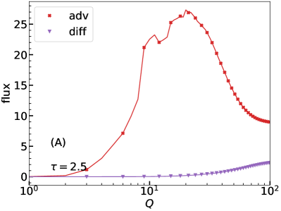
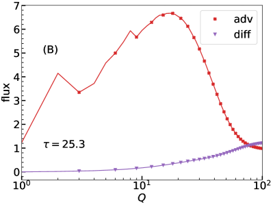
Figure 6: Contribution to the flux of $\phi$ from the advective(${\bm{v}}\cdot{\bm{\nabla}}\phi$) and the diffusive ($\Gamma\nabla^{2}\mu$) term at early times (A) and intermediate times (B).

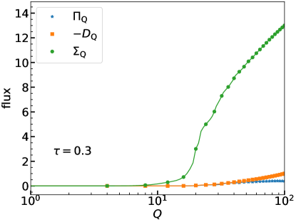
Figure 7: Contribution to the flux of energy from the nonlinear term ($\Pi_{\rm Q}$), the viscous term ($D_{\rm Q}$) and surface tension ($\Sigma_{\rm Q}$) at early time.