BFAR – Bounded False Alarm Rate detector for improved radar odometry estimation

Abstract

This paper presents a new detector for filtering noise from true detections in radar data, which improves the state of the art in radar odometry. Scanning Frequency-Modulated Continuous Wave (FMCW) radars can be useful for localisation and mapping in low visibility, but return a lot of noise compared to (more commonly used) lidar, which makes the detection task more challenging. Our Bounded False-Alarm Rate (BFAR) detector is different from the classical Constant False-Alarm Rate (CFAR) detector in that it applies an affine transformation on the estimated noise level after which the parameters that minimize the estimation error can be learned. BFAR is an optimized combination between CFAR and fixed-level thresholding. Only a single parameter needs to be learned from a training dataset. We apply BFAR to the use case of radar odometry, and adapt a state-of-the-art odometry pipeline (CFEAR), replacing its original conservative filtering with BFAR. In this way we reduce the state-of-the-art translation/rotation odometry errors from 1.76%/0.5^∘/100 m to 1.55%/0.46^∘/100 m; an improvement of 12.5%.

I Introduction

There is a great need for enabling mobile robots and self-driving cars to robustly operate in all seasons, weather and visibility conditions. While these are challenging conditions for vision and lidar, Frequency-Modulated Continuous Wave radars are not affected by smoke, dust, rain or fog, and can detect obstacles regardless of visibility settings. Recently, radars, and especially spinning FMCW radars have become compact, accurate and gained popularity and demonstrated more resilient localisation and mapping [1]. This makes them suitable for applications in harsh environments; e.g., underground mines [2] and fire fighting [3] tasks. Unfortunately, radar suffer from high level of noise and clutter from multipath reflections. Previous filters have required tuning of several parameters, been sensitive to changes in environment [4, 5], required an extensive amount of training data [4, 6] or provided too few detections [7, 8]. For that reason, we present a novel target detection BFAR that improve on existing noise filtering techniques in order to detect only useful radar features. We demonstrate our filter on the previously existing pipeline for radar odometry   Conservative Filtering for Efficient and Accurate Radar odometry (CFEAR), depicted in Fig. 1), which improves state-on-the-art from 1.76% to 1.54% translation error on the Oxford Radar RobotCar dataset (an improvement of 12.5%).

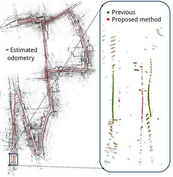
Figure 1: The Proposed radar detector BFAR yields high detection quality and can be used to improve radar odometry pipelines such as “CFEAR”. [7]

The paper is structured as follows. Sec. II gives a more in-depth description of the common problems with radar detection, and gives an intuition for our solution. Sec. III covers related work. Then in Sec. IV we present BFAR in detail, a parameter estimation procedure and the adopted odometry pipeline CFEAR. Finally, results and conclusions are discussed in Sections V and Sec. VI.

II Problem formulation

Target detection from radar signals faces several challenges: the unstable and highly variable noise floor, speckle noise, ghost targets (false positive detection due to multi-path reflections), receiver saturation, and finally that highly reflective targets usually appear in several range-cells instead of only one, which reduces accuracy. We propose a new detector for radar signals and show how it improves radar-only odometry estimation. Even though we apply this detector specifically for FMCW radar in this paper, it can be extended to many other applications that have similar noise issues.

There is an agreement among researchers on radar odometry that the classical CFAR detection methods are not directly suitable for this application. For example, the Cell-Averaging CFAR (CA-CFAR) detector, a common variant of CFAR that computes a threshold for each cell that is proportional to the average of surrounding cells in a sliding window analysis, is not very useful with the odometry estimation pipeline in [7]. It requires specifying precisely the values of Probability of False-Alarm ($P_{\mathit{FA}}$), within a limited range, in order to have the algorithm working properly. Larger values of $P_{\mathit{FA}}$ will return many detections from noise which makes odometry estimation much more challenging, while smaller values will return very few detections which also will cause odometry estimation to fail. Fig. 2 presents the odometry estimation error against $P_{\mathit{FA}}$ values for CA-CFAR.

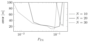
Figure 2: The sensitivity of odometry estimation absolute trajectory error vs $P_{\mathit{FA}}$ values of the CA-CFAR detector. The plots corresponding to an example from the Oxford RobotCar dataset [9]. The parameter $N$ is half the sliding window length when computing the cell averaging.

It shows that the error rapidly increases outside a certain $P_{\mathit{FA}}$ range. Unfortunately, this range is not known, and it is hard to predict. Therefore, using point clouds filtered with CFAR for radar odometry tends to fail, unless one has a good and data-specific idea about selecting a suitable value (as also demonstrated in Sec.V-B). Our proposed BFAR method makes the selection of $P_{\mathit{FA}}$ much more flexible.

The design of a detector is usually started from specifying the $P_{\mathit{FA}}$. The optimum detector is the one that maximizes the Probability of Detection ($P_{D}$) for a given $P_{\mathit{FA}}$. (See Fig. 3 for graphical illustration). In a stationary noise environment, a fixed-threshold detector can achieve the optimum detector performance if the noise power is known. In practice, the noise power is not known, therefore a statistical estimator is used to estimate its value. Additionally, the noise is usually mixed with clutter (reflections from objects other than the target: buildings, trees, ground surface, etc.) and therefore is non-stationary. For both reasons, the fixed threshold is replaced by an adaptive detector, usually a CFAR variant, to have a controlled False-Alarm Rate (FAR).

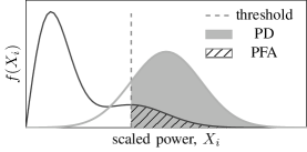
Figure 3: Graphical representation of the $P_{\mathit{FA}}$ and $P_{D}$, the shaded areas, for a single sample $X_{i}$. The black density is the PDF of $X_{i}$ when there is only noise, while the gray density is the PDF of $X_{i}$ when there is a target.

In the literature, there are many detection algorithms for radar signals that are based on the CFAR detector strategy. The basic idea of CFAR is to set a different threshold $T$ for each Cell Under Test (CUT), using a constant multiplied by the estimated noise level at that cell. The constant is computed from a specified FAR and the estimated noise level $Z$ is found using some statistical analysis on the $N$ neighboring cells.

$$T=\text{constant}\times Z$$ (1)

This scheme has the advantage of changing the threshold for each cell according to the estimated noise level but also has a clear drawback; since $Z$ is a random variable with variance, a large constant multiplier results in an amplified threshold variance by, the square of the constant. This scheme fails to achieve the specified constant FAR when we have a bad estimator of the noise level from neighboring cells and the actual FAR could be larger or smaller.

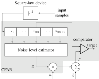
Figure 4: The structure of BFAR detector. It is at a glance similar to CFAR but fundamentally different as it applies linear transformation on the estimated noise level. Notice that, in this manuscript, we always use four guard-samples two on each side of $X_{\text{CUT}}$ which are not shown in this figure to perceive the simplicity.

In this paper, we present a new detection algorithm that is based on a different strategy than CFAR. It can handle the variable noise floor in a better way than the standard CFAR and does so by selecting a threshold from an affine transformation of the estimated noise level $Z$, as explained in Fig. 4. The transformation requires two parameters: scale $a$ and offset $b$. The scale is selected to ensure that the threshold variance does not increase dramatically, while the offset parameter is selected to control $P_{\mathit{FA}}$. In this setup, both $P_{D}$ and $P_{\mathit{FA}}$ will depend on the unknown noise power, which might seem to be undesirable. However, their values will be controlled in such a way that $P_{\mathit{FA}}$ and $P_{D}$ will decrease as the noise power is decreased, and they increase with increased noise but will not exceed a specified upper bound. Most importantly, this control is done automatically as will be shown in Sec. IV when deriving the $P_{\mathit{FA}}$ equation. In other words, instead of maintaining $P_{\mathit{FA}}$ constant but with large variance as in CFAR, BFAR fixes the Probability of False-Alarm upper-bound ($P_{\mathit{FAub}}$) and sets $P_{\mathit{FA}}$ with lower variance compared to CFAR.

The threshold in BFAR for each cell is then

$$T=a\times Z+b.$$ (2)

The affine transformation will not give a constant FAR but will give FAR that is bounded from above – hence the name BFAR. Learning the best values for the parameters can be done using grid search on a training dataset, (as demonstrated in Sec. IV-B). We assume here the values of $a$ and $b$ are fixed and not changing during the estimation process.

Notice that in Fig. 4 the noise level estimator block is generic, therefore it is possible to apply the BFAR structure on most CFAR variants by plugging-in the corresponding noise estimation block without further modifications.

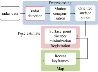
Figure 5: Overview of CFEAR radar odometry, used for evaluating BFAR radar detection. In the previously published version of CFEAR [7], the radar detection block uses a $k$-strongest detector. We replace this block with BFAR and show how it leads to a new state of the art in radar odometry.

To evaluate and examine the performance of BFAR, we include it in the recent radar odometry pipeline CFEAR [7], depicted in Fig. 5. CFEAR is an efficient and accurate pipeline for incremental pose estimation that operates on $360^{\circ}$ spinning radar data, producing state-of-the-art accuracy in terms of low odometry drift.

CFEAR extracts features in a two-step approach that first applies a conservative filter in polar space, keeping the $k$ strongest returns for each azimuth angle, and then computes a sparse set of oriented surface points in Cartesian space. The sparse set of surface points is registered jointly to a history of key frames in order to estimate the pose and velocity of the radar. The estimated velocity is used to perform motion compensation.

In the original publication [7], CFEAR radar odometry was optimized to be fast and efficient, using a conservative $k$-strongest filter (with $k=12$ detections per azimuth) that typically removes secondary landmarks, even though these could be used for increased accuracy. For that reason, the conservative filter can be replaced with our proposed filter, which produces improved detections compared to the conservative filter, and can additionally aid odometry estimation.

We use odometry quality as an indirect measure of detection performance, assuming that a good detector produces consistent and stable landmarks and are suitable for odometry. However, our method should be applicable for other perception tasks.

In Sec. V we show quantitative results on the Oxford Radar RobotCar dataset and demonstrate that CFEAR radar odometry with BFAR detection instead of $k$-strongest produces new state-of-the-art accuracy for radar-only odometry.

III Related work

III-A radar only odometry estimation

Previous methods for radar odometry overcome radar noise by learning to extract key points [5, 6], remove noise [10, 4, 5, 10] – or by applying learning-free approaches that analyze intensity of reflections [11, 12, 7, 1, 13, 1].

Filter free approaches for odometry were investigated by Hong [1] et al., who extracted and matched SURF features; and Park [14] et al., who proposed a method for dense matching of raw radar images. However, these methods have demonstrated relatively high odometry errors compared to the current state of the art. A similar dense matching technique was proposed by Barnes et al., which additionally uses self-supervision from ground truth poses for learning to mask out noise. Unfortunately, the odometry quality is reduced when operating in environments that was not in the training set, despite using a large amount of training data. Kung et al. applied a fixed intensity threshold to discard weak potentially spurious reflections [13]. A more refined, though still ad-hoc, method, was successfully used by Adolfsson et al. [7], which additionally bounds the number of returned reflections to improve efficiency. Cen et al. [11, 12] investigated approaches for extracting features by analyzing image intensity and gradients.

Until today, the top performing method for radar odometry is CFEAR, despite that the original publication integrates a conservative filter designed to omit non-primary, but potentially important landmarks [7]. In the present work, we replace their conservative filter with our proposed BFAR method for higher quality detections, and accordingly, improve odometry estimation.

III-B fixed-level detector

Some authors have used simple fixed-level thresholding instead of an adaptive method like CFAR [1, 13, 3], however, selecting a suitable threshold value is not trivial. For example, Hong [1] extracted only peaks that are greater than a standard deviation of mean intensity per azimuth. Kung et al. [13] suggest keeping all points exceeding a noise threshold, which needs to be learned offline. Adolfsson et al. [7] showed that this can have a negative impact on efficiency and may have negative impact on map quality. Other researchers suggested conservative filtering [8, 7]. The most restricted one, used by Marck et al. [8], keeps only the strongest reflection per azimuth, which will neglect a lot of potentially important information and possible good landmarks. Adolfsson et al. in CFEAR [7] relaxed this a little bit to keep $k$ strongest returns per azimuth, using values of $k=6\sim 12$. They presented very good results in terms of translation and rotation errors on the Oxford public robotcar dataset [9]. For this reason, and also to make the results directly comparable, we will use the same odometry estimation pipeline presented in [7] but replacing the $k$-strongest filter with our proposed detector.

III-C CFAR detector

The principle of CFAR was first described in 1968 by Finn and Johnson [15], they presented what is now known as CA-CFAR. Since then, CFAR has been extensively studied in the literature and many variants, more than 25 [16], have been proposed. We will give a brief review on CFAR since it is the main part of the proposed detector. The main challenges facing CFAR [17] detectors are the following.

• Mutual-target-masking, preventing the detection due to threshold increasing when a target falls within the reference cells. Smallest Of Cell Averaging CFAR (SOCA-CFAR), Trimmed Mean CFAR (TM-CFAR) [18], Censored CFAR (CS-CFAR) and Ordered Statistics CFAR (OS-CFAR) [19] solve the mutual-target-masking problem [20].

• Clutter boundaries, the abrupt change in the interference power – solved using Greatest Of Cell Averaging CFAR (GOCA-CFAR).

• Multiple-targets in the neighboring cells.

• Non-homogeneous noise or clutter. [18, 21, 22, 23].

The last two are still an active research directions and many researchers contribute continuously. One reason behind that could be the new development in sensors technology and the new challenging noise therein.

The performance of the CA-CFAR detector was presented in [20] for one or more interfering targets presented in the noise-level estimating cells. They also presented censored CFAR to maintain acceptable performance in the presence of interfering targets. An analysis of the performance of CA-CFAR, GOCA-CFAR, SOCA-CFAR, OS-CFAR, and TM-CFAR in homogeneous and nonhomogeneous backgrounds was presented in [18]. They computed the average detection threshold for each scheme to compare detection performance. To obtain closed-form expressions, they used an exponential noise model for clear and clutter backgrounds.

Automatic censored CFAR detection for nonhomogeneous environments was first presented in [21], and a variability index to distinguish between homogeneous and nonhomogeneous noise in [22]. The OS-CFAR analyzed in [19] for CFAR loss, $P_{\mathit{FA}}$, and $P_{D}$. The performance analysis of Censored Mean Level Detector CFAR (CMLD-CFAR) presented in [24] and the TM-CFAR detector, a generalization of OS-CFAR and CMLD-CFAR detector presented in [18].

Recently, the OS-CFAR and its derivatives are the most commonly used for detection. The developments mainly focus on how to distinguish between cells from homogeneous noise and others from nonhomogeneous noise to decide which cell to keep and which to remove from the estimation process. Automatic censoring based on ordered data difference was proposed in [25]. A robust control scheme for adjusting detection threshold of CFAR presented in [23]. The cell-averaging clutter-map (CA-CM) with variability indexes suggested by [26].

The structure of BFAR presented in Fig. 4 makes it possible to use most of the CFAR variants above, however, we will consider only CA-CFAR for simplicity and a proof of concept.

IV Bounded False-Alarm Rate (BFAR)

IV-A Mathematical derivation

In this section we will give the derivation of $P_{\mathit{FA}}$ for our proposed BFAR detector. We will assume the cell-averaging noise estimation in Fig. 4 for simplicity and comparison purposes with CA-CFAR.

We will use the following assumptions:

• Assuming independent and Gaussian noise, then the output of square-low detector will be exponentially distributed and independent, with PDF

  $$f(X_{i})=\frac{1}{2\lambda}\text{exp}\left(\frac{-X_{i}}{2\lambda}\right),\qquad x\geq 0$$ (3)

  and

  $$\lambda=\begin{cases}\mu&,\qquad\text{under H}_{0}\\ \mu(S+1)&,\qquad\text{under H}_{1}\end{cases}$$ (4)

  where

  • H₀ is the null hypothesis of no target, so $X_{i}$ contains only noise,

  • H₁ is the alternative hypothesis of presence of a target,

  • $S$ is the average signal-to-noise ratio (SNR) of a target,

  • $\mu$ is the total background clutter-plus-thermal noise power, its value is not fixed and is changing from cell-to-cell according to unknown but continuous and smooth function (no fast changes are expected).

• The detector performance is determined by the average detection and false alarm probabilities. We will follow the same procedure as in [18], the $P_{\mathit{FA}}$ is, (see also Fig. 3)

  $$\text{\acs{PFA}}=\mathbb{E}\left[p\left(X_{\text{CUT}}>aZ+b\left|\text{H}_{0}\right.\right)\;\left|\;Z\right.\right]$$ (5)

  $$= \mathbb{E}\left[\int_{aZ+b}^{\infty}\frac{1}{2\mu}\text{exp}\left(\frac{-y}{2\mu}\right)dy\right]$$ (6)

  $$= \mathbb{E}\left[\text{exp}\left(-\frac{aZ+b}{2\mu}\right)\right]$$ (7)

  $$= \mathbb{E}\left[\text{exp}\left(-\frac{aZ}{2\mu}\right)\right]\mathbb{E}\left[\text{exp}\left(\frac{-b}{2\mu}\right)\right]$$ (8)

  $$= M_{Z}\left(\frac{a}{2\mu}\right)\text{exp}\left(\frac{-b}{2\mu}\right)$$ (9)

  where $M_{Z}(\cdot)$ denotes the moment generating function (mgf) of the random variable $Z$.

• For a cell-averaging processor operating on $2N$ samples, the random variable $Z$ will be

  $$Z\mathrel{\mathop{:}}=\sum_{i=1}^{2N}X_{i}$$ (10)

  where $X_{i}$ are the samples of the neighboring cells. From [18], the distribution of $Z$ will be

  $$Z\sim\Gamma\left(2N,2\mu\right),$$ (11)

  and the corresponding mgf is

  $$M_{y}(u)=\left(1+2\mu u\right)^{-2N}.$$

  Substituting this in Equ. (9) above, we obtain

  $$\text{\acs{PFA}}=\left(1+a\right)^{-2N}\text{exp}\left(\frac{-b}{2\mu}\right).$$ (12)

Setting the parameter $b=0$, Equ. (12) will be reduced to

$$\text{\acs{PFA}}=\left(1+a\right)^{-2N}\qquad\text{for}\leavevmode\nobreak\ b=0$$ (13)

which is exactly the $P_{\mathit{FA}}$ equation for CA-CFAR, (the expression and derivation in [18]). Setting $a=0$ will give

$$\text{\acs{PFA}}=\text{exp}\left(\frac{-b}{2\mu}\right)\qquad\text{for}\leavevmode\nobreak\ a=0$$ (14)

which is the $P_{\mathit{FA}}$ for a fixed-level detector. So BFAR with cell-averaging can be seen as a generalization for the classical CA-CFAR detector. The smaller values of $\mu$ compared to $b$ correspond to a smaller exponential term in (12) which makes the value of $P_{\mathit{FA}}$ even smaller. On the other hand, very large values of $\mu$ compared to $b$ make the exponential term closer to one and the $P_{\mathit{FA}}$ simplifies to

$$\text{\acs{PFA}}\approxeq\text{\acs{PFA}}_{ub}\mathrel{\mathop{:}}=\left(1+a\right)^{-2N}$$ (15)

which is the upper-bound for its value. Then we rewrite (12) as

$$\text{\acs{PFA}}=\text{\acs{PFA}}_{ub}\leavevmode\nobreak\ \text{exp}\left(\frac{-b}{2\mu}\right).$$ (16)

When the parameter $a=0$, both $P_{\mathit{FA}}$ and $P_{D}$ will be directly related to the background noise level $\mu$.

In a similar way we derive an expression for $P_{D}$:

$$= \mathbb{E}\left[p\left(X_{\text{CUT}}>aZ+b\left|\text{H}_{1}\right.\right)\;\left|\;Z\right.\right]$$ (17)

$$= \left(1+\frac{a}{1+S}\right)^{-2N}\text{exp}\left(\frac{-b}{2\mu\left(1+S\right)}\right).$$ (18)

The exponential term in (18) will indeed reduces $P_{D}$ compared to CA-CFAR.

IV-B Parameter learning

It is clear from (12) that we need to tune $N$ and the two parameters $a$ and $b$ for the detector, which is not straightforward especially because the value of $\mu$ is not known. Therefore we propose the following procedure:

• First, with a specified value of $N$ and $P_{\mathit{FAub}}$, the parameter $a$ can be computed from the $P_{\mathit{FAub}}$ using (15),

• Second, the parameter $b$ can be learned from a use-case relevant data set. For the present paper, we are mainly interested in radar odometry, and use a training data set with ground-truth pose information (from GNSS) and learn $b$ using a suitable grid search method

• Finally, use the obtained parameter values in our detection algorithm for radar data.

V Experimental validation

V-A Methodology

We investigated the performance of the proposed detection algorithm on odometry estimation using the Oxford Radar RobotCar dataset [27, 9]. It has both radar raw data and ground-truth information for the odometry. The evaluation is performed using the standard odometry benchmark from KITTI [28] to compute the following performance metrics:

• Average sub-sequence translational and rotational errors, by evaluating possible sub-sequences of length (100, 200, $\ldots$,800) meters.

• Absolute Trajectory Error (ATE): the Root-Mean-Square Error (RMSE) between estimated poses and corresponding ground truth.

To learn the offset parameter $b$, we select one sequence from the dataset. With $N=20$ and parameter grid $a=[0,0.1,0.25,0.5,1,2,3]$, $b=[5,10,15,20,30,40,50,60]$, we record the odometry metrics to find the best value for the parameters. As stated above, since $N$ is fixed the values of $P_{\mathit{FAub}}$ can be computed directly from $a$ to be $[1,0.0115,0.0003,9.5\times 10^{-07},2.9\times 10^{-10},9.1\times 10^{-13}]$. The smallest translation error, rotation error and ATE achieved during this grid search corresponds to $a=1$ or $\text{\acs{PFAB}}=9.5\times 10^{-07}$ and $b=20$ in the training dataset. See grid plot in Fig. 6.

Sequence Method resolution 10-12-32 16-13-09 17-13-26 18-14-14 18-15-20 10-11-46 16-11-53 18-14-46 mean mean SCV CFEAR-BFAR (ours) 0.043 1.48/0.42 1.54/0.43 1.52/0.44 1.49/0.45 1.45/0.44 1.54/0.45 1.65/0.49 1.65/0.50 1.55/0.46 1.55/0.46 CFEAR-k12 [7] 0.043 1.64/0.48 1.86/0.52 1.66/0.48 1.71/0.49 1.75/0.51 1.65/0.48 1.99/0.53 1.79/0.5 1.76/0.50 1.76/0.50 Cen2018 [11] 0.175 N/A N/A N/A N/A N/A N/A N/A N/A $3.72/0.95$ $3.63/0.96$ Hong odometry [1] 0.043 2.98/0.8 3.12/0.9 2.92/0.8 3.18/0.9 2.85/0.9 3.26/0.9 3.28/0.9 3.33/1 3.11/0.9 3.11/0.9 Under the radar [6] 0.346 N/A N/A N/A N/A N/A N/A N/A N/A 2.0583/0.67 N/A Hero [5] 0.2628 *1.77/0.62 *1.75/0.59 *2.04/0.73 *1.83/0.61 *2.20/0.77 *2.14/0.71 *2.01/0.61 *1.97/0.65 *1.96/0.66 N/A Barnes Dual Cart [4] 0.043 N/A N/A N/A N/A N/A N/A N/A N/A 1.16/0.3 2.7848/0.0085 Kung [13] $0.125$ N/A N/A N/A N/A N/A N/A N/A N/A 1.9584/0.6 1.9584/0.6 SuMa (Lidar) [29] N/A 1.1/0.3 1.2/0.4 1.1/0.3 0.9/0.1 1.0/0.2 1.1/0.3 0.9/0.3 1.0/0.1 1.16/0.3 1.16/0.3

Table I: Evaluation on 8 sequences with different methods and sensor modalities on the Oxford radar RobotCar dataset [27]. Results are given in (% translation error / deg/100 m). “*” indicates that the results are not exactly comparable due to lacking spatial cross validation.

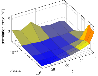
Figure 6: Translation error surface with $P_{\mathit{FAub}}$ and $b$ for $N=20$.

V-B Odometry estimation performance compared to CA-CFAR

Fig. 7 shows the plots of the different evaluation metrics vs $P_{\mathit{FAub}}$ with parameter $b$. Notice that in the case of $b=0$ (blue curves) , the detector will be CA-CFAR and $P_{\mathit{FAub}}$ is exactly equal to $P_{\mathit{FA}}$ values. Comparing BFAR with CFAR, we can see that BFAR works well even with $\acs{PFAB}=1$. Comparing this with the limited selection of $P_{\mathit{FA}}$ in CFAR, as presented in Fig. 2, proves the flexibility in parameter selection and also the ability to automatically account for changes in background noise level. Notice that for $\acs{PFAB}=1$, it will be a fixed-level detector and the value of $b=40$ will give the smallest value for ATE.

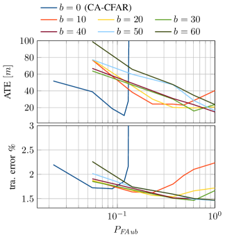
Figure 7: BFAR estimation evaluation metrics vs the $P_{\mathit{FAub}}$. When $b=0$, BFAR is the same as CA-CFAR.

V-C Odometry estimation performance

We apply the learned and optimized parameters, $a=1$ and $b=20$, and insert BFAR in the CFEAR odometry pipeline for evaluation on the remaining sequences of the robotcar dataset. Except for the detector, we used the same parameters of CFEAR as in the original publication [7].

The obtained odometry errors are presented in Tab. I and compared to seven recent radar odometry baselines, as well as one baseline using lidar odometry for reference. Compared to the state of the art, CFEAR with BFAR detection consistently has smaller error over all the trajectories.

VI Conclusion

This paper focuses on radar detection for radar-only odometry estimation. We have proposed a new detector called BFAR and showed that, compared to CA-CFAR, its parameters can be easily trained such that it keeps relevant detections and removes radar noise. In particular, we have demonstrated the usefulness of BFAR by incorporating it in the CFEAR pipeline for radar odometry, which to date holds the lowest published odometry errors in the Oxford Radar RobotCar dataset. Using the classical CA-CFAR detector with CFEAR will not lead to acceptable performance and the pipeline may fail. However, it was possible to achieve even smaller estimation errors than the original CFEAR when using our new BFAR detector instead of the baseline $k$-strongest detector. Conceptually, BFAR can be seen as an optimized combination between CA-CFAR and fixed-level thresholding to minimize the odometry estimation error. It was possible to reduce the estimation translation/rotation errors in CFEAR from 1.76%/0.5${}^{\circ}/100$m to 1.55%/0.46${}^{\circ}/100$m.

The structure of BFAR makes it possible to use many variants of CFAR to add their advantages, not necessarily the classical CA-CFAR that we used here for simplicity and proof of concept. Finally, even though the BFAR detector has been proposed specifically for spinning radar odometry estimation, it is expected to contribute in signal detection for other tasks and sensors with similar noise issues.

References

- [1] Z. Hong, Y. Petillot, and S. Wang, “Radarslam: Radar based large-scale slam in all weathers,” in 2020 (IROS), 2020, pp. 5164–5170.
- [2] G. Brooker, R. Hennessey, C. Lobsey, M. Bishop, and E. Widzyk-Capehart, “Seeing through dust and water vapor: Millimeter wave radar sensors for mining applications,” Journal of Field Robotics, vol. 24, no. 7, pp. 527–557, 2007.
- [3] M. Mielle, M. Magnusson, and A. J. Lilienthal, “A comparative analysis of radar and lidar sensing for localization and mapping,” in Proceedings of the European Conference on Mobile Robots (ECMR), Sept. 2019.
- [4] D. Barnes, R. Weston, and I. Posner, “Masking by moving: Learning distraction-free radar odometry from pose information,” in CoRL, ser. CoRL, L. P. Kaelbling, D. Kragic, and K. Sugiura, Eds., vol. 100. PMLR, 30 Oct–01 Nov 2020, pp. 303–316.
- [5] K. Burnett, D. J. Yoon, A. P. Schoellig, and T. D. Barfoot, “Radar odometry combining probabilistic estimation and unsupervised feature learning,” 2021.
- [6] D. Barnes and I. Posner, “Under the radar: Learning to predict robust keypoints for odometry estimation and metric localisation in radar,” in (ICRA), 2020, pp. 9484–9490.
- [7] D. Adolfsson, M. Magnusson, A. Alhashimi, A. J. Lilienthal, and H. Andreasson, “CFEAR radarodometry–conservative filtering for efficient and accurate radar odometry,” arXiv preprint arXiv:2105.01457, 2021.
- [8] J. W. Marck, A. Mohamoud, E. vd Houwen, and R. van Heijster, “Indoor radar SLAM: A radar application for vision and GPS denied environments,” in 2013 European Radar Conference. IEEE, 2013, pp. 471–474.
- [9] W. Maddern, G. Pascoe, C. Linegar, and P. Newman, “1 Year, 1000km: The Oxford RobotCar Dataset,” The International Journal of Robotics Research (IJRR), vol. 36, no. 1, pp. 3–15, 2017.
- [10] R. Aldera, D. De Martini, M. Gadd, and P. Newman, “Fast radar motion estimation with a learnt focus of attention using weak supervision,” in 2019 International Conference on Robotics and Automation (ICRA). IEEE, 2019, pp. 1190–1196.
- [11] S. H. Cen and P. Newman, “Precise ego-motion estimation with millimeter-wave radar under diverse and challenging conditions,” in 2018 IEEE International Conference on Robotics and Automation (ICRA). IEEE, 2018, pp. 1–8.
- [12] ——, “Radar-only ego-motion estimation in difficult settings via graph matching,” in 2019 International Conference on Robotics and Automation (ICRA). IEEE, 2019, pp. 298–304.
- [13] P.-C. Kung, C.-C. Wang, and W.-C. Lin, “A normal distribution transform-based radar odometry designed for scanning and automotive radars,” arXiv preprint arXiv:2103.07908, 2021.
- [14] Y. S. Park, Y.-S. Shin, and A. Kim, “Pharao: Direct radar odometry using phase correlation,” in 2020 IEEE International Conference on Robotics and Automation (ICRA). IEEE, 2020, pp. 2617–2623.
- [15] H. Finn, “Adaptive detection mode with threshold control as a function of spatially sampled clutter-level estimates,” RCA Rev., vol. 29, pp. 414–465, 1968.
- [16] J. R. Machado-Fernández, N. Mojena-Hernández, and J. d. l. C. Bacallao-Vidal, “Evaluation of cfar detectors performance,” Iteckne, vol. 14, no. 2, pp. 170–178, 2017.
- [17] D. Vivet, P. Checchin, and R. Chapuis, “Localization and mapping using only a rotating FMCW radar sensor,” Sensors, vol. 13, no. 4, pp. 4527–4552, 2013.
- [18] P. P. Gandhi and S. A. Kassam, “Analysis of CFAR processors in nonhomogeneous background,” IEEE Transactions on Aerospace and Electronic systems, vol. 24, no. 4, pp. 427–445, 1988.
- [19] N. Levanon, “Detection loss due to interfering targets in ordered statistics CFAR,” IEEE transactions on aerospace and electronic systems, vol. 24, no. 6, pp. 678–681, 1988.
- [20] J. T. Rickard and G. M. Dillard, “Adaptive detection algorithms for multiple-target situations,” IEEE Transactions on Aerospace and Electronic Systems, no. 4, pp. 338–343, 1977.
- [21] S. D. Himonas and M. Barkat, “Automatic censored CFAR detection for nonhomogeneous environments,” IEEE Transactions on Aerospace and Electronic systems, vol. 28, no. 1, pp. 286–304, 1992.
- [22] A. Farrouki and M. Barkat, “Automatic censoring CFAR detector based on ordered data variability for nonhomogeneous environments,” IEEE Proceedings-Radar, Sonar and Navigation, vol. 152, no. 1, pp. 43–51, 2005.
- [23] J. H. Shin and Y. Choi, “Robust control for the detection threshold of CFAR process in cluttered environments,” Sensors, vol. 20, no. 14, p. 3904, 2020.
- [24] J. A. Ritcey, “Performance analysis of the censored mean-level detector,” IEEE Transactions on Aerospace and Electronic Systems, no. 4, pp. 443–454, 1986.
- [25] W. Jiang, Y. Huang, and J. Yang, “Automatic censoring CFAR detector based on ordered data difference for low-flying helicopter safety,” Sensors, vol. 16, no. 7, p. 1055, 2016.
- [26] X. Yang, K. Huo, J. Su, X. Zhang, and W. Jiang, “An anti-FOD method based on CA-CM-CFAR for MMW radar in complex clutter background,” Sensors, vol. 20, no. 6, p. 1635, 2020.
- [27] D. Barnes, M. Gadd, P. Murcutt, P. Newman, and I. Posner, “The Oxford radar robotcar dataset: A radar extension to the Oxford robotcar dataset,” arXiv preprint arXiv: 1909.01300, 2019.
- [28] A. Geiger, P. Lenz, and R. Urtasun, “Are we ready for autonomous driving? The KITTI vision benchmark suite,” in Vision and Pattern Recognition (CVPR), 2012.
- [29] J. Behley and C. Stachniss, “Efficient surfel-based SLAM using 3D laser range data in urban environments,” in Systems (RSS), 2018.