Hybrid Transceiver Design for Tera-Hertz MIMO Systems Relying on Bayesian Learning Aided Sparse Channel Estimation

Abstract

Hybrid transceiver design in multiple-input multiple-output (MIMO) Tera-Hertz (THz) systems relying on sparse channel state information (CSI) estimation techniques is conceived. To begin with, a practical MIMO channel model is developed for the THz band that incorporates its molecular absorption and reflection losses, as well as its non-line-of-sight (NLoS) rays associated with its diffused components. Subsequently, a novel CSI estimation model is derived by exploiting the angular-sparsity of the THz MIMO channel. Then an orthogonal matching pursuit (OMP)-based framework is conceived, followed by designing a sophisticated Bayesian learning (BL)-based approach for efficient estimation of the sparse THz MIMO channel. The Bayesian Cramer-Rao Lower Bound (BCRLB) is also determined for benchmarking the performance of the CSI estimation techniques developed. Finally, an optimal hybrid transmit precoder and receiver combiner pair is designed, which directly relies on the beamspace domain CSI estimates and only requires limited feedback. Finally, simulation results are provided for quantifying the improved mean square error (MSE), spectral-efficiency (SE) and bit-error rate (BER) performance for transmission on practical THz MIMO channel obtained from the HIgh resolution TRANsmission (HITRAN)-database.

I Introduction

Tera-Hertz (THz) wireless systems are capable of supporting data rates up to several Tera-bits per second (Tbps) [han2018propagation, chen2019survey, faisal2020ultramassive] in the emerging 6G landscape. The availability of large blocks of spectrum in the THz band, in the range of $0.1$ THz to $10$ THz, can readily fulfil the ever-increasing demand for data rates. This can in turn support several bandwidth-thirsty applications such as augmented reality (AR), virtual reality (VR), wireless backhaul and ultra-high speed indoor communication [han2018propagation]. However, due to their high carrier frequency, THz signals experience severe propagation losses and blockage, beyond a few meters. Moreover, the high molecular absorption due to the vibrations of the molecules at specific frequencies, and the higher-order reflections [jornet2011channel] become cumbersome in the THz band. Hence, the practical realization of THz systems faces numerous challenges. A promising technique of overcoming these obstacles is constituted by multiple-input multiple-output (MIMO) solutions relying on antenna arrays, which are capable of improving the signal strength at the receiver via the formation of ‘pencil-sharp beams’ having ultra-high directional gains [sarieddeen2020overview]. However, the conventional MIMO transceiver architecture, wherein each transmit and receive antenna is connected to an individual radio frequency (RF) chain, becomes unsuitable at such high frequencies, mainly due to the power hungry nature of the analog-to-digital converters coupled with their high sampling-rate [he2020beamspace]. Hence, the hybrid transceiver architecture, originally proposed by Molish et al. in their pioneering work [molisch2017hybrid, zhang2005variable], is an attractive choice for such systems, since it allows the realization of a practical transceiver employing only a few RF chains. Furthermore, in conventional MIMO systems, the various signal processing operations are typically implemented in the digital domain. By contrast, the signal processing tasks are judiciously partitioned between the RF front-end and baseband processor in a hybrid MIMO transceiver, with the former handling the analog processing via analog phase shifters (APSs), while the latter achieves baseband processing in a digital signal processor (DSP). Naturally, the overall performance of the hybrid architecture, for example, its achievable spectral-efficiency (ASE) and bit-error-rate (BER), critically depend on the design of the baseband and RF precoder/ combiner, which ultimately relies on the accuracy of the available channel state information (CSI). Thus, high-precision channel estimation holds the key for attaining robust performance and ultimately for realizing the full potential of THz MIMO systems. A detailed overview and a comparative survey of the related works is presented next.

I-A Related Works and Contributions

The pioneering contribution of Jornet and Akyildiz [jornet2011channel] developed a novel channel model for the entire THz band, i.e. for the band spanning $0.1-10$ THz. Their ground-breaking work relied on the concepts of radiative transfer theory [goody1995atmospheric] and molecular absorption for developing a comprehensive model [rothman2009hitran]. Their treatise evaluated the total path-loss by meticulously accounting for the molecular absorption, the reflections as well as for the free-space loss components. Later Yin and Li [lin2015adaptive] developed a general MIMO channel model for a hybrid THz system and subsequently proposed distance-aware adaptive beamforming techniques for improving the signal-to-noise power ratio (SNR). However, their framework assumes the availability of perfect CSI, which is rarely possible in practice. To elaborate, CSI estimation in a THz hybrid MIMO system is extremely challenging owing to the low SNR and massive number of antenna elements. Hence, the conventional Least Square (LS) and Minimum Mean Square Error (MMSE)-based CSI estimation would incur an excessive pilot-overhead. Therefore, they are unsuitable for CSI acquisition in practical THz systems.

Early solutions [9454383, alkhateeb2014channel, 9445013, el2014spatially, srivastava2019quasi, gao2019wideband, 9165794, 8732197] proposed for the milli-meter wave (mmWave) band exploited the angular-sparsity of the channel to achieve improved CSI estimation and tracking at a substantially reduced pilot-overhead. Several optimization and machine learning based algorithms are also proposed for hybrid transceiver design in mmWave MIMO systems. In this context, the authors of [8329410] proposed joint beam selection and precoder design for maximizing the sum-rate of a downlink multiuser mmWave MIMO system under transmit power constraints. The pertinent optimization problem has been formulated as a weighted minimum mean squared error (WMMSE) problem, which is then efficiently solved using the penalty dual decomposition method. A joint hybrid precoder design procedure has been described in [8606437] for full-duplex relay-aided multiuser mmWave MIMO systems, considering also the effects of imperfect CSI. The authors of [9110863] and [9610037] successfully developed two-timescale hybrid precoding schemes for maximizing the sum-rate, and reducing the complexity and CSI feedback overhead. A frame-based transmission scenario is considered in their work, wherein each frame comprises a fixed number of time slots. The long-timescale RF precoders are designed based on the available channel statistics and are updated once in a frame. By contrast, the short-timescale baseband precoders are optimized for each time slot based on the low-dimensional effective CSI. Hence, an optimization based solution is developed in [9110863], whereas a deep neural network (DNN)-aided technique is designed in [9610037]. The angular-sparsity is also a key feature of the THz MIMO channel [sarieddeen2020overview, yan2019dynamic], which arises due to the highly directional beams of large antenna arrays, coupled with high propagation losses and signal blockage in the THz regime. In fact, Sarieddeen et al. [sarieddeen2020overview] showed that the THz MIMO channel is more sparse than its mmWave counterpart. However, there are only a few recent studies, such as [schram2018compressive, schram2019approximate, ma2020joint], which develop sparse recovery based CSI estimation techniques for THz MIMO systems. A brief review of these and the gaps in the existing THz literature are described next.

The early work of Gao et al. [gao2016fast] successfully developed an a priori information aided fast CSI tracking algorithm for discrete lens antenna (DLA) array based THz MIMO systems. Their model relies on a practical user mobility trajectory [zhou1999tracking] to develop a time-evolution based framework for the angle of arrival (AoA)/ angle of departure (AoD) of each user. Subsequent contributions in this direction, such as [stratidakis2019cooperative] and [stratidakis2020low], consider base station (BS) cooperation and a multi-resolution codebook, respectively, for improving the accuracy of channel tracking obtained via the a priori information aided scheme of [gao2016fast]. However, this improved tracking accuracy is achieved at the cost of inter-BS cooperation, which necessitates additional infrastructure and control overheads. Kaur et al. [kaur2020enhanced] developed a model-driven deep learning technique for enhancing the channel tracking accuracy in a THz MIMO system. Their algorithm relies on a deep convolutional neural network trained offline in advance to learn the non-linear relationship between the estimates based on [gao2016fast] and the original channel. Another impressive contribution [he2020beamspace] by He et al. proposes a model-driven unsupervised learning network for beamspace channel estimation in wide-band THz MIMO systems. Furthermore, a deep learning assisted signal detection relying on single-bit quantization is proposed in the recent contribution [9536661]. A fundamental limitation of [gao2016fast, stratidakis2019cooperative, stratidakis2020low, kaur2020enhanced] is that they consider single antenna users. More importantly, their estimation accuracy is highly sensitive to the accuracy of the time-evolution model employed and they do not incorporate the effect of molecular absorption into their THz channel, which renders the model inaccurate in reproducing the true radio propagation environment.

Schram et al. [schram2019approximate] employed an approximate message passing (AMP)-based framework for CSI estimation in THz systems. The sparse channel estimation framework developed considers only a single-input single-output (SISO) THz system, where the channel impulse response (CIR) is assumed to be sparse. Ma et al. [ma2020joint] conceived sparse beamspace CSI estimation for intelligent reflecting surface (IRS)-based THz MIMO systems. The optimal design of the phase shift matrix at the IRS has been determined in their work based on the BS to IRS and IRS to user equipment (UE) THz MIMO channels. Recent treatises, such as [dovelos2021channel, sha2021channel, balevi2021wideband], address the problem of wideband CSI acquisition in THz systems. Specifically, Dovelos et al. [dovelos2021channel] consider an orthogonal frequency division multiplexing (OFDM)-based THz hybrid MIMO system and develop orthogonal matching pursuit (OMP)-based techniques for CSI estimation. Balevi and Andrews [balevi2021wideband] have considered generative adversarial networks for channel estimation in an OFDM-based THz hybrid MIMO system. On the other hand, Sha and Wang [sha2021channel] derived a CSI estimation and equalization technique for a single-carrier THz SISO system accounting also for realistic RF impairments. A list of novel contributions of our paper is presented next. Our novel contributions are also boldly and explicitly contrasted to the existing literature in Table-I.

TABLE I: Boldly contrasting our novel contributions to the state-of-the-art

Feautures	[jornet2011channel]	[he2020beamspace]	[lin2015adaptive]	[ma2020joint]	[kaur2020enhanced]	[gao2016fast]	[schram2019approximate]	[balevi2021wideband]	[dovelos2021channel]	[sha2021channel]	Proposed
THz hybrid MIMO			✓	✓				✓	✓		✓
APSs-based hybrid architecture			✓	✓				✓	✓		✓
Single antenna users		✓	✓		✓	✓	✓		✓		✓
CSI estimation		✓		✓	✓	✓	✓	✓	✓	✓	✓
Diffused-ray modeling											✓
Angular-sparsity		✓	✓	✓		✓	✓		✓		✓
Molecular absorption losses	✓		✓						✓		✓
Reflection losses			✓						✓		✓
Optimal pilot design										✓	✓
Transceiver design				✓					✓		✓
Optimal power allocation			✓								✓
Limited CSI feedback											✓
MSE lower bound									✓	✓	✓

I-B Novel Contributions

1. We commence by developing a practical distance and frequency dependent THz MIMO channel model that also incorporates the molecular absorption and reflection losses together with the traditional free-space loss. Note that almost all the existing contributions utilize the classical Saleh-Valenzuela channel model of [lin2015indoor], which does not consider the diffused rays for each multipath component together with first- and second-order reflections. Furthermore, the path-gains in most of the existing treatises are simply modeled as Rayleigh fading channel coefficients without considering the molecular absorption and multiple reflections. Hence, an important aspect of the channel model developed is that it incorporates several diffused rays for each of the reflected multipath components including their associated reflection and molecular absorption losses. This results in broadening of the beamwidths of the signals and mimics a practical THz MIMO channel.

2. The existing research on the development of sparse CSI estimation schemes for a point-to-point analog phase shifter (APS) based hybrid MIMO THz system is very limited, since most of them have considered only single-antenna users, focusing predominantly on discrete lens antenna (DLA) arrays. Hence for considering a point-to-point APS-based hybrid MIMO architecture, an efficient frame-based channel estimation model is developed, which frugally employs a low number of pilot beams for exciting the various angular modes of the channel. Subsequently, using a suitable ‘sparsifying’-dictionary, a beamspace representation is developed for the THz MIMO channel, followed by the pertinent sparse channel estimation model. For this, BL-based channel estimation techniques are derived for exploiting the sparsity of the THz MIMO channel. Note that the proposed BL-based technique is novel in the context of THz MIMO channel estimation, since it has not been explored as yet in THz hybrid MIMO systems.

3. The design of the optimal pilot beams used for CSI estimation, which can significantly enhance sparse signal recovery, has not been considered in the existing THz literature either. Moreover, it is also desirable to develop bounds to benchmark the performance of the CSI estimation schemes. To this end, another key contribution of this work is the design of a specific pilot matrix that minimizes the so-called ‘total-coherence’ defined in [elad2007optimized, li2013projection] for enhancing the performance of sparse signal recovery. Furthermore, to benchmark the MSE performance of our sparse CSI estimators, the Bayesian Cramer-Rao lower bound (BCRLB) is also derived for the CSI estimates.

4. To the best of our knowledge, the existing hybrid transceiver design approaches found in the THz literature, such as [yuan2018hybrid], assume the availability of perfect CSI, which is impractical due to the large number of antennas, resulting in excessive pilot overheads. Crucially, no joint beamspace channel estimation and hybrid transceiver design procedure is available in the THz literature. To address this problem, a capacity-approaching hybrid transmit precoder (TPC) and MMSE-optimal hybrid receiver combiner (RC) are developed, which can directly employ the estimate of the beamspace domain channel obtained from the proposed CSI estimators. The proposed algorithm requires only limited CSI of the beamspace channel, namely the non-zero coefficients and their respective indices, which substantially reduces the feedback required. Furthermore, in contrast to the existing hybrid transceiver designs [alkhateeb2014channel, el2014spatially, 9179621, 9395091], the proposed hybrid transceiver design requires no iterations, and hence it is computationally efficient.

5. Our simulation results demonstrate the enhanced performance of our channel estimators, TPC and RC for various practical simulation parameters. In this context, this paper calculates the molecular absorption coefficient using the parameters obtained from the HITRAN database [hitran], which is suitable for the entire THz band, specifically for the higher end spanning $1$ to $10$ THz. On the other hand, most of the existing works employ models, which are only valid for the lower end around $0.1$ to $0.3$ THz.

I-C Organization and Notation

The main focus of this work is on hybrid transceiver design relying on the BL-based estimated beamspace domain CSI. To achieve this, in Section-II, we begin with the THz MIMO system and channel model, which incorporates the specific molecular absorption and reflection losses arising in the THz regime. This is followed by developing its sparse beamspace domain representation and a novel frame-based channel estimation model in Section-III, which excites various angular modes of the THz MIMO channel. Furthermore, in order to improve the sparse CSI estimation performance, the mutual coherence of the equivalent sensing matrix has also been minimized in Section-III, which results in the optimal choice of the training precoders/combiners to be employed during channel estimation. Subsequently, the proposed BL and MBL-based sparse channel estimation schemes are developed in Section-IV, which is followed by the BCRLB for benchmarking their CSI estimation performance. Finally, based on the estimated CSI, the problem of designing the capacity-optimal hybrid precoder and MMSE-optimal hybrid combiner is addressed in Section-V. Our simulation results are presented in Section-LABEL:sec:simulation_results, followed by our conclusions in Section-LABEL:sec:conclusion.

Notation: The notation $\mathrm{floor}[a]$ represents the greatest integer, which is less than $a$, whereas $\mathrm{rem}[a,b]$ denotes the remainder, when $a$ is divided by $b$; the $i$th element of the vector $\mathbf{a}$ and $(i,j)$th element of the matrix $\mathbf{A}$ are denoted by $\mathbf{a}(i)$ and $\mathbf{A}(i,j)$, respectively; $\mathbf{I}_{N}$ denotes an identity matrix of size $N$; $\mathrm{vec}(\mathbf{A})$ vectorizes the columns of the matrix $\mathbf{A}$ and $\mathrm{vec}^{-1}(\mathbf{a})$ denotes the inverse vectorization operation; the Kronecker product of two matrices $\mathbf{A}$ and $\mathbf{B}$ is denoted by $\mathbf{A}\otimes\mathbf{B}$; the $l_{2}$- and Frobenius-norm are represented by $\|\cdot\|_{2}$ and $\|\cdot\|_{F}$, respectively.

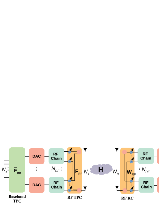
Figure 1: Block diagram of a THz hybrid MIMO system.

II THz MIMO System and Channel Model

The schematic of our THz hybrid MIMO system is portrayed in Fig. 1, where $N_{T}$ and $N_{R}$ denote the number of transmit antennas (TAs) and receive antennas (RAs), respectively, whereas $N_{\text{RF}}$ denotes the number of RF chains. Furthermore, $N_{S}$ is the number of data streams, where $N_{S}\leq N_{\text{RF}}$, while $N_{\text{RF}}<<\min(N_{T},N_{R})$ [ma2020joint, sarieddeen2020overview]. The transmitter is composed of two major blocks, the digital baseband TPC $\bar{\mathbf{F}}_{\text{BB}}\in\mathbb{C}^{N_{\text{RF}}\times N_{S}}$ and the analog RF TPC $\bar{\mathbf{F}}_{\text{RF}}\in\mathbb{C}^{N_{T}\times N_{\text{RF}}}$. At the receiver side, $\bar{\mathbf{W}}_{\text{RF}}\in\mathbb{C}^{N_{R}\times N_{\text{RF}}}$ denotes the RF RC, whereas $\bar{\mathbf{W}}_{\text{BB}}\in\mathbb{C}^{N_{\text{RF}}\times N_{S}}$ represents the baseband RC. As described in [ma2020joint, sarieddeen2020overview], the analog RF TPC $\bar{\mathbf{F}}_{\text{RF}}$ and RC $\bar{\mathbf{W}}_{\text{RF}}$ are comprised of APSs. Hence, for simplicity, these are constrained as $|\bar{\mathbf{F}}_{\text{RF}}(i,j)|=\frac{1}{\sqrt{N_{T}}},|\bar{\mathbf{W}}_{\text{RF}}(i,j)|=\frac{1}{\sqrt{N_{R}}},\forall i,j$. Thus, the baseband system model of our THz MIMO system is given by

$$\bar{\mathbf{y}}=\bar{\mathbf{W}}_{\text{BB}}^{H}\bar{\mathbf{W}}_{\text{RF}}^{H}\mathbf{H}\bar{\mathbf{F}}_{\text{RF}}\bar{\mathbf{F}}_{\text{BB}}\bar{\mathbf{x}}+\bar{\mathbf{W}}_{\text{BB}}^{H}\bar{\mathbf{W}}_{\text{RF}}^{H}\bar{\mathbf{v}},$$ (1)

where $\bar{\mathbf{y}}\in\mathbb{C}^{N_{S}\times 1}$ is the signal vector received at the output of the baseband RC, $\bar{\mathbf{x}}\in\mathbb{C}^{N_{S}\times 1}$ represents the transmit baseband signal vector at the input of the baseband TPC, whereas the quantity $\bar{\mathbf{v}}\in\mathbb{C}^{N_{R}\times 1}$ is the complex additive white Gaussian noise (AWGN) at the receiver having the distribution of $\mathcal{CN}\left(\mathbf{0}_{N_{R}\times 1},\sigma_{v}^{2}\textbf{I}_{N_{R}}\right)$. The matrix $\mathbf{H}\in\mathbb{C}^{N_{R}\times N_{T}}$ in (1) represents the baseband equivalent of the THz MIMO channel, whose relevant model is described next.

II-A THz MIMO Channel Model

As described in [lin2015adaptive], the THz MIMO channel can be modeled as the aggregation of a line-of-sight (LoS) and a few NLoS components. The LoS propagation results in a direct path between the BS and the UE, whereas the NLoS propagation results in some indirect multipath rays after reflection from the various scatterers present in the environment. Thus, the THz MIMO channel $\mathbf{H}$, which is a function of the operating frequency $f$ and distance $d$, can be expressed as

$$\mathbf{H}(f,d)=\mathbf{H_{\text{LoS}}}(f,d)+\mathbf{H_{\text{NLoS}}}(f,d),$$ (2)

where the LoS and NLoS components are given by

$$\mathbf{H_{\text{LoS}}}(f,d) =\sqrt{\frac{N_{T}N_{R}}{N_{\text{ray}}}}\sum_{j=1}^{N_{\text{ray}}}\alpha_{\text{L},j}(f,d)G_{t}^{a}G_{r}^{a}\mathbf{a}_{r}\left(\phi_{\text{L},j}^{r}\right)\mathbf{a}_{t}^{H}\left(\phi_{\text{L},j}^{t}\right),$$ (3)

$$\mathbf{H_{\text{NLoS}}}(f,d) =\sqrt{\frac{N_{T}N_{R}}{N_{\text{NLoS}}N_{\text{ray}}}}\sum\limits_{i=1}^{N_{\text{NLoS}}}\sum_{j=1}^{N_{\text{ray}}}\alpha_{i,j}(f,d)G_{t}^{a}G_{r}^{a}\mathbf{a}_{r}\left(\phi_{i,j}^{r}\right)\mathbf{a}_{t}^{H}\left(\phi_{i,j}^{t}\right).$$ (4)

Here, the quantities $\alpha_{\text{L},j}(f,d)$ and $\alpha_{i,j}(f,d)$ represent the complex-valued path-gains of the LoS and NLoS components, respectively, $N_{\text{NLoS}}$ denotes the number of NLoS multipath components, whereas $N_{\text{ray}}$ signifies the number of diffused-rays in each multipath component. Furthermore, $G_{t}^{a}$ and $G_{r}^{a}$ represent the TA and RA gains, respectively. The quantities $\phi^{r}_{\text{L},j}$ and $\phi^{t}_{\text{L},j}$ denote the AoA and AoD of the $j$th ray in the LoS multipath component, respectively, whereas $\phi^{r}_{i,j}$ and $\phi^{t}_{i,j}$ represent the AoA and AoD of the $j$th diffuse-ray in the $i$th NLoS multipath component. The vectors $\mathbf{a}_{r}(\phi^{r})\in\mathbb{C}^{N_{R}\times 1}$ and $\mathbf{a}_{t}(\phi^{t})\in\mathbb{C}^{N_{T}\times 1}$ denote the array response vectors of the uniform linear array (ULA) corresponding to the AoA $\phi^{r}$ at the receiver and AoD $\phi^{t}$ at the transmitter, respectively. These are defined as

$$\mathbf{a}_{r}(\phi^{r})=\displaystyle\frac{1}{\sqrt{N_{R}}}\Big{[}1,e^{-j\frac{2\pi}{\lambda}d_{r}\cos\left(\phi^{r}\right)},\ldots,e^{-j\frac{2\pi}{\lambda}{(N_{R}-1)}d_{r}\cos\left(\phi^{r}\right)}\Big{]}^{T},$$ (5)

$$\mathbf{a}_{t}(\phi^{t})=\displaystyle\frac{1}{\sqrt{N_{T}}}\Big{[}1,e^{-j\frac{2\pi}{\lambda}d_{t}\cos\left(\phi^{t}\right)},\ldots,e^{-j\frac{2\pi}{\lambda}{(N_{T}-1)}d_{t}\cos\left(\phi^{t}\right)}\Big{]}^{T},$$ (6)

where $d_{r}$ and $d_{t}$ represent the antenna-spacings at the receiver and transmitter, respectively, and $\lambda$ denotes the operating wavelength.

Let the complex path-gain $\alpha(f,d)$ be expressed as $\alpha(f,d)=|\alpha(f,d)|e^{j\psi}$, where $|\alpha(f,d)|$ is the magnitude of the complex path-gain and $\psi$ is the associated independent phase shift. According to [lin2015adaptive, jornet2011channel], the magnitude of the LoS path gain $|\alpha_{\text{L},j}(f,d)|$ can be modeled as

$$|\alpha_{\text{L},j}(f,d)|^{2}=L_{\text{spread}}(f,d)L_{\text{abs}}(f,d),$$ (7)

where $L_{\text{spread}}(f,d)$ and $L_{\text{abs}}(f,d)$ represent the spreading (or the free-space) and molecular absorption losses respectively, which are given by

$$L_{\text{abs}}(f,d)=e^{-k_{\text{abs}}(f)d},\ \ L_{\text{spread}}(f,d)=\left(\frac{c}{4\pi fd}\right)^{2}.$$ (8)

Here, $c$ denotes the speed of light in vacuum and $k_{\text{abs}}(f)$ is the molecular absorption coefficient. Similarly, for the $j$th diffuse-ray of the $i$th NLoS multipath component, the magnitude of the complex path-gain can be expressed as [lin2015adaptive, sarieddeen2020overview]

$$\left|\alpha_{i,j}(f,d)\right|^{2}=\Gamma_{i,j}^{2}(f)L_{\text{spread}}(f,d)L_{\text{abs}}(f,d),$$ (9)

where $\Gamma_{i,j}(f)$ denotes the first-order reflection coefficient of the $j$th diffuse-ray of the $i$th NLoS component. For higher-order reflections, the equivalent reflection coefficient is equal to the product of individual reflection coefficients of the respective scattering media. Further details on the calculation of the absorption coefficient $k_{\text{abs}}(f)$ and the reflection coefficient $\Gamma_{i,j}(f)$ are given in the subsequent subsections.

II-B Calculation of the Reflection Coefficient $\Gamma(f)$

Due to the small wavelength of the THz signal, the reflection coefficient $\Gamma(f)$ is an important parameter to be taken into account while evaluating the losses of the NLoS components [piesiewicz2007scattering, lin2015adaptive]. This is in turn defined in terms of the Fresnel reflection coefficient $(\gamma)$ and the Rayleigh roughness factor $(\varrho)$, as $\Gamma(f)=\gamma(f)\varrho(f),$ where the coefficients $\gamma(f)$ and $\varrho(f)$ are given by:

$$\gamma(f)=\frac{Z(f)\cos\left(\theta_{\text{in}}\right)-Z_{0}\cos\left(\theta_{\text{ref}}\right)}{Z(f)\cos\left(\theta_{\text{in}}\right)+Z_{0}\cos\left(\theta_{\text{ref}}\right)}\text{ \ and \ }\varrho(f)=e^{-\tfrac{1}{2}\left(\tfrac{4\pi f\sigma\cos\left(\theta_{\text{in}}\right)}{c}\right)^{2}}.$$ (10)

In the above expressions, $\theta_{\text{in}}$ denotes the angle of incidence, while $\theta_{\text{ref}}$ represents the angle of refraction, which obeys $\theta_{\text{ref}}=\sin^{-1}\left(\sin(\theta_{\text{in}})\frac{Z(f)}{Z_{0}}\right)$. The quantity $Z(f)$ denotes the wave impedance of the reflecting medium, whereas $Z_{0}=377\,\Omega$ represents the wave impedance of the free space and $\sigma$ in (10) denotes the standard deviation of the reflecting surface’s roughness.

II-C Absorption Coefficient $k_{\text{abs}}(f)$ [jornet2011channel]

As described in [jornet2011channel], the absorption coefficient $k_{\text{abs}}(f)$ of the propagation medium at frequency $f$ can be evaluated as

$$k_{\text{abs}}(f)=\sum_{i,g}k_{\text{abs}}^{i,g}(f),$$ (11)

where, $k_{\text{abs}}^{i,g}$ denotes the absorption coefficient of the $i$th isotopologue of the $g$th gas. The quantity $k_{\text{abs}}^{i,g}(f)$ can be mathematically defined as

$$k_{\text{abs}}^{i,g}(f)=\left(\frac{p}{p_{0}}\right)\left(\frac{T_{\text{STP}}}{T}\right)Q^{i,g}\sigma^{i,g}(f),$$ (12)

where $p$ and $T$ denote the system pressure and temperature, respectively, while $T_{\text{STP}}$ and $p_{0}$ represent the temperature at standard pressure and reference pressure, respectively. The quantity $\sigma^{i,g}$ denotes the absorption cross-section of the $i$th isotopologue of the $g$th gas, defined as $\sigma^{i,g}(f)=S^{i,g}G^{i,g}(f),$ and $Q^{i,g}$ is the molecular volumetric density, defined as $Q^{i,g}={\left(\frac{p}{RT}\right)}q^{i,g}N_{A}.$ Here, $R$ denotes the gas constant and $N_{A}$ represents Avogadro’s number. The quantities $q^{i,g}$ and $S^{i,g}$ signify the mixing ratio and the line intensity, respectively, of the $i$th isotopologue of the $g$th gas, which can be directly obtained from the HITRAN database [rothman2009hitran]. The quantity $G^{i,g}(f)$ is the spectral line shape, defined as

$$G^{i,g}(f)=\left(\frac{f}{f_{c}^{i,g}}\right){\frac{\tanh\left({\frac{cfh}{2k_{B}T}}\right)}{\tanh\left({\frac{cf_{c}^{i,g}h}{2k_{B}T}}\right)}}F^{i,g}(f),$$ (13)

where $k_{B}$ denotes the Boltzmann constant, $h$ represents the Planck constant and $F^{i,g}(f)$ is the Van Vleck-Weisskopf line shape [van1945shape], which is evaluated as follows

$$F^{i,g}(f)=\frac{100cf\alpha_{L}^{i,g}}{\pi f_{c}^{i,g}}\sum_{n=1}^{2}\frac{1}{(f+(-1)^{n}f_{c}^{i,g})^{2}+(\alpha_{L}^{i,g})^{2}}.\!\!$$ (14)

The quantities $f_{c}^{i,g}$ and $\alpha_{L}^{i,g}$ obey:

$$f_{c}^{i,g}=f_{c0}^{i,g}+\delta^{i,g}\frac{p}{p_{0}}\text{ and }\alpha_{L}^{i,g}=\left[(1-q^{i,g})\alpha_{0}^{\text{air}}+q^{i,g}\alpha_{0}^{i,g}\right]\left(\frac{p}{p_{0}}\right)\left(\frac{T_{0}}{T}\right)^{\gamma},$$ (15)

where $f_{c0}^{i,g}$ and $\delta^{i,g}$ denote the zero-pressure resonance frequency and linear pressure shift, respectively, which are also obtained from the HITRAN database. In (15), $\alpha_{0}^{\text{air}}$ and $\alpha_{0}^{i,g}$ represent the broadening coefficient of the air and of the $i$th isotopologue of the $g$th gas, respectively, whereas $\gamma$ denotes the temperature broadening coefficient, all of which can be directly obtained from the HITRAN database, and the quantity $T_{0}$ denotes the reference temperature. The parameters involved in the calculation of molecular absorption coefficient $k_{\text{abs}}(f)$, their units and the values of various constants are summarized in Table-I of [jornet2011channel]. Furthermore, the HITRAN database is accessible online from [hitran].

From the channel model presented in this section, it can be readily observed that the THz MIMO channel is significantly different from its mmWave counterpart. First of all, note that the THz MIMO channel is highly dependent on the carrier frequency $f$ and distance $d$, not just due to the free-space loss $L_{\text{spread}}(f,d)$, but more importantly due to the nature of molecular absorption loss $L_{\text{abs}}(f,d)=e^{-k_{\text{abs}}(f)d}$, where the absorption coefficient $k_{\text{abs}}(f)$ is highly dependent on the molecular composition of the propagation medium, system pressure, temperature and the operating frequency. In fact, as evaluated in [jornet2011channel], even the water vapor molecules present in a standard medium lead to a significant loss, which affects the overall system performance in the THz band. By contrast, in the mmWave band, these atmospheric losses only become significant in the presence of raindrops/ fog. Due to this, THz signals experience severe propagation losses beyond a few meters. Furthermore, due to the extremely short wavelength of THz signals, the indoor surfaces, which can be regarded as smooth in the comparatively lower mmWave band, now appear rough in the THz regime [lin2015adaptive]. Hence, it can be observed from (7) and (9) that the complex-valued path gains $\alpha_{\text{L},j}(f,d)$ and $\alpha_{i,j}(f,d)$ in the THz band for the LoS and NLoS components, respectively, differ significantly due to their increased higher-order reflection losses. Additionally, due to the large number of antennas, the THz MIMO channel becomes highly directional and more sparse in nature in comparison to its mmWave counterpart. It has also been verified in [jornet2011channel] and also in our simulation results that at certain frequencies, the molecular absorption is very high, which reduces the total bandwidth to just a few transmission windows. Hence, the molecular absorption plays a critical role in deciding the operating frequency and bandwidth. The next section describes the channel estimation model proposed for our THz MIMO systems. For ease of notation, we drop the quantities $(f,d)$ from the THz MIMO channel representation in the subsequent sections, since these parameters are fixed for the channel under consideration.

III THz MIMO Channel Estimation Model

Consider the transmission of $N_{F}=\frac{N_{T}}{N_{\text{RF}}}$ training frames and $M_{T}$ training vectors, where $M_{T}<N_{T}$. This implies that $\frac{M_{T}}{N_{F}}$ training vectors are transmitted in each frame. Let $\mathbf{F}_{\text{RF},i}\in\mathbb{C}^{N_{T}\times N_{\text{RF}}}$ represent the RF training TPC and $\mathbf{X}_{p,i}\in\mathbb{C}^{N_{\text{RF}}\times\frac{M_{T}}{N_{F}}}$ denote the pilot matrix corresponding to the $i$th training frame. The received pilot matrix $\widetilde{\mathbf{Y}}_{i}\in\mathbb{C}^{N_{R}\times\frac{M_{T}}{N_{F}}}$ can be represented as

$$\widetilde{\mathbf{Y}}_{i}=\mathbf{H}\mathbf{F}_{\text{RF},i}{\mathbf{X}_{p,i}}+\widetilde{\mathbf{V}}_{i},$$ (16)

where $\widetilde{\mathbf{V}}_{i}\in\mathbb{C}^{N_{R}\times\frac{M_{T}}{N_{F}}}$ denotes the noise matrix having independent and identically distributed (i.i.d.) elements obeying $\mathcal{CN}(0,\sigma_{v}^{2})$. Upon concatenating $\widetilde{\mathbf{Y}}_{i}$ for $1\leq i\leq N_{F}$, as $\widetilde{\mathbf{Y}}=\big{[}\widetilde{\mathbf{Y}}_{1},\widetilde{\mathbf{Y}}_{2},\cdots,\\ \widetilde{\mathbf{Y}}_{N_{F}}\big{]}\in\mathbb{C}^{N_{R}\times M_{T}}$, one can model the received pilot matrix as

$$\widetilde{\mathbf{Y}} =\mathbf{H}\mathbf{F}_{\text{RF}}\mathbf{X}_{p}+\widetilde{\mathbf{V}},$$ (17)

where the various quantities are defined as $\mathbf{F}_{\text{RF}}=\left[\mathbf{F}_{\text{RF},1},\mathbf{F}_{\text{RF},2},\cdots,\mathbf{F}_{\text{RF},N_{F}}\right]\in\mathbb{C}^{N_{T}\times N_{T}},\widetilde{\mathbf{V}}=\left[\widetilde{\mathbf{V}}_{1},\widetilde{\mathbf{V}}_{2},\cdots,\widetilde{\mathbf{V}}_{N_{F}}\right]\in\mathbb{C}^{N_{R}\times M_{T}}$ and

$$\mathbf{X}_{p}=\mathrm{blkdiag}\left(\mathbf{X}_{p,1},\mathbf{X}_{p,2},\cdots,\mathbf{X}_{p,N_{F}}\right)\in\mathbb{C}^{N_{T}\times M_{T}},$$ (18)

Similarly, let $N_{C}=\frac{N_{R}}{N_{\text{RF}}}$ represent the number of combining-steps, whereas $M_{R}$ denote the number of combining vectors. In each combining-step, we combine the pilot output $\widetilde{\mathbf{Y}}$ using $\frac{M_{R}}{N_{C}}$ combining vectors in the baseband, where $M_{R}<N_{R}$. Let $\mathbf{W}_{\text{RF},j}\in\mathbb{C}^{N_{R}\times N_{\text{RF}}}$ denote the RF RC and $\mathbf{W}_{\text{BB},j}\in\mathbb{C}^{N_{\text{RF}}\times\frac{M_{R}}{N_{C}}}$ represent the baseband RC of the $j$th combining step. The received pilot matrix $\mathbf{Y}_{j}\in\mathbb{C}^{\frac{M_{R}}{N_{C}}\times M_{T}}$ at the output of the $j$th baseband RC is obtained as $\mathbf{Y}_{j}=\mathbf{W}_{\text{BB},j}^{H}\mathbf{W}_{\text{RF},j}^{H}\widetilde{\mathbf{Y}}.$ Let $\mathbf{Y}=\left[\mathbf{Y}_{1}^{T},\mathbf{Y}_{2}^{T},\cdots,\mathbf{Y}_{N_{C}}^{T}\right]^{T}\in\mathbb{C}^{M_{R}\times M_{T}}$ represent the stacked received pilot matrices $\mathbf{Y}_{j},1\leq j\leq N_{C}$. The end-to-end model can be succinctly represented as

$$\mathbf{Y}=\mathbf{W}^{H}_{\text{BB}}\mathbf{W}_{\text{RF}}^{H}\mathbf{H}\mathbf{F}_{\text{RF}}\mathbf{X}_{p}+\mathbf{V},$$ (19)

where the various quantities have the following expressions: $\mathbf{W}_{\text{RF}}=\left[\mathbf{W}_{\text{RF},1},\mathbf{W}_{\text{RF},2},\cdots,\mathbf{W}_{\text{RF},N_{C}}\right]\in\mathbb{C}^{N_{R}\times N_{R}},\mathbf{V}=\mathbf{W}^{H}_{\text{BB}}\mathbf{W}_{\text{RF}}^{H}\widetilde{\mathbf{V}}\in\mathbb{C}^{M_{R}\times M_{T}}$ and

$$\mathbf{W}_{\text{BB}}=\mathrm{blkdiag}\left(\mathbf{W}_{\text{BB},1},\cdots,\mathbf{W}_{\text{BB},N_{C}}\right)\in\mathbb{C}^{N_{R}\times M_{R}}.$$ (20)

One can now exploit the properties of the matrix Kronecker product [zhang2013kronecker] to arrive at the following THz MIMO channel estimation model

$$\mathbf{y}=\mathbf{\Phi}\mathbf{h}+\mathbf{v},$$ (21)

where $\mathbf{y}=\mathrm{vec}\left(\mathbf{Y}\right)\in\mathbb{C}^{M_{T}M_{R}\times 1}$ represents the received pilot vector and $\mathbf{v}=\mathrm{vec}\left(\mathbf{V}\right)\in\mathbb{C}^{M_{T}M_{R}\times 1}$ denotes the noise vector. The quantity $\mathbf{h}=\mathrm{vec}{\left(\mathbf{H}\right)}\in\mathbb{C}^{N_{T}N_{R}\times 1}$ is the equivalent THz MIMO channel vector and the matrix $\mathbf{\Phi}\in\mathbb{C}^{{M_{T}M_{R}\times N_{T}N_{R}}}$ represents the sensing matrix obeying $\mathbf{\Phi}=\left[\left(\mathbf{X}_{p}^{T}\mathbf{F}_{\text{RF}}^{T}\right)\boldsymbol{\otimes}\left(\mathbf{W}^{H}_{\text{BB}}\mathbf{W}^{H}_{\text{RF}}\right)\right].$ Finally, the noise covariance matrix $\mathbf{R}_{v}\in\mathbb{C}^{M_{T}M_{R}\times M_{T}M_{R}}$, defined as $\mathbf{R}_{v}=\mathbb{E}\left\{\mathbf{v}\mathbf{v}^{H}\right\}$, is given as $\mathbf{R}_{v}=\sigma_{v}^{2}\left[\mathbf{I}_{M_{T}}\boldsymbol{\otimes}\left(\mathbf{W}^{H}_{\text{BB}}\mathbf{W}_{\text{RF}}^{H}\mathbf{W}_{\text{RF}}\mathbf{W}_{\text{BB}}\right)\right].$ At this point, it can be noted that the expressions for the conventional LS and MMSE estimates of the THz MIMO channel vector $\mathbf{h}$ can be readily derived from the simplified model in (21), as

$$\widehat{\mathbf{h}}^{\text{LS}}=\left(\mathbf{\Phi}\right)^{\dagger}\mathbf{y}\text{ \ and \ }\widehat{\mathbf{h}}^{\text{MMSE}}=\left(\mathbf{R}_{h}^{-1}+\mathbf{\Phi}^{H}\mathbf{R}_{v}^{-1}\mathbf{\Phi}\right)^{-1}\mathbf{\Phi}^{H}\mathbf{y},$$ (22)

where $\mathbf{R}_{h}=\mathbb{E}\left[\mathbf{h}\mathbf{h}^{H}\right]\in\mathbb{C}^{N_{T}N_{R}\times N_{T}N_{R}}$ represents the channel’s covariance matrix. However, a significant drawback of these conventional estimation techniques is that they require an over-determined system, i.e., $M_{T}M_{R}\geq N_{T}N_{R}$, for reliable channel estimation. This results in unsustainably high training overheads due to the high number of antennas. Thus, conventional channel estimation techniques are inefficient for such systems. Furthermore, as described in [sarieddeen2020overview, lin2015adaptive], the THz MIMO channel exhibits angular-sparsity, which is not exploited by these conventional techniques. Leveraging the sparsity of the THz MIMO channel can lead to significantly improved channel estimation performance as well as bandwidth-efficiency, specifically where we have the ‘ill-posed’ THz MIMO channel estimation scenario of $M_{T}M_{R}<<N_{T}N_{R}$. Thus, the next subsection derives a sparse channel estimation model for THz MIMO systems.

III-A Sparse THz MIMO Channel Estimation Model

Let $G_{T}$ and $G_{R}$ signify the angular grid-sizes obeying $(G_{T},G_{R})\geq\max(N_{T},N_{R})$. The angular grids $\Phi_{T}$ and $\Phi_{R}$ for the AoD and AoA, respectively, are given as follows, which are constructed by assuming the directional-cosines $\cos(\phi_{i})$ to be uniformly spaced between $-1$ to $1$:

$$\Phi_{T} =\left\{\phi_{i}:\cos(\phi_{i})=\frac{2}{G_{T}}(i-1)-1,\ 1\leq i\leq G_{T}\right\}\!{,}\!\!$$ (23)

$$\Phi_{R} =\left\{\phi_{j}:\cos(\phi_{j})=\frac{2}{G_{R}}(j-1){-}1,\ 1\leq j\leq G_{R}\right\}\!{.}\!\!$$ (24)

Let $\mathbf{A}_{R}(\Phi_{R})\in\mathbb{C}^{N_{R}\times G_{R}}$ and $\mathbf{A}_{T}(\Phi_{T})\in\mathbb{C}^{N_{T}\times G_{T}}$ represent the dictionary matrices of the array responses constructed using the angular-grids $\Phi_{R}$ and $\Phi_{T}$ as follows

$$\mathbf{A}_{R}(\Phi_{R})=[\mathbf{a}_{r}(\phi_{1}),\mathbf{a}_{r}(\phi_{2}),\cdots,\mathbf{a}_{r}(\phi_{G_{R}})],\ \mathbf{A}_{T}(\Phi_{T})=[\mathbf{a}_{t}(\phi_{1}),\mathbf{a}_{t}(\phi_{2}),\cdots~{},\mathbf{a}_{t}(\phi_{G_{T}})].$$ (25)

Owing to the choice of grid angles considered in (23) and (24), the matrices $\mathbf{A}_{R}(\Phi_{R})$ and $\mathbf{A}_{T}(\Phi_{T})$ are semi-unitary, i.e., they satisfy

$$\mathbf{A}_{i}(\Phi_{i})\mathbf{A}_{i}^{H}(\Phi_{i})=\displaystyle\frac{G_{i}}{N_{i}}\mathbf{I}_{N_{i}},~{}~{}~{}~{}i\in\{R,T\}.$$ (26)

Using the above quantities, an equivalent angular-domain beamspace representation [srivastava2019quasi, he2020beamspace] of the THz MIMO channel $\mathbf{H}$ (c.f. (2)) can be obtained as

$$\mathbf{H}\simeq\mathbf{A}_{R}(\Phi_{R})\mathbf{H}_{b}\mathbf{A}^{H}_{T}(\Phi_{T}),$$ (27)

where $\mathbf{H}_{b}\in\mathbb{C}^{G_{R}\times G_{T}}$ signifies the beamspace domain channel matrix. Note that when the grid sizes $G_{R}$ and $G_{T}$ are large, i.e., the quantization of AoA/ AoD grids is fine enough, the above approximate relationship holds with equality. Due to high free-space loss, as well as reflection and molecular absorption losses in a THz system, the number of multipath components is significantly lower [yan2019dynamic, sarieddeen2020overview, lin2015adaptive]. Furthermore, the THz MIMO channel comprises only a few highly-directional beams, which results in an angularly-sparse multipath channel. Hence, only a few active AoA/ AoD pairs exist in the channel, which makes the beamspace channel matrix $\mathbf{H}_{b}$ sparse in nature.

Once again, upon exploiting the properties of the matrix Kronecker product in (27), one obtains

$$\mathbf{h}=\mathrm{vec}(\mathbf{H})=\left[\mathbf{A}^{*}_{T}(\Phi_{T})\boldsymbol{\otimes}\mathbf{A}_{R}(\Phi_{R})\right]\mathbf{h}_{b},$$ (28)

where $\mathbf{h}_{b}=\mathrm{vec}(\mathbf{H}_{b})\in\mathbb{C}^{G_{R}G_{T}\times 1}$. Finally, the sparse CSI estimation model of the THz MIMO system can be obtained via substitution of (28) into (21), yielding

$$\mathbf{y}=\widetilde{\mathbf{\Phi}}\mathbf{h}_{b}+\mathbf{v},$$ (29)

where $\widetilde{\mathbf{\Phi}}=\mathbf{\Phi}\mathbf{\Psi}\in\mathbb{C}^{M_{T}M_{R}\times G_{R}G_{T}}$ represents the equivalent sensing matrix, whereas $\mathbf{\Psi}=\left[\mathbf{A}^{*}_{T}(\Phi_{T})\boldsymbol{\otimes}\mathbf{A}_{R}(\Phi_{R})\right]\in\mathbb{C}^{N_{R}N_{T}\times G_{R}G_{T}}$ represents the sparsifying-dictionary. Alternatively, one can express the equivalent sensing matrix $\widetilde{\mathbf{\Phi}}$ as

$$\widetilde{\mathbf{\Phi}}=\left[\left(\mathbf{X}_{p}^{T}\mathbf{F}_{\text{RF}}^{T}\mathbf{A}^{*}_{T}(\Phi_{T})\right)\boldsymbol{\otimes}\left(\mathbf{W}^{H}_{\text{BB}}\mathbf{W}^{H}_{\text{RF}}\mathbf{A}_{R}(\Phi_{R})\right)\right].$$ (30)

It can be readily observed that the equivalent sensing matrix $\widetilde{\mathbf{\Phi}}$ depends on the choice of the RF TPC $\mathbf{F}_{\text{RF}}$, of the RF RC $\mathbf{W}_{\text{RF}}$, of the baseband RC $\mathbf{W}_{\text{BB}}$ and of the pilot matrix $\mathbf{X}_{p}$ employed for estimating the channel. Therefore, minimizing the total coherence [elad2007optimized, li2013projection] of the matrix $\widetilde{\mathbf{\Phi}}$ can lead to significantly improved sparse signal estimation. We now derive the optimal pilot matrix $\mathbf{X}_{p}$ and the baseband RC $\mathbf{W}_{\text{BB}}$, which achieve this.

Lemma 1.

Let us set the RF TPC and RC to the normalized discrete Fourier transform (DFT) matrices as follows: $\mathbf{F}_{\text{RF}}\mathbf{F}_{\text{RF}}^{H}=\mathbf{F}_{\text{RF}}^{H}\mathbf{F}_{\text{RF}}=\mathbf{I}_{N_{T}}$ and $\mathbf{W}_{\text{RF}}\mathbf{W}_{\text{RF}}^{H}=\mathbf{W}_{\text{RF}}^{H}\mathbf{W}_{\text{RF}}=\mathbf{I}_{N_{R}}$. Then the $i$th diagonal block $\mathbf{X}_{p,i},1\leq i\leq N_{F}$, of the pilot matrix $\mathbf{X}_{p}$ defined in (18), and $j$th diagonal block $\mathbf{W}_{\text{BB},j},1\leq j\leq N_{C}$, of the baseband RC $\mathbf{W}_{\text{BB}}$ defined in (20), may be formulated as

$$\mathbf{X}_{p,i}=\mathbf{U}\Big{[}\mathbf{I}_{{\frac{M_{T}}{N_{F}}}}\ \ \mathbf{0}_{{{\frac{M_{T}}{N_{F}}}}\times N_{RF}-{{\frac{M_{T}}{N_{F}}}}}\Big{]}^{T}\mathbf{V}_{1}^{H}\text{ and }\mathbf{W}_{\text{BB},j}=\mathbf{U}\Big{[}\mathbf{I}_{\frac{M_{R}}{N_{C}}}\ \ \mathbf{0}_{{\frac{M_{R}}{N_{C}}}\times N_{RF}-{\frac{M_{R}}{N_{C}}}}\Big{]}^{T}\mathbf{V}_{2}^{H},$$ (31)

for which the total coherence $\mu^{t}\left(\widetilde{\mathbf{\Phi}}\right)$ of the equivalent dictionary matrix $\widetilde{\mathbf{\Phi}}$ is minimized, where the matrices $\mathbf{U},\mathbf{V}_{1}\text{ and }\mathbf{V}_{2}$ are arbitrary unitary matrices of size $N_{RF}\times N_{RF},{\frac{M_{T}}{N_{F}}}\times{\frac{M_{T}}{N_{F}}}$ and ${\frac{M_{R}}{N_{C}}}\times{\frac{M_{R}}{N_{C}}}$, respectively.

Proof.

Given in Appendix LABEL:appen:proof_lem_1. ∎

The next subsection develops an OMP-based procedure for acquiring a sparse estimate of the THz MIMO channel exploiting the model of (29).

Algorithm 1 OMP-based sparse channel estimation for THz MIMO systems

Input: Equivalent sensing matrix $\widetilde{\mathbf{\Phi}}$, pilot output $\mathbf{y}$, array response dictionary matrices $\mathbf{A}_{R}(\Phi_{R})$ and $\mathbf{A}_{T}(\Phi_{T})$, stopping parameter $\epsilon_{t}$
Initialization: Index set $\mathcal{I}=[\ ]$, $\widetilde{\mathbf{\Phi}}^{\mathcal{I}}=[\ ]$, residue vectors $\mathbf{r}_{-1}=\mathbf{0}_{M_{T}M_{R}\times 1},$ $\mathbf{r}_{0}=\mathbf{y}$, $\widehat{\mathbf{h}}_{b,\text{OMP}}=\mathbf{0}_{G_{R}G_{T}\times 1}$, counter $i=0$
while $\left(\left|\parallel\mathbf{r}_{i-1}\parallel_{2}^{2}-\parallel\mathbf{r}_{i}\parallel_{2}^{2}\right|\ \geq\ \epsilon_{t}\right)$ do

1. $i\leftarrow i+1$

2. $j=\underset{k=1,\cdots,G_{T}G_{R}}{\mathrm{arg\ max}}\big{|}\mathbf{r}_{i-1}^{H}\widetilde{\mathbf{\Phi}}(:,k)\big{|}$

3. $\mathcal{I}=\mathcal{I}\cup{j}$

4. $\widetilde{\mathbf{\Phi}}^{\mathcal{I}}=\widetilde{\mathbf{\Phi}}(:,\mathcal{I})$

5. $\widehat{\mathbf{h}}^{i}_{\text{LS}}=\left(\widetilde{\mathbf{\Phi}}^{\mathcal{I}}\right)^{\dagger}\mathbf{y}$

6. $\mathbf{r}_{i}=\mathbf{y}-\widetilde{\mathbf{\Phi}}^{\mathcal{I}}\widehat{\mathbf{h}}^{i}_{\text{LS}}$

end while
$\widehat{\mathbf{h}}_{b,\text{OMP}}\left(\mathcal{I}\right)=\widehat{\mathbf{h}}^{i}_{\text{LS}}$
Output: $\widehat{\mathbf{H}}_{\text{OMP}}=\mathbf{A}_{R}(\Phi_{R})\mathrm{vec}^{-1}\left(\widehat{\mathbf{h}}_{b,\text{OMP}}\right)\mathbf{A}^{H}_{T}(\Phi_{T})$

III-B OMP-Based Sparse Channel Estimation in THz Hybrid MIMO Systems

The OMP-based sparse channel estimation technique is summarized in Algorithm 1 and its key steps are described next. Step-2 of each iteration identifies the specific column of the sensing matrix $\widetilde{\mathbf{\Phi}}$ that is maximally correlated with the residue $\mathbf{r}_{i-1}$ obtained in iteration $i-1$. Step-3 updates the index-set $\mathcal{I}$ by including the index $j$ obtained in Step-2. Subsequently, Step-4 determines the submatrix $\widetilde{\mathbf{\Phi}}^{\mathcal{I}}$ of the sensing matrix $\widetilde{\mathbf{\Phi}}$ using the specific columns, which are indexed by the set $\mathcal{I}$. Step-5 obtains the intermediate LS solution $\widehat{\mathbf{h}}_{\text{LS}}^{i}$, while the associated residue vector $\mathbf{r}_{i}$ is computed using $\widetilde{\mathbf{\Phi}}^{\mathcal{I}}$ in Step-6. These steps are repeated iteratively until the difference between the subsequent residuals becomes sufficiently small, i.e., $\left|\parallel\mathbf{r}_{i-1}\parallel_{2}^{2}-\parallel\mathbf{r}_{i}\parallel_{2}^{2}\right|\ <\ \epsilon_{t}$, where $\epsilon_{t}$ is a suitably chosen threshold. Finally, the OMP-based estimate $\widehat{\mathbf{H}}_{\text{OMP}}$ of the THz MIMO channel using its beamspace estimate $\widehat{\mathbf{h}}_{b,\text{OMP}}$ is determined as $\widehat{\mathbf{H}}_{\text{OMP}}=\mathbf{A}_{R}(\Phi_{R})\mathrm{vec}^{-1}\left(\widehat{\mathbf{h}}_{b,\text{OMP}}\right)\mathbf{A}^{H}_{T}(\Phi_{T}).$ The key benefits of the proposed OMP algorithm are its sparsity inducing nature and low computational cost. However, note that the choice of the stopping parameter $\epsilon_{t}$ plays a vital role in defining the convergence behavior of the OMP algorithm, which renders the performance uncertain. Furthermore, this technique is susceptible to error propagation due to its greedy nature, since an errant selection of the index in a particular iteration cannot be corrected in the subsequent iterations. In view of these shortcomings of the OMP-based approach, the next subsection develops an efficient BL-based framework, which leads to a significantly improved estimation accuracy of the THz MIMO channel.

IV BL-based Sparse Channel Estimation in THz MIMO Systems

The proposed BL-based sparse channel estimation technique relies on the Bayesian philosophy, which is especially well-suited for an under-determined system, where $M_{T}M_{R}<<G_{T}G_{R}$. A brief outline of this procedure is as follows. The BL procedure commences by assigning a parameterized Gaussian prior $f(\mathbf{h}_{b};\mathbf{\boldsymbol{\Gamma}})$ to the sparse beamspace CSI vector ${\mathbf{h}}_{b}$. The associated hyperparameter matrix $\mathbf{\boldsymbol{\Gamma}}$ is subsequently estimated by maximizing the Bayesian evidence $f(\mathbf{y};\mathbf{\Gamma})$. Finally, the MMSE estimate of the beamspace channel is obtained using the estimated hyperparameter matrix $\widehat{\mathbf{\boldsymbol{\Gamma}}}$, which leads to an improved sparse channel estimate. The various steps are described in detail below.

Consider the parameterized Gaussian prior assigned to ${\mathbf{h}}_{b}$ as shown below [wipf2004sparse]

$$f(\mathbf{h}_{b};\mathbf{\Gamma})=\prod_{i=1}^{G_{R}G_{T}}(\pi\gamma_{i})^{-1}\exp\Bigg{(}-\displaystyle\frac{|\mathbf{h}_{b}(i)|^{2}}{\gamma_{i}}\Bigg{)},$$ (32)

where the matrix $\mathbf{\Gamma}{=}\mathrm{diag}\left(\gamma_{1},\gamma_{2},\cdots,\gamma_{G_{R}G_{T}}\right){\in}\mathbb{R}^{G_{R}G_{T}\times G_{R}G_{T}}$ comprises the hyperparameters $\gamma_{i},\>1\leq i\leq G_{R}G_{T}$. Note that the MMSE estimate ${\widehat{\mathbf{h}}}_{b}$ corresponding to the sparse estimation model in (29) is given by [kay1993fundamentals]

$${\widehat{\mathbf{h}}}_{b}=\left(\widetilde{\mathbf{\Phi}}^{H}\mathbf{R}_{v}^{-1}\widetilde{\mathbf{\Phi}}+\mathbf{\Gamma}^{-1}\right)^{-1}\widetilde{\mathbf{\Phi}}^{H}\mathbf{R}_{v}^{-1}{\mathbf{y}},$$ (33)

which can be readily seen to depend on the hyperparameter matrix $\mathbf{\Gamma}$. Therefore, the estimation of $\mathbf{\Gamma}$ holds the key for eventually arriving at a reliable sparse estimate of the beamspace channel vector ${\mathbf{h}}_{b}$. In order to achieve this, consider the log-likelihood function $\log\left[f(\mathbf{y};\mathbf{\Gamma})\right]$ of the hyperparameter matrix $\mathbf{\Gamma}$, which can be formulated as $\log\left[f(\mathbf{y};\boldsymbol{\Gamma})\right]={c}_{1}-\log\left[\det\left(\mathbf{R}_{y}\right)\right]-\mathbf{y}^{H}\mathbf{R}_{y}^{-1}\mathbf{y},$ where we have ${c}_{1}=-M_{T}M_{R}\log(\pi)$ and the matrix $\mathbf{R}_{y}=\mathbf{R}_{v}+\widetilde{\mathbf{\Phi}}{\mathbf{\Gamma}}\widetilde{\mathbf{\Phi}}^{H}\in\mathbb{C}^{M_{T}M_{R}\times M_{T}M_{R}}$ represents the covariance matrix of the pilot output $\mathbf{y}$. It follows from [wipf2004sparse] that maximization of the log-likelihood $\log\left[f(\mathbf{y};\boldsymbol{\Gamma})\right]$ with respect to $\mathbf{\Gamma}$ is non-concave, which renders its direct maximization intractable. Therefore, in such cases, the Expectation-Maximization (EM) technique is eminently suited for iterative maximization of the log-likelihood function, with guaranteed convergence to a local optimum [kay1993fundamentals]. Let $\widehat{\gamma}_{i}^{(j-1)}$ denote the estimate of the $i$th hyperparameter obtained from the EM iteration $(j-1)$ and let $\widehat{\mathbf{\Gamma}}^{(j-1)}$ denote the hyperparameter matrix defined as $\widehat{\mathbf{\Gamma}}^{(j-1)}=\mathrm{diag}\left(\widehat{\gamma}_{1}^{(j-1)},\widehat{\gamma}_{2}^{(j-1)},\cdots,\widehat{\gamma}_{G_{R}G_{T}}^{(j-1)}\right)$. The procedure of updating the estimate $\widehat{\mathbf{\Gamma}}^{(j)}$ in the $j$th EM-iteration is described in Lemma 2 below.

Lemma 2.

Given the $i$th hyperparameter $\widehat{\gamma}_{i}^{(j-1)}$, the update $\widehat{\gamma}_{i}^{(j)}$ in the $j$th EM-iteration, which maximizes the log-likelihood function $\mathbf{\mathcal{L}}\left(\mathbf{\Gamma}|\widehat{\mathbf{\Gamma}}^{(j-1)}\right)=\mathbb{E}_{{{\mathbf{h}}_{b}|{\mathbf{y}};\widehat{\mathbf{\Gamma}}^{(j-1)}}}\left\{\log f({\mathbf{y}},{\mathbf{h}}_{b};{\mathbf{\Gamma}})\right\},$ is given by

$$\widehat{\gamma}_{i}^{(j)}=\mathbf{R}_{b}^{(j)}(i,i)+\left|\boldsymbol{\mu}_{b}^{(j)}(i)\right|^{2},$$ (34)

where $\boldsymbol{\mu}_{b}^{(j)}=\mathbf{R}_{b}^{(j)}\widetilde{\mathbf{\Phi}}^{H}\mathbf{R}_{v}^{-1}{\mathbf{y}}\in\mathbb{C}^{G_{R}G_{T}\times 1}$ and $\mathbf{R}_{b}^{(j)}=\left[\widetilde{\mathbf{\Phi}}^{H}\mathbf{R}_{v}^{-1}\widetilde{\mathbf{\Phi}}+\left(\widehat{\mathbf{\Gamma}}^{(j-1)}\right)^{-1}\right]^{-1}\in\mathbb{C}^{G_{R}G_{T}\times G_{R}G_{T}}.$

Proof.

Given in Appendix LABEL:appen:proof_lem_2. ∎

The BL algorithm of THz MIMO CSI estimation is summarized in Algorithm 2. The EM procedure is repeated until the estimates of the hyperparameters converge, i.e. the quantity $\left\|\widehat{\boldsymbol{\Gamma}}^{(j)}-\widehat{\boldsymbol{\Gamma}}^{(j-1)}\right\|^{2}_{F}$ becomes smaller than a suitably chosen threshold $\epsilon$ or the number of iterations reaches a maximum limit $K_{\text{max}}$. The BL-based estimate $\widehat{\mathbf{h}}_{b,\text{BL}}$, upon convergence of the EM procedure, is given by $\widehat{\mathbf{h}}_{b,\text{BL}}=\boldsymbol{\mu}_{b}^{(j)}.$

Algorithm 2 BL-based sparse channel estimation for THz MIMO systems

Input: Pilot output $\mathbf{y}$, equivalent sensing matrix $\widetilde{\mathbf{\Phi}}$, noise covariance $\mathbf{R}_{v}$, array response dictionary matrices $\mathbf{A}_{R}(\Phi_{R})$ and $\mathbf{A}_{T}(\Phi_{T})$, stopping parameters $\epsilon\text{\ and\ }K_{\text{max}}$
Initialization: $\widehat{{\gamma}}_{i}^{(0)}=1$, for $1\leq i\leq G_{R}G_{T}\Rightarrow\widehat{\mathbf{\Gamma}}^{(0)}=\mathbf{I}_{G_{R}G_{T}}$, $\widehat{\mathbf{\Gamma}}^{(-1)}=\mathbf{0}$ and counter $j=0$
while $\left(\left\|\widehat{\boldsymbol{\Gamma}}^{(j)}-\widehat{\boldsymbol{\Gamma}}^{(j-1)}\right\|_{F}>\epsilon\text{\ \ and\ \ }j<K_{\text{max}}\right)$ do

• $j\leftarrow j+1$;

• E-step: Compute the a posteriori covariance and mean

  $$\mathbf{R}_{b}^{(j)}=\left[\widetilde{\mathbf{\Phi}}^{H}\mathbf{R}_{v}^{-1}\widetilde{\mathbf{\Phi}}+\left(\widehat{\mathbf{\Gamma}}^{(j-1)}\right)^{-1}\right]^{-1}\text{ and }\boldsymbol{\mu}_{b}^{(j)}=\mathbf{R}_{b}^{(j)}\widetilde{\mathbf{\Phi}}^{H}\mathbf{R}_{v}^{-1}{\mathbf{y}};$$

• M-step: Update the hyperparameters

  • for $i=1,\cdots,G_{R}G_{T}$ do

    $$\widehat{\gamma}_{i}^{(j)}=\mathbf{R}_{b}^{(j)}(i,i)+\left|\boldsymbol{\mu}_{b}^{(j)}(i)\right|^{2}$$

    end for

end while
$\widehat{\mathbf{h}}_{b,\text{BL}}=\boldsymbol{\mu}_{b}^{(j)}$
Output: $\widehat{\mathbf{H}}_{\text{BL}}=\mathbf{A}_{R}(\Phi_{R})\mathrm{vec}^{-1}\left(\widehat{\mathbf{h}}_{b,\text{BL}}\right)\mathbf{A}^{H}_{T}(\Phi_{T}).$

IV-A Multiple Measurement Vector (MMV)-BL (MBL)

Let us now consider a scenario with multiple pilot outputs, denoted by $\mathbf{y}_{m},1\leq m\leq M$, which are obtained by transmitting an identical pilot matrix $\mathbf{X}_{p}$. The output $\mathbf{y}_{m}$ received from the $m$th pilot-block transmission can be formulated as $\mathbf{y}_{m}=\widetilde{\mathbf{\Phi}}\mathbf{h}_{b,m}+\mathbf{v}_{m}$, where $\mathbf{h}_{b,m}$ represents the beamspace channel corresponding to the $m$th pilot-block transmission and $\mathbf{v}_{m}$ is the corresponding noise. Now defining the concatenated matrices $\mathbf{\bar{Y}}=\left[\mathbf{y}_{1}\cdots,\mathbf{y}_{M}\right]\in\mathbb{C}^{M_{T}M_{R}\times M},\mathbf{\bar{H}}_{b}=\left[\mathbf{h}_{b,1},\cdots,\mathbf{h}_{b,M}\right]\in\mathbb{C}^{G_{R}G_{T}\times M}$ and $\mathbf{\bar{V}}=\left[\mathbf{v}_{1},\cdots,\mathbf{v}_{M}\right]$, the MMV model can be formulated as

$$\mathbf{\bar{Y}}=\widetilde{\mathbf{\Phi}}\mathbf{\bar{H}}_{b}+\mathbf{\bar{V}}.$$

Furthermore, considering these $M$ pilot-blocks to be well within the coherence-time [tse2005fundamentals], the non-zero locations of the sparse beamspace domain CSI $\mathbf{h}_{b,m}$ do not change. This results in an interesting simultaneous-sparse structure of the resultant CSI matrix $\mathbf{\bar{H}}_{b}$, since its columns $\mathbf{h}_{b,m}$ share an identical sparsity profile. Subsequently, one can derive an MBL framework for efficiently exploiting this simultaneous-sparse structure of the beamspace domain CSI matrix $\mathbf{\bar{H}}_{b}$, which yields a superior estimates. The update equations of the proposed MBL framework for the $j$th EM iteration is summarized below [wipf2007empirical]:

$$\mathbf{R}_{b}^{(j)}=\left[\widetilde{\mathbf{\Phi}}^{H}\mathbf{R}_{v}^{-1}\widetilde{\mathbf{\Phi}}+\left(\widehat{\mathbf{\Gamma}}^{(j-1)}\right)^{-1}\right]^{-1} \text{ and }\widehat{\mathbf{\bar{H}}}^{(j)}=\mathbf{R}_{b}^{(j)}\widetilde{\mathbf{\Phi}}^{H}\mathbf{R}_{v}^{-1}\mathbf{\bar{Y}},$$

$$\widehat{\gamma}_{i}^{(j)}=\mathbf{R}_{b}^{(j)}(i,i)+\frac{1}{M} \sum_{m=1}^{M}\left|\widehat{\mathbf{\bar{H}}}^{(j)}(i,m)\right|^{2}.$$

Finally, to benchmark the performance, the BCRLB of the CSI estimation model of (29) is derived in the next subsection.

IV-B BCRLB for THz MIMO Channel Estimation

The Bayesian Fisher information matrix (FIM) $\mathbf{J}_{\text{B}}\in\mathbb{C}^{G_{R}G_{T}\times G_{R}G_{T}}$ can be evaluated as the sum of FIMs associated with the pilot output $\mathbf{y}$ and the beamspace CSI $\mathbf{h}_{b}$, denoted by $\mathbf{J}_{\text{D}}$ and $\mathbf{J}_{\text{P}}$, respectively. Hence, one can express the Bayesian FIM $\mathbf{J}_{\text{B}}$ as [van2007bayesian]: $\mathbf{J}_{\text{B}}=\mathbf{J}_{\text{D}}+\mathbf{J}_{\text{P}},$ where the matrices $\mathbf{J}_{\text{D}}$ and $\mathbf{J}_{\text{P}}$ are determined as follows. Let the log-likelihoods corresponding to the THz MIMO beamspace channel $\mathbf{h}_{b}$ and the pilot output vector $\mathbf{y}$ be represented by $\mathcal{L}(\mathbf{h}_{b};\boldsymbol{\Gamma})$ and $\mathcal{L}(\mathbf{y}{\mid}\mathbf{h}_{b})$, respectively. These log-likelihoods simplify to

$$\mathcal{L}(\mathbf{y}{\mid}\mathbf{h}_{b}) =\log\left[f\left(\mathbf{y}{\mid}\mathbf{h}_{b}\right)\right]=c_{2}-\left(\mathbf{y}-\mathbf{\widetilde{\Phi}}{\mathbf{h}}_{b}\right)^{H}\mathbf{R}_{v}^{-1}\left(\mathbf{y}-\mathbf{\widetilde{\Phi}}{\mathbf{h}}_{b}\right)$$ (35)

$$=c_{2}-\mathbf{y}^{H}\mathbf{R}_{v}^{-1}\mathbf{y}+\mathbf{h}_{b}^{H}\mathbf{\widetilde{\Phi}}^{H}\mathbf{R}_{v}^{-1}\mathbf{y}+\mathbf{y}^{H}\mathbf{R}_{v}^{-1}\mathbf{\widetilde{\Phi}}{\mathbf{h}}_{b}-\mathbf{h}_{b}^{H}\mathbf{\widetilde{\Phi}}^{H}\mathbf{R}_{v}^{-1}\mathbf{\widetilde{\Phi}}{\mathbf{h}}_{b},$$ (36)

$$\mathcal{L}(\mathbf{h}_{b};\boldsymbol{\Gamma}) =\log\left[f(\mathbf{h}_{b};\boldsymbol{\Gamma})\right]=c_{3}-{\mathbf{h}}_{b}^{H}{\boldsymbol{\Gamma}^{-1}}{\mathbf{h}}_{b},$$ (37)

where the terms $c_{2}=-M_{T}M_{R}\log\left(\pi\right)-\log\left[\det(\mathbf{R}_{v})\right]$ and $c_{3}=-G_{R}G_{T}\log\left(\pi\right)-\log\left[\det\left(\boldsymbol{\Gamma}\right)\right]$ are constants that do not depend on the beamspace channel $\mathbf{h}_{b}$. The FIMs $\mathbf{J}_{\text{D}}$ and $\mathbf{J}_{\text{P}}$ expressed in terms of these log-likelihoods are defined as [van2007bayesian]

$$\mathbf{J}_{\text{D}}={-\mathbb{E}_{\mathbf{y},\mathbf{h}_{b}}\Bigg{\{}\frac{\partial^{2}\mathcal{L}(\mathbf{y}{\mid}\mathbf{h}_{b})}{\partial{\mathbf{h}}_{b}\partial{\mathbf{h}}_{b}^{H}}\Bigg{\}}},\ \ \ \mathbf{J}_{\text{P}}={-\mathbb{E}_{{\mathbf{h}}_{b}}\Bigg{\{}\frac{\partial^{2}\mathcal{L}(\mathbf{h}_{b};\boldsymbol{\Gamma})}{\partial{\mathbf{h}}_{b}\partial{\mathbf{h}}_{b}^{H}}\Bigg{\}}}.$$ (38)

The quantity $\mathbf{J}_{\text{D}}$ simplifies to $\mathbf{J}_{\text{D}}=\widetilde{\mathbf{\Phi}}^{H}\mathbf{R}_{v}^{-1}\widetilde{\mathbf{\Phi}}$, since the $(i,j)$th element of the Hessian matrix $\frac{\partial^{2}\mathcal{L}(\mathbf{y}{\mid}\mathbf{h}_{b})}{\partial{\mathbf{h}}_{b}\partial{\mathbf{h}}_{b}^{H}}$ evaluated as $\frac{\partial^{2}\mathcal{L}(\mathbf{y}{\mid}\mathbf{h}_{b})}{\partial{\mathbf{h}}_{b,i}\partial{\mathbf{h}}_{b,j}}$ becomes zero for the initial four terms of (36). As for the last term, the Hessian matrix evaluates to $\widetilde{\mathbf{\Phi}}^{H}\mathbf{R}_{v}^{-1}\widetilde{\mathbf{\Phi}}$. Similarly, the FIM $\mathbf{J}_{\text{P}}$ evalulates to $\mathbf{J}_{\text{P}}=\boldsymbol{\Gamma}^{-1}$. Thus, the Bayesian FIM $\mathbf{J}_{\text{B}}$ evaluates to $\mathbf{J}_{\text{B}}=\widetilde{\mathbf{\Phi}}^{H}\mathbf{R}_{v}^{-1}\widetilde{\mathbf{\Phi}}+\boldsymbol{\Gamma}^{-1}.$ Finally, the MSE of the estimate $\widehat{\mathbf{h}}_{b}$ can be bounded as

$$\mathrm{MSE}\left(\widehat{\mathbf{h}}_{b}\right)=\mathbb{E}\left\{\left\|\widehat{\mathbf{h}}_{b}-\mathbf{h}_{b}\right\|^{2}\right\}\geq\mathrm{Tr}\left\{\mathbf{J}_{B}^{-1}\right\}=\mathrm{Tr}\left\{\left(\mathbf{\widetilde{\Phi}}^{H}\mathbf{R}_{v}^{-1}\widetilde{\mathbf{\Phi}}+\boldsymbol{\Gamma}^{-1}\right)^{-1}\right\}.$$ (39)

Furthermore, upon exploiting the relationship between the CSI vector $\mathbf{h}$ and its beamspace representation $\mathbf{h}_{b}$ given in (28), one can express the BCRLB for the estimated CSI $\widehat{\mathbf{H}}$ as $\mathrm{MSE}\left(\widehat{\mathbf{H}}\right)\geq\mathrm{Tr}\left\{\mathbf{\Psi}\mathbf{J}_{\text{B}}^{-1}\mathbf{\Psi}^{H}\right\}.$ The next part of this paper presents the hybrid TPC and RC design using the CSI estimates obtained from the OMP and BL techniques described above.

V Hybrid Transceiver Design for THz MIMO Systems

This treatise develops a novel joint hybrid transceiver design, which directly employs the beamspace channel estimates obtained via the proposed BL-based estimation techniques. Note that the existing mmWave and THz contributions, such as [yuan2018hybrid, alkhateeb2014channel, el2014spatially], assume the availability of the full CSI for designing the RF precoder $\bar{\mathbf{F}}_{\text{RF}}$ and combiner $\bar{\mathbf{W}}_{\text{RF}}$, which is challenging to obtain due to the large number of antennas and propagation losses. Furthermore, these works either consider the true array response vectors to be perfectly known or employ a codebook for designing the RF precoder/ combiner. To the best of our knowledge, none of the existing papers have directly employed the estimate $\widehat{\mathbf{h}}_{b}$ of the underlying beamspace channel for designing the hybrid precoder, which is naturally the most suitable approach, given the availability of the beamspace domain channel estimates. The proposed THz hybrid transceiver design addresses this open problem.

V-A Hybrid TPC Design

The baseband symbol vector $\bar{\mathbf{x}}$ of (1) comprised of i.i.d. symbols has a covariance matrix given by $\mathbf{R}_{\bar{x}}=\mathbb{E}\left\{\bar{\mathbf{x}}\bar{\mathbf{x}}^{H}\right\}=\frac{1}{N_{s}}\mathbf{I}_{N_{S}}.$ The transmit signal vector $\widetilde{\mathbf{x}}\in\mathbb{C}^{N_{T}\times 1}$ is formulated as $\widetilde{\mathbf{x}}=\bar{\mathbf{F}}_{\text{RF}}\bar{\mathbf{F}}_{\text{BB}}\bar{\mathbf{x}}$, while the power constraint on the hybrid TPC is given by $\|\bar{\mathbf{F}}_{\text{RF}}\bar{\mathbf{F}}_{\text{BB}}\|_{F}^{2}\leq P_{T}N_{S},$ which is equivalent to restricting the total transmit power at the output of the TPC to $P_{T}$, yielding $\mathbb{E}\left\{\widetilde{\mathbf{x}}^{H}\widetilde{\mathbf{x}}\right\}=P_{T}$. To design the optimal TPCs $\bar{\mathbf{F}}_{\text{BB}}^{\mathrm{opt}}\in\mathbb{C}^{N_{\text{RF}}\times N_{S}}\ \text{ and }\bar{\mathbf{F}}^{\mathrm{opt}}_{\text{RF}}\in\mathbb{C}^{N_{T}\times N_{\text{RF}}}$, one can maximize the mutual information $\mathcal{I}\left(\bar{\mathbf{F}}_{\text{BB}},\bar{\mathbf{F}}_{\text{RF}}\right)=\mathrm{log}_{2}\Big{|}\mathbf{I}_{N_{R}}+\mathbf{H}\bar{\mathbf{F}}_{\text{RF}}\bar{\mathbf{F}}_{\text{BB}}\bar{\mathbf{F}}_{\text{BB}}^{H}\bar{\mathbf{F}}_{\text{RF}}^{H}\mathbf{H}^{H}\Big{|},$ subject to the power constraint. Thus, the optimization problem of the hybrid TPC can be formulated as

$$\left\{\bar{\mathbf{F}}_{\text{BB}}^{\mathrm{opt}},\bar{\mathbf{F}}_{\text{RF}}^{\mathrm{opt}}\right\} =\underset{\left(\bar{\mathbf{F}}_{\text{BB}},\bar{\mathbf{F}}_{\text{RF}}\right)}{{\mathrm{arg\text{ }max}}}\ \mathrm{log}_{2}\Big{|}\mathbf{I}_{N_{R}}+\mathbf{H}\bar{\mathbf{F}}_{\text{RF}}\bar{\mathbf{F}}_{\text{BB}}\bar{\mathbf{F}}_{\text{BB}}^{H}\bar{\mathbf{F}}_{\text{RF}}^{H}\mathbf{H}^{H}\Big{|},$$

$$\mathrm{s.t.}\quad\|\bar{\mathbf{F}}_{\text{RF}}\bar{\mathbf{F}}_{\text{BB}}\|_{F}^{2}\leq P_{T}N_{S},|\bar{\mathbf{F}}_{\text{RF}}(i,j)|=\frac{1}{\sqrt{N_{T}}},1\leq i\leq N_{T},1\leq j\leq N_{\text{RF}}.$$ (40)

Note that the above optimization problem is non-convex owing to the non-linear constraints on the elements of $\bar{\mathbf{F}}_{\text{RF}}$, which renders it intractable. To circumvent this problem, one can initially design the optimal fully-digital TPC $\bar{\mathbf{F}}\in\mathbb{C}^{N_{T}\times N_{S}}$ via the substitution $\bar{\mathbf{F}}_{\text{RF}}\bar{\mathbf{F}}_{\text{BB}}=\bar{\mathbf{F}}$ in the above optimization problem and ignoring the constant magnitude constraints. Upon obtaining the fully-digital TPC $\bar{\mathbf{F}}^{\mathrm{opt}}$, one can then decompose it into its RF and baseband constituents represented by the matrices $\bar{\mathbf{F}}_{\text{RF}}^{\mathrm{opt}}$ and $\bar{\mathbf{F}}_{\text{BB}}^{\mathrm{opt}}$, respectively. The well-known water-filling solution for design of the fully-digital TPC is as follows.

Let $\mathbf{H}=\mathbf{U}\boldsymbol{\Sigma}\mathbf{V}^{H}$ represent the singular value decomposition (SVD) of the THz MIMO channel. The optimal fully-digital TPC $\bar{\mathbf{F}}^{\mathrm{opt}}$ is expressed as

$$\bar{\mathbf{F}}^{\mathrm{opt}}=\mathbf{V}_{1}\mathbf{P}^{{1}/{2}},$$ (41)

where $\mathbf{V}_{1}=\mathbf{V}\left(:,1:N_{S}\right)\in\mathbb{C}^{N_{T}\times N_{S}}$ and the matrix $\mathbf{P}\in\mathbb{R}_{+}^{N_{S}\times N_{S}}$ represents a diagonal power allocation matrix, whose $i$th diagonal element $p_{i},1\leq i\leq N_{S}$, can be derived as $p_{i}=\max\left\{0,\left(\lambda-\frac{\sigma_{v}^{2}}{(\boldsymbol{\Sigma}(i,i))^{2}}\right)\right\}.$ The quantity $\lambda$ denotes the Lagrangian multiplier [boyd2004convex], which satisfies the power constraint $\sum_{i=1}^{N_{S}}p_{i}\leq P_{T}N_{S}$. Subsequently, the optimal hybrid TPCs $\bar{\mathbf{F}}_{\text{BB}}^{\mathrm{opt}}$ and $\bar{\mathbf{F}}_{\text{RF}}^{\mathrm{opt}}$ can be obtained from the optimal fully-digital TPC $\bar{\mathbf{F}}^{\mathrm{opt}}$ as the solution of the approximate problem [yan2019dynamic]

$$\left\{\bar{\mathbf{F}}_{\text{BB}}^{\mathrm{opt}},\bar{\mathbf{F}}_{\text{RF}}^{\mathrm{opt}}\right\} =\underset{\left(\bar{\mathbf{F}}_{\text{BB}},\bar{\mathbf{F}}_{\text{RF}}\right)}{{\mathrm{arg\text{ }min}}}\ \left\|\bar{\mathbf{F}}^{\mathrm{opt}}-\bar{\mathbf{F}}_{\text{RF}}\bar{\mathbf{F}}_{\text{BB}}\right\|_{F}^{2},$$

$$\mathrm{s.t.}\quad\left\|\bar{\mathbf{F}}_{\text{RF}}\bar{\mathbf{F}}_{\text{BB}}\right\|_{F}^{2}\leq P_{T}N_{S},\ \ \left|\bar{\mathbf{F}}_{\text{RF}}(i,j)\right|=\frac{1}{\sqrt{N_{T}}}.$$ (42)

Although the above optimization problem is non-convex, the following interesting observation substantially simplifies hybrid TPC design. Note that the THz MIMO channel of (2) can be compactly represented as $\mathbf{H}=\bar{\mathbf{A}}_{R}\mathbf{D}\bar{\mathbf{A}}_{T}^{H},$ where $\bar{\mathbf{A}}_{R}\in\mathbb{C}^{N_{R}\times\left(N_{\text{LoS}}+1\right)N_{\text{ray}}}$ and $\bar{\mathbf{A}}_{T}\in\mathbb{C}^{N_{T}\times\left(N_{\text{LoS}}+1\right)N_{\text{ray}}}$ are the matrices that comprise $\left(N_{\text{LoS}}+1\right)N_{\text{ray}}$ array response vectors corresponding to the AoAs and AoDs of all the multipath components, respectively, whereas the diagonal matrix $\mathbf{D}\in\mathbb{C}^{\left(N_{\text{LoS}}+1\right)N_{\text{ray}}\times\left(N_{\text{LoS}}+1\right)N_{\text{ray}}}$ contains their complex path-gains.

Input: Estimated beamspace channel $\widehat{\mathbf{h}}_{b}$, optimal fully-digital TPC $\bar{\mathbf{F}}^{\mathrm{opt}}$ and MMSE RC $\bar{\mathbf{W}}_{\text{M}}$, output covariance matrix $\mathbf{R}_{yy}$, number of RF chains $N_{\text{RF}}$, array response dictionary matrices $\mathbf{A}_{R}(\Phi_{R})$ and $\mathbf{A}_{T}(\Phi_{T})$
Initialization: $\bar{\mathbf{F}}_{\text{RF}}=\left[\ \right]$, $\bar{\mathbf{W}}_{\text{RF}}=\left[\ \right]$, $\mathbf{h}_{b,\mathrm{abs}}=|\widehat{\mathbf{h}}_{b}|$, construct an ordered set $\mathcal{S}$ from the indices of elements of the vector $\mathbf{h}_{b,\mathrm{abs}}$, so that $\mathbf{h}_{b,\mathrm{abs}}\left[\mathcal{S}(1)\right]\geq\mathbf{h}_{b,\mathrm{abs}}\left[\mathcal{S}(2)\right]\geq\mathbf{h}_{b,\mathrm{abs}}\left[\mathcal{S}(3)\right]\geq,\cdots\geq\mathbf{h}_{b,\mathrm{abs}}\left[\mathcal{S}(G_{R}G_{T})\right]$
for $i=1,2,\ldots,N_{\text{RF}}$

• $j=\mathrm{floor}\left[\left(\mathcal{S}\left(i\right)-1\right)/G_{R}\right]+1;k=\mathrm{rem}\left[\left(\mathcal{S}\left(i\right)-1\right),G_{R}\right]+1;$

• $\bar{\mathbf{F}}_{\text{RF}}=\left[\bar{\mathbf{F}}_{\text{RF}}\quad\mathbf{a}_{t}\left(\phi_{j}\right)\right];\bar{\mathbf{W}}_{\text{RF}}=\left[\bar{\mathbf{W}}_{\text{RF}}\quad\mathbf{a}_{r}\left(\phi_{k}\right)\right];$

end for
$\bar{\mathbf{F}}_{\text{BB}}={\left(\bar{\mathbf{F}}_{\text{RF}}\right)}^{\dagger}\bar{\mathbf{F}}^{\mathrm{opt}};\bar{\mathbf{W}}_{\text{BB}}=\left(\bar{\mathbf{W}}_{\text{RF}}^{H}\mathbf{R}_{yy}\bar{\mathbf{W}}_{\text{RF}}\right)^{-1}\bar{\mathbf{W}}_{\text{RF}}^{H}\mathbf{R}_{yy}\bar{\mathbf{W}}_{\text{M}}$;
Output: $\bar{\mathbf{F}}_{\text{BB}}$, $\bar{\mathbf{F}}_{\text{RF}}$, $\bar{\mathbf{W}}_{\text{BB}}$, $\bar{\mathbf{W}}_{\text{RF}}$

Algorithm 3 Hybrid transceiver design from the estimated beamspace THz MIMO channel $\widehat{\mathbf{h}}_{b}$