Second Data Release of the COSMOS Lyman-Alpha Mapping And Tomography Observations:
The First 3D Maps of the Detailed Cosmic Web at $2.05<z<2.55$

Abstract

We present the second data release of the COSMOS Lyman-Alpha Mapping And Tomography Observations (CLAMATO) Survey conducted with the LRIS spectrograph on the Keck-I telescope. This project used Ly$\alpha$ forest absorption in the spectra of faint star forming galaxies and quasars at $z\sim 2-3$ to trace neutral hydrogen in the intergalactic medium. In particular, we use 320 objects over a footprint of $\sim 0.2$ deg² to reconstruct the absorption field at $2.05<z<2.55$ at $\sim 2$ $h^{-1}\,\mathrm{Mpc}$resolution. We apply a Wiener filtering technique to the observed data to reconstruct three dimensional maps of the field over a volume of $4.1\times 10^{5}$ $\,h^{-3}\,\mathrm{Mpc}^{3}$. In addition to the filtered flux maps, for the first time we infer the underlying dark matter field through a forward modeling framework from a joint likelihood of galaxy and Ly$\alpha$ forest data, finding clear examples of the detailed cosmic web consisting of cosmic voids, sheets, filaments, and nodes. In addition to traditional figures, we present a number of interactive three dimensional models to allow exploration of the data and qualitative comparisons to known galaxy surveys. We find that our inferred over-densities are consistent with those found from galaxy fields. Our reduced spectra, extracted Lyman-$\alpha$ forest pixel data, and reconstructed tomographic maps are available publicly at https://doi.org/10.5281/zenodo.7524313.

1 Introduction

The Ly$\alpha$ forest is a a collection of absorption features present in galaxy and quasar (QSO) spectra caused by the presence of neutral hydrogen, HI, in the diffuse intergalactic medium (IGM) along the line of sight (Gunn & Peterson, 1965). By interpreting the neutral hydrogen as a biased tracer of the underlying mass distribution, the Ly$\alpha$ forest has emerged over the past few decades as a key probe of large scale structure for cosmological analysis (e.g., Croft et al., 1998; McDonald et al., 2006; Slosar et al., 2011; Busca et al., 2013). At high redshifts, $z\gtrsim 2.0$, galaxy spectroscopic surveys become increasingly expensive while the IGM is still has an appreciable neutral fraction (McQuinn, 2016) and the rest frame Ly$\alpha$ ($\lambda=1215.67\r{A}$) redshifts into the optical atmospheric window, making this an optimal redshift for Ly$\alpha$ forest observations.

Existing studies of the Ly$\alpha$ forest have focused on QSOs since they are the brightest ultraviolet sources at this redshift. Due to their comparatively low number densities, studies with QSOs have been primarily focused on one dimensional line of sight analysis (e.g. Viel et al., 2005) or, in the case of the BOSS (Eisenstein et al., 2011; Dawson et al., 2013) and eBOSS surveys (Alam et al., 2021) on correlations at scales of $\langle d_{\perp}\rangle\sim 20\,h^{-1}\,\mathrm{Mpc}$. These separations are insufficient for resolving individual cosmic structures in the transverse direction, but more than sufficient for the surveys main goal of measuring the baryon acoustic oscillation signal in the Ly$\alpha$ forest (Busca et al., 2013; Slosar et al., 2013; Kirkby et al., 2013; Font-Ribera et al., 2014; Delubac et al., 2015; Bautista et al., 2017; du Mas des Bourboux et al., 2017).

Going to significantly fainter QSO sources only leads to marginal improvement in terms of target number densities and average line of sight separation due to the shallow slope of the QSO luminosity function (Siana et al., 2008; Palanque-Delabrouille et al., 2013, 2016). The number of potential lines of sight can increase dramatically by expanding surveys to include targeting UV-emitting star-forming galaxies at $z>2$, known as “Lyman Break Galaxies” (LBGs; Steidel et al., 1996). It was shown in Lee et al. (2014a) that a $g=24.5$ survey magnitude limit including LBGs would lead to $\sim 1500$ deg^-2 density of lines of sight , corresponding to $\langle d_{\perp}\rangle\sim 2.5\,h^{-1}\,\mathrm{Mpc}$ at $z\sim 2.3$ vs. $\langle d_{\perp}\rangle\sim 7.5\,h^{-1}\,\mathrm{Mpc}$ using only QSOs. The properties of individual LBG spectra were further characterized in Monzon et al. (2020).

With the increased density of lines of sight available, it becomes possible to create three dimensional tomographic reconstructions of the underlying cosmic web. This approach was first discussed in Pichon et al. (2001) and Caucci et al. (2008), while the first pilot demonstration of tomographic Ly$\alpha$ forest observations were done in Lee et al. (2014b). These early observations were later expanded in Lee et al. (2016) and the first data release of the COSMOS Lyman Alpha Mapping and Tomography Observations (CLAMATO) survey (Lee et al., 2018a). Results from the CLAMATO survey have been used to identify and catalogue the highest redshift cosmic voids (Krolewski et al., 2018a). Along with these observations, there have been significant theoretical developments in using tomographic observations for identification and analysis of high redshift protocluster (Stark et al., 2015b, a), voids (Krolewski et al., 2018a), and cosmic web geometry (Lee & White, 2016).

Since the release of the first CLAMATO results, the same Wiener filter reconstruction technique was applied to Stripe 82 region of the eBOSS survey, creating a coarse tomographic map with $\langle d_{\perp}\rangle\sim 13.0\,h^{-1}\,\mathrm{Mpc}$ over a large cosmic volume (Ravoux et al., 2020). The ongoing Ly$\alpha$ Tomography IMACS Survey (LATIS) survey will reach a comparable sight-line density as CLAMATO over a subset of the COSMOS and CFHTLS fields (Newman et al., 2020). The upcoming Subaru Prime Focus Spectrograph (Sugai et al., 2015) will have a significant IGM tomography component, which will enable 3D reconstructions over a substantial sky fraction ($\sim 15$ deg²), representing an order of magnitude increase over LATIS survey. In the future, there are proposed tomography programs for the Maunakea Spectroscopic Explorer (McConnachie et al., 2016a), Thirty Meter Telescope Wide-Field Optical Spectrograph (Skidmore et al., 2015), and the European Extremely Large Telescope Multi-Object Spectrograph (Hammer et al., 2016), which would enable tomography at even higher special resolutions (Japelj et al., 2019) as well as surveys like WEAVE-QSO on the William Herschel Telescope (Pieri et al., 2016) which will cover significant sky area (over $~{}400$ deg²) abet at lower spatial resolution (Kraljic et al., 2022).

Along with the ongoing and proposed tomographic observational programs, there is significant theoretical interest in creating more accurate maps of the reconstructed Ly$\alpha$ forest flux (Li et al., 2021a) and underlying dark matter density. Dynamic forward modeling approaches can push reconstructions to smaller scales than the standard Wiener filter method (Horowitz et al., 2019a) as well as allow joint reconstructions with overlapping galaxy observations (Horowitz et al., 2021). Additional science cases recently explored for IGM tomography include constraining galactic feedback models (Nagamine et al., 2020), mapping quasar light echos (Schmidt et al., 2019), and studying variations in the UV background (Tie et al., 2019; Momose et al., 2021).

In this Article, we present the second public data release of the COSMOS Lyman-Alpha Mapping And Tomographic Observations (CLAMATO) survey. These observations were taken on the LRIS spectrograph (Oke et al., 1995; Steidel et al., 2004) on the Keck-I telescope near the summit of Mauna Kea. These observations were taken over 20.5 nights and consisted of a total of 600 spectra, of which 320 were suitable for use in tomographic reconstructions. We describe the survey design in Section 2 and the data collected in Section 3. Our tomographic reconstruct techniques are described in Section 4, and results explored in Section 5.

In this paper, we assume a concordance flat $\Lambda$CDM cosmology, with $\Omega_{M}=0.31$, $\Omega_{\Lambda}=0.69$ and $H_{0}=70\,\mathrm{km\;s^{-1}}\,\mathrm{Mpc}^{-1}$.

2 Survey Design and Target Selection

The CLAMATO Survey covers the COSMOS field (Scoville et al., 2007), an extragalactic survey area which has excellent coverage from multi-wavelength and spectroscopic observational efforts, while also having a large ($\sim 1$ deg²) contiguous footprint well-suited for studying large-scale structure. The new (post-2017) data presented within this paper follows the same target selection and observational details as the previous data release (Lee et al., 2018a). In this section we provide an abbreviated description of our design with a focus on any differences from the previous iteration, and refer the reader to the earlier paper.

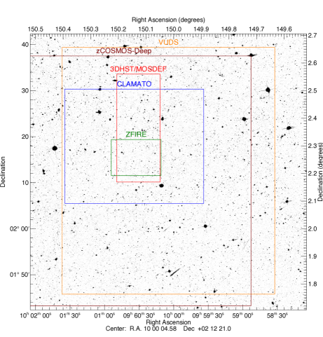
Figure 1: CLAMATO in context: the background image is the Hubble Space Telescope ACS F814W mosaic (Koekemoer et al., 2007) of the central regions in the COSMOS field, with the footprint of the CLAMATO Ly$\alpha$ absorption tomographic map indicated in blue. Also shown are the approximate footprints for other spectroscopic redshift surveys that probe similar redshifts, such as 3D-HST (Momcheva et al., 2016) and MOSDEF (Kriek et al., 2015) in red, zCOSMOS-Deep (Lilly et al., 2007) in brown, VUDS (Le Fèvre et al., 2015) in orange, and ZFIRE (Nanayakkara et al., 2016) in green.

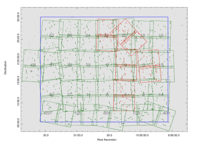
Figure 2: Slits and footprints of the 32 Keck-I/LRIS slitmasks observed in CLAMATO, overlaid on top of the deep Hubble Space Telescope ACS F814W mosaic of the COSMOS field (Koekemoer et al., 2007). The blue box indicates the footprint of the reconstructed tomographic map from the $2.15<z<2.55$ Ly$\alpha$ forestbsorption. Most of the slitmasks were designed to achieve a uniform survey layer (dark green), while several were ‘special’ slitmasks (red) designed to obtain additional lines of sight in specific regions. The numbers in grey are the field numbers we assigned to the slitmasks.

2.1 Source Catalogs

The CLAMATO survey is designed to maximize the areal density and homogeneity of background sources in the COSMOS field (Scoville et al., 2007) that could probe the Ly$\alpha$ forest absorption at $z\sim 2-2.5$. To achieve this, we exploit the high-quality multi-wavelength photometric redshifts (Ilbert et al., 2009; Laigle et al., 2016; Davidzon et al., 2017) available in the field, and also retarget spectroscopically-confirmed objects in the zCOSMOS-Deep (Lilly et al., 2007) and VUDS (Le Fèvre et al., 2015) surveys.

As a first step, we assembled a raw master catalog containing all objects $g<25.2$ within a redshift range that allows observations of the Ly$\alpha$ forest in the target volume, corresponding to objects with $2.0<z<3.5$. We began with a compilation of spectroscopic sources in the COSMOS field (Salvato et al, in prep), which, at our redshifts of interests, are primarily from the zCOSMOS-Deep (Lilly et al., 2007) and VUDS (Le Fèvre et al., 2015) catalogs. This was then further supplemented with the MOSDEF spectroscopic survey (Kriek et al., 2015), ZFIRE spectroscopic survey (Nanayakkara et al., 2016), and 3D-HST grism redshift catalog (Momcheva et al., 2016).

We then further filled in our master catalog using objects with only photometric redshifts. This initially used the $I$-band selected photometric redshift catalog from Ilbert et al. (2009), but prior to the 2017 observing season this was supplemented by near-IR selected photometric redshifts (Laigle et al., 2016; Davidzon et al., 2017) that yield more accurate redshift estimates.

2.2 Selection Algorithm

The target selection algorithm was carried out in two steps; initial prioritization of possible targets, followed by design of the individual slit-masks. Due to the spatial constraints of each LRIS slit-mask, only a subset of the possible targets could be manifested as slits.

For target prioritization, we fed the photometric/spectroscopic catalogs described in Section 2.1 into an algorithm designed to homogeneously probe our target area at $z\sim 2.3$. In order to ensure sufficient spatial resolution within a finite volume at $z\sim 2.3$ along the line of sight, we run our algorithm at two separate redshifts – $z_{\alpha}=2.25$ and $2.45$ – and then merged the target lists. Our algorithm divides the survey footprint into square cells of our desired sight-line separation, 2.75 arc-minutes on each side. In each cell, we select candidate background sources that could theoretically probe the forest at $z_{\alpha}$ in the restframe $1040\,\mathrm{\AA}<\lambda<1216\,\mathrm{\AA}$, i.e. between the Ly$\alpha$ and Ly$\beta$ transitions, corresponding to redshifts $(1+z_{\alpha})1216/1195-1<z_{\mathrm{bg}}<(1+z_{\alpha})1216/1040-1$. We then give the highest priority to “bright” sources with $g<[24.2,24.4]$ at $z_{\alpha}=[2.25,2.45]$ which have confirmed spectroscopic redshifts, and down-prioritize objects with only photometric redshifts or at fainter magnitudes.

Due to slit-packing constraints, the algorithm deprioritizes relatively bright sources if another, brighter, high-confidence target is within the same cell, while fainter or photometric redshift targets might receive relatively high priority in the absence of other suitable background sources within its 2.75 arc-minute cell. Due to the possibility that slit collisions from targets in other cells might clobber the highest-priority source within a given cell, the algorithm selected multiple sources per cell (with decreasing priority) where available. This procedure selected targets as faint as $g=25.3$ in regions lacking brighter candidates, but such faint targets were assigned a commensurately low priority.

The initial selection of sources, and their priority rankings from this algorithm, were then fed into the AUTOSLIT3 software in order to design LRIS slitmasks. The initial slit assignment was automatically carried out by AUTOSLIT3 based on the priorities assigned by the initial target selection algorithm, which we then manually refined to maximize the homogeneity of bright sources and the uniformity of redshift coverage within our desired $2\lesssim z_{\alpha}\lesssim 2.5$ redshift range. In each $7^{\prime}\times 5^{\prime}$ LRIS slitmask, we assigned $\sim 20-25$ science slits. Due to slit-packing constraints and the necessity of having at least 4 alignment stars within each slitmask, this limited us to only $\sim 80\%$ of the high-priority targets within our desired redshift range.

We designed a uniform set of slitmasks to cover our entire survey footprint (Figure 2), but also supplemented these with additional slitmasks — designed and observed in subsequent observing seasons after the initial pass— to increase sightline sampling in particular regions of interest (specifically the previously identified overdensities at $z\sim 2.5$, see section 5), or to make up for shortfalls in sightline density after the initial round of observations.

Over the 2019-2020 observing season, when it became apparent that further time allocations might not be forthcoming, we designed a row of slitmasks with horizontal orientations to try to ensure that the overall survey footprint would end up in a roughly rectangular shape. These horizontal slitmasks make up the bottom row of the survey footprint as seen in Figure 2.

3 Observations & Data Reduction

The CLAMATO observations were carried out using the LRIS spectrograph (Oke et al., 1995; Steidel et al., 2004) on the Keck-I telescope at Maunakea, Hawai’i. The observations described in this papers were carried out in 2014-2020 via a total time allocation of 20.5 nights, of which 18.5 nights were allocated by the University of California Time Allocation Committee (TAC) and 2 nights were from the Keck/Subaru exchange time given by the National Astronomical Observatory of Japan TAC. Out of this overall allocation, we achieved approximately 85hrs of on-sky integration.

CLAMATO focused on the LRIS blue channel, covering the range of $3700\,\mathrm{\AA}<\lambda<4400\,\mathrm{\AA}$ which corresponds to the restframe Ly$\alpha$ at $2.1\lesssim z_{\alpha}\lesssim 2.6$. We used the 600-line grism blazed at $4000\,\mathrm{\AA}$ in the blue channel which, with the $1^{\prime\prime}$ slitwidth we used, has a spectral resolution of $R\equiv\lambda/\Delta\lambda\approx 1100$. This corresponds to a FWHM of $\approx 4\,\mathrm{\AA}$ which translates to a line-of-sight spatial resolution of $3\,h^{-1}\,\mathrm{Mpc}$ at $z\sim 2.3$, comparable to the separation between our lines of sight. We use the red channel to assist in redshift determination and object identification.

Observations were conducted with a mean seeing of FWHM $\approx 0.7^{\prime\prime}$, and in $<0.8^{\prime\prime}$ seeing we typically exposed for a total of 7200s per typical survey slitmask. In suboptimal seeing we increased exposures up to a total of 14400s in order to attain approximately homogenous minimal signal-to-noise over the sky. For survey slitmasks designed to plug gaps, we integrated up to 19800s to gain sufficient signal-to-noise on fainter background sources and to deal with poor seeing conditions during those observations. Individual exposures in the blue channel were typically 1800s, while those in the red channel were only 860s to mitigate for the effects of cosmic ray hits on the red-channel’s thick fully-depleted CCDs (Rockosi et al., 2010).

The gathered data was reduced using the LowRedux routines from the XIDL software package. We performed initial flat-fielding, slit definition, and sky subtraction, and then co-added the 2D images of the individual exposures. We then traced the 1D spectra, additionally co-adding 1D spectra from different observing epochs which could not be co-added in 2D.

From the 32 unique slitmasks observed in the 2014-2020 CLAMATO campaign, we reduced and extracted 600 spectra from the blue channel, not including 19 spectra from unrelated ‘filler’ programs. The resulting spectra were then visually inspected and compared with common line transitions and spectral templates (particularly the Shapley et al. (2003) composite LBG template) to determine their redshift and classification type. Each spectra is then assigned a confidence flag with ranking of 0-4, where 0 denotes no attempt at identification due to a corrupted spectra or little source flux, 1 is a rough best guess, 2 is a low-confidence redshift, 3 is an object with reasonable enough classification certainty to be used for scientific results, while 4 is a high confidence redshift determined from multiple spectral features. Out of all the spectra, 393 spectra were determined to have $\geq$3 confidence rating of which 377 were at redshifts of $z>2$ (Figure 3). The faintest object of this category was a $g=25.29$ galaxy at $z=2.568$, although this was a Ly$\alpha$ emitter that could not be used for IGM tomography. These high-redshift, high confidence sources were classified into 359 galaxies ($95.5\%$) and 18 broad-line quasars (4.5%). Both populations are suitable for Ly$\alpha$ forest absorption surveys, but require different continuum fitting methods, as described in Lee et al. 2018b. We show a full table of extracted sources in Table 1, while examples of the spectra are shown in Figure 4. Nearly all sources with identified continuum were used for our end tomographic analysis, see § 4.

Table 1: CLAMATO Data Release 2 Redshift Catalog

ID#	$\alpha$ (J2000)	$\delta$ (J2000)	$g$-mag	$z_{\rm photo}$	$z_{\rm spec}$	Conf	Type	$t_{\rm exp}$ (s)	Tomo	$\mathrm{S/N_{Ly\alpha 1}}$	$\mathrm{S/N_{Ly\alpha 2}}$	$\mathrm{S/N_{Ly\alpha 3}}$
00762	10 01 00.905	+02 17 27.96	24.21	1.11	2.465	2	GAL	7200	N	$\cdots$	$\cdots$	$\cdots$
00765	10 01 00.297	+02 17 02.58	24.64	2.93	2.958	4	GAL	7200	Y	$\cdots$	$\cdots$	2.5
00767	10 01 14.934	+02 16 45.23	24.73	0.21	2.578	3	GAL	12600	Y	3.1	3.2	3.0
00771	10 01 06.870	+02 16 23.38	24.70	2.58	2.530	3	GAL	7200	Y	1.6	1.9	2.0
00780	10 01 14.359	+02 15 15.84	24.28	0.08	0.082	2	GAL	7200	N	$\cdots$	$\cdots$	$\cdots$
00783	10 01 07.412	+02 14 58.31	24.27	2.59	2.579	4	GAL	10200	Y	4.1	4.5	4.7
00784	10 01 15.952	+02 14 48.41	22.02	2.47	2.494	4	QSO	9000	Y	11.5	13.1	22.1
00785	10 01 05.138	+02 14 41.21	24.51	2.44	2.506	4	GAL	10200	Y	2.1	2.5	2.8
00787	10 01 21.083	+02 14 16.48	24.41	2.62	2.491	3	GAL	9000	N	0.8	1.0	1.1
00788	10 01 33.860	+02 14 25.19	24.24	2.62	2.738	3	GAL	9000	Y	$\cdots$	1.6	1.8

Note. — Table 1 is published in its entirety in the machine-readable format. A portion is shown here for guidance regarding its form and content.

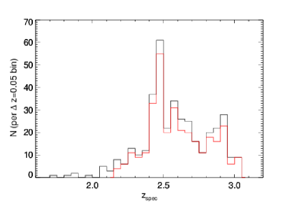
Figure 3: Redshift distribution of well-identified ($\geq 3$ confidence rating) spectra from CLAMATO, shown as the black histogram with redshift bins of $\Delta(z)=0.05$. The red histogram indicades background sources that were actually used to tomographicaly reconstruct the foreground Ly$\alpha$ forest at $2.05<z_{\alpha}<2.55$. These plot axes leave out 11 objects at $z<1.6$ and 1 object at $z>3.2$. Note that the spike at $z\sim 2.45$ is due to previously identified large over-density in this area (Diener et al., 2015; Chiang et al., 2015; Casey et al., 2015; Wang et al., 2016; Cucciati et al., 2018).

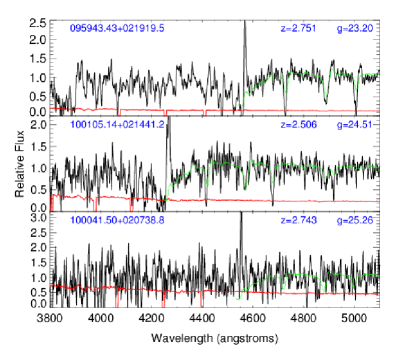
Figure 4: Examples of the reduced spectra used for IGM tomography in CLAMATO, showing, from top to bottom, galaxies with the brightest, median, and faintest $g$-magnitude. All three objects, coincidentally, exhibit clear Ly$\alpha$ emission. For clarity, the spectra have been smoothed with a 3-pixel tophat filter. The noise spectrum is shown in red, while redwards of Ly$\alpha$ we overplot the Shapley et al. (2003) LBG spectral template.

4 Tomographic Reconstructions

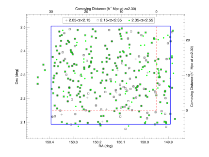
Figure 5: Points indicate the celestial positions of the Ly$\alpha$ forest lines of sight used to tomographically reconstruct the Ly$\alpha$ forest at $2.05<z<2.55$, with the blue rectangle showing the angular footprint adopted for the tomographic reconstruction — the pink dashed rectangle is the footprint from our previous data release (Lee et al., 2018b). The different symbols denote coverage over different redshift ranges. Some background sources have the correct redshift to cover large ranges of our targeted foreground redshift range and are therefore indicated by multiple symbols. The top and right-hand axes denote the coordinates of our tomographic map grid in units of transverse comoving distances, evaluated at the mean redshift of our tomographic map..

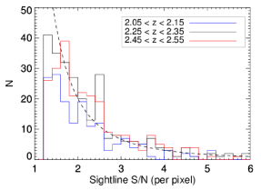
Figure 6: Distribution of the median sightline signal-to-noise within the Ly$\alpha$ forest, evaluated at several redshift bins within our map volume. A small number of higher signal-to-noise lines of sight have been left out by these plot axes. The dashed curve is a power-law with index of $-2.7$, which is a reasonable approximation for our signal-to-noise distribution.

In this section, we describe our methods for 3D tomographic reconstruction of the Ly$\alpha$ absorption seen in the spectra of our background selection. First, we describe the pre-processing of the reduced 1D spectra and setup of the tomographic reconstruction grid. Then, we describe the two methods we use for tomographic reconstruction: (i) Wiener-filtering of the transmitted Ly$\alpha$ flux, which was also used in our previous papers (e.g., Lee et al. 2014b, 2016, 2018b), and (ii) a constrained realization method to estimate the underlying matter density field (Horowitz et al., 2019b, 2020).

4.1 Data Preparation

We selected reduced spectra based on their continuum-to-noise ratio (CNR), defined as the value of the fitted continuum divided by the noise, within the Ly$\alpha$ forest absorption wavelengths for our tomographic analysis. We evaluate this ratio over three distinct absoprtion redshift windows: $2.05<z_{\alpha}<2.15$, $2.15<z_{\alpha}<2.35$ and $2.35<z_{\alpha}<2.55$. All high redshift objects with estimated confidence $\geq 3$ and $\langle\mathrm{CNR}\rangle\geq 1.2$ over any of these absorption windows were used in our tomographic reconstructions. This approach was fairly aggressive, selecting the vast majority of objects which had a confident redshift estimate (Figure 3), only excluding objects which had negligible continua. We show the sky positions of the selected lines of sight in Figure 5.

Figure 7: Effective area density of Lyman-$\alpha$ forest lines of sight over the redshift range of the CLAMATO tomographic reconstruction. The right axis labels the equivalent mean separation between lines of sight, $\langle d_{\perp}\rangle$, evaluated at $z=2.3$. The peak sightline density is $1056\,\deg^{-2}$ at $z_{\alpha}=2.28$, corresponding to $\langle d_{\perp}\rangle=2.07\,h^{-1}\,\mathrm{Mpc}$. Note that this estimate does not take into account the pixel masks in the spectra.

A total of 320 spectra from our observations fulfilled both the redshift criteria and signal-to-noise classification to contribute to our tomographic reconstruction of the Ly$\alpha$ forest within the target redshift range $2.05<z_{\alpha}<2.55$ in our footprint. We show the distribution of the estimated Ly$\alpha$ forest signal-to-noise in Figure 6 at different redshift ranges within our volume. We can model our signal-to-noise distribution with a power-law with index of $-2.7$, as done in Krolewski et al. (2017, 2018b). Based on the sky positions of the lines of sight, the transverse footprint of the tomographic reconstruction spans a comoving region of $30.1^{\prime}\times 24.8^{\prime}$ in the R.A. and declination dimensions, respectively (see Figure 5), centered at $10^{h}00^{m}34\fs 21,+02\arcdeg 17^{\prime}53.49^{\prime\prime}$ (J2000). This angular size is equivalent to a comoving scale of $30\,h^{-1}\,\mathrm{Mpc}\times 24\,h^{-1}\,\mathrm{Mpc}$ at $\langle z\rangle=2.30$. The mean sighline density is $\langle n_{\mathrm{los}}\rangle=856\,\mathrm{deg}^{-2}$ when averaged over the entire volume, equivalent to $\langle d_{\perp}\rangle=2.35\,h^{-1}\,\mathrm{Mpc}$ at $z=2.3$. At the two redshift extremes, $z=[2.05,2.55]$, we find an effective sightline density of $n_{\mathrm{los}}=[617,515]\,\mathrm{deg^{-2}}$, corresponding to an average transverse comoving seperation of $\langle d_{\perp}\rangle=[2.73,2.98]\,h^{-1}\,\mathrm{Mpc}$ (see Figure 7). Towards the middle of our redshift range we have the highest effective sight-line density, peaking at $1075\,\mathrm{deg^{-2}}$ at $z_{\alpha}=2.28$, equivalent to a transverse comoving separation of $\langle d_{\perp}\rangle=2.07\,h^{-1}\,\mathrm{Mpc}$. The overall sightline densities in the current CLAMATO data is marginally worse than in DR1, as the boost from the known galaxy overdensities at $z\sim 2.5$ in DR1 has been diluted by the increased map area.

The Ly$\alpha$ forest fluctuation at each pixel can be calculated from a given spectra with an estimated continuum, $C$. We divide the observed spectral flux density, $f$, by the mean Ly$\alpha$ forest transmitted flux, $\langle F\rangle(z)$, multiplied by the estimated continuum value;

$$\delta_{F}=\frac{f}{C\;\langle F\rangle(z)}-1.$$ (1)

We adopt the Faucher-Giguère et al. (2008) values for $\langle F\rangle(z)$, which are based on a sample of 86 high-resolution, high-signal-to-noise quasar spectra with absorption features extending well over this redshift range.

The intrinsic continua, $C$, of a quasar source is estimated based on a PCA-based mean-flux regulation (MF-PCA; e.g., Lee et al., 2012, 2013). For each spectrum, a continuum template is fitted to determine the correct shape for the QSO emission lines. A linear function is further fitted within the Ly$\alpha$ forest region (restframe $1041\,\mathrm{\AA}<\lambda<1185\,\mathrm{\AA}$ ) to ensure that the mean absorption is consistent with Faucher-Giguère et al. (2008). An analogous procedure is applied to the galaxy spectra, although assuming a broader Ly$\alpha$ forest range ($1040\,\mathrm{\AA}<\lambda<1195\,\mathrm{\AA}$) and fixing the continuum template from Berry et al. (2012). For galaxies we also explicitly remove intrinsic metal absorption lines at rest-frame N II $\lambda$1084, N I $\lambda$1134, C III $\lambda$1176, and Si II $\lambda\lambda 1190,1193$ using a $\pm 7.5\,\mathrm{\AA}$ (observed frame) mask. Uncertainties in the continuum estimation are propagated assuming a $\sim 10\%$ rms for the noisiest spectra ($\mathrm{S/N}\sim 2$ per pixel) and $\sim 4\%$ rms for the highest signal spectra ($\mathrm{S/N}\sim 10$ spectra); see Lee et al. (2012) for additional discussion.

We use the resulting flux pixel values, $\delta_{F}$, and associated noise uncertainties, $\sigma_{N}$, as inputs for our tomographic reconstructions. These extraced values are made publicly available and described in greater detail in Appendix A.

To perform our tomographic reconstructions, we define a cartesian grid in our footprint (Figure 5). To simplify our analysis, we assume a fixed Hubble parameter, $H(z)$, throughout our volume evaluated at $\langle z\rangle=2.30$. This is equivalent to setting a fixed differential comoving distance $\mathrm{d}\chi/\mathrm{d}z$, allowing for a direct correspondence between redshift segment length $\delta z$ and comoving distance $\delta\chi$. Our angular footprint of $30.1^{\prime}\times 24.8^{\prime}$ translates to a fixed comoving scale of $34\,h^{-1}\,\mathrm{Mpc}\times 28\,h^{-1}\,\mathrm{Mpc}$ at all redshifts in our map. Note that this will result in a slight variation of our smoothing kernel’s physical size from one side of our redshift range to the other. The alternative to this procedure would be use an evolving $H(z)$ over the volume, resulting in outward flared skewer positions relative to the comoving grid; this was found to negligible effect on the cosmic void analysis of Krolewski et al. (2017) while also breaking the one-to-one correspondence between $[x,y]$ and [RA, Dec], complicating analysis of the maps.

The angular footprint of this grid is $\sim 30\%$ larger than Lee et al. (2018a) and $4.5\times$ larger than that in Lee et al. (2016).

4.2 Wiener Filtering

To construct maps using the Ly$\alpha$ forest flux alone, we use a Wiener filtering (WF) scheme as done in Lee et al. (2018a). The basic algorithm is described in Pichon et al. (2001) and Caucci et al. (2008), and we use an implementation developed in Stark et al. (2015b). Other methods for direct flux reconstruction also exist including Cisewski et al. 2014 and Li et al. 2021b, which could be applicable depending on the end use of the maps. For WF, we solve for the Ly$\alpha$ forest flux fields:

$$\delta^{\mathrm{rec}}_{F}=\mathbf{C}_{\mathrm{MD}}\cdot(\mathbf{C}_{\mathrm{DD}}+\mathbf{N})^{-1}\cdot\delta_{F},$$ (2)

where $\mathbf{C}_{\mathrm{DD}}+\mathbf{N}$ and $\mathbf{C}_{\mathrm{MD}}$ are the data-data (with noise) and map-data covariances, respectively. We use a preconditioned conjugate gradient method to approximately solve the combination of matrix inversion and multiplication. For the noise covariance, we assume a diagonal form of $\mathbf{N}\equiv N_{ii}=\sigma_{N,i}^{2}$ which ignores sub-dominant errors from continuum mis-identification and other correlated errors. We impose a noise-floor of $\sigma_{N,i}\geq 0.2$ in order to not overly weight a small subset of high signal-to-noise lines of sight.

We also assume a Gaussian data-data covariance of the form $\mathbf{C}_{\mathrm{DD}}=\mathbf{C}_{\mathrm{MD}}=\mathbf{C(r_{1},r_{2})}$, following Caucci et al. (2008), and

$$\mathbf{C(r_{1},r_{2})}=\sigma_{F}^{2}\exp\left[-\frac{(\Delta r_{\parallel})^{2}}{2L^{2}_{\parallel}}\right]\exp\left[-\frac{(\Delta r_{\perp})^{2}}{2L^{2}_{\perp}}\right],$$ (3)

where $\Delta r_{\parallel}$ and $\Delta r_{\perp}$ are the distance between $\mathbf{r_{1}}$ and $\mathbf{r_{2}}$ along, and transverse to the line-of-sight, respectively. We adopt a transverse and line-of-sight correlation lengths of $L_{\perp}=2.5\,h^{-1}\,\mathrm{Mpc}$ and $L_{\parallel}=2.0\,h^{-1}\,\mathrm{Mpc}$, respectively, as well as a normalization of $\sigma^{2}_{F}=0.05$. This formulation of the covariance matrix and parameters were found in Stark et al. (2015b) to reasonably approximate the true covariance, have no explicit cosmological dependence, and provide accurate reconstructions on mock CLAMATO catalogs. The choices of $L_{\perp}$ and $L_{\parallel}$ are set by the average sight-line separation and the LOS spectral smoothing, respectively.

From the input map data of 84608 pixels, we perform a Wiener filter reconstruction using the Stark et al. (2015b) algorithm which solves the matrix inversion using a pre-conditioned conjugation gradient solver with a stopping tolerance of $10^{-3}$. The run-time for the entire volume was approximately 1000s using a single core of a Apple MacBook Pro laptop with 2.9 GHz Intel Core i5 processors and 16GB of RAM.

Our output grid is of size $68\times 56\times 876$ cells each $0.5\,h^{-1}\,\mathrm{Mpc}$ on a side with an effective smoothing scale of $\sim 2-3\,h^{-1}\,\mathrm{Mpc}$. The resulting map is publicly available for download as a binary file; see Appendix A for details.

4.3 Density Reconstructions and Cosmic Structure

In addition to the Wiener Filter flux reconstructions, we also reconstruct the underlying matter density field using the Tomographic Absorption Reconstruction and Density Inference Scheme (TARDIS, Horowitz et al. (2019b)). This method iteratively solves for the initial density field which gives rise to the observed structures through a forward modelling framework. Unlike the Wiener filtered reconstructions, this method solves for the underlying dark matter density fields, instead of the Ly$\alpha$ flux maps. This assumes an underlying $\Lambda$CDM cosmology and an analytical approximation to map from the evolved dark matter density to Ly$\alpha$ forest optical depth. One can view this process as iteratively solving for an intial density field, $\delta_{m}^{i}$, given the following forward operating steps;

$$\delta_{m}^{i}\xrightarrow[\textrm{N-Body }]{}(\delta_{m}^{z_{\alpha}},v_{m}^{z_{\alpha}})\xrightarrow[\textrm{FGPA}]{}(\tau_{\textrm{real}},v_{m}^{z_{\alpha}})\xrightarrow[\textrm{RSD}]{}\tau_{\textrm{red}}$$ (4)

where from the end redshift space optical depth, $\tau_{\textrm{red}}$, we select matching lines of sight as the CLAMATO Survey and iterate to find the density field that best matches the CLAMATO data. We assume the fluctuating Gunn-Peterson approximation, $\tau=A\exp{\delta_{m}^{\gamma}}$, for the hydrodynamical mapping from the matter density to Ly$\alpha$ flux, which was found to cause minimal decrease in cosmic structure recovery performance (Horowitz et al., 2020). For our N-Body solver, we use a particle mesh scheme as described in Modi et al. (2020). This resulting $\tau_{\textrm{red}}$ field is compared along each line of sight with the true data with a Gaussian likelihood weighted by the inferred pixel noise. All steps of our forward operator are differentiable, allowing fast optimization using first order based methods. In this case we use a Limited Memory Broyden–Fletcher–Goldfarb–Shanno (L-BFGS) solver which approximates the Hessian information via a truncated recursion relation from the previous update’s gradients.

In Horowitz et al. (2020), this framework was further extended to allow joint reconstruction of Ly$\alpha$ forest tomography with an overlapping galaxy sample. This work found a synergistic reconstruction effect, where Ly$\alpha$ forest absorption traced diffuse structures on large scales while galaxies were able to reconstruct the amplitudes of over-densities. As CLAMATO is located in the COSMOS field, there are a number of possible galaxy surveys to use for a joint reconstruction including ZFIRE, zCOSMOS, MOSDEF, etc. However, large scale structure reconstruction requires a well defined radial selection function which is difficult to determine in cases where the survey is designed to study a particular structure or galaxies of a certain sub-population (see Ata et al. (2020) for a discussion). We therefore use zCOSMOS (Lilly et al., 2007) as the corresponding galaxy sample to combine with the Ly$\alpha$ forest absorption, which comprises $\sim 45\%$ of all galaxies in the overlapping volume and has a well characterized selection function which we take from Ata et al. (2020).

In practice it would be computationally difficult to reconstruct the full volume at once due to the elongated geometry. We divide the volume into four overlapping cubic subvolumes of $L=128\,h^{-1}\,\mathrm{Mpc}$ each, with 15 $h^{-1}\,\mathrm{Mpc}$  overlap in the radial dimension. In addition we offset the data 10 $h^{-1}\,\mathrm{Mpc}$  into each reconstructed subvolume in order to minimize possible edge effects due to the simulations periodic boundary conditions. The reconstructed subvolumes are then pasted together, with a linear weighted averaging in the overlapping region. We have verified with mock catalogs that this pasting scheme does not introduce artifacts into the simulated volume nor decrease reconstruction quality in the overlap. Our reconstruction with this method takes approximately 30 minutes on a NVIDIA Tesla V100 PCle GPU card for the entire survey volume. We provide publicly our resulting reconstructed maps in numpy file format gridded in 1 $h^{-1}\,\mathrm{Mpc}$ cells.

As the reconstruction recovers directly the dark matter field in both real and redshift space, we can use these recovered fields for direct classification of the cosmic web environment. We use the pseudo-deformation tensor as described in Lee & White (2016); Krolewski et al. (2017) and based on work in Hahn et al. (2007); Bond et al. (1996); Forero-Romero et al. (2009). The pseudo-deformation tensor is defined as the Hessian of the gravitational potential, capturing the curvature information of the smoothed underlying density field. This tensor can be efficiently computed with known matter density in Fourier space, $\delta_{k}$, as

$$\tilde{D}_{ij}=\frac{k_{i}k_{j}}{k^{2}}\delta_{k}.$$ (5)

The eigenvectors of this tensor are related to the principle inflow or outflow directions depending on if the corresponding eigenvalue is positive or negative. The signature of the eigenvalues themselves can be used to classify the resulting cosmic structures as nodes, filaments, sheets, and voids (see Table 2).

	$\lambda_{1}$	$\lambda_{2}$	$\lambda_{3}$
Node	+	+	+
Filament	+	+	-
Sheet	+	-	-
Void	-	-	-

Table 2: Signature of the eigenvalues of the deformation tensor for structure classification.

5 Results

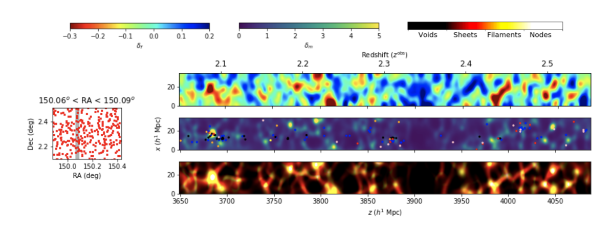
Figure 8: Wiener-filtered tomographic reconstructions of the Ly$\alpha$ forest absorption field, $\delta_{F}^{\mathrm{rec}}$, at $2.05<z_{\alpha}<2.55$ from the current CLAMATO data (color map), shown after smoothing with an isotropic $R=2\,h^{-1}\,\mathrm{Mpc}$ Gaussian kernel. Below the Wiener-filtered reconstruction, we show the inferred dark matter distribution from the TARDIS reconstruction and the inferred cosmic web classification, shown as a continuous color spectrum for the eigenvalues which can be mapped onto a discrete classification. Each color panel shows the field projected over a $2\,h^{-1}\,\mathrm{Mpc}$ R.A. slice, the position of which is denoted by the shaded region in the subpanels to the left that also show the sightline positions on the sky as red dots. The color convention for the absorption is such that red denotes overdensities while blue denotes underdensities. In the middle panel we show the overlapping galaxies within the slice; blue dots from MOSDEF, black dots from ZFIRE, pink dots from VUDS, orange dots from zCOSMOS-Deep, and red dots from CLAMATO. This sequence is continued in Figure 12, 13, and 14

We show an example slice of our reconstructed map via both Wiener Filtering and via forward model reconstruction in Figure 8. In addition to the reconstructed maps, we show a visualization of the cosmic structure as defined by the eigenvalues of the reconstructed matter deformation tensor, as well as coeval spectroscopically observed galaxies in the volume from different surveys. Each slab is projected over a thickness of $2\,h^{-1}\,\mathrm{Mpc}$, along right ascension, with the $y$-axis of each plot representing change in declination and the $z$ axis representing the redshift or line-of-sight dimension. For a clear comparison, we smooth all maps with a Gaussian kernel of $R=2\,h^{-1}\,\mathrm{Mpc}$, the approximate average sight-line spacing of the survey. We have also created a number of three dimensional renderings of our reconstructed flux field, dark matter density field, and inferred cosmic structures. These are available both in movie form (Figure 9) as well as a manipulable interactive figures (Figure 10).

There are a number of potential applications of these reconstructed maps to constrain intergalactic medium gas properties, galaxy formation and evolution, and cosmology. However, in this section we focus on a qualitative discussion of the structures recovered and will explore other applications in future work.

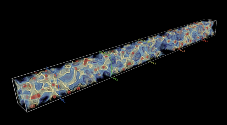
Figure 9: Still image from our 3D video visualization of the CLAMATO reconstructed cosmic web (smoothed with a $R=2\,h^{-1}\,\mathrm{Mpc}$ Gaussian kernel). Each cosmic structure classification is indicated with a different color; red for nodes, yellow for filaments, blue for sheets, and transparent for voids. These videos are available in the online journal and online at https://bit.ly/clamatoDR2.

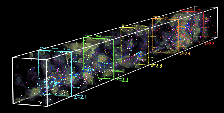
Figure 10: Three-dimensional rendering of the CLAMATO tomographic map, showing isodensity contours at $\delta_{F}^{\mathrm{rec}}=-0.260$, $-0.20$,$-0.14$,$-0.09$ along with coeval galaxy positions shown as dots color coded by galaxy survey (zCosmos: white, VUDS: purple, MOSDEF: blue, zfire: teal, CLAMATO: red). This figure is available online as an interactive figure (https://www2.mpia-hd.mpg.de/homes/tmueller/projects/clamato2020/clamato_vol.html). By left-clicking and moving the mouse, the viewpoint can be rotated, while the right-mouse button or scroll wheel can be used to zoom in or out; double left-clicking at any point in the map focuses the viewpoint there. A number of options are available to toggle different galaxy surveys and change the display of the flux iso-contours.

5.1 Large-Scale Structure Features

All of the visualizations show a rich cosmic web environment which is apparent in both the Wiener Filtered maps as well as the forward modelled reconstructions. We see a close correspondence between the reconstructed flux maps and the underlying galaxy surveys, with the significant caveat that all overlapping surveys have a non-uniform selection function along the line of sight and on the sky. Note that due to the varying selection functions and sky coverage of each survey, this galaxy sample is incomplete over our volume and it would be challenging to infer cosmic structures from galaxies alone (Horowitz et al., 2020).

Compared with Lee et al. (2018a), the expanded footprint allows the reconstruction of a complete picture of the cosmic web. With a transverse length of 35 $h^{-1}\,\mathrm{Mpc}$ and 30 $h^{-1}\,\mathrm{Mpc}$, we are able to completely capture filamentary structures spanning identified cosmic nodes within our survey area, as well as resolve sheet structures between filaments (see Fig. 9). In addition to filamentary structures, as in Lee et al. (2018a), we see apparent voids and (proto)clusters which have been previously discussed in past data releases in the same field (see Lee et al. 2015 and Krolewski et al. 2017) but now with increased sky coverage. We see that DR2 completely includes a number of previously identified galaxy protoclusters including the $z\sim 2.1$ galaxy protocluster first identified through the ZFOURGE medium-band photometric redshift survey (Spitler et al., 2012) and later confirmed with NIR spectroscopy (Nanayakkara et al., 2016).

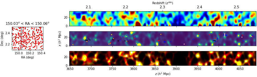
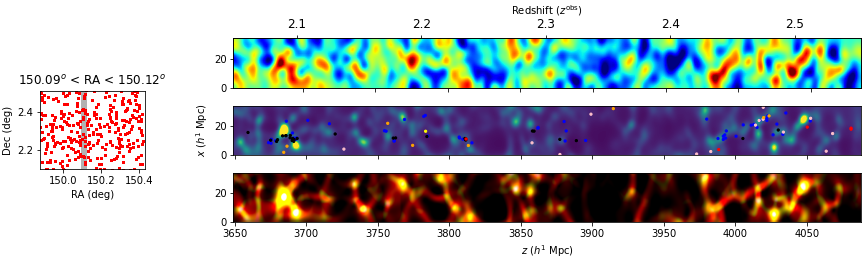
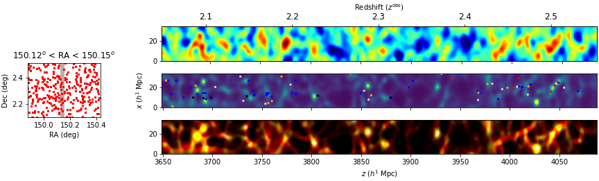
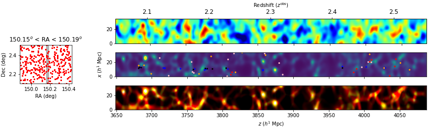
Figure 13: Continued from Figure 12.

In addition, the previously identified $z\approx 2.5$ overdensity comprised of the $z=2.44$ protocluster (Diener et al., 2015; Chiang et al., 2015), $z=2.47$ protocluster (Casey et al., 2015), and X-ray detected $z=2.51$ cluster (Wang et al., 2016; Cucciati et al., 2018), all appear to form a massive interconnected structure (see Figure 9 and 10) extending from $2.44<z<2.52$. While this structure was truncated by the survey geometry in Lee et al. (2018a), it does not appear to extend significantly beyond our current survey volume. The VUDS galaxy survey has been used to infer the general shape of this structure (see Cucciati et al. 2018), and we find our inferred Wiener filtered flux recovers a similar qualitative shape (see second panel of Figure 13). The exact correlation on small scales ($\sim 1$ h^-1 Mpc) between galaxy density and Ly$\alpha$ forest flux depends on the galaxy feedback model (Sorini et al., 2018). The late time fate of these mega-structures is of significant interest, with Wang et al. (2016) arguing that the $z=2.51$ overdensity, in itself, might collapse into a $2\times 10^{15}\,\mathrm{M}_{\odot}$. Using forward modelling techniques (Horowitz et al., 2019b, 2020; Ata et al., 2020) we will explore the late time fate of these structures in future works (Ata et al. in Prep).

5.2 Comparison of TARDIS and Wiener Filter Reconstruction

TARDIS is a fundamentally different approach that Wiener filter reconstruction since the resulting density fields are constrained to evolve from gravitational evolution and the hydrodynamical properties are determined via the Fluctuating Gunn Peterson Approximation, see Section 4.3. Substantial differences in the field reconstructed between these two methods could be indication of strong deviations from simple analytical approximations for the IGM flux-density relationship due to strong feedback within clusters environments (see, e.g., Kooistra et al. (2022)), or, e.g., possible galaxy quenching in overdense environments (Newman et al., 2022). In the case of mock catalogs which include hydrodynamical effects, TARDIS has shown to be still highly accurate in classification of cosmic structures at the resolution available to the CLAMATO survey (Horowitz et al., 2020). Also see Horowitz et al. (2019b) for a discussion of TARDIS reconstruction vs. Wiener Filtering in the absence of hydrodynamical effects.

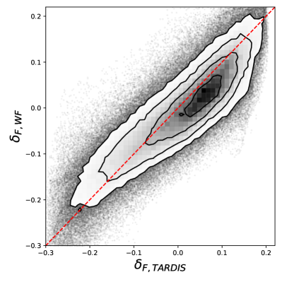
Figure 11: Relationship between the inferred flux from the TARDIS reconstruction and from the Wiener Filter reconstruction, both smoothed by 2 $h^{-1}\,\mathrm{Mpc}$. We find no significant biases between the two maps.

In addition to the slice-maps shown in Figures 12,13 14, we show the relationship between the inferred flux from TARDIS, calculated by performing an FGPA-transformation on the resulting density field, and that inferred from the Wiener filter approach in Figure 11. We find the results are largely consistent, with Pearson Correlation coefficient of 0.86. Further propagating this analysis to cosmic structure as defined by the eigenvalues of the deformation tensor, we find a Pearson Correlation coefficient of 0.83 between structures classified using the Wiener Filter and TARDIS, indicating similar cosmic structure reconstruction. Further investigation into the causes of the differences between these maps will be the focus of future work.

5.3 Three-dimensional Visualizations

Figure 9 shows a 3d visualization of the CLAMATO reconstructed cosmic web rendered using a self-developed software based on the Open Graphics Library (OpenGL) and the OpenGL Shading Language (GLSL) and implemented in C++.

Because our tomographic map consists only of scalar values, we can apply direct volume rendering where each density value is mapped to a particular color and opacity value via a transfer function. Then, a ray is generated for each image pixel and is sampled at regular intervals throughout the volume where the mapped RGBA values from the transfer function are composited in front-to-back order. For a smoother representation we use tricubic interpolation.

To highlight the cosmic structure classification, we use four Gaussians of nearly equal width to generate the transfer function. Sampling artifacts are reduced by making use of the pre-integration technique (Engel et al., 2001).

Finally, mesh and volume rendering are combined via two-pass rendering, where we first render color and depth of the grid mesh into two textures.In the second pass, the depth texture is used while the rays are integrated to check for intersections with the mesh.

Figure 10 shows a 3d visualization of the CLAMATO tomographic map also using direct volume rendering. This time the transfer function consists of four very thin Gaussians to represent isodensity contours. The interactive online version (https://www2.mpia-hd.mpg.de/homes/tmueller/projects/clamato2020/clamato_vol.html) is based on WebGL/threejs. The isodensity values as well as the corresponding opacities can be modified via slider controls in the online interface.

6 Conclusion

In this paper, we have described the second data release of the CLAMATO Survey, the first systematic attempt at implementing 3D Ly$\alpha$ forest reconstruction on several-Mpc scales using high area densities ($\sim 1000\,\deg^{-2}$) of background LBG and quasar spectra. With Keck-I LRIS observations of 23 multi-object slitmasks over $\sim 0.2\mathrm{deg}^{2}$ in the COSMOS field, we obtained 393 spectra with confident redshifts, of which 320 spectra were suitable for use in tomographic reconstruction in the target redshift range, $2.05<z_{\alpha}<2.55$ Ly$\alpha$ forest. This set of lines of sight has an average transverse seperation of only $\langle d_{\perp}\rangle=2.35\,h^{-1}\,\mathrm{Mpc}$, allowing us to create a three dimension tomographic map of the IGM and also infer the underlying dark matter density field. From this reconstructed map, we can identify for the first time the detailed cosmic web (including filaments and sheets) at high redshifts $z\sim 2.4$. We have made all catalogs, pixel data, and reconstructed maps available to the general public along with various analysis code (see Appendix A). With the extended volume of DR2, we are currently performing multiple additional analyses in this volume, including studying galaxy properties as a function of IGM and cosmic environment, analysis of the protoclusters within the volume, intrinsic alignments of galaxies with cosmic structure, constraints on hydrodynamical properties of the IGM from the various reconstructed maps, and cross-correlations between Ly$\alpha$ forest and coeval galaxies.

Going forward, the analysis done with the CLAMATO survey will serve as a test for planned and ongoing surveys over a wider sky region. The high redshift component of the Galaxy Evolution survey with the Prime Focus Spectrograph (PFS) on the 8.2m Subaru Telescope (Sugai et al., 2015) will perform an IGM tomographic analysis with similar sightline densities and noise properties as the CLAMATO survey over a $\sim 40\times$ larger cosmic volume. Beyond PFS, there are various additional facilities in different stages of planning ( e.g. the 11.25m Maunakea Spectroscopic Explorer (MSE, McConnachie et al., 2016b)) which will offer multiplex factors of several thousand over $\sim 1\deg^{2}$ fields-of-view allowing IGM tomography over tens or hundreds of square degrees. While the cosmological constraining power of the current CLAMATO survey is limited, with the expanded footprint of PFS or MSE there are potential applications to detect the weak-lensing of the Ly$\alpha$ forest (Metcalf et al., 2017) as well as perform full three dimensional Ly$\alpha$ forest power spectrum analysis (e.g., Font-Ribera et al., 2018; McDonald, 2003).

Appendix A Data Release

The second data release of the Keck-CLAMATO data is publicly available on Zenodo. These include the reduced spectra, continuum-normalized Ly$\alpha$ forest pixels used as the input for the tomographic reconstruction, the tomographic map of the $2.05<z<2.55$ IGM, and the inferred density field and cosmic structure from TARDIS.

There are a total of 600 reduced spectra in the data release, available in FITS format with the following headings:

• HDU0: Object spectral flux density, in units of $10^{-17}\mathrm{ergs\,s^{-1}\,cm^{-2}\,\mathrm{\AA}^{-1}}$

• HDU1: Noise standard deviation

• HDU2: Pixel Wavelengths in angstroms

On the data release webpage, we will provide an ASCII catalog that contains the information in Table 1 as well as the filenames for the spectra of each object. Note that the released spectrophotometry, especially in the red, might be unreliable.

We also will provide a binary file with the intermediate product of 84608 concatenated Ly$\alpha$ forest pixels (Equation 1) at $2.05<z_{\alpha}<2.55$ from the background sources that satisfy our redshift and signal-to-noise criteria. We will release the $\delta_{f}$ values and associated pixel noise as a function of the sky positions in $[x,y,z]$ on our tomographic map grid. The sky coordinates, $x$ and $y$, correspond to the transverse comoving distances in the R.A. and Declination directions, respectively. We choose an origin location of $[\alpha_{0},\delta_{0}]=[9^{h}59^{m}47\fs 999,+02\arcdeg 9^{\prime}0.00"]$ (J2000) or $[\alpha_{0},\delta_{0}]=[149.9500\arcdeg,2.1500\arcdeg]$. The $z$ coordinate corresponds to line-of-sight comoving distance relative to the origin redshift of $z_{\alpha}=2.05$. As mentioned in Section 4, we use a fixed conversion between redshift and the comoving distance in our volume. With our choice of cosmology, evaluated at $\langle z\rangle=2.30$, we have $\chi=3874.867\,h^{-1}\,\mathrm{Mpc}$ and $\mathrm{d}\chi/\mathrm{d}z=871.627\,h^{-1}\,\mathrm{Mpc}$. This intermediate binary file is the primary input used for the Wiener reconstruction and TARDIS algorithms to create the three dimensional tomographic maps.

The primary products are the binary files containing the IGM tomographic map, which spans comoving dimensions of $30\,h^{-1}\,\mathrm{Mpc}\times 24\,h^{-1}\,\mathrm{Mpc}\times 438\,h^{-1}\,\mathrm{Mpc}$ in the $[x,y,z]$ dimensions, respectively, with binning in units of 0.5 $h^{-1}\,\mathrm{Mpc}$. In addtion we make available our TARDIS reconstructions which cover the same volume but with binning in units of 1.0 $h^{-1}\,\mathrm{Mpc}$. For both products we provide both the direct tomographic reconstruction of the data, as well as a version which has been Gaussian-smoothed with a $\sigma=2\,h^{-1}\,\mathrm{Mpc}$ kernel; the latter is the version shown in the visualizations in Figures 9 and 10. We show slices of our various dataproducts in Figure 12, 13 and 14.

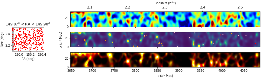
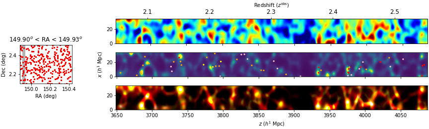
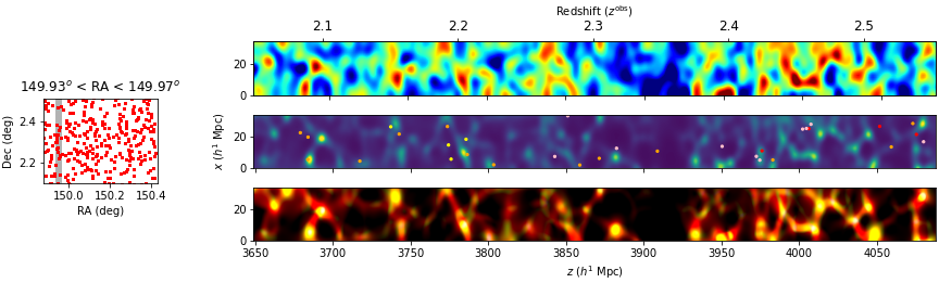
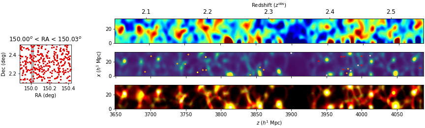
Figure 12: Wiener-filtered tomographic reconstructions of the Ly$\alpha$ forest absorption field, $\delta_{F}^{\mathrm{rec}}$, at $2.05<z_{\alpha}<2.55$ from the current CLAMATO data (color map), shown after smoothing with an isotropic $R=2\,h^{-1}\,\mathrm{Mpc}$ Gaussian kernel. Below the Wiener-filtered reconstruction, we show the inferred dark matter distribution from the TARDIS reconstruction and the inferred cosmic web classification, shown as a continuous color spectrum for the eigenvalues. Each color panel shows the field projected over a $2\,h^{-1}\,\mathrm{Mpc}$ Dec slice, the position of which is denoted by the shaded region in the subpanels to the left that also show the sightline positions on the sky as red dots. In the middle panel we show the overlapping galaxies within the slice; blue dots from MOSDEF, black dots from ZFIRE, pink dots from VUDS, orange dots from zCOSMOS-Deep, and red dots from CLAMATO. See Fig 8, continued on Fig 13 and 14

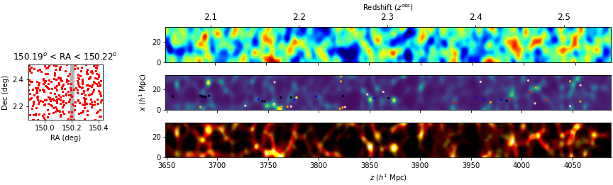
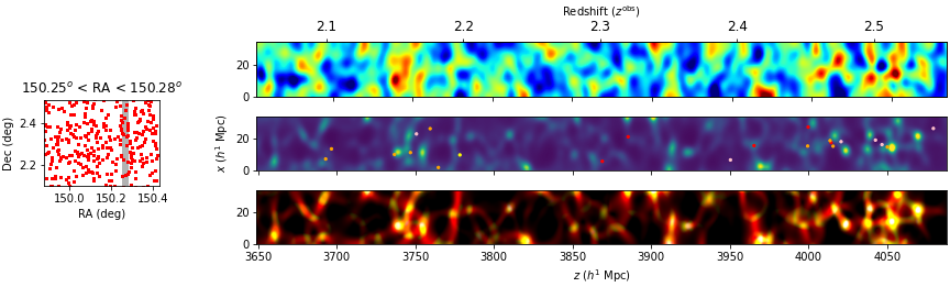
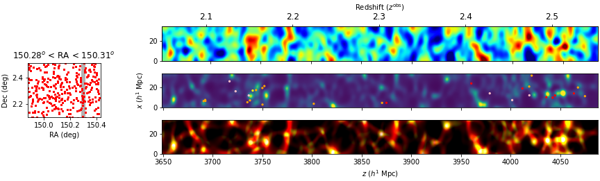
Figure 14: Continued from Figure 13.

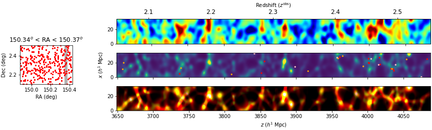
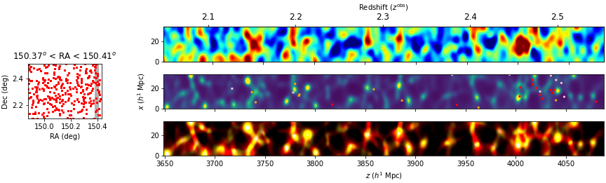
Figure 15: Continued from Figure 14.

References

- Alam et al. (2021) Alam, S., Aubert, M., Avila, S., et al. 2021, Phys. Rev. D, 103, 083533, doi: 10.1103/PhysRevD.103.083533
- Ata et al. (2020) Ata, M., Kitaura, F.-S., Lee, K.-G., et al. 2020, arXiv e-prints, arXiv:2004.11027. https://arxiv.org/abs/2004.11027
- Bautista et al. (2017) Bautista, J. E., Busca, N. G., Guy, J., et al. 2017, A&A, 603, A12, doi: 10.1051/0004-6361/201730533
- Berry et al. (2012) Berry, M., Gawiser, E., Guaita, L., et al. 2012, ApJ, 749, 4, doi: 10.1088/0004-637X/749/1/4
- Bond et al. (1996) Bond, J. R., Kofman, L., & Pogosyan, D. 1996, Nature, 380, 603, doi: 10.1038/380603a0
- Busca et al. (2013) Busca, N. G., Delubac, T., Rich, J., et al. 2013, A&A, 552, A96, doi: 10.1051/0004-6361/201220724
- Capak et al. (2007) Capak, P., Aussel, H., Ajiki, M., et al. 2007, ApJS, 172, 99, doi: 10.1086/519081
- Casey et al. (2015) Casey, C. M., Cooray, A., Capak, P., et al. 2015, ApJ, 808, L33, doi: 10.1088/2041-8205/808/2/L33
- Caucci et al. (2008) Caucci, S., Colombi, S., Pichon, C., et al. 2008, MNRAS, 386, 211, doi: 10.1111/j.1365-2966.2008.13016.x
- Chiang et al. (2015) Chiang, Y.-K., Overzier, R. A., Gebhardt, K., et al. 2015, ApJ, 808, 37, doi: 10.1088/0004-637X/808/1/37
- Cisewski et al. (2014) Cisewski, J., Croft, R. A. C., Freeman, P. E., et al. 2014, MNRAS, 440, 2599, doi: 10.1093/mnras/stu475
- Croft et al. (1998) Croft, R. A. C., Weinberg, D. H., Katz, N., & Hernquist, L. 1998, ApJ, 495, 44, doi: 10.1086/305289
- Cucciati et al. (2018) Cucciati, O., Lemaux, B. C., Zamorani, G., et al. 2018, A&A, 619, A49, doi: 10.1051/0004-6361/201833655
- Davidzon et al. (2017) Davidzon, I., Ilbert, O., Laigle, C., et al. 2017, ArXiv e-prints. https://arxiv.org/abs/1701.02734
- Dawson et al. (2013) Dawson, K. S., Schlegel, D. J., Ahn, C. P., et al. 2013, AJ, 145, 10, doi: 10.1088/0004-6256/145/1/10
- Delubac et al. (2015) Delubac, T., Bautista, J. E., Busca, N. G., et al. 2015, A&A, 574, A59, doi: 10.1051/0004-6361/201423969
- Diener et al. (2015) Diener, C., Lilly, S. J., Ledoux, C., et al. 2015, ApJ, 802, 31, doi: 10.1088/0004-637X/802/1/31
- du Mas des Bourboux et al. (2017) du Mas des Bourboux, H., Le Goff, J.-M., Blomqvist, M., et al. 2017, ArXiv e-prints. https://arxiv.org/abs/1708.02225
- Eisenstein et al. (2011) Eisenstein, D. J., Weinberg, D. H., Agol, E., et al. 2011, AJ, 142, 72, doi: 10.1088/0004-6256/142/3/72
- Engel et al. (2001) Engel, K., Kraus, M., & Ertl, T. 2001, in Proceedings of the ACM SIGGRAPH/EUROGRAPHICS Workshop on Graphics Hardware (New York, NY, USA: Association for Computing Machinery), 9–16, doi: 10.1145/383507.383515
- Faucher-Giguère et al. (2008) Faucher-Giguère, C., Prochaska, J. X., Lidz, A., Hernquist, L., & Zaldarriaga, M. 2008, ApJ, 681, 831, doi: 10.1086/588648
- Font-Ribera et al. (2014) Font-Ribera, A., McDonald, P., Mostek, N., et al. 2014, J. Cosmology Astropart. Phys, 5, 23, doi: 10.1088/1475-7516/2014/05/023
- Font-Ribera et al. (2018) Font-Ribera, A., McDonald, P., & Slosar, A. 2018, J. Cosmology Astropart. Phys, 2018, 003, doi: 10.1088/1475-7516/2018/01/003
- Forero-Romero et al. (2009) Forero-Romero, J. E., Hoffman, Y., Gottlöber, S., Klypin, A., & Yepes, G. 2009, MNRAS, 396, 1815, doi: 10.1111/j.1365-2966.2009.14885.x
- Gunn & Peterson (1965) Gunn, J. E., & Peterson, B. A. 1965, ApJ, 142, 1633, doi: 10.1086/148444
- Hahn et al. (2007) Hahn, O., Porciani, C., Carollo, C. M., & Dekel, A. 2007, MNRAS, 375, 489, doi: 10.1111/j.1365-2966.2006.11318.x
- Hammer et al. (2016) Hammer, F., Morris, S., Kaper, L., et al. 2016, in Proc. SPIE, Vol. 9908, Ground-based and Airborne Instrumentation for Astronomy VI, 990824, doi: 10.1117/12.2232427
- Horowitz et al. (2019a) Horowitz, B., Lee, K.-G., White, M., Krolewski, A., & Ata, M. 2019a, ApJ, 887, 61, doi: 10.3847/1538-4357/ab4d4c
- Horowitz et al. (2019b) —. 2019b, ApJ, 887, 61, doi: 10.3847/1538-4357/ab4d4c
- Horowitz et al. (2020) Horowitz, B., Zhang, B., Lee, K.-G., & Kooistra, R. 2020, arXiv e-prints, arXiv:2007.15994. https://arxiv.org/abs/2007.15994
- Horowitz et al. (2021) —. 2021, ApJ, 906, 110, doi: 10.3847/1538-4357/abca35
- Ilbert et al. (2009) Ilbert, O., Capak, P., Salvato, M., et al. 2009, ApJ, 690, 1236, doi: 10.1088/0004-637X/690/2/1236
- Japelj et al. (2019) Japelj, J., Laigle, C., Puech, M., et al. 2019, A&A, 632, A94, doi: 10.1051/0004-6361/201936048
- Kirkby et al. (2013) Kirkby, D., Margala, D., Slosar, A., et al. 2013, J. Cosmology Astropart. Phys, 3, 024, doi: 10.1088/1475-7516/2013/03/024
- Koekemoer et al. (2007) Koekemoer, A. M., Aussel, H., Calzetti, D., et al. 2007, ApJS, 172, 196, doi: 10.1086/520086
- Kooistra et al. (2022) Kooistra, R., Lee, K.-G., & Horowitz, B. 2022, arXiv e-prints, arXiv:2201.10169. https://arxiv.org/abs/2201.10169
- Kraljic et al. (2022) Kraljic, K., Laigle, C., Pichon, C., et al. 2022, MNRAS, 514, 1359, doi: 10.1093/mnras/stac1409
- Kriek et al. (2015) Kriek, M., Shapley, A. E., Reddy, N. A., et al. 2015, ApJS, 218, 15, doi: 10.1088/0067-0049/218/2/15
- Krolewski et al. (2017) Krolewski, A., Lee, K.-G., Lukić, Z., & White, M. 2017, ApJ, 837, 31, doi: 10.3847/1538-4357/837/1/31
- Krolewski et al. (2018a) Krolewski, A., Lee, K.-G., White, M., et al. 2018a, ApJ, 861, 60, doi: 10.3847/1538-4357/aac829
- Krolewski et al. (2018b) —. 2018b, ApJ, 861, 60, doi: 10.3847/1538-4357/aac829
- Laigle et al. (2016) Laigle, C., McCracken, H. J., Ilbert, O., et al. 2016, ApJS, 224, 24, doi: 10.3847/0067-0049/224/2/24
- Le Fèvre et al. (2015) Le Fèvre, O., Tasca, L. A. M., Cassata, P., et al. 2015, A&A, 576, A79, doi: 10.1051/0004-6361/201423829
- Lee et al. (2014a) Lee, K.-G., Hennawi, J. F., White, M., Croft, R. A. C., & Ozbek, M. 2014a, ApJ, 788, 49, doi: 10.1088/0004-637X/788/1/49
- Lee et al. (2012) Lee, K.-G., Suzuki, N., & Spergel, D. N. 2012, AJ, 143, 51, doi: 10.1088/0004-6256/143/2/51
- Lee & White (2016) Lee, K.-G., & White, M. 2016, ApJ, 831, 181, doi: 10.3847/0004-637X/831/2/181
- Lee et al. (2013) Lee, K.-G., Bailey, S., Bartsch, L. E., et al. 2013, AJ, 145, 69, doi: 10.1088/0004-6256/145/3/69
- Lee et al. (2014b) Lee, K.-G., Hennawi, J. F., Stark, C., et al. 2014b, ApJ, 795, L12, doi: 10.1088/2041-8205/795/1/L12
- Lee et al. (2015) Lee, K.-G., Hennawi, J. F., Spergel, D. N., et al. 2015, ApJ, 799, 196, doi: 10.1088/0004-637X/799/2/196
- Lee et al. (2016) Lee, K.-G., Hennawi, J. F., White, M., et al. 2016, ApJ, 817, 160, doi: 10.3847/0004-637X/817/2/160
- Lee et al. (2018a) Lee, K.-G., Krolewski, A., White, M., et al. 2018a, ApJS, 237, 31, doi: 10.3847/1538-4365/aace58
- Lee et al. (2018b) —. 2018b, ApJS, 237, 31, doi: 10.3847/1538-4365/aace58
- Li et al. (2021a) Li, Z., Horowitz, B., & Cai, Z. 2021a, arXiv e-prints, arXiv:2102.12306. https://arxiv.org/abs/2102.12306
- Li et al. (2021b) —. 2021b, ApJ, 916, 20, doi: 10.3847/1538-4357/ac044a
- Lilly et al. (2007) Lilly, S. J., Le Fèvre, O., Renzini, A., et al. 2007, ApJS, 172, 70, doi: 10.1086/516589
- McConnachie et al. (2016a) McConnachie, A., Babusiaux, C., Balogh, M., et al. 2016a, ArXiv e-prints. https://arxiv.org/abs/1606.00043
- McConnachie et al. (2016b) McConnachie, A. W., Babusiaux, C., Balogh, M., et al. 2016b, ArXiv e-prints. https://arxiv.org/abs/1606.00060
- McDonald (2003) McDonald, P. 2003, ApJ, 585, 34, doi: 10.1086/345945
- McDonald et al. (2006) McDonald, P., Seljak, U., Burles, S., et al. 2006, ApJS, 163, 80, doi: 10.1086/444361
- McQuinn (2016) McQuinn, M. 2016, ARA&A, 54, 313, doi: 10.1146/annurev-astro-082214-122355
- Metcalf et al. (2017) Metcalf, R. B., Croft, R. A. C., & Romeo, A. 2017, ArXiv e-prints. https://arxiv.org/abs/1706.08939
- Modi et al. (2020) Modi, C., Lanusse, F., & Seljak, U. 2020, arXiv e-prints, arXiv:2010.11847. https://arxiv.org/abs/2010.11847
- Momcheva et al. (2016) Momcheva, I. G., Brammer, G. B., van Dokkum, P. G., et al. 2016, ApJS, 225, 27, doi: 10.3847/0067-0049/225/2/27
- Momose et al. (2021) Momose, R., Shimasaku, K., Kashikawa, N., et al. 2021, ApJ, 909, 117, doi: 10.3847/1538-4357/abd2af
- Monzon et al. (2020) Monzon, J. S., Prochaska, J. X., Lee, K.-G., & Chisholm, J. 2020, AJ, 160, 37, doi: 10.3847/1538-3881/ab94c2
- Nagamine et al. (2020) Nagamine, K., Shimizu, I., Fujita, K., et al. 2020, arXiv e-prints, arXiv:2007.14253. https://arxiv.org/abs/2007.14253
- Nanayakkara et al. (2016) Nanayakkara, T., Glazebrook, K., Kacprzak, G. G., et al. 2016, ApJ, 828, 21, doi: 10.3847/0004-637X/828/1/21
- Newman et al. (2020) Newman, A. B., Rudie, G. C., Blanc, G. A., et al. 2020, ApJ, 891, 147, doi: 10.3847/1538-4357/ab75ee
- Newman et al. (2022) —. 2022, Nature, 606, 475, doi: 10.1038/s41586-022-04681-6
- Oke et al. (1995) Oke, J. B., Cohen, J. G., Carr, M., et al. 1995, PASP, 107, 375, doi: 10.1086/133562
- Palanque-Delabrouille et al. (2013) Palanque-Delabrouille, N., Magneville, C., Yèche, C., et al. 2013, A&A, 551, A29, doi: 10.1051/0004-6361/201220379
- Palanque-Delabrouille et al. (2016) —. 2016, A&A, 587, A41, doi: 10.1051/0004-6361/201527392
- Pichon et al. (2001) Pichon, C., Vergely, J. L., Rollinde, E., Colombi, S., & Petitjean, P. 2001, MNRAS, 326, 597, doi: 10.1046/j.1365-8711.2001.04595.x
- Pieri et al. (2016) Pieri, M. M., Bonoli, S., Chaves-Montero, J., et al. 2016, in SF2A-2016: Proceedings of the Annual meeting of the French Society of Astronomy and Astrophysics, ed. C. Reylé, J. Richard, L. Cambrésy, M. Deleuil, E. Pécontal, L. Tresse, & I. Vauglin, 259–266. https://arxiv.org/abs/1611.09388
- Ravoux et al. (2020) Ravoux, C., Armengaud, E., Walther, M., et al. 2020, J. Cosmology Astropart. Phys, 2020, 010, doi: 10.1088/1475-7516/2020/07/010
- Rockosi et al. (2010) Rockosi, C., Stover, R., Kibrick, R., et al. 2010, in Proc. SPIE, Vol. 7735, Ground-based and Airborne Instrumentation for Astronomy III, 77350R, doi: 10.1117/12.856818
- Schmidt et al. (2019) Schmidt, T. M., Hennawi, J. F., Lee, K.-G., et al. 2019, ApJ, 882, 165, doi: 10.3847/1538-4357/ab2fcb
- Scoville et al. (2007) Scoville, N., Aussel, H., Brusa, M., et al. 2007, ApJS, 172, 1, doi: 10.1086/516585
- Shapley et al. (2003) Shapley, A. E., Steidel, C. C., Pettini, M., & Adelberger, K. L. 2003, ApJ, 588, 65, doi: 10.1086/373922
- Siana et al. (2008) Siana, B., Polletta, M. d. C., Smith, H. E., et al. 2008, ApJ, 675, 49, doi: 10.1086/527025
- Skidmore et al. (2015) Skidmore, W., TMT International Science Development Teams, & Science Advisory Committee, T. 2015, Research in Astronomy and Astrophysics, 15, 1945, doi: 10.1088/1674-4527/15/12/001
- Slosar et al. (2011) Slosar, A., Font-Ribera, A., Pieri, M. M., et al. 2011, J. Cosmology Astropart. Phys, 9, 1, doi: 10.1088/1475-7516/2011/09/001
- Slosar et al. (2013) Slosar, A., Iršič, V., Kirkby, D., et al. 2013, J. Cosmology Astropart. Phys, 4, 26, doi: 10.1088/1475-7516/2013/04/026
- Sorini et al. (2018) Sorini, D., Oñorbe, J., Hennawi, J. F., & Lukić, Z. 2018, ApJ, 859, 125, doi: 10.3847/1538-4357/aabb52
- Spitler et al. (2012) Spitler, L. R., Labbé, I., Glazebrook, K., et al. 2012, ApJ, 748, L21, doi: 10.1088/2041-8205/748/2/L21
- Stark et al. (2015a) Stark, C. W., Font-Ribera, A., White, M., & Lee, K.-G. 2015a, MNRAS, 453, 4311, doi: 10.1093/mnras/stv1868
- Stark et al. (2015b) Stark, C. W., White, M., Lee, K.-G., & Hennawi, J. F. 2015b, MNRAS, 453, 311, doi: 10.1093/mnras/stv1620
- Steidel et al. (1996) Steidel, C. C., Giavalisco, M., Pettini, M., Dickinson, M., & Adelberger, K. L. 1996, ApJ, 462, L17, doi: 10.1086/310029
- Steidel et al. (2004) Steidel, C. C., Shapley, A. E., Pettini, M., et al. 2004, ApJ, 604, 534, doi: 10.1086/381960
- Sugai et al. (2015) Sugai, H., Tamura, N., Karoji, H., et al. 2015, Journal of Astronomical Telescopes, Instruments, and Systems, 1, 035001, doi: 10.1117/1.JATIS.1.3.035001
- Tie et al. (2019) Tie, S. S., Weinberg, D. H., Martini, P., et al. 2019, MNRAS, 487, 5346, doi: 10.1093/mnras/stz1632
- Viel et al. (2005) Viel, M., Lesgourgues, J., Haehnelt, M. G., Matarrese, S., & Riotto, A. 2005, Phys. Rev. D, 71, 063534, doi: 10.1103/PhysRevD.71.063534
- Wang et al. (2016) Wang, T., Elbaz, D., Daddi, E., et al. 2016, ApJ, 828, 56, doi: 10.3847/0004-637X/828/1/56