BIAS OF THE HUBBLE CONSTANT VALUE CAUSED BY ERRORS IN GALACTIC DISTANCE INDICATORS

Abstract

The bias in the determination of the Hubble parameter and the Hubble constant in the modern Universe is discussed. It could appear due to statistical processing of data on galaxies redshifts and estimated distances based on some statistical relations with limited accuracy. This causes a number of effects leading to either underestimation or overestimation of the Hubble parameter when using any methods of statistical processing, primarily the least squares method (LSM). The value of the Hubble constant is underestimated when processing a whole sample; when the sample is constrained by distance, especially when constrained from above, it is significantly overestimated due to data selection. The bias significantly exceeds the values of the error the Hubble constant calculated by the LSM formulae.

These effects are demonstrated both analytically and using Monte Carlo simulations, which introduce deviations in both velocities and estimated distances to the original dataset described by the Hubble law. The characteristics of the deviations are similar to real observations. Errors in estimated distances are up to $20\%$. They lead to the fact that when processing the same mock sample using LSM, it is possible to obtain an estimate of the Hubble constant from $96\%$ of the true value when processing the entire sample to $110\%$ when processing the subsample with distances limited from above.

The impact of these effects can lead to a bias in the Hubble constant obtained from real data and an overestimation of the accuracy of determining this value. This may call into question the accuracy of determining the Hubble constant and significantly reduce the tension between the values obtained from the observations in the early and modern Universe, which were actively discussed during the last year.

1 Introduction

The basis of modern cosmology is a homogeneous isotropic model, in which all points in the Universe and all directions are equivalent. Two details need clarification. It is possible that the Universe was anisotropic at the Big Bang time, but it became almost isotropic in the era of inflationary expansion in tiny fractions of a second and has been almost isotropic ever since. The temperature of the cosmic microwave background radiation is almost the same in all directions. This indicates a high degree of homogeneity and isotropy of the Universe during the epoch of recombination. However, as the Universe expanded, the fluctuations grew, e.g. of the density of the matter filling it. This led to the formation of a large-scale structure and the appearance of superclusters, voids, clusters, galaxies and stars. At present, we can talk about the homogeneity of the Universe only on very large spatial scales.

The rate of expansion of the Universe in such models is characterized by the time-dependent Hubble parameter $H$. It is defined as $H=\dot{a}/a$, where $a(t)$ is the scale factor and dot means the derivative with respect to cosmological time $t$. Its current value is called the Hubble constant and is denoted by $H_{0}$. Astronomers use the associated dimensionless quantity $h$, defined as $H_{0}=h\cdot 100$ km s^-1 Mpc^-1. With its help, Hubble velocities are easily converted into distances measured in Mpc $h^{-1}$. The modern estimate gives the value $h\approx 0.7$.

Most measurements of the Hubble parameter deal with distances, which are small by cosmological standards. They have small redshifts and relate to the late Universe. However, a few measurements relate to the early Universe, e.g. to the recombination era (redshift $z\approx 1100$). First of all, these are CMB data from Planck satellite [17] and data from Dark Energy Survey Year 1 clustering combined with data on weak lensing, baryon acoustic oscillations and Big Bang nucleosynthesis [1]. The data on primary nucleosynthesis deal with a process that took place in the first minutes of the existence of the Universe.

Estimations of the Hubble constant obtained by different methods are given in [22]. They are obtained from different observational data and based on different physical effects and its common constraints. The values given there, namely the estimation $H_{0}=67.4\pm 0.5$ km s^-1 Mpc^-1 in the recombination era and $H_{0}=73.3\pm 0.8$ km s^-1 Mpc^-1 in modern era are differ by 8%. The corresponding difference is at the level of $4\sigma-6\sigma$, which, according to [22], should be classified as something from a discrepancy or a problem to a crisis.

Numerous articles have tried to explain this difference in a variety of ways, including the introduction of new physical interactions in the early Universe. Naturally, the possible connection between the Hubble tension and the violation of the isotropy or homogeneity of the Universe was also considered. The review [4] contains links to 882 papers related to this issue. Some attempts to explain Hubble tension are discussed in [6,​ 20,​ 2]. According to [5] a systematic bias of $\sim$ 0.1 – 0.15 mag in the intercept of the Cepheid period-luminosity relations of SH0ES galaxies could resolves the Hubble tension. Note that in the paper [8] the value of $H_{0}=69.6\pm 0.8$ ($\pm 1.1\%$ stat) $\pm 1.7$ ($\pm 2.4\%$ sys) km s^-1 Mpc^-1 was find for the late Universe using the direct revised measurement of the tip of the red giant branch of the Large Magellanic Cloud. It agrees well with the ones for the early Universe.

I want to emphasize that the purpose of this work is neither to explain the differences in the estimates of $H_{0}$ for the early and late Universe due to the impact of some unaccounted factor nor to criticize any results obtained earlier. I want to demonstrate the pitfalls that always exist in data processing.

For this I am using the simplest example. The Monte Carlo method makes it easy to study the accuracy and precision of the estimates obtained; the use of the simplest least squares method with a single determinable parameter makes it possible not to consider the details of the complex analysis used in the processing of real data. I am not discussing Fisher matrices, possible abnormal distribution of deviations, discarding outliers, and other important processing details. My goal is to show that even in this simple case, the use of standard processing methods, but with different processing details, for example, the cut-off boundaries of the used subsamples, can give results that are quite different from each other. The formal application of statistical criteria could lead to the conclusion that there are significant differences in results of processing the same initial data set using the same method and the same procedure for its application.

I consider the issues of statistical processing of data on redshifts and estimating distances of galaxies in the modern Universe. I demonstrate that the differences in $H_{0}$ estimations could be explained by quite trivial reasons, such as the usage of statistical dependencies when estimating distances to galaxies.

To estimate distances to galaxies independently from redshifts astronomers have to use some distance indicators such as distance from Cepheid variables, the Tully-Fisher relation for spiral galaxies, the $D_{n}-\sigma$ or fundamental plane relations for elliptical galaxies, surface brightness fluctuations, brightest cluster galaxies, or tip of the red-giant branch. All of them are based of different statistical relations and provide distances with different accuracy.

The most precise of these statistical dependencies can only be used to estimate the distances to nearby galaxies, whose radial velocities exceed only slightly the characteristic speed of collective non-Hubble motions. For example, in the paper [18] luminosities of 75 Cepheids from the Milky Way were measured with errors of 1%. These data were used for calibration the distances. The estimate $H_{0}=73.0\pm 1.4$ km s^-1Mpc^-1, which differs by 4.2 $\sigma$ from the Planck results, was obtained using distance indicators based on these new data.

Tully-Fisher relation was generally considered to give the best distances to galaxies in the range required to define $H_{0}$ for some 20 years after its inception in [21]. It used a correlation for spiral galaxies between their luminosity and how fast they are rotating. The latter can be determined from the galaxy emission line widths. R.B. Tully wrote in his Scholarpedia article about the Tully-Fisher relation that at optimal passbands between 600 nm and 800 nm, its scatter is $\sim$0.35 magnitudes, equivalent to 17% uncertainty in distance. For other ranges or when using the dependence of the linear diameter on the emission line width, this uncertainty is bigger. This value is one of the parameters I use in Monte Carlo simulations. In modeling, I consider relative errors in determining the distance to individual galaxies (without using their redshift data) up to 20-30% based on the accuracy of the Tully-Fisher method. However, the accuracy of determining the Hubble constant is significantly higher due to the fact that statistical processing of a large array of data on galaxies is used.

Note that when estimating the distance from supernova Ia explosions, astronomers deal directly with the light curve and the spectrum from which the redshift can be determined. This was enough to discover the accelerated expansion of the Universe. Explosions can be considered the ‘‘standard candle’’ so beloved by cosmologists.

However, when determining the Hubble constant, the distance scale to them must be calibrated. This is done on the basis of data on the distances to galaxies in which a supernova explosion occurs, obtained from some of the criteria described above and retain all the systematic biases inherent in them. An overview of the methods used to determine the Hubble constant and construct a ladder of distances to distant extragalactic objects is given, in particular, in the review [9].

Whichever distance estimation method is used, one gets a set of estimated distances $R_{i}$ instead of true distances $r_{i}$ to galaxies. The difference between $R_{i}$ and $r_{i}$ are errors in estimating the distance to each galaxy we are talking about. They are not so small, since they accumulate all the errors inherent in all distance determination techniques used to estimate and calibrate the statistical dependence on all levels of the cosmic distance ladder. It is important that they increase with distance. Their impact leads to the bias in the value of the Hubble constant and its error could be significantly underestimated.

There are several sources of error in the determination of the Hubble parameter and the Hubble constant derived from it. One of them is the well-known bias, which arises because of errors in the argument of the function. It occurs during any statistical processing, including the least squares method (LSM) and the maximum likelihood estimation (MLE) for statistical data processing. It is discussed in the Section 2. The second one arises due to data selection effects when processing data from subsamples limited by distance obtain by indicators $R$. They are considered in the Section 3. I demonstrate their impact in subsections 2.4, 3.2 using the Monte Carlo method for mathematical modelling.

I also consider some potential sources of error that appeared to have no significant effect on the Hubble constant value. For example, in subsection 7.3 the influence of collective motions of galaxies aka cosmic streams is considered. Analysis show that it is not a source of errors when getting the $H_{0}$ value.

I considers and analyze some of the mathematical features of the used transformations in the subsection 7.1 in the Appendix. In the subsection 7.2 formulae for the are derived.

I sequentially consider several effects that affect the values of $H$ and $H_{0}$ obtained by processing observational data. I start with the simplest model, gradually adding additional factors related to the model used, sample completeness and processing details.

2 Underestimation of the Hubble constant caused by errors in galaxy distances

2.1 The simplest model of motion of galaxies and errors in distance and velocities measurements

Consider a sample of galaxies with distances $r_{i}$ and radial velocities $v_{i}$. At small redshifts $z\ll 1$ they are related by the Hubble law aka the Hubble-Lemaître law

$$v_{i}=Hr_{i},$$ (1)

where $H$ is the Hubble parameter. Therefore, one can exactly determine its value from any sample of $r_{i}$ and $v_{i}$. But the world is not so ideal and instead of this sample we have to process slightly different data.

It is possible to determine with great precision the actual measured radial velocity of each individual galaxy $V_{i}$ from its redshift. It is the sum of the velocities of its Hubble motion $v_{i}$ and the radial component of the peculiar motion of this galaxy. The last one is the sum of radial component of the collective non-Hubble motion of galaxies or galaxy flows and some random motion of this individual galaxy.

We start from the simplest model without collective non-Hubble motion. It does not consider significant variations in the density of matter existence in different regions of space. It is the reason for the appearance of non-Hubble flows of galaxies. When processing real data, we take into account these collective non-Hubble motions either by using their multipole expansion [15], or by directly simulating the influence of attractors and voids. In Section 7.3 I consider the influence of collective motion in the bulk motion approximation. However, let me remind you that my main goal is to show the pitfalls associated with statistical processing. And this is more clearly manifested when using the simplest models. So, I assume

$$V_{i}=v_{i}+\delta Vs_{i},$$ (2)

where $s_{i}$ is a random variable with normal distribution, zero mean and unit variance and $\delta V$ is the characteristic value of the random component of galaxy radial velocity.

We deal with a set of estimated distances to galaxies $R_{i}$ which are different from true ones $r_{i}$. One can assume that

$$R_{i}-r_{i}=ar_{i}p_{i},\;R_{i}=r_{i}(1+ap_{i}),$$ (3)

where $p_{i}$ is also a random variable with normal distribution, zero mean and unit variance and $a$ is the characteristic value of the relative error of the distance indicator we use.

Instead of (3) one can use

$$R_{i}-r_{i}=aR_{i}p_{i},\;R_{i}=r_{i}(1-ap_{i})^{-1}.$$ (4)

It is close to (3) for small errors in the distance estimation. In this case the error is a certain percent of $R_{i}$. I discuss the differences between these two types of noise (3) and (4) in the Sect. 7.1 and show that they are very different from a mathematical point of view. In addition to analytical consideration I use equations (2) and (3) or (4) to prepare a lot of mock samples for the Monte Carlo simulations. More details I discuss in the Section 2.3.

What type of relation can be expected from real astronomical observations? Statistical dependencies make it possible to estimate a certain parameter of the galaxy, which does not depend on the distance to it. Usually, this is its absolute luminosity $L$. For galaxies from the FGC and RFGC catalogues [10,​ 11] this is their linear diameter $D$. The errors of these values, if they are distributed over a gaussian, give the relation (3). To determine the distance, we need to use the flux from the galaxy, i.e. its apparent luminosity, or its angular diameter. Errors in these values, with their normal distribution, provide the relation (4). In general, we get a certain combination of relations (3) and (4).

I do not use this more general option. Relations (3) and (4) are quite enough for generating mock samples and derivation of formulae. After all, the purpose of our mathematical modelling is to demonstrate the effects and their rough estimate, and not an attempt to obtain particularly accurate estimates, taking into account all the nuances of real samples and methods of their processing.

2.2 Least squares data processing

I use the standard least squares method (LSM) formulae when processing mock samples data. LSM provides the optimal proportional relationship $V=AR$ between the $V_{i}$ and $R_{i}$ for the sample. If the statistical weights of the data points are the same, then the slope coefficient can be found by the formula

$$A=\frac{\sum_{i=1}^{N}V_{i}R_{i}}{\sum_{i=1}^{N}R_{i}^{2}}.$$ (5)

However, its slope coefficient would be equal to $A=kH$ instead of $H$ in (1). The factor $k$ characterizes the deviation of the values of the Hubble parameter and the Hubble constant obtained from true ones.

All odd plain central moments for a Gaussian distribution are zeroed. The mean values of $p_{i}^{n}$ are equal to $(n-1)!!$ if $n$ is even. Here $(n-1)!!$ denotes the double factorial, that is, the product of all odd numbers from $n-1$ to 1. The theoretical mean value of $k$ for the noise (2) and (3) is easy to estimate as follows

$$\begin{array}[]{l}k=\frac{\langle A\rangle}{H}=\bigg{\langle}\frac{\sum(Hr_{i}+\delta Vs_{i})r_{i}(1+ap_{i}))}{H\sum r_{i}^{2}(1+ap_{i})^{2}}\bigg{\rangle}\\ \approx\frac{\langle\sum r_{i}^{2}(1+ap_{i})\rangle}{\langle\sum r_{i}^{2}(1+ap_{i})^{2}\rangle}=\frac{1}{1+a^{2}}.\end{array}$$ (6)

Here the angle brackets mean averaging over the quantities $s_{i}$ and $p_{i}$. The average value of the numerator is $\sum Hr_{i}^{2}$. The average value of the denominator is $(1+a^{2})\sum Hr_{i}^{2}$. The average ratio slightly differs from the ratio of these average values due to the correlation between the terms with $p_{i}$ in the numerator and denominator, but for small $a$ this can be neglected.

The equation (5) provides the ratio of series for the noise (4).

$$\begin{array}[]{l}k=\bigg{\langle}\frac{\sum(Hr_{i}+\delta Vs_{i})r_{i}(1-ap_{i})^{-1}}{H\sum r_{i}^{2}(1-ap_{i})^{-2}}\bigg{\rangle}\\ \approx\frac{1+a^{2}+3a^{4}+15a^{6}+\ldots}{1+3a^{2}+15a^{4}+105a^{6}+\ldots}\leq 1.\end{array}$$ (7)

The numerator and the denominator contain the sum of two divergent series (11) and there are problems when applying the formula (5). This fact does not prevent us from using (5) to process mock samples.

This result is nothing new [3]. It is known that when using LSM for fitting by linear regression, errors in the velocities, i.e. ordinate of data points, lead to a scatter of the obtained values of the slope angle, but not to a bias. On the contrary, errors in distance estimate, i.e. the abscissa of data points, lead to a systematic underestimation of this angle. In the considered case, the underestimation is determined only by the parameter $a$. For $a=0.2$ we have an estimate for the mean value of the coefficient $k=0.96$, and for $a=0.3$ we have $k=0.92$. Note that this bias does not disappear at large sample size.

2.3 Demonstration of the effect using Monte Carlo simulations. Data and routine

It seems to me that direct demonstration of the effect is more convincing than theoretical estimates, especially if latter are not particularly simple. So I use the Monte Carlo (MC) method to demonstrate this effect and to clarify some important details.

I process 1000 mock samples. I do not use any real observational data, but I take ranges of distances close to the real sample for galaxies from the Flat Galaxies Catalogue (FGC) [10] and the Revised Flat Galaxies Catalogue (RFGC) [11]. I provide the results for the values of the parameters close to those obtained when processing real data, but I carry out calculations also for different parameter values, varying them within reasonable limits. In all cases the effects remain the same qualitatively.

Mock samples are generated as follows. The values $v_{i}$ were determined according to formula (1), corresponding to a preselected set of distances $r_{i}$. Then 1000 random sets of $V_{i}$ and $R_{i}$ were obtained from them, calculated by equations (2) and (3) or (4). I used the values $a=0.2$ and $\delta V=1000$ km s^-1 as a main choise. For details on how these parameters were obtained, see [15]. The values of the coefficient $k$ and its root-mean-square error $\Delta k$ are determined using the LSM formulae for each of these mock samples. In all cases, the average value of $k$ is 0.962 in accordance with (6).

To show the results obtained I use a dataset of 1402 galaxies located at a distance of $30h^{-1}$ Mpc to $100h^{-1}$ Mpc. Two galaxies are located at each distance interval of $0.1h^{-1}$ Mpc. Their Hubble velocities, calculated by (1), lie in the range from 3000 km s^-1 to 10000 km s^-1. Naturally, such a set has nothing to do with the real distribution of distances to galaxies. The impact of this distribution is discussed in Sec. 3.4. In the meantime, we are talking only about demonstrating the effect.

2.4 Demonstration of the effect using Monte Carlo simulations. Results

Fig. 1 shows one of the mock samples $V_{i}(R_{i})$ obtained by adding noise to this original dataset. It also shows a thick straight line on which the initial points $v_{i}(r_{i})$ lie and a straight dashed line drawn by the least squares method passing through the origin. The reason for underestimating the coefficient due to the abscissa changing is, in particular, the circled group of points on the right edge of the graph. In Fig. 1 we see a specific group of points for one of a mock sample. But for almost any mock sample, there is a similar group lying to the right of the straight line describing the Hubble law, which can be confused with outliers. The reason for this is discussed in Sec. 3.1 and shown in Fig. 3.

The slope was determined by formula (5), from which the $k$ values for each mock sample were determined. The distribution of $k$ values over different mock samples is close to a normal one. It is shown in Fig. 2. They was less than 1 for all 1000 mock samples and the mean value of the Hubble constant was underestimated by about $4\%$. The values of the LSM errors of $k$ are obtained in all cases using the standard LSM formula. Their typical value is $\Delta k\approx 0.1\%$. Thus, when processing any of mock samples, the underestimation of the value of the Hubble constant significantly exceeded the nominal error of this value, obtained using the standard data processing procedure.

Smaller average values of $k$ were obtained when using noise of the form (4). For $a=0.1$ MC simulations provide the value $\langle k\rangle=0.98$, for $a=0.15$ $\langle k\rangle=0.956$, for $a=0.2$ $\langle k\rangle=0.91$, for $a=0.25$ $\langle k\rangle=0.80$, and for $a=0.3$ $\langle k\rangle=0.58$. In this case, the impact of the effect under consideration increased.

Is it possible to obtain a more adequate result when processing, having an estimate of the values $a$ and $\delta V$? Let us try the maximum likelihood estimation (MLE). The formulae for calculating the slope of a straight line passing through the origin and fitting the $V_{i},R_{i}$ sample are derived in Sec. 7.2. The MLE at reasonable values of $a$ gives results even more deviating from the true ones than those obtained from the LSM. Using the condition (17) for processing the mock sample, shown in Fig. 1, one can get $k=0.93$. This sample was generated using (2) and (3) with $a=0.2$. The equation (19) provides the value $k=0.88$ for the mock sample prepared using (2) and (4) with $a=0.2$. So, MLE has no advantages over LSM in this case.

Therefore, in what follows, I will use only LSM for data processing and add noise in accordance with (3). More sophisticated methods of parameter determination and more accurate treatments of measurement error and noise sources will only complicate the presentation. Qualitative conclusions about effects are independent of these details.

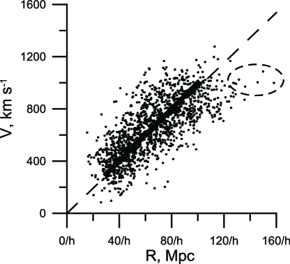
Fig. 1.: $V_{i}$ and $R_{i}$ data for one of the mock samples. The initial points $v_{i}(r_{i})$ lie on the thick straight line. The straight dashed line drawn by the LSM passing through the origin

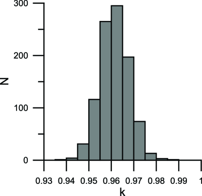
Fig. 2.: Histogram distribution of the $k$ parameter values for 1000 mock samples

3 Overestimation on the Hubble constant for subsamples with galaxy distances limitation

3.1 An impact of data selection when limiting the range of the distance indicator

Astronomers processing real observational data can get some $V(R)$ dependence similar to that shown in Fig. 1. They may have a rather natural idea to process not the entire sample, but its subsample obtained by limiting the range of $R$ variation from above or below, i.e. subsample with $R>R_{min}$, $R<R_{max}$ or $R_{min}<R<R_{max}$. And they have many reasons to do so.

At small distances the Hubble velocities do not exceed the velocities of random peculiar motions; it makes sense to exclude the influence of the Local Group, not to mention the natural limitation $R>0$, which can be violated, although very rarely, by noise of the type (3) at large random deviations $p_{i}$. At the far end of the sample there is an influence of the incompleteness of the sample or its asymmetry, in particular, due to the difference in observations in the two celestial hemispheres.

An astronomer dealing with the sample shown in Fig. 1 may decide to discard the data corresponding to the group of points surrounded by a dotted oval. One of the possible options is to process a subsample with $R_{max}=120h^{-1}$ Mpc.

However, by limiting the range of variation of the distance indicator $R$, one introduces some data selection into the subsamples. This leads to a statistical effect similar to the well-known Malmquist bias [12,​ 13].The influence of selection effects related to this has been examined in [14]. What is the mechanism of this selection? It is not difficult to illustrate it. Consider a subsample with upper-bounded distance indicators $R_{i}<R_{max}$ and a subsample in which a similar constraint is applied to the true distances $r_{i}<R_{max}$. In the latter, the slope of the dependence $v(r)$ is by definition equal to the Hubble parameter; when passing to the dependence $V(R)$ it is determined from (5).

The line in Fig. 3 corresponds to the Hubble law $v=Hr$. It contains the sample points $v_{i},r_{i}$, indicated by circles. Distance limits are shown with vertical dashed lines. The sample $V_{i},R_{i}$ is plotted on the same graph. Adding noise (3) shifts circles to the right or left, and noise (2) up or down. This corresponds to the arrows in Fig. 3. The squares show the positions of points with coordinates $v_{i},R_{i}$, i.e. an averaged position of the sample points $V_{i},R_{i}$.

If we consider two subsamples bounded by two vertical lines and fill in black the symbols of the points that fall there, then black circles will fall into the subsample with $R_{min}<r<R_{max}$, and the subsample with $R_{min}<R<R_{max}$ will get values shifted randomly up or down relative to the black squares. This is effect of non-Hubble motions. White circles and squares will be excluded from the corresponding subsamples. From the Fig. 3 it is easy to see how the centres of the possible location of the sample points $V_{i},R_{i}$ are located relative to the straight line.

Thus, the subsample with $R_{i}<R_{max}$ includes some black squares obtained by shifting white circles that are missing in the $r_{i}<R_{max}$ subsample, these are points with $R_{i}<R_{max}<r_{i}$. When adding noise according to formula (3), they shift to the left in Fig. 3. A noise like (2) shifts their position up or down, but on average they are above the straight line representing the Hubble law (1). In addition, some black circles that are present in the $r_{i}<R_{max}$ subset are discarded. They are shifted to the right so that $r_{i}<R_{max}<R_{i}$ and, on average, would be below the straight line.

So, in comparison with the sample $r_{i}<R_{max}$, the sample $R_{i}<R_{max}$ has additional points above the line $v=Hr$ and a number of points below it are excluded from the subsample. Therefore, the slope of the straight line approximating the points of this subsample is increased in comparison with the slope of the full sample (5). This is the effect of selection and it is caused by the statistical nature of distance indicators described by formula (3).

It is easy to show from similar reasoning that setting the lower limit of the distance indicators $R$ also leads to some selection. However, in this case the additional points are located mainly under the line and the discarded points are above it. In addition, in accordance with (3), the horizontal shifts near the lower boundary are significantly less than near the upper boundary; this weakens the influence of selection due to the establishment of the lower boundary.

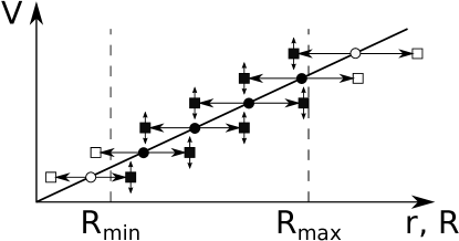
Fig. 3.: Explanation of the data selection mechanism caused by cropping the range of variation of the distance indicator to galaxies

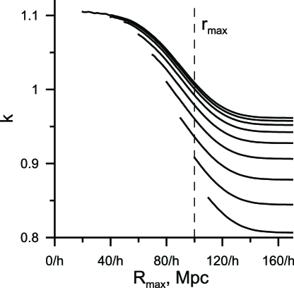
Fig. 4.: Dependence of $\langle k\rangle$ on $R_{max}$ at fixed $R_{min}$. The lines (from top to bottom) correspond to $R_{min}=20,\;30,\;40,\;50,\;60,\;70,\;80,\;90$ and $100h^{-1}$ Mpc

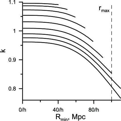
Fig. 5.: Dependence of $\langle k\rangle$ on $R_{min}$ at fixed $R_{max}$. The lines (from bottom to top) correspond to $R_{max}=\infty,\;120,\;110,\;100,\;90,\;80,\;70,\;60$ and $50h^{-1}$ Mpc

3.2 Monte Carlo simulations. Data and routine

I use the Monte Carlo simulations to produce a lot of $R_{i}$ and $V_{i}$ sets and then cut off all data outside the preselected limits of distance indicator to obtain mock subsamples. After processing them by LSM I get a set of $k$ coefficients according to (5) and calculate their mean value. This value is determined not only by the original sample, but also by the boundaries of the subsample.

What is it for? Each set of random deviations $p_{i},s_{i}$ gives a random mock sample, after cutting from above and below we get a set of mock subsamples. The values $k$ calculated for these subsamples are described by a distribution close to normal. It is characterised by its mean value $\langle k\rangle$ and the standard deviation $\sigma$. According to the central limit theorem, the mean value of $k$ obtained from $N$ subsamples is $\langle k\rangle$, and its root-mean-square deviation from the mean is close to $\sigma N^{-1/2}$. The error calculated by the LSM drops to zero with an increase in $N$, and can become significantly less than the deviation from the true value $k=1$. This could lead to a significant overestimation of the accuracy of the value obtained by the LSM, in particular, of the Hubble constant.

Naturally, we are primarily interested in the value $\langle k\rangle$. It depends on a number of parameters, primarily $a$. Obviously, for $a\to 0$ we have $\langle k\rangle\to 1$. The deviation from $\langle k\rangle=1$ monotonically increases with the growth of the parameter $a$. The value of $\langle k\rangle$ slightly depends on the distribution of the initial distances $r_{i}$. We will discuss this issue a little further when we consider the distribution of distances to galaxies in the realistic sample and the effect of its incompleteness.

In addition, the value of $\langle k\rangle$ is affected by details of generating the subsample such as the presence or absence of clipping at the top and bottom and the position of the boundaries of these clipping. I use the Monte Carlo method to study this dependence. It is much simpler and intuitive than complex analytical calculations.

The simplest initial sample is used: 991 galaxies with distances forming an arithmetic progression with an interval of $0.1h^{-1}$ Mpc. The distance to the most distant galaxy is $r_{max}=100h^{-1}$ Mpc, to the nearest one is $r_{min}=0.01r_{max}=1h^{-1}$ Mpc. In Figs. 4 and 5 the lower border lies slightly to the right of the ordinate axis, and the upper one is indicated on it by a vertical dashed line.

I have added random variations to the initial data using (1-3) with parameters $a=0.2$ and $\delta V=1000$ km s^-1. The subsamples are formed by simple cropping the same 1000 mock samples, which excludes the possibility of influencing the result by including or excluding individual points.

3.3 Monte Carlo simulations. Results

Figs. 4 and 5 show the $\langle k\rangle$ dependence on $R_{max}$ and $R_{min}$ values. Before discussing its details I want to emphasize that all points on them are obtained by processing different subsamples of the same mock samples using LSM. Nevertheless, the average $k$ values differ by ten percent or more. So, processing details are important.

Fig. 4 shows the mean $\langle k\rangle$ versus $R_{max}$ value for subsamples with different fixed values of $R_{min}$. The lines correspond to the different $R_{min}$ values. Top one corresponds to $R_{min}=20h^{-1}$ Mpc and almost coincides with the line drawn for subsample without cut-off from the bottom. Then there are lines with $R_{min}=30h^{-1}$ Mpc, $40h^{-1}$ Mpc, 50 $h^{-1}$ Mpc, $60h^{-1}$ Mpc, $70h^{-1}$ Mpc, $80h^{-1}$ Mpc, $90h^{-1}$ Mpc, and $100h^{-1}$ Mpc. I discard the leftmost edges of the curves, corresponding to subsamples with a small number of points by reason of a slight difference between $R_{max}$ and $R_{min}$.

Right parts of curves reach plateaus. This is because of the effect of selection associated with the upper bound of the subsample disappears at $R_{max}\gg r_{max}$. The height of the plateau depends on $R_{min}$, increasing as it decreases. At $R_{min}\ll r_{min}$, the influence of the selection associated with the lower cutoff limit disappears. In the absence of selection associated with both cuts, we get $\langle k\rangle=0.96$ in full accordance with (6). This corresponds to the height of the upper plateau. From Fig. 4 it can be seen that the value $\langle k\rangle$, obtained by the LSM, decreases monotonically with increasing either $R_{max}$ or $R_{min}$. This dependence is associated with an explanation of the reason for the selection effect and follows from Fig 3.

The left edges of the curves correspond to values at which the subsample still contains the minimum reasonable number of data points.

For clarity, Fig. 5 shows $\langle k\rangle$ as a function of $R_{min}$ for subsamples with different fixed $R_{max}$. Lines from bottom to top correspond to the values $R_{max}=\infty,120,110,100,90,80,70,60,50\;h^{-1}$ Mpc.

Let me remind you that the initial points before adding noise corresponded to the distances to galaxies from $r_{min}=30h^{-1}$ Mpc to $r_{max}=100h^{-1}$ Mpc. The lower limit lies to the left of the curves in Fig. 4 and the upper one is indicated on it by a vertical dashed line. The number of points to the left of $r_{min}$ is insignificant, so it depends little on $R_{min}<r_{min}$. Therefore, in Fig. 4 lines corresponding to $R_{min}=20h^{-1}$ Mpc and no clipping almost coincide and are represented by one upper curve. The $\langle k\rangle$ value decreases with increasing $R_{min}$ and constant $R_{max}$. This is caused by two reasons: a decrease in the number of points far from the edges and an increase in abscissa errors near the lower cutoff edge due to (3).

As $R_{max}$ increases, the number of points increases and the average value increases both for this reason and due to the influence of the above-described effect caused by the upper bound. At $R_{max}\gg r_{max}$, the number of points included in the subsample decreases greatly with a further increase in $R_{max}$ and the curve reaches a plateau. Its value depends on $R_{min}$ and at from $R_{min}\ll r_{min}$ tends to the value (6).

Figs. 4 and 6 show the results of LSM processing of the subsamples obtained by cutting $R_{max}$ and $R_{min}$. They also include some exotic variants with a strange choice of these values, which are unlikely to be used in real astronomical data processing. I want to return to the question of dependence of $\langle k\rangle$ on $a$ and consider a subsample with reasonable boundaries $R_{min}=30h^{-1}$ Mpc, $R_{max}=70h^{-1}$ Mpc. The value $\delta V=1000$ km s^-1 does not change, the initial $r_{i}$ set and other details are the same as for the previous calculations in this section. The plot of $\langle k\rangle$ versus $a$ is shown in Fig. 6. It can be seen from it that $k$ is overestimated by 2% at $a=0.1$ and by 5% at $a=0.16$. Thus, the introduction of the upper or/and lower bound significantly changes the obtained mean value of $k$.

In this case the distribution of $k$ is also close to normal as one can see in Fig. 7. Note that the histogram is based on the results of simulations with the same noise parameters, but for a different initial dataset. It contains more than 21400 points modeling galaxies, evenly distributed from $r_{min}=10h^{-1}$ Mpc to $r_{max}>1080h^{-1}$ Mpc. A subsample is chosen that is sufficiently distant from these boundary values, having $R_{min}=50h^{-1}$ Mpc $=5r_{min}$ and $R_{max}=90h^{-1}$ Mpc$<0.09r_{max}$ and containing over 800 mock data. The exact number for each simulation is determined by a set of random variables $p_{i}$ and ranges from 776 to 892 for 1000 mock samples used to construct Fig. 7. The scatter of values for different subsamples is greater than in Fig. 2. However, they are all not only greater than 1, but even greater than 1.07. The obtained distribution of values can be considered typical for subsamples with the lower and upper boundaries removed from the boundaries of the original distribution by distances.

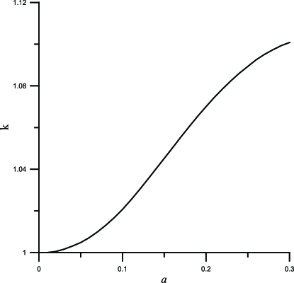
Fig. 6.: Dependence of $\langle k\rangle$ on $a$ for the subsample with $R_{min}=30h^{-1}$ Mpc $R_{max}=70h^{-1}$ Mpc

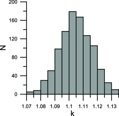
Fig. 7.: Histogram distribution of the $k$ parameter values for 1000 subsamples obtained from mock samples by distance limitation

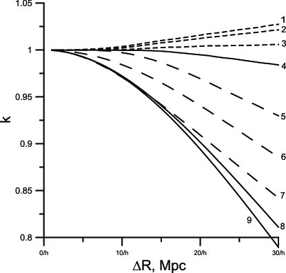
Fig. 8.: Dependence of $\langle k\rangle$ on $\Delta R$ with errors of distances in the form (8) for subsamples with different $R_{min}$ and $R_{max}$. The numbered curves 1-9 correspond to the following $R_{min}$ values: 0, 10, 20, 30, 30, 30, 30, 0 $h^{-1}$ Mpc and without cropping from the bottom. The $R_{max}$ values are 70, 70, 70, 70, 85, 100, 120 $h^{-1}$ Mpc and two curves without cropping from the top

Monte Carlo calculations confirm that selection caused by the upper limit $R_{max}$ leads to overestimating of $k$, while selection associated with the lower limit $R_{min}$ to it underestimating. The first effect is superior to the second with a reasonable choice of cutoff boundaries for errors of the form (3). The impact of data selection because of an upper limit on the distance indicator to the galaxy is several times greater than the effect previously described in Secs. 2.2 - 2.4. Note that the source of both is using of statistical relations to obtain a galaxy distance estimate independent of the redshift. The standard deviation of the mean for a sample of $N$ objects decreases with increasing $N$ in proportion to $N^{-1/2}$ and can become very small. But this average is biased and one deals with a classic example of an estimation with high precision and low accuracy.

3.4 Influence of distance distribution of galaxies

In the previous simulations I used the initial uniform distribution of galaxies over a certain interval of distances. This is not valid for real samples. At small distances the number of galaxies falling within the range of distances from $r$ to $r+dr$ is proportional to $r^{2}$ simply because they fall into the volume $4\pi r^{2}dr$. A number of far galaxies begins to decrease with distances due to the incompleteness of the sample, which simply does not include very distant galaxies. Naturally, a similar dependence is observed for the distribution of galaxies over the values of the distance indicators $R$.

I want to discuss the impact of both of these effects. They not only affect the effect caused by limiting the sample from above, but also lead to the appearance of another type of errors associated with data selection.

If we restrict the subsample by the condition $R<R_{max}$ and it has a high degree of completeness, then, compared to the uniform initial distribution of galaxies over distances, a large part of galaxies are located near the upper boundary and the influence of the selection discussed in the section is intensified. It is easy to verify this by applying the Monte Carlo method to a sample of 2815 galaxies distributed with a number proportional to $r^{2}$. At a distance of 30 $h^{-1}$ Mpc there are 36 galaxies, at a distance of 35 $h^{-1}$ Mpc there are 49 more galaxies, and so on up to a distance of 100 $h^{-1}$ Mpc, where 400 galaxies are located. A random noise is added to this initial sample according to (2) and (3). The resulting 1000 mock samples are processed using LSM formulae. The results obtained are perfectly described by formula (4), as expected. For $a=0.2$, the average value is $k=0.96$, for $a=0.25$ $k=0.94$ and for $a=0.3$ on average $k=0.92$.

But the mean values of $k$ obtained for subsamples with $R_{max}=80h^{-1}$ Mpc turn out to be slightly larger than with the initial uniform distribution. For $a=0.15$ on average $k=1.08$, for $a=0.2$ $k=1.12$, for $a=0.25$ $k=1.16$ and for $a=0.3$ on average $k=1.19$.

With an increase in $R_{max}$, the influence of selection effects associated with sample incompleteness begins to take effect. As I mentioned in the Section 7.1, statistical dependencies allow us to estimate a certain quantity that does not depend on the distance to the galaxy, for example, its absolute luminosity or linear size. Then, the photometric distance or angular distance is obtained from it and observable quantities such as apparent magnitude or angular dimensions.

Since the dependencies are statistical, the luminosity or size of each individual galaxy deviates from the average estimate. If they are larger or brighter, then we underestimate the distance to the galaxy, considering it closer than in reality. And if it is weaker or smaller in size, then we overestimate the distance. In formula (3) this corresponds to negative and positive values of $p_{i}$, and in Fig. 3 to left and right shifts.

However, a brighter or larger galaxy is more likely to get into the sample than a faint small galaxy. Therefore, it should be expected that the number of galaxies shifted to the right will exceed the number of galaxies shifted to the left. The distribution of the $p_{i}$ values for the galaxies included in it will still be random, but it will not only be different from Gaussian, but also have a nonzero mean. As a result, the sample will include fewer galaxies lying above the line $V=HR$ and more ones lying below it. This will lead to an additional underestimation of the value of $k$ obtained by processing the data using the LSM versus complete sample.

As one can see, this selection acts in exactly the opposite way than the selection associated with the consideration of subsamples limited by distance. Note that both in deriving (6) and in simulations, I did not consider the influence of this effect in the Sect. 3.1, assuming that a galaxy can move in the $V,R$ plane relative to its true position, but not disappear from the sample.

4 Impact of distance-dependent and independent errors

For completeness, I also performed similar simulations with the distance estimation errors in the form

$$R_{i}=r_{i}+\Delta Rp_{i}.$$ (8)

In this case the distribution of deviations in the estimation of the distance does not depend on this distance, in contrast to the previously considered errors of the form (3) or (6). So, the effect associated with the difference in magnitude of errors for nearby and distant galaxies disappears. But this does not mean that there is no difference between the effect of cutoffs at the upper bound of the subsample, described by $R_{max}$, and at the lower, characterized by $R_{min}$. The reason is that we fit the data with a relationship in the form (1), i.e. a line through the origin. Naturally, the origin is nearer to a lower border.

I apply the Monte Carlo method to the initial dataset with data for 991 mock galaxies, which is similar to the one used in the previous section and apply noise to it 1000 times. I add random errors of the form (2) with the same value $\delta V=1000$ km s^-1 and the form (8) with different values of $\Delta R$. A bias also exists in this case.

I do not show graphs similar to Fig. 4 or 5, and go straight to the analogue of Fig. 6, i.e. dependencies of $\langle k\rangle$ on $\Delta R$ for various cutting of a noisy sample. In this Fig. 8, solid lines depict three natural choices of the values $R_{max}$ and $R_{min}$. These curves are indicated by the numbers 9, 8 and 4. Curve 9 corresponds to the absence of any clipping. For it, from (5) by a method similar to (6), it is easy to obtain a theoretical estimate

$$\begin{array}[]{l}k=\frac{\langle A\rangle}{H}=\bigg{\langle}\frac{\sum(Hr_{i}+\delta Vs_{i})(r_{i}+\Delta Rp_{i}))}{H\sum(r_{i}+\Delta Rp_{i})^{2}}\bigg{\rangle}\\ \approx\bigg{(}1+\frac{\Delta R^{2}}{U^{2}}\bigg{)}^{-1}.\end{array}$$ (9)

Here $U^{2}=\langle r_{i}^{2}\rangle$. For the initial sample I used for MC simulations $U\approx 60h^{-1}$ Mpc.

However, due to errors, there could be some galaxies with distance estimates $R_{i}<0$. It is hard to imagine that they are not discarded during processing. Therefore, I also considered a subsample with $R_{min}=0$ without cutting from the top. It is easy to understand that the obtained values of $k$ will be larger for it than (9) due to the fact that points in the region $R<0$ provide negative contribution to the numerator (9) on average. By discarding them, we increase $k$ and decrease its deviation from 1. This subsample corresponds to the curve 8 in Fig. 8.

I use the bounds $R_{min}=30h^{-1}$ Mpc, $R_{max}=70h^{-1}$ Mpc, i.e. those that were used to calculate the graph in Fig. 6, as the third natural choice (the curve 4 in Fig. 8). One can see that in this case the deviation of $k$ from 1 is significantly less than for the full sample, for which it is well described by equation (9). This demonstrates that the influence of data selection is significant even for errors of the type (8). Comparing Fig. 8 and Fig. 6, one can see that errors of the form (3) lead to an overestimation of $k$, and those of the form (8) to its underestimation at the same subsample bounds.

Some additional lines are drawn in Fig. 8 to show how the values of $R_{max}$ and $R_{min}$ affect $k$. The dashed lines 1-3 correspond to different values of $R_{max}$ with the same value of $R_{min}=30h^{-1}$ Mpc and the lines 5-7 with longer dashes correspond to different values of $R_{min}\geq 0$ with the same value of $R_{max}=70h^{-1}$ Mpc. For curves 4, 3, 2, 1 $R_{min}=30,20,10,0\;h^{-1}$ Mpc. It can be seen that with a decrease in $R_{min}$, the average $k$ increases and underestimation is replaced by overestimation. Lines 4, 5, 6, 7 correspond to the upper bounds with $R_{max}=70,85,100,120\;h^{-1}$ Mpc, and the line for a subsample without upper distance limitation ($R_{max}=\infty$) absent on the chart is slightly above curve 9. It can be seen that an increase in $R_{max}$ leads to an increase in bias.

So, the bias is caused by a combination of three effects, namely the general underestimation (6) or (9) and the influence of selection when cutting off at the upper and lower boundaries of the subsample, the latter depend on $R_{max}$ and $R_{min}$. The ratio of them is different for errors (6) and (8).

Let’s try to compare the total bias for a reasonable choice of boundaries. For (3) with $a=0.2$ the standard deviation of the distances, i.e. a value similar to $\Delta R$ in (8) for a sample with $R_{min}=30h^{-1}$ Mpc, $R_{max}=70h^{-1}$ Mpc varies from $6h^{-1}$ Mpc at its lower boundary to $14h^{-1}$ Mpc at its upper boundary. The bias is much less than 1% for curve 4 and $\leq 5\%$ for all curves in Fig. 8 for $\Delta R\leq 14h^{-1}$ Mpc. It can be seen that errors of the form (3) provide a larger bias and more often lead to an overestimation of the value of $k$ than that of the form (8).

This is an important detail that makes it possible to quite successfully apply the LSM in the case when the random error of the abscissa is constant. It is not met in the case of determining the Hubble parameter and the Hubble constant, when as the distance to galaxy increases, so does the error in its determination.

5 Bias correction

Naturally, astronomers usually do not process observational data using standard software packages. They try to minimize possible bias by correction. They take into account factors that directly affect the measured quantities, such as extinction, or the aperture of a telescope. The data is corrected to reduce the influence of known physical effects, for example, the change in luminosity depending on the redshift or the curvature of space-time is taken into account. The influence of statistical factors is also taken into account, for example, a correction for Malquist bias.

The effect described in Sec. 2.2 can be corrected by applying the so-called ‘‘correction for attenuation’’ which would multiple $A$ by $1+a^{2}$, assuming that $a$ is known. However, you need to know the error distribution and all its parameters for effective bias-correction. In real measurements, deviations are usually caused by several factors. In the Section 2.1 I gave an example of errors in estimating the distance from the Tully-Fisher dependence in the ‘‘linear diameter — the emission line-width’’ version, where errors of the method itself, as well as errors of measurements of the angular dimensions and line width, led to different dependences of errors on distance.

It is difficult to take into account and compensate for the effect of cut-off of the sample and its incompleteness without knowing the distribution of objects in the sample. So we can correct the value of the determined quantity rather ambiguously. They can be affected during processing.

A well-known example of such an influence is provided by experiments on measuring the charge of an electron. R.A. Millikan was awarded the Nobel Prize in Physics in 1923 ‘‘for his work on the elementary charge of electricity and on the photoelectric effect’’. This is how this phenomenon is described in R. Feynman’s autobiographical book [7]: ‘‘One example: Millikan measured the charge on an electron by an experiment with falling oil drops, and got an answer which we now know not to be quite right. $<\cdots>$ It’s interesting to look at the history of measurements of the charge of the electron, after Millikan. If you plot them as a function of time, you find that one is a little bigger than Millikan’s, and the next one’s a little bit bigger than that, and the next one’s a little bit bigger than that, until finally they settle down to a number which is higher. $<\cdots>$ When they got a number that was too high above Millikan’s, they thought something must be wrong and they would look for and find a reason why something might be wrong. When they got a number closer to Millikan’s value they didn’t look so hard. And so they eliminated the numbers that were too far off, and did other things like that.’’

Note that the history of measuring the charge of an electron is somewhat similar to the definition of the Hubble constant in another aspect, too. A group of researchers from the University of Vienna, headed by F. Ehrenhaft, obtained the value of the electron charge less than that of Millikan, and for a long time there was a kind of ‘‘electron’s charge tension’’ in physics.

Thus, the correction can reduce, but not eliminate the influence of the discussed effects, and its application also can be a potential source of errors.

6 Discussion and conclusion

Two points can be drawn based on the results of this work. One is more general, the second refers to the Hubble tension. The first is associated with the result of data processing by any of the statistical methods used, starting with the LSM. The simplest simulations, which can be easily repeated by anyone show that there is a bias in defining simple quantities like a slope of a straight line running through the origin. It is associated with the error in estimating the quantity used as the abscissa. In our example these are the distances to galaxies. The result is a biased estimation which can be quite precise for a large sample, but not necessarily accurate. Bias in the estimation of a slope cannot be eliminated using more sophisticated statistical processing methods such as MLE.

Naturally, one can try to estimate it and introduce a correction for bias into the resulting value, similar to how a correction for Malmquist bias is introduced in some astronomical calculations. However, this is not easy to do. Bias is caused both by a general underestimation of the type (6) or (9), and by the influence of selection due to truncation of the sample or its incompleteness. The impact of a cutoff is different for the upper and lower sample boundaries. The total bias depends on the magnitude and distribution of the errors and on the distribution of both data points and errors over abscissa. It could lead either to underestimation or overestimation of the obtained slope, as can be seen in specific examples using the Monte Carlo method. All this greatly complicates the calculation of the correction that would compensate the impact of the effect under consideration.

These effects can significantly bias the value of the Hubble parameter as the slope of the straight line $v(r)$, determined from the redshift and the estimated distances to galaxies. Bias is quantitatively characterized by the deviation of the parameter $k$ defined as the ratio of the calculated value of the Hubble parameter to the true one from $k=1$. The influence of the abovementioned factors and some others, the influence of which turned out to be insignificant, is investigated both analytically and using the Monte Carlo method.

The value of the Hubble parameter and the Hubble constant obtained by LSM are underestimated in accordance with formulae (6) and (9). For typical precision distance indicators of $20\%-30\%$ the effect is about $4\%-8\%$. The error of the Hubble parameter obtained by the least squares formula is much less than bias. The distribution of the factor $k$ is close to normal. All $H$ values obtained by LSM are underestimated in all sets of 1000 simulations each.

If the mock sample is additionally cut off from above by the condition $R_{i}<R_{max}$ or/and from below by the condition $R_{i}>R_{min}$, this will lead to additional bias of the value of the Hubble parameter obtained by the LSM. The reason for this effect is explained in the Sect. 3. The results of MC simulations presented in Figs. 4, 5 and 8 show that the values of $k$ for subsamples obtained at different cutoffs of the same sample may differ significantly. The impact of the sample cutoff can not only exceed the influence of the aforementioned underestimation, but also leads to a general overestimation of the Hubble parameter value by about $8\%$ when using distance indicators with an accuracy of $20\%$. Note that the impact of the effect is highly dependent on the used model of the distance indicator error.

It can be assumed that the indicated effects can bias the value of the Hubble constant, determined by processing the data of real observations. Therefore, to check the adequacy of the processing methods applied in each specific case, it is advisable to carry out modeling using the Monte Carlo method by adding noise to the set of initially accurate data.

From a practical point of view, we are talking about the following sequence of actions. When processing data, one of the measured values is considered as a function of the rest of the measured values, considered as arguments of this function, and the set of parameters that we are calculating. Initially, the values and errors of all parameters are determined using conventional data processing. Then a mock sample is created. For this, the values of the arguments are taken from the sample used. They coincide with the measured values after the necessary corrections have been made, if any. The value of the quantity, considered as a function, is calculated for each set of these arguments using the formulae used in the processing; the parameters obtained in the first stage are applied.

Then the Monte Carlo method is used. The characteristic values of the random deviations of the arguments are selected in accordance with their errors. At the final stage, the bias of the each parameter is estimated. It is determined as the difference between the parameters obtained at the final and first stages. If necessary, one can try to correct the values of calculated parameters taking into account the obtained bias estimate.

The more specific conclusion is related to the Hubble tension. Astronomers use a complex ladder of distances, many steps of which are based on some statistical dependence. Errors associated with them accumulate as the number of steps increases. Therefore, the values obtained using such distance estimates can have significant bias. In particular, estimates of the Hubble constant may have low accuracy in spite of high precision.

As I already mentioned, the difference between the Hubble constants for the early and modern Universe is 8% [22]. The overestimation of this value caused by the effects discussed in the paper could be from 8% to 12% for a reasonable choice of the boundaries of the subsample. Thus, it is quite capable of explaining Hubble tension on the observed level.

The estimates obtained in this work using the Monte Carlo method demonstrate that the effect caused by bias during data processing can exceed the difference in the estimates of the Hubble constant values for high-z and low-z observations. Occam’s razor principle suggests not looking for a more complex explanation for a phenomenon that can still be explained by measurement and processing errors leading to a bias of the Hubble constant. Especially in comparison with alternative ones, which imply a change in the foundations of physics or the existence of fundamentally new entities in our Universe.

7 Appendix

7.1 Some mathematical features of two types of errors in estimating distances to galaxies

Inverse transformations from $R$ to $r$ for (3) and (4) coincide with transformations (4) and (3), respectively, with the replacement $r\leftrightarrow R$ and change of the sign of the $a$ parameter. The last detail is absolutely unimportant because of the symmetry of the Gaussian distribution of $p_{i}$. So the distribution of $R$ values obtained at a fixed value of $r$ by formula (3) completely coincides with the distribution of $r$ values obtained at a fixed value of $R$ by formula (4). The same statement remains true after the interchange of (3) and (4).

However, we use the values of $r$ and $R$ in an apparently asymmetrical manner when generating mock samples. The initial distribution of $r$ values is chosen in advance, so that this value is fixed for each galaxy. We are interested in the distribution of the $R$ values generated by the formulae (3) and (4) for a fixed $r$. Their properties are different in some details. Let me point out these differences. The distribution of $R$ values described by (3) is normal, described by (4) is non-Gaussian and asymmetric.

Note that $R$ becomes negative for large deviations, namely for $p<-p_{0}$ with $p_{0}=|a|^{-1}$ in (3) and for $p>p_{0}$ in (4). In this case, this value turns to 0 for $p=-p_{0}$ in (3), and becomes infinitely large for $p=p_{0}$ in (4). This happens very rarely. For $a=0.2$, this corresponds to a deviation of $5\sigma$ in a certain direction and occurs with a probability $\sim 3\cdot 10^{-7}$. It is practically not realized when preparing 1000 mock samples. In principle, such problems theoretically exist for any case of a normal distribution, and usually deviations at the $5\sigma$ level are discussed only to show that they are not random. If this small probability is realized during a mock sample generation, one just need to regenerate the sample.

It is easy to assume a distribution of errors that does not allow negative values of $R_{i}$ and coincides with (3,4) in the first term of the expansion in the Taylor series in $a$. This is the model with lognormal multiplicative errors

$$R_{i}=r_{i}\exp(ap_{i}).$$ (10)

It is obvious that all the described types of bias are also typical for it. Since we are more interested in simple quantitative estimates, there is no point in multiplying entities beyond necessity and considering this model additionally, because the qualitative conclusions have to remain the same when using it.

However, even this theoretical possibility of generating very large $R$ values leads to unpleasant consequences. All moments of the distribution $R$ obtained for a fixed value of $r$ become infinitely large. I show this using the fact that for a Gaussian distribution all odd plain central moments are equal to 0 and the mean values of $p_{i}^{n}$ are equal to $(n-1)!!$ if $n$ is even.

So, the average estimate of the distance to galaxies become infinitely large after adding noise of the form (4), as well as higher powers of this quantity. Really, for given $r_{i}$ one have

$$\begin{array}[]{l}\langle R_{i}\rangle=r_{i}\langle(1-ap_{i})^{-1}\rangle=r_{i}\langle 1+ap_{i}+a^{2}p_{i}^{2}\\ +a^{3}p_{i}^{3}+a^{4}p_{i}^{4}+a^{5}p_{i}^{5}+a^{6}p_{i}^{6}+\ldots\rangle=r_{i}(1+a^{2}\\ +3a^{4}+15a^{6}+\ldots)\\ =r_{i}\sum_{n=0}^{\infty}(2n-1)!!a^{2n}=\infty,\\ \langle R_{i}^{2}\rangle=r_{i}^{2}\langle(1-ap_{i})^{-2}\rangle=r_{i}^{2}\langle 1+2ap_{i}+3a^{2}p_{i}^{2}\\ +4a^{3}p_{i}^{3}+5a^{4}p_{i}^{4}+6a^{5}p_{i}^{5}+7a^{6}p_{i}^{6}+\ldots\rangle\\ =r_{i}^{2}(1+3a^{2}+15a^{4}+105a^{6}+\ldots)\\ =r_{i}^{2}\sum_{n=0}^{\infty}(2n+1)!!a^{2n}=\infty,\end{array}$$ (11)

etc. Here the angle brackets mean averaging over values $p_{i}$. Both of these series diverge. This is evident from the fact that the ratio of two consecutive terms is equal to $(2n-1)a^{2}$ and $(2n+1)a^{2}$ respectively and exceeds 1 for large $n$ and nonzero $a$.

The same feature of the relationship between $R$ and $r$ is manifested in the case when we fix the value of $R$ and study the distribution of the values of $r$. It is needed when using the maximum likelihood method. The probability density distribution for (4) is easy to obtain

$$\begin{array}[]{l}P(p_{i})=(2\pi)^{-1/2}\exp\left(-\frac{p_{i}^{2}}{2}\right)\\ \propto\exp\left(-\frac{(R_{i}-r_{i})^{2}}{2a^{2}R_{i}^{2}}\right).\end{array}$$ (12)

It vanishes at $r\to\infty$ as it should. For relation (3) we get

$$P(p_{i})\propto\exp\left(-\frac{(R_{i}-r_{i})^{2}}{2a^{2}r_{i}^{2}}\right)\xrightarrow[r_{i}\to\infty]{}\exp\left(-\frac{1}{2a^{2}}\right).$$ (13)

For the normal distribution of the random variable $p_{i}$ the probability density of the distribution $r_{i}$ becomes constant as $r_{i}\to\infty$, which excludes the possibility of its normalization.

7.2 Maximum likelihood data processing

The correct use of MLE is impossible for the relation (3) because of (13) and we have no choice but to use (4). If a galaxy is located at a distance $\xi$ and has a Hubble velocity $\eta$, then the probability of its observation with a velocity $V_{i}$ and an estimate of the distance $R_{i}$ according to (2), (4) is equal to

$$\begin{array}[]{l}w(R_{i},V_{i},\xi,\eta)=\frac{1}{2\pi\delta VaR_{i}}\exp\left(-\frac{s_{i}^{2}+p_{i}^{2}}{2}\right)\\ \propto\exp\left(-\frac{(V_{i}-\eta)^{2}}{2\delta V^{2}}\right)\exp\left(-\frac{(R_{i}-\xi)^{2}}{2a^{2}R_{i}^{2}}\right).\end{array}$$ (14)

Therefore, the probability of observing a galaxy with parameters $V_{i}$ and $R_{i}$, assuming that the true distance $\xi$ and the Hubble velocity $\eta$ are related by $\eta=A\xi$, is proportional to

$$\begin{array}[]{l}P_{i}(R_{i},V_{i},A)=\int_{0}^{\infty}w(R_{i},V_{i},\xi,A\xi)d\xi\\ \propto\int_{0}^{\infty}\exp\left(-\frac{(V_{i}-A\xi)^{2}}{2\delta V^{2}}\right)\exp\left(-\frac{(R_{i}-\xi)^{2}}{2a^{2}R_{i}^{2}}\right)d\xi.\end{array}$$ (15)

The integrand decreases rapidly with distance from the sampling points, so this value is practically independent of the integration limits if they are far from the sampling points. So we can put $-\infty$ as the lower limit of integration.

The total probability for a given sample of $N$ galaxies is

$$\begin{array}[]{l}P(A)=\prod_{i=1}^{N}P_{i}(R_{i},V_{i},A)\\ \propto\prod_{i=1}^{N}\int_{-\infty}^{\infty}\exp\left(-\frac{(V_{i}-A\xi)^{2}}{2\delta V^{2}}-\frac{(R_{i}-\xi)^{2}}{2a^{2}R_{i}^{2}}\right)d\xi.\end{array}$$ (16)

According to the MLE the optimal slope of the straight line passing through the origin and fitting dataset will correspond to the value $A=kH$ at which the value (16) is maximum. The corresponding complex nonlinear equation for this quantity is easily obtained after equating to zero the derivative of $\ln(P)$ with respect to the parameter $A$:

$$\begin{array}[]{l}\sum_{i=1}^{N}\frac{\int_{-\infty}^{\infty}(V_{i}-A\xi)\xi F(\xi,A,V_{i},R_{i})d\xi}{\int_{-\infty}^{\infty}F(\xi,A,V_{i},R_{i})d\xi}=0,\\ F(\xi,A,V_{i},R_{i})=\exp\left(-\frac{(V_{i}-A\xi)^{2}}{2\delta V^{2}}-\frac{(R_{i}-\xi)^{2}}{2a^{2}R_{i}^{2}}\right).\end{array}$$ (17)

For small values of $a\ll 1$ one can estimate the integrals (15) using the steepest descent method and obtain

$$P_{i}(R_{i},V_{i},A)\approx(2\pi)^{1/2}aR_{i}\exp\left(-\frac{(V_{i}-AR_{i})^{2}}{2\delta V^{2}}\right)$$ (18)

and MLE gives the standard LSM formula. By expanding the integrand from (15) into a series in powers of $\xi-R_{i}$, one can obtain corrections to this expression. However, this makes no sense, since for small $a\ll 1$ it is easier to use estimate (6), and for arbitrary $a$ the value of $A$ is easier to find numerically. In any case, it is necessary to have an estimate of the accuracy of the distance indicators $a$ and the average peculiar velocity of galaxies $\delta V$ to obtain the Hubble constant.

One can try the following trick: use the MLE with the relation (3), not paying attention to the value of the normalization constant, which disappear after $\ln(P)$ differentiation. This gives the condition

$$\begin{array}[]{l}\sum_{i=1}^{N}\frac{\int_{-\infty}^{\infty}(V_{i}-A\xi)F_{1}(\xi,A,V_{i},R_{i})d\xi}{\int_{-\infty}^{\infty}\xi^{-1}F_{1}(\xi,A,V_{i},R_{i})d\xi}=0,\\ F_{1}(\xi,A,V_{i},R_{i})=\exp\left(-\frac{(V_{i}-A\xi)^{2}}{2\delta V^{2}}-\frac{(R_{i}-\xi)^{2}}{2a^{2}\xi^{2}}\right).\end{array}$$ (19)

Note that such incorrect techniques are often used in various fields of physics and sometimes make it possible to obtain correct results. As an example, I mention the methods of working with divergent integrals used in field theory, including the renormalization. However, in our case, this does not give any improvement in the estimates, as can be seen from the results of the Monte Carlo simulation.

7.3 An impact of the large-scale collective motion of galaxies

In the previous model I neglect the effect of the large-scale collective motion of galaxies. It is not only well known, but also makes a significant contribution to the velocities of peculiar motions of individual galaxies. The radial component of its velocity depends both on the distance to the galaxy and on the direction towards it. The form of this dependence can be quite complex and include many terms, the values and statistical significances of which are determined when processing observational data as it is done in papers [16,​ 15]. By the way, the influence of errors in determining the distance on the parameters of the velocity field of collective motion was investigated in [14]. Knowing this field, it is possible to determine the density distribution of matter, including dark matter, in an area with a radius of about $75h^{-1}$ around us [19].

In this article we are interested in the effect of errors in estimating the distance to galaxies on the value of the Hubble parameter. How it might be affected by the large-scale collective motion of galaxies? Look at the Fig. 1. The best-fitting line not crossing the origin for this data is a line with a non-zero intercept and $k\approx 0.69$ because of an impact of errors in distance estimations. But I naturally approximate them with a line passing through the origin in accordance with Hubble’s law (1). If we add to (3) the radial component of the collective galaxy motion, then it could play the role of an effective intercept, especially for a strongly asymmetric sample.

Let us check this hypothesis using the example of the simplest model of collective motion, in which all galaxies move as a whole at a constant speed $\Delta V$. For such bulk motion we have

$$v_{i}=Hr_{i}+\Delta V\cos\theta_{i},$$ (20)

where $\theta_{i}$ is the angle between the apex of motion and the direction to the $i$-th galaxy. The values of the angles were chosen randomly, the values of $\Delta V=200$ km s^-1 and $a=0.2$ were used.

Three components of the collective motion velocity vector are usually determined when investigating a bulk motion. But in this toy model we define only one component of it towards the chosen direction. But even such a simple model helps to find out whether the collective motion of galaxies influences the value of the Hubble constant obtained by processing data on their velocities.

One thousand mock samples were prepared with the same errors (2) and (3) as in the previous case, but using (20) instead of (1). For each of them the values and errors of $H$ and $\Delta V$ were obtained from LSM. We are primarily interested in the Hubble constant value. It remained at the level of $95\%$ – $97\%$ of the original. It is seen that the complication of the model of galaxy motion did not affect the effect.

Now let’s introduce some anisotropy into the spatial distribution of galaxies. To do this, I shifted the values of $\cos\theta$ by adding 0.01 to each value. If the obtained value of $\cos\theta$ exceeds 1, I determine that $\cos\theta=1$. This does not affect the obtained value of Hubble constant. Even after shifting these values by 0.1, i.e. significantly, it remains the same. Thus, the collective motion of galaxies, neither by itself nor together with the sample anisotropy, affects the effect under consideration.

This work was supported by the National Research Foundation of Ukraine under Project No. 2020.02/0073. I am grateful to Dr. V.Zhdanov for valuable advice and discussions and to reviewers unknown to me for valuable comments.

References

- [1] T.M.C. Abbott, F.B. Abdalla, J. Annis, et al. Dark Energy Survey Year 1 Results: A Precise H0 Estimate from DES Y1, BAO, and D/H Data MNRAS, 480, 3879 (2018). [https://doi.org/10.1093/mnras/sty1939]
- [2] W. Beenakkera, D. Venhoeka. A structured analysis of Hubble tension e-print arXiv:2101.01372 (2021)
- [3] J.P. Buonaccorsi Measurement Error. Models, Methods, and Applications, (Chapman and Hall/CRC, 2010) [ISBN: 9781420066562]
- [4] E. Di Valentino, O. Mena, S. Pan, et al. In the Realm of the Hubble tension – a Review of Solutions e-print arXiv:2103.01183 (2021)
- [5] G. Efstathiou. A Lockdown Perspective on the Hubble Tension (with comments from the SH0ES team) e-print arXiv:2007.10716 (2020)
- [6] G. Efstathiou. To or not to ? MNRAS, 505, 3866 (2021)
- [7] R.P. Feynman Surely You’re Joking, Mr. Feynman! (WW.Norton Company, Inc., 1985) [ISBN: 978-0-393-35562-8]
- [8] W.L. Freedman, B.F. Madore, T. Hoyt, et al. Calibration of the Tip of the Red Giant Branch ApJ, 891, id.57 (2020) [https://doi.org/10.3847/1538-4357/aab7f4]
- [9] N. Jackson. The Hubble Constant Living Reviews in Relativity, 18, 2 (2015) [https://doi.org/10.3847/1538-4357/ab7339]
- [10] I.D. Karachentsev ,V.E. Karachentseva, S.L. Parnovskij. Flat galaxies catalogue Astronomische Nachrichten, 314, 97 (1993) [https://doi.org/10.1002/asna.2113140302]
- [11] I.D. Karachentsev ,V.E. Karachentseva, Y.N. Kudrya, M.E. Sharina, S.L. Parnovsky. The revised Flat Galaxy Catalogue Bull. Special Astrophysical Observatory 47, 3 (1999)
- [12] K.G. Malmquist. On some relations in stellar statistics Meddelanden fran Lunds Astronomiska Observatorium Serie I 100, 1 (1922)
- [13] K.G. Malmquist. A contribution to the problem of determining the distribution in space of the stars Meddelanden fran Lunds Astronomiska Observatorium Serie I 106, 1 (1925)
- [14] S.L. Parnovsky, A.S. Parnowski. Influence of measurement errors and deviations from Tully-Fisher relationship on multipole structure of bulk galaxy motion Astron. Nach. 329, 864 (2008) [https://doi.org/10.1002/asna.200710922]
- [15] S.L. Parnovsky, A.S. Parnowski. Yet another sample of RFGC galaxies Astrophys. Sp. Science 343, 747 (2013) [https://doi.org/10.1007/s10509-012-1267-3]
- [16] S.L. Parnovsky, Y.N. Kudrya, V.E. Karachentseva, I.D. Karachentsev, I.D. The Bulk Motion of Flat Galaxies on Scales of 100 Mpc in the Quadrupole and Octupole Approximations Astronomy Letters 27, 765 (2001) [https://doi.org/10.1134/1.1424358]
- [17] Planck Collaboration, N. Aghanim, Y. Akrami, et al. Planck 2018 results. VI. Cosmological parameters. A&A, 641 (2020). [https://doi.org/10.1051/0004-6361/201935891]
- [18] Riess, A.G., Casertano, S., Yuan, et al. Cosmic Distances Calibrated to 1% Precision with Gaia EDR3 Parallaxes and Hubble Space Telescope Photometry of 75 Milky Way Cepheids Confirm Tension with CDM Astroph. J. Lett. 908 6 (2021) [https://doi.org/10.3847/2041-8213/abdbaf]
- [19] P.Y. Sharov, S.L. Parnovsky. Density distribution of matter on 75-Mpc scales derived by the POTENT method from the bulk motions of RFGC galaxies Astronomy Letters 32, 287 (2006) [https://doi.org/ 10.1134/S106377370605001X]
- [20] N. Schöneberg, G.F. Abellán, A.P. Sánchez, et alю The Olympics: A fair ranking of proposed models e-print arXiv:2107.102912021 (2021)
- [21] R.B. Tully, J.R. Fisher. A new method of determining distance to galaxies Astron. Astrophys 54, 661 (1977)
-
[22]
L. Verde, T. Treu, A. Riess. Tensions between the early and late Universe. Nature
Astronomy, 3, 891 (2019).
[https://doi.org/10.1038/s41550-019-0902-0]
Received 02.08.21