The power of private likelihood-ratio tests for goodness-of-fit in frequency tables
Abstract
Privacy-protecting data analysis investigates statistical methods under privacy constraints. This is a rising challenge in modern statistics, as the achievement of confidentiality guarantees, which typically occurs through suitable perturbations of the data, may determine a loss in the statistical utility of the data. In this paper, we consider privacy-protecting tests for goodness-of-fit in frequency tables, this being arguably the most common form of releasing data, and present a rigorous analysis of the large sample behaviour of a private likelihood-ratio (LR) test. Under the framework of -differential privacy for perturbed data, our main contribution is the power analysis of the private LR test, which characterizes the trade-off between confidentiality, measured via the differential privacy parameters , and statistical utility, measured via the power of the test. This is obtained through a Bahadur-Rao large deviation expansion for the power of the private LR test, bringing out a critical quantity, as a function of the sample size, the dimension of the table and , that determines a loss in the power of the test. Such a result is then applied to characterize the impact of the sample size and the dimension of the table, in connection with the parameters , on the loss of the power of the private LR test. In particular, we determine the (sample) cost of -differential privacy in the private LR test, namely the additional sample size that is required to recover the power of the Multinomial LR test in the absence of perturbation. Our power analysis rely on a non-standard large deviation analysis for the LR, as well as the development of a novel (sharp) large deviation principle for sum of i.i.d. random vectors, which is of independent interest.
Keywords: Bahadur-Rao large deviation expansion; convolutional-type exponential mechanism; differential privacy; Edgeworth expansion; likelihood-ratio test; non-standard large deviation analysis; power analysis; truncated Laplace exponential mechanism
1 Introduction
Privacy-protecting data analysis is a rising subject in modern statistics, building upon the following challenge: for given data, say , how to determine a transformation , called (perturbation) mechanism, such that if is released then confidentiality will be protected and also the value of for statistical analysis, called utility, will be preserved in ? Measuring utility is common in statistics, and the decrease of utility arising from releasing rather than may be measured as the loss in the accuracy of a statistical method applied to the undertaken data analysis. Measuring confidentiality has been attracting much attention in computer science, where differential privacy (DP) has been put forth as a mathematical framework to quantify privacy guarantees (Dwork, 2006; Dwork et al., 2006). Roughly speaking, DP requires that the distribution of remains almost unchanged when an individual is included or removed from , thus ensuring that nothing can be learnt about individuals. In a recent work, Rinott et al. (2017) provided a comprehensive, and practically oriented, treatment of DP in the dissemination of frequency tables, this being arguably the most common form of releasing data. Consider data to be arranged in a list of cells , with , where is the number of individuals taking the attribute values corresponding to cell , for . Under the curator framework of DP, or global DP, Rinott et al. (2017) introduced a class of truncated exponential mechanisms (EMs) and showed how they allow to increase utility of the perturbed list at the cost of relaxing DP to the -DP (Dwork et al., 2006; Dwork and Roth, 2013). The parameters and control the level of privacy against intruders: privacy guarantees become more stringent as and tend to zero, with the DP corresponding to . Then, an empirical analysis of truncated EMs is presented for the problem of testing goodness-of-fit in frequency tables of dimension , showing the effect of the perturbation in the power of Pearson’s chi-squared and likelihood-ratio (LR) tests. See Wang et al. (2015) and Kifer and Roger (2017) for similar analyses under DP.
1.1 Our contributions
In this paper, we present a rigorous analysis of the large sample behaviour of the LR test for goodness-of-fit under the -DP framework of Rinott et al. (2017). We focus on the popular truncated Laplace EM, though our results can be easily extended to a broad class of truncated EMs discussed in Rinott et al. (2017). The perturbed list is assumed to be modeled as the convolution between a Multinomial distribution with parameter and the distribution of i.i.d truncated (discrete) Laplace random variables on with location and scale , in such a way that the sample size of is . Under such a model, which is referred to as the “true” model, we consider the LR test to assess goodness-of-fit in the form: , for a fixed , against , where and . First, we establish an Edgeworth expansion of the distribution the “true” LR, providing a “private”, and more accurate, version of the classical chi-squared limit of the LR (Wilks, 1938). Then, our main contribution provides a quantitative characterization of the trade-off between confidentiality, measured via the DP parameters and , and utility, measured via the power of the LR test. In particular, we rely on non-standard large deviation analysis (Petrov, 1975; Saulis and Statulevicius, 1991) to establish a Bahadur-Rao large deviation expansion for the power of the “true” LR test. This result provides a “private” version of a theorem by Hoeffding (1965, 1967) on the power of the Multinomial LR test. See also Bahadur (1960); Rao (1962); Bahadur (1967); Efron (1967); Efron and Truax (1968). Our large deviation expansion brings out a critical quantity, as a function of , , and , which determines a loss in the power of the “true” LR test. This leads to characterize the impact of and , in connection with the parameters , on the loss of the power of the private LR test. Concretely, we determine the (sample) cost of -DP under the “true” LR test, namely the additional sample size required to recover the power of the Multinomial LR test in the absence of perturbation.
As a complement to our power analysis of the “true” LR test, we investigate the well-known problem of releasing negative values in frequency tables under the -DP. The “true” model allows for negative values in the perturbed list , which may be questionable in the context of frequency tables. If publishing data with negative values is not acceptable for some reason, then the common policy is to post-process by reporting negative values as zeros, which preserves -DP (Dwork and Roth, 2013). However, as a matter of fact, releasing lists that have an appearance similar to that of original lists may lead to ignoring the perturbation and analyze data as if they were not perturbed, which is known empirically to provide unreliable conclusions (Fienberg et al., 2010; Rinott et al., 2017). Following Rinott et al. (2017), we consider a “naïve” model for the perturbed list , that is a statistical model that does not take the exponential EM into account. In particular, if denotes the post-processed list, which is obtained from the -DP list by setting negative values to be equal to zeroes, then the “naïve” model assumes to be modeled as the Multinomial distribution with parameter and . Under the “naïve” model, we consider the LR test to assess goodness-of-fit, and we establish an Edgeworth expansion of the distribution of the “naïve” LR. This result allows to identify a critical quantity, as a function of , and the variance of the truncated Laplace EM, which determines a loss in the statistical significance of the “naïve” LR test with respect to the “true” LR test. Our analysis thus shows the importance of taking the perturbation into account, and presents a first rigorous evidence endorsing the release of negative values when the -DP is adopted.
1.2 Related literature
Under the curator framework of -DP, some recent works have considered the problem of privacy-protecting tests for goodness-of-fit in frequency tables. Our work is the first to adopt a LR approach for an arbitrary dimension and a two-sided alternative hypothesis. The work of Awan and Slavković (2018) is closely related to ours, as they consider a truncated EM and adopt a LR approach. However, Awan and Slavković (2018) assume and, motivated by the study of uniformly most powerful private tests, they consider pointwise and one-sided alternative hypotheses. The works of Gaboardi et al. (2016) and Kifer and Roger (2017) are also related to our work, as they assume and they consider a two-sided alternative hypothesis. However, besides not considering truncated EMs, these works do not adopt a LR approach, introducing private tests through suitable perturbations of Pearson’s chi-squared test. Other recent works, though less related to ours, consider a minimax analysis for a class of identity tests in the form against , for some choice of , with being the total variation distance (Cai et al., 2017; Acharya et al., 2018; Aliakbarpour et al., 2018; Cummings et al., 2018; Canonne et al., 2019, 2020). In general, to the best of our knowledge, our work is the first to make use of the power of the test to quantify the trade-off between confidentiality and utility. This is achieved through the use of non-standard large deviation analysis, which is known to be challenging in a setting such as ours, where the statistical model is discrete, multidimensional and not belonging to the exponential family. In particular, our Bahadur-Rao large deviation expansion relies on the development of a novel (sharp) large deviation principle for sum of i.i.d. random vectors, which is of independent interest.
1.3 Organization of the paper
The paper is structured as follows. In Section 2 we recall the curator framework of -DP in the context of frequency tables, define the class of truncated EMs, and introduce some related terminology and notation. In Section 3 we introduce the “true” model and establish a Bahadur-Rao large deviation expansion for the power of the “true” LR test, quantifying the trade-off between confidentiality and utility. In Section 4 we introduce the “naïve” model and establish an Edgeworth expansion for the distribution of the “naïve” LR, quantifying the loss in the statistical significance of the “naïve” LR test with respect to the “true” LR test. Section 5 contains some concluding remarks and directions for future work. Proofs are deferred to Appendix A for and to Appendix B for .
2 The curator framework of -DP
Before presenting our main results in Section 3, it is helpful to recall the definitions of -DP and truncated EM, and to introduce some related terminology and notation (Dwork, 2006; Dwork and Roth, 2013; Rinott et al., 2017). Under the curator framework of -DP for frequency tables, or global -DP, the list is centrally stored and a trusted curator is responsible for its perturbation. This is different from local -DP, under which individual data points are perturbed (Dwork and Roth, 2013). For notational convenience, let and , with . We consider a class of (randomized) perturbation mechanisms on a universe and with range , and we denote by the range of the perturbed list such that ; here, it is assumed that , that is has the same structure as . As we have recalled in the introduction, a privacy loss occurs when an intruder can learn from the perturbed list about an individual contributing to the original list . To quantify such a privacy loss, it is useful to consider two neighbouring lists , denoted by , meaning that can be obtained from by adding or removing exactly one individual. Then, the -DP provides a suitable measure on how much can be learnt about any individual by taking the ratio between the likelihood of the perturbed list and the likelihood of the neighbouring perturbed list (Dwork, 2006; Dwork and Roth, 2013). The LR may be alternatively viewed as a posterior odds ratio, or Bayes factor, from a Bayesian perspective. Placing an upper bound on such a LR motivates the definition of -DP, and then leads to the following definition of -DP mechanism.
Definition 1.
(Dwork and Roth, 2013) For every we say that a mechanism satisfies -DP if for all such that and all ,
| (1) |
The definition of -DP by Dwork (2006) arises from Definition 1 by setting . For small values of , the -DP guarantees that the distribution of the perturbed list is not affected by the data of any single individual. This leads to protect individuals’ confidentiality agains intruders, in the sense that the data of any single individual is not reflected in the released data . The definition of -DP has been proposed as a relaxation of -DP to reduce confidentiality protection in a controlled way, and hence to increase the utility of the released data (Dwork and Roth, 2013). According to Definition 1, the parameter adds flexibility to -DP by allowing to have a probability of having un undesirable LR with a higher associated disclosure risk. That is, may be interpreted as the probability of data accidentally being leaked, thus suggesting that should be small. An implication of (1) is that with probability the data may be released unperturbed, though the -DP mechanism described in this paper never releases the whole unperturbed data set. In general, the choice of and should take into account a balance between confidentiality and utility of the released data. See Dwork and Roth (2013) and Steinke and Ullman (2016) for a discussion on the choice of in connection with the sample size and the utility of the data. We refer to Rinott et al. (2017) for a comprehensive discussion of -DP, as well as of other relaxations of -DP, in the context of frequency tables.
As a perturbation mechanism , in this paper we consider a truncated version of the Laplace EM, which is arguably the most popular EM (Rinott et al., 2017). However, our results can be easily extended the broad class of truncated convolutional-type EMs. For and consider an additive utility function of the form for some function , which enables us to specify a mechanism that perturbs the cells of a list independently, and impose that for a truncation level , for any . If is the conditional probability that the list is perturbed to the list , then a truncated EM is defined as follows
| (2) |
where is a value that depends on , and is defined as . According to (2), a truncated EM attaches higher probability to perturbed lists with higher utility. Truncated convolutional-type EMs correspond to the choice , for some function . In particular, the truncated Laplace EM is a truncated convolutional-type EM for the choice . The next theorem states that truncated convolutional-type truncated EMs are -DP mechanism, with depending on and the utility function. We refer Rinott et al. (2017, Section 4) for details on the calculation of as a function of and .
Theorem 2.
(Rinott et al., 2017) Let be an utility function of the form for some function , and let be a mechanism such that for all lists and all such that for any . Assume that for all such that it holds that implies . Then the mechanism is -DP, with when .
3 LR tests for goodness-of-fit under -DP
For any with , let be the list to be released, such that . We consider the Multinomial model for , that is the list is assumed to be the realization of the random variable distributed as a Multinomial distribution with parameter and , where . Then,
where . We assume that is perturbed by means of the truncated Laplace EM. More precisely, for and the cells of are perturbed independently through the conditional distribution
| (3) |
for , where , and . The resulting perturbed list has the same sample size as the original list , i.e. . According to Theorem 2, the truncated Laplace EM is -DP with respect to the utility function , with (Rinott et al., 2017, Section 5). Throughout this paper, we assume , thus excluding the case that corresponds to , i.e. the -DP. See Lemma 11 for details.
The “true” or natural model for is defined as a statistical model that takes into account the truncated Laplace EM. Because of the form of the distribution (3), the truncated Laplace EM may be viewed as adding, independently for each cell of , random variables that are i.i.d. as a truncated (discrete) Laplace distribution. In particular, let be a random variable independent of , and such that the ’s are i.i.d. according to
| (4) |
i.e. the -truncated Laplace distribution with location and scale . Then, the “true” model assumes that is the realization of a random variable whose distribution is the convolution between the distributions of and , i.e. the distribution of with for , and . The corresponding likelihood function is
| (5) |
Under the “true” model, we make use of the LR test to assess goodness-of-fit in the form: , for a fixed , against . Without loss of generality, we assume that belongs to the interior of . We present a careful large sample analysis, in terms of Edgeworth expansions, of the distribution of the LR and of the power of the corresponding LR test. Such an analysis is new for likelihood functions in the convolutional form (5), and it is definitely a challenging task due to the fact that the “true” model is discrete, multidimensional and not belonging to the exponential family.
While we focus on the popular truncated Laplace EM, our analysis and results can be easily extended to any truncated convolutional-type EMs. An example is the truncated Gaussian EM, such that for any and the cells of the list are perturbed independently through the conditional distribution
for , where , and . According to Theorem 2, the truncated Gaussian EM is -DP with respect to the utility function , with . The truncated Gaussian EM corresponds to add, independently for each cell of , random variables that are i.i.d. as the -truncated (discrete) Gaussian distribution with location and (squared) scale , i.e.
| (6) |
The resulting “true” model for has a likelihood function in a convolutional form similar to (5), and therefore our analysis and results under the truncated Laplace EM can be easily adapted to the truncated Gaussian EM. We refer to Rinott et al. (2017) for other examples of truncated convolutional-type EMs.
3.1 The “true” LR test, and a “private” Wilks theorem
For any parameter , we denote by be the maximum likelihood estimator of under the “true” model for the perturbed list . Such an estimator is not available in a closed-form expression. Then, we define the “true” LR as follows
| (7) |
and denote by the distribution of computed with respect to distributed as a Multinomial distribution with parameter . For any in the interior of , let be the Multinomial LR, namely the LR in the absence of perturbation, which is obtained from by setting and/or . If and is the cumulative distribution function of a chi-squared distribution with degrees of freedom, then a classical result by Wilks (1938) shows that for any
| (8) |
See also Ferguson (2002, Chapter 4), and references therein, for a detailed account on Wilks’ theorem and generalizations thereof. The next theorem establishes an Edgeworth expansion, with respect to , of the distribution of . Such a result provides a “private” and refined version of (8).
Theorem 3.
Let be the cumulative distribution function of . For any and any it holds true that
| (9) |
with
where the functions and are independent of and of the distribution of , i.e. independent of and , the function is independent of and such that , and the function is independent of .
See Appendix A and Appendix B for the proof of Theorem 3 with and , respectively. The functions , and in Theorem 3, as well as , can be made explicit by gathering some equations in the proof. In particular, and are the same that would appear in the Edgeworth expansion of the distribution of , which ensues as a corollary of (9) by setting and/or . For a fixed (reference) level of significance , the “true” LR test to assess goodness-of-fit has a rejection region , with the critical point being determined in such a way that . According to Theorem 3, if increases then the distribution of becomes close to , and for a fixed the parameters and interact with and to control such a closeness. For a fixed , Theorem 3 allows us to determine as a function of and , thus quantifying the contribution of the truncated Laplace EM, in terms and , to the rejection region of the “true” LR test. From (9), the truncated Laplace EM gives its most significant contribution in the term of order , whereas in the limit its contribution vanishes. Hence, we write
where , and are positive constants independent of and , while is, for fixed and , a bounded function of . Along the same lines of the proof of Theorem 3, it is easy to show that an analogous result holds true for the truncated Gaussian EM, and in general for any truncated convolutional-type EMs. Theorem 3 provides a preliminary result to the study of the power of the “true” LR. A further discussion of Theorem 3 is deferred to Section 4, with respect to a comparison between the rejection regions defined under the “true” model and the “naïve” model, the latter being a statistical model that does not take into account the truncated Laplace EM.
3.2 The power of the “true” LR test, and a “private” Bahadur-Rao theorem
For a fixed , Theorem 3 provides the critical point of the “true” LR test. Then assuming and in the interior of , and such that , the power of the “true” LR test with respect to is defined as
with being computed with respect to distributed as a Multinomial distribution with parameter . The Kullback-Leibler divergence between two Multinomial distributions of parameters and is
where , and . We denote by the power of the Multinomial LR test with rejection region . A classical result from Rao (1962) and Bahadur (1967) shows that
| (10) |
See Hoeffding (1965, 1967) for refinements of (10) in terms of Bahadur-Rao large deviation expansions of , which introduce the dependence on in the right-hand side of (10) (Efron, 1967; Efron and Truax, 1968).
We show that the large sample behaviour (10) holds true under the “true” model for . Precisely, for a fixed such that we show that
| (11) |
Note that Equation (11) does not show explicitly the contribution of the truncated Laplace EM to the power of the “true” LR test, hiding the parameters and , as well as it does not show any contribution of the (reference) level of significance . In other terms, the right-hand side of (11) does not depend on , and . To bring out the contribution of the truncated Laplace EM to , we introduce a refinement of (11) in the sense of Hoeffding (1965, 1967). In particular, in the next theorem we rely on non-standard large deviation analysis (Petrov, 1975; Saulis and Statulevicius, 1991; von Bahr, 1967) in order to establish a Bahadur-Rao large deviation expansion of . Our result thus provides a “private” and refined version of (10). This is a critical tool, as it leads to a quantitative characterization of the tradeoff between confidentiality, measured via and , and utility of the data, measured via the power of the “true” LR test. As a corollary, the next theorem allows us to define the (sample) cost of -DP for the “true” LR test, that is the additional sample size that is required in order to recover the power of the Multinomial LR test.
Theorem 4.
For a fixed (reference) level of significance , let be the critical point such that . For any , it holds true that
| (12) | ||||
as , where , i.e. the moment generating function of evaluated in , and and are constants independent of .
See Appendix A and Appendix B for the proof of Theorem 4 with and , respectively. The constants and in Theorem 4 can be made explicit by gathering equations in the proof. The proof of (12) relies on a novel (sharp) large deviation principle for sum of i.i.d. random vectors, which is of independent interest. In particular, consider a -regular compact and convex subset , such that there exists a function for which: i) ; ii) is a -hypersurface; iii) does not vanish on ; iv) the hypersurface is oriented by the normal field . Let be a sequence of i.i.d. -dimensional random variables such that for all with for some , and such that . Set . If, for any given a vector , there exists a unique with for which , then it holds true that
| (13) | ||||
as , where denotes the dimension of the ’s. See Appendix B for the proof of (13). Analogous large deviation principles, though not useful in our specific context, are in Aleshkyavichene (1983), Osipov (1982), Saulis (1983), von Bahr (1967). See also Saulis and Statulevicius (1991) and references therein.
Remark 5.
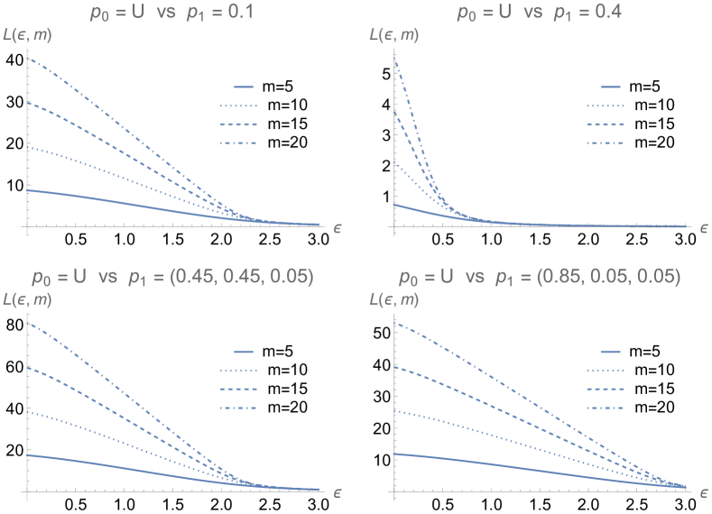
Theorem 4 shows that, as increases, becomes close to , and, for a fixed , the parameters and interact with and in order to control such a closeness. Empirical analyses in Rinott et al. (2017) show that, for a fixed and , the power decreases as decreases and/or increases; such a behaviour agrees with intuition, as decreasing and/or increasing leads to increase the perturbation in the data. Theorem 4 provides a theoretical guarantee to the analyses in Rinott et al. (2017) by quantifying the contribution of the truncated Laplace EM, in terms of and , to the power of the “true” LR test. According to (12), the truncated Laplace EM gives its most significant contribution in the term of order , whereas in the limit its contribution vanishes. That is,
determines the loss in the power of the “true” LR test. Since increases as decreases and/or increases, then the power of the “true” LR test decreases under such a behavior of and . See Figure 1 for an illustration of such a behaviour in the problem of testing a Uniform (U) , with and , versus some alternatives for ’s. Along the same lines of the proof of Theorem 4, it is easy to show that an analogous result holds true for the truncated Gaussian EM, with being replaced by such that the ’s are random variables i.i.d. according to (6). For fixed values of and , that is fixed levels of -DP, for the same tests considered in Figure 1, Table 1 shows that the truncated Laplace EM produces a smaller decrease in the power than the truncated Gaussian EM.
Remark 6.
Theorem 4 shows that the contribution of the truncated Laplace EM to the power of the “true” LR test vanishes in the limit , leading to (11). In particular, given a constant , a value of that solve
say , provides the correct scaling for the parameters and , with respect to the sample size , so that the contribution of the truncate Laplace EM to the power of the “true” LR test does no longer vanish in the large limit.
| L | G | L | G | L | G | L | G | L | G | |
|---|---|---|---|---|---|---|---|---|---|---|
| (0.025, 0.09) | 5 | 5 | 8.652 | 8.674 | 0.698 | 0.707 | 17.303 | 17.349 | 11.773 | 11.796 |
| (0.025, 0.04) | 10 | 10 | 18.927 | 18.972 | 2.037 | 2.069 | 37.854 | 37.944 | 25.228 | 25.274 |
| (0.05, 0.08) | 5 | 5 | 8.596 | 8.642 | 0.6789 | 0.697 | 17.191 | 17.284 | 11.715 | 11.762 |
| (0.05, 0.04) | 10 | 10 | 18.802 | 18.899 | 1.962 | 2.029 | 37.605 | 37.795 | 25.101 | 25.197 |
| (0.075, 0.08) | 5 | 5 | 8.538 | 8.610 | 0.660 | 0.687 | 17.076 | 17.219 | 11.656 | 11.729 |
| (0.075, 0.03) | 10 | 11 | 18.672 | 20.902 | 1.885 | 2.281 | 37.345 | 41.803 | 24.970 | 27.836 |
| (0.1, 0.07) | 5 | 6 | 8.479 | 10.573 | 0.641 | 0.903 | 16.958 | 21.147 | 11.595 | 14.327 |
| (0.1, 0.03) | 10 | 12 | 18.536 | 22.893 | 1.807 | 2.525 | 37.073 | 45.786 | 24.833 | 30.462 |
| (0.125, 0.07) | 5 | 6 | 8.419 | 10.531 | 0.622 | 0.888 | 16.837 | 21.063 | 11.533 | 14.283 |
| (0.125, 0.02) | 10 | 12 | 18.396 | 22.795 | 1.727 | 2.470 | 36.792 | 45.591 | 24.690 | 30.362 |
| (0.150, 0.06) | 5 | 6 | 8.357 | 10.489 | 0.603 | 0.874 | 16.713 | 20.978 | 11.469 | 14.240 |
| (0.150, 0.02) | 10 | 12 | 18.250 | 22.696 | 1.646 | 2.414 | 36.499 | 45.391 | 24.542 | 30.261 |
| (0.175, 0.06) | 5 | 6 | 8.293 | 10.446 | 0.584 | 0.859 | 16.587 | 20.892 | 11.404 | 14.195 |
| (0.175, 0.02) | 10 | 12 | 18.098 | 22.595 | 1.565 | 2.358 | 36.197 | 45.189 | 24.389 | 30.158 |
| (0.2, 0.05) | 5 | 6 | 8.228 | 10.403 | 0.565 | 0.845 | 16.457 | 20.801 | 11.337 | 14.150 |
| (0.2, 0.02) | 10 | 13 | 17.942 | 24.536 | 1.483 | 2.566 | 35.884 | 49.072 | 24.231 | 32.734 |
Theorem 4 allows us to define the loss of power of the “true” LR test, which admits a natural formulation as the additional sample size that is required in the “true” LR test in order to recover the power of the Multinomial LR test. According to Theorem 4, for any fixed value of the power, there exist: i) an integer such that, for , the LR test in the absence of perturbation has eventually power not less than ; ii) an integer such that, for , the “true” LR test has eventually power not less than . That is, and provide lower bounds for the sample size required to obtain a power (at least equal to) . Accordingly, for any such that , we can make use of the large asymptotic expansions of and in Theorem 4 to quantify and and, above all, the gap between these lower bounds. In particular, from (12) we can write
with
where means that and are obtained after dropping the -term on the right-hand side of (12). Therefore, the gap between and takes on the interpretation of the (sample) cost of -DP under the “true” LR test. That is, the additional sample size required to recover the power of the Multinomial LR test.
We conclude with a brief discussion on the effect of the dimension on the power of the “true” LR test. Theorem 4 shows how the sample size interacts with the truncated Laplace EM. However, according to Theorem 4, also interacts with the truncated Laplace EM, still in terms of the parameters and , thus having a direct effect on the power of the “true” LR test. By maintaining the sample size large enough, we assume that increases moderately. Differently from the sample size , any increase of the dimension determines a corresponding change of and , as these probabilities are elements of . Therefore, instead of the sole , it is critical to consider a suitable function of , and , say , and then show how such a function interacts with the truncated Laplace EM. From (12), it is clear that the interaction between and the parameters and is determined by . The behaviour of such a term depends on the specific form of the moment generating function of the Laplace distribution (4), which turns out to be a convex, even function with a global minimum at . The larger the flatter the -shape of this function around its minimum. Since is the sum of logarithmic terms, it is critical to count the number of terms in the sum that are not of the form , for some small . That is, the number of “large-scale terms”:
By a suitable tuning of , the quantity gives the number of large-scale terms. The next proposition shows how interacts with the truncated Laplace EM, and its impact on the power of the “true” LR test.
Proposition 7.
Under the assumptions of Theorem 4, for a given , it holds that
-
i)
if then the contribution of to the power of the “true” LR test decreases at least proportionally to the quantity
-
ii)
if and then the contribution of to the power of the “true” LR decreases proportionally to
See Appendix B for the proof of Proposition 7. According to Proposition 7, the choice of the parameter determines a “large scale” and a “small scale” for the terms that are involved in the sum defined through . Under the large scale behaviour of , i.e. , Proposition 7 shows that there exists an interaction between and the parameters and , and that such an interaction is with respect to . Under the small scale behaviour of , i.e. , Proposition 7 shows that the exists an interaction between and the parameters and , and that such an interaction is with respect to . The small scale behaviour thus leads to an interaction directly in terms of the dimension , thus showing clearly the effect of on the power of the “true” LR test. In particular, under the small scale behaviour, the contribution of to the power of the “true” LR test decreases proportionally to . That is, the smaller and the smaller , i.e. the larger and/or the smaller , the smaller is the contribution of to the power of the “true” LR test.
4 A “naïve” LR test for goodness-of-fit under -DP
As in Section 3, we assume that is perturbed by means of the truncated Laplace EM, in such a way that the resulting perturbed list has the same sample size as the original list . Then, to avoid the release of negative values, we assume that is post-processed in such a way that the negative values of are replaced by zeros (Rinott et al., 2017, Section 6). That is, we define , where for and . Note that the sample size of may be different from the sample size of . Assuming that is modeled as the “true” model described in Section 3, i.e. is the realization of the random variable and , it is natural to model as the realization of the random variable with for and . Therefore, differently from , the sample size of is random. Following the work of Rinott et al. (2017), we consider a “naïve” model for the perturbed list , that is a statistical model that does not takes into account the truncated Laplace EM. The “naïve” model assumes that is modeled as the distribution of the random variable such that the conditional distribution of given is a Multinomial distribution with parameter . Under the “naïve” model for , we make use of the LR test to assess goodness-of-fit in the form: , for a fixed , against . As in Section 3, without loss of generality, we assume that belongs to the interior of .
Remark 8.
A straightforward application of classical concentration inequalities for the Multinomial distribution entails that, for any fixed , the probability of the event can be bounded by an exponential term of the form , for a suitable choice of . This result shows that the additional randomness carried by the sample size does not contribute in any significant way to the Edgeworth expansions of the distribution of the “naïve” LR in Theorem 9 and Theorem 10 below, where only terms of and -type are relevant. We refer to Remark 17 for further details.
Under the “naïve” model for the post-processed list , the likelihood function is
| (14) |
Now, for the sake of simplicity, we start developing an asymptotic analysis under the assumption that . That is, has a Binomial distribution with parameter , is independent of and distributed according to (4), and . Under the “naïve” model with , we make use of the LR test to assess goodness-of-fit in the form: , for a fixed , against . Recall that the LR under the “true” model is given by (7) with . We denote by the maximum likelihood estimator of under the “naïve” model for , that is the estimator obtained through the maximization of the likelihood function (14) with . Then, we define
which is referred to as the “naïve” LR, and we denote by the distribution of computed with respect to distributed as a Binomial distribution with parameter . The next theorem establishes an Edgeworth expansion, with respect to , for the distribution of . To emphasize the comparison with respect to the “true” model, we also include the Edgeworth expansion of the distribution of , which follows from Theorem 3 with . We denote by the the cumulative distribution function of a chi-squared distribution with degree of freedom.
Theorem 9.
Let be the cumulative distribution function of , and let be the cumulative distribution function of . For any and any
| (15) |
with
and
| (16) |
with
where: the functions and are independent of and of the distribution of , that is independent of and ; the function is independent of and such that ; the functions and are independent of .
See Appendix A for the proof of Theorem 9. The functions , and in Theorem 9, as well as the functions and , can be made explicit by gathering some equations in the proof of the theorem. To assess goodness-of-fit by means of and , we fix a (reference) level of significance and find and such that and , respectively. Then, we define the rejection regions and . Some empirical analyses in Rinott et al. (2017) show that the “true” LR test has statistical significance at level , with a power that varies with and , whereas the “naïve” LR test has no statistical significance at the same level . Theorem 9 provides a theoretical guarantee to such empirical analyses, showing that the term determines the loss in the statistical significance of the “naïve” LR test. For a fixed , the variance of the truncated Laplace EM is critical to control the closeness between and : the larger the less close to , and hence the larger the less the statistical significance of the “naïve” LR test. Note that increases as decreases and/or increases. Then, the loss in the statistical significance of the “naïve” LR test is driven by and , through , in combination with . Along the same lines of the proof of Theorem 3, it is easy to show that an analogous result holds true for any convolutional-type EM. In particular, for the truncated Gaussian EM, Theorem 3 holds true with the variance of replaced by the variance of with distribution (6). For some fixed values of and , that is fixed levels of -DP, Table 2 shows that , and hence the truncated Laplace EM produces a smaller loss of statistical significance in the “naïve” LR test than the truncated Gaussian EM.
| L | G | |||
|---|---|---|---|---|
| (0.025, 0.09) | 5 | 5 | 9.660 | 9.824 |
| (0.025, 0.04) | 10 | 10 | 34.288 | 35.411 |
| (0.05, 0.08) | 5 | 5 | 9.650 | 9.324 |
| (0.05, 0.04) | 10 | 10 | 31.965 | 34.187 |
| (0.075, 0.08) | 5 | 5 | 8.991 | 9.478 |
| (0.075, 0.03) | 10 | 11 | 29.711 | 39.189 |
| (0.1, 0.07) | 5 | 6 | 8.662 | 12.850 |
| (0.1, 0.03) | 10 | 12 | 27.541 | 43.925 |
| (0.125, 0.07) | 5 | 6 | 8.337 | 12.574 |
| (0.125, 0.02) | 10 | 12 | 25.465 | 42.084 |
| (0.150, 0.06) | 5 | 6 | 8.019 | 12.303 |
| (0.150, 0.02) | 10 | 12 | 23.493 | 40.317 |
| (0.175, 0.06) | 5 | 6 | 7.706 | 12.037 |
| (0.175, 0.02) | 10 | 12 | 21.631 | 38.624 |
| (0.2, 0.05) | 5 | 6 | 7.399 | 11.776 |
| (0.2, 0.02) | 10 | 13 | 19.884 | 42.001 |
We conclude by extending Theorem 9 to an arbitrary dimension . Note that it is sufficient to present such an extension under the “naïve” mode, as the extension under the “true” model is precisely Theorem 3. Recall that is distributed as a Multinomial distribution with parameter , is independent of and with the ’s being random variables i.i.d. according to (4), and with for and . Under the “naïve” model, we make use of the LR test to assess goodness-of-fit in the form: , for a fixed , against . The LR under the “true” model is given by (7). We denote by be the maximum likelihood estimator of under the “naïve” model for , that is the estimator obtained through the maximization of the likelihood function (14). Then, we define the LR
which is referred to as the “naïve” LR, and we denote by the distribution of computed with respect to distributed as a Multinomial distribution with parameter . As , the theorem establishes an Edgeworth expansion for the distribution of “naïve” LR, . With respect to , there is a new element to take into account, that is the covariance matrix whose entry is for and by for .
Theorem 10.
Let denote the Fisher information matrix of the Multinomial model with parameter , and let be the cumulative distribution function of . For any and any
| (17) | ||||
with
where the functions and are independent of and of the distribution of , i.e. independent of and , and the function is independent of .
See Appendix B for the proof of Theorem 10. Theorem 10 leads to the same conclusions as Theorem 9, showing the critical role of the Laplace perturbation mechanism. In general, Theorem 9 and Theorem 10 highlight the importance of taking the perturbation into account in privacy-protecting LR tests for goodness-of-fit, and therefore the importance of negative values in the released list . Official statistical agencies are typically reluctant to disseminate perturbed tables with negative frequencies, and hence a common policy to preserve -DP consists in reporting negative values as zeros. However, as a matter of fact, releasing tables that have an appearance similar to that of original tables may lead to ignoring the perturbation and to analyzing data as they were not perturbed, i.e. under the “naïve” model (Rinott et al., 2017). Our analysis shows the importance of taking the perturbation into account, i.e. the importance of the “true” model versus the “naïve”, showing a loss in the statistical significance of the test when perturbed data are treated as they were not perturbed. Such a loss provides an evidence of the importance of taking the perturbation into account in the statistical model, thus endorsing the release of negative values if -DP is adopted.
5 Discussion
Under the framework of -DP for frequency table, we developed a rigorous analysis of the large sample behaviour of the “true” LR test. Our main contributions are with respect to the power analysis of the “true” LR test, and they built upon a Bahadur-Rao large deviation expansion for the power of the “true” LR test. By relying on a novel (sharp) large deviation principle or sum of i.i.d. random vectors, such an expansion brought out the critical quantity , which determines a loss in the power of the “true” LR test. This result has then been applied to characterize the impact of the sample size and the dimension of the table, in connection with the parameters , on the loss of the power of the private LR test. In particular, we determined the (sample) cost of -DP under the “true” LR test, namely the additional sample size required to recover the power of the Multinomial LR test in the absence of perturbation. As a complement to our power analysis of the “true” LR test, we investigated the well-known problem of releasing negative values in frequency tables under the -DP. By comparing the Edgworth expansions for the distribution of the “true” LR test and the “naïve” LR test, we showed the importance of taking the perturbation into account in private LR tests for goodness-of-fit, thus providing the first rigorous evidence to endorse the release of negative values when -DP is adopted. Our work provides the first rigorous treatment of privacy-protecting LR tests for goodness-of-fit in frequency tables and, in particular, it is the first work to make use of the power of the test to quantify the trade-off between confidentiality and utility. This is achieved through a non-standard large deviation analysis of the LR test, which is known to be challenging in a setting such as ours, where the statistical model is multidimensional, discrete, and not belonging to the exponential family.
Our power analysis of the “true” LR test can be easily extended to any truncated convolutional-type EM. As an example, we considered the truncated Gaussian EM, comparing it with the truncated Laplace EM. A numerical comparison showed how the truncated Laplace EM produces a smaller decrease in the power of the “true” LR test than the truncated Gaussian EM. Such a finding leads to the natural problem of identifying the optimal truncated convolutional-type EM, that is the truncated convolutional-type EM that leads to the smallest decrease in the power of the “true” LR test. In particular, is the truncated Laplace EM the optimal convolutional-type EM? This is an interesting open problem, whose rigorous solution requires an extension of Theorem 4 to deal with truncated EMs such that for a general function . Based on the proof of Theorem 4, we conjecture that the resulting Bahadur-Rao large deviation expansion is still in the form (12), with a critical term at the order that depends on . Given that, one has to deal with a challenging optimization problem with respect to , that is finding that leads to the smallest decrease in the power of the “true” LR test. Along similar lines, one may consider the more general problem of identifying the optimal truncated EM, thus removing the assumption that . However, for a general EM, it is difficult to conjecture the corresponding generalization of Theorem 4. Still related to Theorem 4, an interesting open problem is to consider a scaling of the parameter with respect to the sample size , say , and then identify the right scaling for which the contribution of the truncated Laplace EM to the power of the “true” LR test does no longer vanish in the large limit.
Among other directions for future research, the study of optimal properties of the “true” LR is of special interest. In particular, for a fixed (reference) level of significance , let and denote the powers of an arbitrary test statistic and of the LR test, respectively, for testing testing against , for fixed . It is known from Bahadur (1960) that
| (18) |
and
That is, the LR test attains the lower bound (18). This is referred to as Bahadur efficiency of the LR test, and it provides a well-known optimal property of the LR test (Bahadur, 1960, 1967). An open problem emerging from our work is to establish a “private” version of the lower bound (18), and investigate the Bahadur efficiency of the “true” LR with respect to such a lower bound. Establishing such a property of optimality for the “true” LR test would provide a framework to compare goodness-of-fit tests under -DP.
Appendix A Proofs for
In this section we will prove Theorems 9 and 4 in the case that our data set is a table with two cells, i.e. when . Recall that, in this case, the statement of Theorem 3 is already included in that of Theorem 9. Thus, the observable variable reduces to the counting contained in the first cell. At the beginning, some preparatory steps are needed to analyze the likelihood, the MLE and the LR relative to the null hypothesis , under the true model (5).
A.1 Preparatory steps
First of all, let us state a proposition that fixes the exact expression of the likelihood under the true model (5).
Lemma 11.
Let and be fixed to define the Laplace distribution (4). Then, if and , we have
| (19) |
Moreover, under the same assumption, for any we can write
| (20) |
with
| (21) | ||||
| (22) | ||||
| (23) |
Proof.
Start from
| (24) |
where the random variables and , defined on the probability space , are independent, and has the Laplace distribution (4). By definition , so that, under the assumption of the Lemma, the independence of and entails
proving (19). Finally, the decomposition (20) ensues from straightforward algebraic manipulations. ∎
The next step aims at providing a large asymptotic expansion of the true likelihood. This expansion can be obtained by considering the observable quantity as itself dependent by , according to the following
Lemma 12.
Let be a fixed number. Under the assumption that with , there exists such that
| (25) | ||||
holds for any and , where
for some constant . Therefore, under the same assumption, there holds
| (26) | ||||
for any , where
with .
Proof.
We start by dealing with (25). First, we find in such a way that the assumptions of Lemma 11 are fulfilled for any . Now, if , then and the thesis follows trivially. Also, if , then and the validity of the thesis can be checked by direct computation. Then, if , we use (23) to get
where denotes the Stirling number of first kind. Whence,
At this stage, recalling that and , and exploiting the binomial formula, we have
for suitable expressions of (possibly different from line to line) satisfying, in any case, the relation
To proceed further, we exploit that as , to obtain
The thesis now follows by multiplying the last expression by that of , neglecting all the terms which are comparable with . Thus, (25) is proved also for all .
For the argument can be reduced to the previous case. In fact, since , we can put , and to obtain
This completes the proof of (25) since and , , and .
We can now provide a large asymptotic expansion for the MLE relative to the true likelihood , contained in the following
Lemma 13.
Under the same assumption of Lemma 12, there holds
| (27) |
Proof.
First, we get a large expansion for the -likelihood, as follows
where
for some constant . Then, to find the maximum point of the likelihood, we study the equation , which reads
The solution of such an equation can be obtained by inserting the expression in the place of , and then expanding both members. For the left-hand side we get
where . On the other hand, a Taylor expansion around yields for the right-hand side
Here, it is important to notice that we have disregarded all the terms of -type, considering them of lower order with respect to the terms of -type. This is due to the law of iterated logarithm, by which , when . Thus, requiring identity between the above expansions yields
At this stage, to complete the proof it remains to evaluate the various terms . We start with the terms involving . First, we notice that
After putting and noticing that
we get
Now, when , we have
and, hence,
Then, we consider the terms containing . We start from the identities
and
Now, when , we have
Finally, we consider the terms containing . We start from the identities
and
Now, when , we have
At the end of all these computation, we are in a position to conclude that proving (27). ∎
The way is now paved to analyze the LR relative to the null hypothesis , by means of the following
Lemma 14.
Under the same assumption of Lemma 12 with , there hold
| (28) |
along with
| (29) | ||||
and
| (30) |
Therefore, putting , we get
| (31) |
with
| (32) | ||||
| (33) | ||||
| (34) |
for suitable terms and .
Remark 15.
Notice that the expression inside the brackets in (29) coincides with the Taylor polynomial of order 4 of the map where
denotes the Kullback-Leibler divergence relative to the Bernoulli model. In particular, we have that
coincides with the Fisher information of the Bernoulli model. Finally, it is worth noticing that, in the Bernoulli model, the Fisher information just coincides with the inverse of the variance.
Proof.
Since
holds by definition, identity (28) follows immediately from (20). Next, we derive (29) by combining (21) with (27). In fact, we have
where , according to (27). Therefore, using the Taylor expansion of the function , we can further specialize the last expression as
At this stage, careful algebraic computations based on the Newton binomial formula lead to (29). Incidentally, it is interesting to notice that the terms and , depending on the perturbation, do not appear in the expansion (29).
The last preparatory result provides an equivalent reformulation of the event
| (35) |
for some , to be determined after assessing the level of the test.
Lemma 16.
Proof.
Since and eventually, we first notice that, always eventually, the graphic of the function
goes to as , decreases for , increases for , and has a unique absolute minimum at . Thus, for any (to be determined later on), the equation admits two real solutions, that we just denote as and . To evaluate them, we put
After inserting these expression into the function , we set equal to zero the coefficients of and , obtaining
Finally, to prove (37)-(38), it is enough to use (32)-(33)-(34) of Lemma 24, showing that
and
which concludes the proof. ∎
A.2 Proof of Theorem 9
We start again from (24) where the random variables and , defined on the probability space , are independent, and has the Laplace distribution (4). Thus, under the validity of , we define the event as
| (39) |
for some . By a standard large deviation argument (see, e.g., Theorem 1 of Okamoto (1959)), there holds
which implies that the probability can be made arbitrarily small after a suitable choice of . See also Proposition 2.1 of Dolera and Regazzini (2019) for more refined bounds. In particular, it can be chosen so that
| (40) |
In this way, for , we can write
with
The advantage of such a preliminary step is that, on , the assumptions of all the Lemmata stated in the previous subsection are fulfilled and, by resorting to (36), we can write
where
| (41) |
with
Remark 17.
This very same argument, based on straightforward application of concentration inequalities for the Binomial distribution, makes clear that the additional randomness that emerges in the “naïve” model, due to the presence of the random sample size , is irrelevant in our asymptotic analysis. Indeed, after fixing , we get that the probability that (that is, the first cell contains a negative value) is bounded by a term of the form for some . Since terms of this form are irrelevant in the Edgeworth expansion (16), we can work from the beginning under the assumption that (that is, the first cell does not contain a negative value) which entails, in particular, that . An analogous consideration holds in larger dimensions, that is when , if is fixed in the interior of .
Therefore, in view of (40), we can conclude that
| (42) |
where denotes the distribution function of . Moreover, the same analysis developed in the previous section shows that
| (43) |
with
| (44) | ||||
| (45) |
Therefore, it is evident from the previous identities that the proof of Theorem 9 can be carried out after providing an explicit expansion of Berry-Esseen type of , which is contained in the following
Proposition 18.
Let denote the cumulative distribution function of the standard Normal distribution, and let, for any ,
In addition, for any , let denote the function
where means that the sum ranges over all the -uples such that , with , denotes the Chebyshev-Hermite polynomial, i.e.
and stands for the cumulant of the Bernoulli distribution of parameter . Then, for any , there holds
with the remainder term satisfying an inequality like
for some suitable constant independent of .
Proof.
After denoting by the distribution function of , invoke well-known results (see, e.g., Theorem 6 in Chapter VI of Petrov Petrov (1975), or Dolera and Favaro (2020)) to write (in the same notation adopted by Petrov)
where and
for some positive constant . Now, in view of the definition of , its distribution function is given by
To obtain an expansion for , notice that, for , there holds
thanks to the periodic character of . Hence, the effect of putting is mainly observed in the terms , , and : by resorting to the Taylor expansion, for any , write
where the remainder term satisfies
for some positive constant . Thus, exploiting the symmetry of the Laplace distribution, obtain
where the remainder term satisfies
for some suitable constant independent of . Finally, gathering the previous identities, conclude that
Incorporating all the terms of type in the remainder yields the thesis to be proved. ∎
The way is now paved to complete the proof of Theorem 9. Indeed, (15) follows by combining the thesis of Proposition 18 with (42) and (37)-(38). To see this, we start from the analysis of the quantity
which represents the “regular” part of the expression of (42). Taking account of (37)-(38), a straightforward Taylor expansion shows that the above quantity is equal to
Exploiting that , we show that the terms containing cancel out. Moreover, and hold for any . These considerations lead to the following equivalent reformulation of the above term
This is the main part of the proof. Then, we deal with the “irregular” part of the expression of (42). The argument is essentially the same as above, even if we have now to take care of the expressions
for , which are not smooth functions. Anyway, for any fixed such that the quantity is not a singularity of , we can actually apply the Taylor formula, since the are smooth away from their singularities. With this trick we show that the “irregular” part of (42) provides the quantity , where
The only term which is not caught by this technique is
which corresponds to the terms in (15). Therefore, we can finally set
Then, we pass to the analysis of the quantity
which represents the “regular” part of the expression of (43). Again expanding by the Taylor formula, we get the equivalent expression
Since and the “irregular” part contained in is the same as above, we conclude the validity of (16), proving the theorem.
A.3 Proof of Theorem 4 for
We start again from (24) where the random variables and , defined on the probability space , are independent, and has the Laplace distribution (4). After fixing such that , according to Theorem 9, we have that
First, for , we define the event as
| (46) |
Then, recalling that
is a fixed quantity, we resort once again on a large deviation argument to choose sufficiently small so that
| (47) |
holds for some . In this way, we can write
with
Then, for , we define another event as
| (48) |
and we write
The advantage of such a preliminary step is that, on , the assumptions of all the Lemmata stated in the previous subsection are fulfilled and, by resorting to (36), we can write
where is the same random variable as in (41). Moreover, if , as we will choose, we have eventually that
It remains to show that, for a suitable choice of , we have
| (49) |
eventually, yielding that
| (50) |
The proof of (49), along with the proper choice of , is contained in the following
Lemma 19.
If and , with
then, eventually, there holds
Proof.
At this stage, we come back to (50) by writing
with
and . Thus, the event considered in (50) can be rewritten in terms of the random variable as follows
We now introduce the distribution function of , and we notice that (50) becomes
| (51) |
At this stage, we are in a position to apply Theorem 10 in Chapter VIII of Petrov (1975). Supposing, for instance that , we have that
| (52) |
where stands for the so-called Cramér-Petrov series relative to the Bernoulli distribution of parameter . Thus, putting
we proceed by resorting to the well-known Mills approximation to write
Therefore, (52) can be simplified as follows
At this stage, to complete the proof, we need a technical result that characterizes the expression in an exponential model parametrized by the mean.
Lemma 20.
Let be a measurable space, endowed with a -finite reference measure . Let be a measurable map such that the set
is open and convex. Putting , and , we have that is open and is a smooth diffeomorphism between and . Moreover, the family of -densities given by
defines a regular exponential family parametrized by the mean. Moreover, we have
where . For , putting
we have that
| (53) |
for every , where denotes the Cramér-Petrov series relative to the distribution of , with . Finally, for a generic dimension , putting , we have that
| (54) |
if is defined as the solution of the equation .
Proof.
For the main part of the lemma, we just quote any good reference on exponential families, such as Barndorff-Nielsen (1978). Here, we only prove (53). Putting , we have by definition that
where and is the solution of the equation . Thus, the last equation can be rewritten as . Whence,
completing the proof of (53). The same computation in generic dimension yields (54). ∎
At this stage, noticing that the family of Bernoulli distributions is a member of the regular exponential family parametrized by the mean, we can apply (53) with and to conclude that
Thus, if , we have
and we conclude that
As a last step of the proof, we expand the above expression containing by the Taylor formula, obtaining
In conclusion, we get
which entails the thesis of the theorem.
Appendix B Proofs for
In this section we will prove Theorems 3, 10 and 4 in the case that our data set is a table with more than two cells, i.e. when . Thus, the observable variable reduces to the countings contained in the first cells. Here, we state some preparatory results as in Appendix A.
B.1 Preparatory steps
First of all, let us state a proposition that fixes the exact expression of the likelihood under the true model (5).
Lemma 21.
Let and be fixed to define the Laplace distribution (4). Then, if and for , we have
| (55) | ||||
Moreover, under the same assumption, for any in the interior of we can write
| (56) |
with
| (57) | ||||
| (58) | ||||
| (59) |
Proof.
Start from
| (60) |
where the random variables and , defined on the probability space , are independent, and is a random vector with independent components with each having the Laplace distribution (4). By definition , so that, under the assumption of the Lemma, the independence of and entails
proving (55). Finally, the decomposition (56) ensues from straightforward algebraic manipulations. ∎
The next result is a multidimensional analogue of Lemma 12, that can be obtained by considering the observable quantity as itself dependent by . This task proves very cumbersome for a general dimension so that, in the remaining part of the subsection, we will confine ourselves to dealing with the case .
Lemma 22.
Let be a fixed vector. Under the assumption that with , there exists such that
| (61) | ||||
holds for any and , where
for some constant . Therefore, under the same assumption, there holds
| (62) | ||||
for any , where
with and
Proof.
We start by dealing with (61). First, we find in such a way that the assumptions of Lemma 11 are fulfilled for any . Then, as in the proof of Lemma 12, the thesis can be checked by direct computation if either or . Now, if , we use (59) to get
where again denotes the Stirling number of first kind. Whence,
At this stage, recalling that and , and exploiting the binomial formula, we have
for suitable expressions of (possibly different from line to line) which are, in any case, bounded by an expression like . To proceed further, we exploit that as , to obtain
The thesis now follows by multiplying the last expression by that of , neglecting all the terms which are comparable with . Thus, (25) is proved also for all . If either or the argument can be reduced to the previous case, as in the proof of Lemma 12. This completes the proof of (61).
The way is now paved to state a result on the expansion of the MLE which is analogous to Lemma 13
Lemma 23.
Proof.
We provide only a sketch of the proof, since the ensuing computations are too heavy to be fully reproduced. In any case, we start by providing a large expansion for the -likelihood, as follows
where, upon denoting by the outer product between vectors,
for some constant . Then, to find the maximum point of the likelihood, we study the equation , which reads
The solution of such an equation can be obtained by inserting the expression in the place of , , and then expanding both members. By carefully carrying out all of these computations, we are in a position to conclude that , and , thus completing the proof. ∎
The last preparatory result is the multidimensional analogous of Lemma 24.
Lemma 24.
Under the same assumption of Lemma 22 with , there hold
| (64) |
Moreover, we have
| (65) |
where denotes the Fisher information matrix of the Multinomial model which, for , reads
and
| (66) | ||||
Therefore, putting , we get
| (67) | ||||
| (68) |
Proof.
Next, we derive (65) by combining (57) with (63). In any case, a quicker argument can be based on Remark 15, according to which the right-hand side of (65) coincides with the Taylor expansion of the map . Thus, the result to be proved boils down to the application of the well-known relationship between the Kullback-Leibler divergence and the Fisher information matrix in a regular parametric model.
B.2 Proof of Theorems 3 and 10
We start again from (60) where the random variables and , defined on the probability space , are independent, and is a random vector with independent components with each having the Laplace distribution (4). Thus, under the validity of , we define the event as
| (69) |
for some . After recalling that each component of is a Binomial random variable, we can reduce the problem to the analogous one already treated in Section A.2, and we can find so that
| (70) |
In this way, for , we can write
with
The advantage of such a preliminary step is that, on , the assumptions of all the Lemmata stated in the previous subsection are fulfilled and, by resorting to (67), we can write
where
| (71) |
with
and is the covariance matrix of .
As in the preliminary part of this second Appendix, we confine ourselves to dealing with the case of . The following proposition represents the multidimensional analogous of the Berry-Esseen expansion already given in Proposition 18.
Proposition 25.
Let denote the density of the 2-dimensional Normal distribution with mean equal to and covariance matrix equal to , and let stand for the associated distribution function. In addition, for any multi-index , denote by the -cumulant of the random vector , and put to set
where is a shorthand to indicate that the summation is extended to all the -uples such that . Afterwords, define
and . Finally, set
and
where and are the same as in Proposition 18. Then, for any , there holds
| (72) |
with the remainder term satisfying an inequality like
for some suitable constant independent of .
Proof.
We start by putting
By independence, we have
At this stage, we exploit the well-known asymptotic expansions of displayed, e.g., in Section 23 of Bhattacharya and Rao (2010). We put in Theorem 23.1 to obtain
where is a remainder term satisfying an inequality like
for some suitable constant independent of . The key remark is about the modification of the terms of the type after the substitution . Indeed, we have
because of the periodicity of the ’s. Therefore, the substitution affects the functions and only in the terms involving , , , and their derivatives. Since these functions are smooth, we can apply the Taylor formula to get
for any multi-index , and analogous expansions for . Now, the assumption on the distribution of entails that as soon as either or is odd. Whence,
for any multi-index , and analogous expansions for the term
This completes the proof. ∎
At this stage, like in the previous proof of Theorem 9, the thesis of Theorems 3 and 10 follow from the combination of the Berry-Esseen expansion (72) with identity (67). Indeed, (72) shows that the probability distribution of has both an absolutely continuous part as well as a singular part. As before, the core of the proof hinges on the study of the absolutely continuous part, which is significantly affected by the Laplace perturbation because of the term . Thus, the sum
yields the following density (with respect to the 2-dimensional Lebesgue measure)
where denotes the density of the 2-dimensional Normal distribution with mean and covariance matrix , is the covariance matrix of the random vector , stands for the Laplacian operator, and is the trace operator. At this stage, it is enough to notice that the principal term of the expression of is given by the following integral
To handle the last integral, we start by noticing that
Thus, combining the last identities, we get
In view of the identity , we can use the Taylor formula to write
Now, it is crucial to observe that, for the Multinomial model, it holds . Whence,
where stands for the density of the standard Normal distribution. In conclusion, we have
Then, invoking the Taylor formula for the determinant operator, we get
which entails
This argument proves rigorously the presence pf the terms in (9). Now, we take cognizance that the expressions of , , and in (9) ensue from the various terms in (72), according to the above line of reasoning. In particular, ensues from the term that figures in the expression of , while corresponds to the manipulation of the quantity which also figures in the expression of . Furthermore, ensues from the expression of . However, what is crucial is just to remark once again is that the additional term
that appears in (72), which depends significantly on the Laplace perturbation, is no more present in (9).
It remains to justify the expression of , which follows from the combination of the Berry-Esseen expansion (72) with identity (68). Indeed, the core of the argument consists in the study of the integral , which equal to
Then, we can pass to polar coordinates and notice that
with . Finally, we have
which completes the proof of (17).
B.3 Proof of (13)
Upon putting , we prove that
| (73) |
is valid as , where is the dimension of the random vectors . The proof is a small variation of a classical argument developed, e.g., in Chapter VIII of Petrov (1975), in von Bahr (1967), or in Aleshkyavichene (1983).
Letting the distribution of be denoted by , we introduce the new probability measure for some and, then, a sequence of i.i.d. random vectors with distribution . We also put and . Hence, setting , we find that
yielding in turn, after some manipulations, that
| (74) |
with
At this stage, exploiting the assumption of the existence of for which , we choose so that (74) becomes
Therefore, to prove (73), it is enough to show that
as . Indeed, upon denoting by the standard Normal distribution on , we can write
| (75) |
For the former term on the right-hand side of (75), we have
where, in the last identity, is a constant depending solely on . For completeness, the validity of such an identity follows from a direct application of the multidimensional Laplace method displayed, e.g., in Theorem 46 of Breitung (1994). It remains to show that the absolute value of the latter term on the right-hand side of (75) is even less significant, as it can be bounded by an expression like
| (76) |
with some constant depending solely on . This task can be carried out by resorting to the Plancherel identity, i.e.
where
Therefore, we can write
| (77) |
with
the former of the above identities following once again from the multidimensional Laplace method. Thus, for the first integral on the right-hand side of (77), an application of inequalities (8.22)-(8.23) of Bhattacharya and Rao (2010)—which constitute a multidimensional generalization of the well-known Berry-Esseen inequalities—shows that
holds for some constant depending solely on . Then, the second integral on the right-hand side of (77) is asymptotically equivalent to the integral
as . Lastly, the last integral on the right-hand side of (77) has different behaviors according on whether the distribution is lattice or not. If , then the integral at issue is exponentially small like the second integral on the right-hand side of (77) described above. Otherwise, in the lattice case (which is of interest here), we deduce the expansion (76) by using the expression of (explicitly available in the lattice case) and by resorting once again to the multidimensional Laplace method.
B.4 Proof of Theorem 4 for
We start again from (60) where the random variables and , defined on the probability space , are independent, and is a random vector with independent components with each having the Laplace distribution (4). After fixing such that , according to Theorem 3, we have that
First, for , we define the event as
| (78) |
Then, recalling that
is a fixed quantity, we resort once again on a large deviation argument to choose sufficiently small so that
| (79) |
holds for some . In this way, we can write
with
Then, for , we define another event as
| (80) |
and we write
The advantage of such a preliminary step is that, on , the assumptions of all the preparatory Lemmata contained in Appendix B are fulfilled and, by resorting to (67), we can write
where is the same random variable as in (83). Moreover, if , as we will choose, we have eventually that
It remains to show that, for a suitable choice of , we have
| (81) |
eventually, yielding that
| (82) | ||||
The proof of (81), along with the proper choice of , follows as an application of Lemma 19 component-wise.
Afterwords, we come back to (82) by writing
| (83) |
where ,
and denotes the covariance matrix of . Exploiting the independence between and , upon putting
we get
| (84) | ||||
Now, we apply (13) to a sequence of i.i.d. random vectors taking values in , in such a way that
| (85) |
Moreover, we can put and
Actually, the equation that defines could be specified in a more precise way, as we have done for . In fact, exploiting the analogy with the case , we could write the big- term as
for suitable tensors and of third and fourth order respectively, both satisfying analogous expansions similar to (33)–(34). However, despite the cumbersome computation that would have needed to derive such quantities, we have already learnt from the case that they do not play any active role in the final result encapsulated in (12). More precisely, we know that the 0-order terms in and would ensue from the Taylor expansion of the map , while the successive terms in their expansion—which explicitly depend on the Laplace perturbation—do not affect the expressions of and in (12). Indeed, after defining the vector by means of the identity , where , we are now able to derive also the term in (12). After noticing that the above distribution (85) is a member of the regular exponential family parametrized by the mean, we can resort to Lemma 20 and apply (54) with and , where , to conclude that
Therefore, combining this last equation with (13) and (84) we get
which entails the thesis of the theorem, upon noticing that the quantity contains more explicit terms that depend on the Laplace perturbation only at the level . This ends the proof.
B.5 Proof of Proposition 7
First, we notice that
| (86) |
and . In particular, if , the main contribution comes from the sum over , so that , where denotes a small remainder term. In particular, if , then
holds. If , then the relevant part of the sum on the right-hand side of (86) is given by the sum of summands, each of which greater than . Finally, if and , we use the Taylor expansion of the logarithm to obtain that
holds as . Thus, if all the components of are less than , we get that the main contribution in the sum on the right-hand side of (86) is given by . This completes the proof.
Acknowledgement
The authors are very grateful to an Associate Editor and three Referees for their comments and suggestions that improved remarkably the paper. Emanuele Dolera and Stefano Favaro are grateful to Professor Yosef Rinott for suggesting the problem and for the numerous stimulating conversations and valuable suggestions. Emanuele Dolera and Stefano Favaro received funding from the European Research Council (ERC) under the European Union’s Horizon 2020 research and innovation programme under grant agreement No 817257. Emanuele Dolera and Stefano Favaro gratefully acknowledge the financial support from the Italian Ministry of Education, University and Research (MIUR), “Dipartimenti di Eccellenza” grant agreement 2018-2022.
References
- Acharya et al. (2018) Acharya, J., Sun, Z. and Zhang, H. (2018). Differentially private testing of identity and closeness of discrete distributions. In Neural Information Processing Systems.
- Aleshkyavichene (1983) Aleshkyavichene, A.K. (1983). Multidimensional integral limit theorems for large deviation probabilities. Theory of Probability and its Applications 28, 65–88.
- Aliakbarpour et al. (2018) Aliakbarpour, M., Diakonikolas, I. and Rubinfeld, R. (2018). Differentially private identity and equivalence testing of discrete distributions. In Proceedings of the International Conference on Machine Learning.
- Awan and Slavković (2018) Awan, J. and Slavković (2018). Differentially private uniformly most powerful tests for Binomial data. In Neural Information Processing Systems.
- Bahadur (1960) Bahadur, R.R. (1960). Stochastic comparison of tests. Annals of Mathematical Statistics 31, 276–295.
- Bahadur (1967) Bahadur, R.R. (1967). An optimal property of the likelihood-ratio statistic. Berkeley Symposium on Mathematical Statistics and Probability, 13–26.
- Barndorff-Nielsen (1978) Barndorff-Nielsen, O. (1978). Information and Exponential Families in Statistical Theory. Wiley.
- Bhattacharya and Rao (2010) Bhattacharya, R.N. and Rao, R.R. (2010). Normal approximation and asymptotic expansions. Wiley.
- Breitung (1994) Breitung, K.W. (1994). Asymptotic approximations for probability integrals. Springer.
- Cai et al. (2017) Cai, B., Daskalakis, C. and Kamath, G. (2017). Priv’IT: private and sample efficient identity testing. In Proceedings of the International Conference on Machine Learning.
- Canonne et al. (2019) Canonne, C.L., Kamath, G., McMillan, A., Smith, A. and Ullman, J. (2019). The structure of optimal private tests for simple hypotheses. In Proceedings of the ACM Symposium on the Theory of Computing.
- Canonne et al. (2020) Canonne, C.L., Kamath, G., McMillan, A., Ullman, J. and Zakynthinou, L. (2020). Private identity testing for high-dimensional distributions. In Neural Information Processing Systems.
- Cummings et al. (2018) Cummings, R., Krehbiel, S., Mei, Y., Tuo, R. and Zhang, W. (2018). Differentially private change-point detection. In Neural Information Processing Systems.
- Dolera and Favaro (2020) Dolera, E. and Favaro, S. (2020). Rates of convergence in de Finetti’s representation theorem, and Hausdorff moment problem. Bernoulli 26, 1296–1322.
- Dolera and Regazzini (2019) Dolera, E. and Regazzini, E. (2019). Uniform rates of the Glivenko–Cantelli convergence and their use in approximating Bayesian inferences. Bernoulli 25, 2982–3015.
- Dwork (2006) Dwork, C. (2006). Differential privacy. In Proceedings of the International Colloquium on Automata, Languages and Programming.
- Dwork et al. (2006) Dwork, C., McSherry, F., Nissim, K. and Smith, A. (2006). Calibrating noise to sensitivity in private data analysis. In Proceeding of the Theory of Cryptography Conference.
- Dwork and Roth (2013) Dwork, C. and Roth, A. (2013). The algorithmic foundations of differential privacy. Foundations and Trends in Theoretical Computer Science 9, 211–407.
- Efron (1967) Efron, B. (1967). The power of the likelihood-ratio test. Annals of Mathematical Statistics 38, 802–806.
- Efron and Truax (1968) Efron, B. and Truax, D. (1968). Large deviations theory in exponential families. Annals of Mathematical Statistics 39, 1402–1424.
- Ferguson (2002) Ferguson, T.S. (2002). A Course in large sample theory. Chapman and Hall/CRC.
- Fienberg et al. (2010) Fienberg, S.E., Rinaldo, A. and Yang, G. (2010).Differential privacy and the risk-utility trade-off for multi-dimensional contingency tables. In Proceedings of the International Conference on Privacy in Statistical Databases.
- Gaboardi et al. (2016) Gaboardi, M., Lim, H., Roger, R. and Vdhan, S. (2016). Differentially private chi-squared hypothesis testing: goodness-of-fit and independence testing. In Proceedings of the International Conference on Machine Learning.
- Hoeffding (1965) Hoeffding, W. (1965). Asymptotically optimal tests for multinomial distributions. Annals of Mathematical Statistics 36, 369–408.
- Hoeffding (1967) Hoeffding, W. (1967). On probabilities of large deviations. In Proceedings of the Fifth Berkeley Symposium on Mathematical Statistics and Probability.
- Kifer and Roger (2017) Kifer, D. and Rogers, R. (2017). A new class of private chi-square tests. In Proceedings of the International Conference on Artificial Intelligence and Statistics.
- Osipov (1982) Osipov, L.V. (1982). Large deviation probabilities of sums of independent random vectors for certain classes of sets. Mathematical Notes 31, 75–79.
- Okamoto (1959) Okamoto, M. (1959). Some inequalities relating to the partial sum of binomial probabilities. Annals of the Institute of Mathematical Statistics 10, 29–35.
- Petrov (1975) Petrov, V.V. (1975). Sum of independent random variables. Springer.
- Rao (1962) Rao, C.R. (1962). Efficient estimates and optimum inference procedures in large samples. Journal of the Royal Statistical Society Series B 24, 46–72.
- Rinott et al. (2017) Rinott, Y., O’Keefe, C.M., Shlomo, N. and Skinner, C. (2017). Confidentiality and differential privacy in the dissemination of frequency tables. Statistical Science 33, 358–385.
- Saulis (1983) Saulis, L. (1983). Large deviations for random vectors for certain classes of sets. Lithuanian Mathematical Journal 23, 308–317.
- Saulis and Statulevicius (1991) Saulis, L. and Statulevicius, V.A. (1991). Limit theorems for large deviations. Kluwer.
- Steinke and Ullman (2016) Steinke, T. and Ullman, J. (2016). Between pure and approximate differential privacy. Journal of Privacy and Confidentiality 7, 3–22.
- von Bahr (1967) von Bahr, B. (1967). Multi-dimensional integral limit theorems. Arkiv för Mathematik 7, 71–88.
- Wang et al. (2015) Wang, Y., Lee, J. and Kifer, D. (2015). Revisiting differentially private hypothesis tests for categorical data. Preprint arXiv:1511.03376.
- Wilks (1938) Wilks, S.S. (1938). The large-sample distribution of the likelihood-ratio for testing composite hypotheses. Annals of Mathematical Statistics 9, 60–62.