Formal derivation of quantum drift-diffusion equations
with spin-orbit interaction

Abstract.

Quantum drift-diffusion equations for a two-dimensional electron gas with spin-orbit interactions of Rashba type are formally derived from a collisional Wigner equation. The collisions are modeled by a Bhatnagar–Gross–Krook-type operator describing the relaxation of the electron gas to a local equilibrium that is given by the quantum maximum entropy principle. Because of non-commutativity properties of the operators, the standard diffusion scaling cannot be used in this context, and a hydrodynamic time scaling is required. A Chapman–Enskog procedure leads, up to first order in the relaxation time, to a system of nonlocal quantum drift-diffusion equations for the charge density and spin vector densities. Local equations including the Bohm potential are obtained in the semiclassical expansion up to second order in the scaled Planck constant. The main novelty of this work is that all spin components are considered, while previous models only consider special spin directions.

1. Introduction

Spintronics exploits the electron spin as a further degree of freedom in semiconductor materials. The objective of spintronics is to develop fast, high-capacity, and low-power information and communication devices. The design of spintronic structures is accelerated by numerical simulations that optimize the device properties. To achieve efficient but physically accurate simulations, macroscopic spin models, also including quantum features, are needed.

In the literature, usually simplified models are considered. A simple approach is to consider specific directions of the spin vector, for instance the spin-up and spin-down electron densities or, equivalently, the total density and the spin polarization [21]. A more complete picture is obtained by taking into account the complete spin vector and not only its projection on a given direction. Such models have four variables: the charge density and the densities of the three spin components [10, 18]. Quantum corrections have been included in the former approach in [3], leading to spinorial quantum drift-diffusion equations for the spin-up and spin-down densities, while the works [2, 18] are concerned with the derivation of full spin-vector models but without quantum corrections. Up to our knowledge, no drift-diffusion models with a full spin structure and quantum corrections have been derived in the literature so far. In this paper, we fill this gap by deriving spinorial quantum drift-diffusion equations for a two-dimensional electron gas from a collisional von Neumann equation.

1.1. Setting

We consider an electron gas confined in an asymmetric two-dimensional potential well. Then the electrons experience a spin-orbit interaction of Rashba type [4]. The Rashba effect is a momentum-based splitting of spin bands, which comes from the combined effect of spin-orbit interaction and an asymmetry of the potential. It manifests as an effective magnetic field orthogonal to the confinement direction and the electron motion; see Figure 1. The spin orientation can be indirectly controlled by the gate voltage, which deviates the electrons, thus changing the direction of the effective magnetic field. We refer to the review [22] for more details.

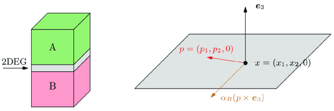
Figure 1. Left: A two-dimensional electron gas (2DEG) is confined between two different semiconductor materials A and B (for instance, InAlAs and InGaAs). Right: The electrons of the 2DEG experience an effective magnetic field $\alpha_{R}(p\times\bm{e}_{3})$ orthogonal to both the electron momentum $p$ and the confinement direction $\bm{e}_{3}$, where $\alpha_{R}>0$ and $\bm{e}_{3}=(0,0,1)^{T}$.

The motion of the confined electrons in the $(x_{1},x_{2})$-plane is governed by the (scaled) von Neumann equation for the density operator $\hat{\rho}(t)$,

(1) $${\mathrm{i}}\varepsilon\tau_{0}\partial_{t}\hat{\rho}=[\mathcal{H}_{\varepsilon},\hat{\rho}]:=\mathcal{H}_{\varepsilon}\hat{\rho}-\hat{\rho}\mathcal{H}_{\varepsilon},\quad t>0,$$

where the (scaled) Hamiltonian $\mathcal{H}_{\varepsilon}$ is the sum of the kinetic energy, potential energy, and spin-orbit interaction,

(2) $$\mathcal{H}_{\varepsilon}=\bigg{(}-\frac{\varepsilon^{2}}{2}\Delta+V(x)\bigg{)}\sigma_{0}-\varepsilon^{2}\alpha\begin{pmatrix}0&{\mathrm{i}}\partial_{x_{2}}-\partial_{x_{1}}\\ {\mathrm{i}}\partial_{x_{2}}+\partial_{x_{1}}&0\end{pmatrix}.$$

Here, the function $V(x)$ is the electric (gate) potential, $\sigma_{0}\in{\mathbb{C}}^{2\times 2}$ is the identity matrix, $\varepsilon>0$ is the scaled Planck constant, $\tau_{0}$ is a scaled time, and $\alpha>0$ is the scaled Rashba constant. We refer to Section 2.1 for details on the scaling.

Our derivation is based on the phase-space formulation using the Wigner transform $W:=\mathcal{W}(\hat{\rho})$, defined in (11) below. Then equation (1) transforms to the Wigner equation (see Lemma 6)

$$\tau_{0}\partial_{t}W+{\mathcal{T}}W=0,\quad t>0,$$

where ${\mathcal{T}}W=({\mathrm{i}}/\varepsilon)(H_{\varepsilon}\#W-W\#H_{\varepsilon})$ is the transport operator, $H_{\varepsilon}=\mathcal{W}(\mathcal{H}_{\varepsilon})$ is the Hamiltonian symbol, and $\#$ denotes the Moyal product defined in (14) below. To derive diffusion equations, we introduce a collision term of Bhatnagar–Gross–Krook (BGK) type:

(3) $$\tau_{0}\partial_{t}W+{\mathcal{T}}W=\frac{1}{\tau}({\mathcal{M}}(N)-W),\quad t>0,$$

where $\tau>0$ is the (scaled) relaxation time, ${\mathcal{M}}(N)=\mathcal{W}(\exp(-\mathcal{H}_{\varepsilon}+\tilde{A}))$ is the so-called quantum Maxwellian, which (formally) minimizes the quantum free energy under the constraint of a given density matrix $N=\langle W\rangle:=\int_{{\mathbb{R}}^{2}}Wdp$, and $\tilde{A}$ is the associated Lagrange multiplier; see Section 2.4 for details.

If the time scale $\tau_{0}$ is of the same order as the (scaled) relaxation time $\tau$, we obtain a diffusive scaling. The usual way to derive a macroscopic model is the Chapman–Enskog expansion. Let $W_{\tau}$ be a solution to (3) with $\tau_{0}=\tau$ and write $W_{\tau}=W_{0}+\tau G_{\tau}$ for two functions $W_{0}$ and $G_{\tau}$. The formal limit $\tau\to 0$ in (3) determines the first function, $W_{0}={\mathcal{M}}(N)$. The expansion $W_{\tau}=W_{0}+\tau G_{\tau}$ in fact defines $G_{\tau}$. Inserting this expansion into (3), dividing by $\tau$, and performing the formal limit $\tau\to 0$ leads to $G:=\lim_{\tau\to 0}G_{\tau}=-{\mathcal{T}}{\mathcal{M}}(N)$. The last step is to integrate (3) with respect to $p$,

$$\partial_{t}\langle W_{\tau}\rangle+\frac{1}{\tau}\langle{\mathcal{T}}{\mathcal{M}}(N)\rangle+\langle{\mathcal{T}}G_{\tau}\rangle=0,$$

and to pass to the limit $\tau\to 0$. In the classical situation, ${\mathcal{T}}{\mathcal{M}}(N)$ is an odd function in $p$ and therefore, its integral with respect to $p$ vanishes. Physically, this means that the equilibrium state ${\mathcal{M}}(N)$ has a vanishing diffusion current. The limit $\tau\to 0$ then leads to the macroscopic model $\partial_{t}N-\langle{\mathcal{T}}{\mathcal{T}}{\mathcal{M}}(N)\rangle=0$, where $\langle{\mathcal{T}}{\mathcal{T}}{\mathcal{M}}(N)\rangle$ is a drift-diffusion term. In the present case, however, it turns out that generally $\langle{\mathcal{T}}{\mathcal{M}}(N)\rangle\neq 0$ (see Lemma 8). This means that there is a residual current in the equilibrium state that is due to the spin-orbit interaction. We show in Lemma 8 that the condition $\langle{\mathcal{T}}{\mathcal{M}}(N)\rangle\neq 0$ can be characterized by the non-commutativity between the density matrix $N$ and the Lagrange multiplier $\tilde{A}$.

Therefore, we impose a hydrodynamic scaling, which is suitable for local equilibria with non-vanishing currents. We stress the fact that the BGK collisions do not conserve the current. The residual current ${\mathcal{T}}{\mathcal{M}}(N)$ is of quantum mechanical nature and in our case, it is of order $\varepsilon^{3}$ (see (30) and (48)). We suppose that $\tau_{0}$ is of order one, while $\tau\ll 1$. Then the expansion $W_{\tau}={\mathcal{M}}(N)+\tau G_{\tau}$ in (3) leads to $G_{\tau}=-\partial_{t}{\mathcal{M}}(N)-{\mathcal{T}}{\mathcal{M}}(N)+O(\tau)$. We integrate (3) with respect to $p$, divide the equation by $\tau$, and insert the expansion $W_{\tau}={\mathcal{M}}(N)-\tau(\partial_{t}{\mathcal{M}}(N)+{\mathcal{T}}{\mathcal{M}}(N))+O(\tau^{2})$:

$$\partial_{t}N=-\langle{\mathcal{T}}{\mathcal{M}}(N)\rangle=-\langle{\mathcal{T}}{\mathcal{M}}(N)\rangle+\tau\langle{\mathcal{T}}\partial_{t}{\mathcal{M}}(N)\rangle+\tau\langle{\mathcal{T}}{\mathcal{T}}{\mathcal{M}}(N)\rangle+O(\tau^{2}).$$

Neglecting terms of order $O(\tau^{2})$, we arrive at our diffusion equation, with the diffusion contained in the term $\langle{\mathcal{T}}{\mathcal{T}}{\mathcal{M}}(N)\rangle$. The task is to compute the expressions on the right-hand side in terms of the density matrix and related variables.

Our key assumption is that the spin density is of order $\varepsilon\ll 1$. Physically, this means that the system is in a mixed state; the spin direction of the electrons is random, and a small polarisation emerges from the average. Mathematically, this assumption simplifies the semiclassical expansion of the model. Indeed, the explicit computations appear to be impractical when the spin density is of the same order as the charge density.

1.2. Main results

Expressing the density matrix in terms of the Pauli basis $\sigma_{0},\ldots,\sigma_{3}\in{\mathbb{C}}^{2\times 2}$ (see Section 2.2), we write $N=n_{0}\sigma_{0}+\varepsilon\bm{n}\cdot\bm{\sigma}$, where the coefficients are the charge density $n_{0}$ and the spin density $\varepsilon\bm{n}$, and $\bm{n}\cdot\bm{\sigma}:=\sum_{j=1}^{3}n_{j}\sigma_{j}$. Similarly, we write the Lagrange multiplier matrix as $\tilde{A}=\tilde{a}_{0}\sigma_{0}+\tilde{\bm{a}}\cdot\bm{\sigma}$. We prove in Section 2.4 that actually $\tilde{\bm{a}}=\varepsilon\bm{a}$ is of order $\varepsilon$. Moreover, we show that the Pauli components of the density matrix solve a system of nonlocal diffusion equations.

Theorem 1 (Nonlocal quantum-spin model).

Let $W$ be a solution to the Wigner–Boltzmann equation (28) and set $N=\langle W\rangle=n_{0}\sigma_{0}+\varepsilon\bm{n}\cdot\bm{\sigma}$. Let ${\mathcal{M}}(N)$ be the quantum Maxwellian defined in Theorem 7, $\tilde{A}=\tilde{a}_{0}\sigma_{0}+\varepsilon\bm{a}\cdot\bm{\sigma}$ be the matrix of Lagrange multipliers, and $\bm{J}=\langle p\bm{{\mathcal{M}}}(N)\rangle$ be the full current density. Then, at first order in $\tau$, the Pauli components of $N$ solve the following equations:

(4) $$\partial_{t}n_{0} =\tau\operatorname{div}\big{(}n_{0}\nabla a_{0}+n_{0}\nabla V+\varepsilon^{2}\bm{n}\cdot\nabla\bm{a}\big{)}+2\alpha\varepsilon^{2}\tau\nabla^{\perp}\cdot(\bm{n}\times\bm{a}),$$

(5) $$\partial_{t}\bm{n} =-2\bm{n}\times\bm{a}+\tau\operatorname{div}\bigg{(}n_{0}\nabla\bm{a}+\bm{n}\nabla a_{0}+\bm{n}\nabla V+\frac{2}{\varepsilon}\bm{J}^{T}\times\bm{a}\bigg{)}$$

$$\phantom{xx}{}-2\alpha\tau\Big{(}n_{0}\nabla^{\perp}\times\bm{a}+\nabla^{\perp}(a_{0}+V)\times\bm{n}-\frac{2}{\varepsilon}\big{(}\bm{a}\langle p^{\perp}\cdot{\mathcal{M}}(N)\rangle+\bm{J}^{T}\bm{a}^{\perp}\big{)}\Big{)}$$

$$\phantom{xx}{}-4\varepsilon\tau\bigg{(}(\bm{n}\times\bm{a})\times\bm{a}+\bm{n}\times\partial_{t}^{0}\bm{a})\bigg{)},$$

where $a_{0}=\tilde{a}_{0}-V$, $\partial_{t}^{0}\bm{a}$ is the lowest-order approximation of $\partial_{t}\bm{a}$ with respect to $\tau$, and $\nabla^{\perp}=\nabla\times\bm{e}_{3}=(\partial_{x_{2}},-\partial_{x_{1}},0)^{T}$.

The Lagrange multipliers $a_{0}$ and $\bm{a}$ are nonlocal functions of the densities $n_{0}$ and $\bm{n}$ via the constraint $\langle{\mathcal{M}}(N)\rangle=N$. System (4)–(5) is formally closed but in a very implicit way. The proof of the theorem is based on a specification of the quantum Maxwellian ${\mathcal{M}}(N)$ and the transport operator ${\mathcal{T}}$ in terms of the Pauli basis. Our arguments are only formal since a rigorous treatment is, even in simple cases, out of reach. In the classical case $\varepsilon=0$, equation (4) reduces to the standard drift-diffusion equation

$$\partial_{t}n_{0}=\operatorname{div}(n_{0}\nabla a_{0}+n_{0}\nabla V),\quad\mbox{where }a_{0}=\log(n_{0}/(2\pi)).$$

The terms involving $\alpha$ in (4)–(5) are coming from the Rashba interaction. The expression of order $\varepsilon^{-1}$ in the second line of (5) can be reformulated by using the Grassmann vector identity as

$$\bm{a}\langle p^{\perp}\cdot{\mathcal{M}}(N)\rangle+\bm{J}^{T}\bm{a}^{\perp}=\langle p^{\perp}\times(\bm{a}\times{\mathcal{M}}(N)\rangle.$$

This is exactly the corresponding expression in the model of [2, Formula (24)].

Since the semiclassical expansion of $\bm{a}$ is $\bm{a}=\bm{n}/n_{0}+O(\varepsilon^{2})$ (Lemma 10), we can write (4)–(5), up to $O(\varepsilon^{2})$, as the following cross-diffusion system:

$$\partial_{t}\begin{pmatrix}n_{0}\\ \bm{n}\end{pmatrix}=\tau\operatorname{div}\left(\begin{pmatrix}1-\varepsilon^{2}|\bm{n}/n_{0}|^{2}&\varepsilon^{2}\bm{n}^{T}/n_{0}\\ -\bm{n}/n_{0}&\mathbb{I}\end{pmatrix}\nabla\begin{pmatrix}n_{0}\\ \bm{n}\end{pmatrix}\right)+f(n_{0},\bm{n},\nabla n_{0},\nabla\bm{n}),$$

where $\mathbb{I}$ is the identity matrix in ${\mathbb{R}}^{3\times 3}$ and $f$ contains the lower-order terms. The density matrix is positive definite if $\varepsilon|\bm{n}|<n_{0}$, and under this condition, the real parts of the eigenvalues of the diffusion matrix are positive. This indicates that the nonlocal system is of parabolic type in the sense of Petrovskii.

Our second main result is a semiclassical expansion, up to second order, of the nonlocal model (4)–(5).

Theorem 2 (Local quantum-spin model).

Let $N=n_{0}\sigma_{0}+\varepsilon\bm{n}\cdot\bm{\sigma}$ be a solution to (4)–(5). Then $(n_{0},\bm{n})$ solves, neglecting terms of order $O(\alpha^{m}\varepsilon^{n})$ with $m+n>2$,

(6) $$\partial_{t}n_{0} =\tau\operatorname{div}\bigg{(}\nabla n_{0}+n_{0}\nabla V-\frac{\varepsilon^{2}}{6}n_{0}\nabla\frac{\Delta\sqrt{n_{0}}}{\sqrt{n_{0}}}\bigg{)},$$

(7) $$\partial_{t}\bm{n} =\tau\operatorname{div}(\nabla\bm{n}+\bm{n}\nabla V)-2\alpha\tau(2\nabla^{\perp}\times\bm{n}+\nabla^{\perp}V\times\bm{n})-4\alpha^{2}\tau(2\bm{n}+\bm{n}^{\perp\perp})$$

$$\phantom{xx}{}+\frac{\varepsilon^{2}}{6}\frac{\bm{n}}{n_{0}}\times B(N)+\frac{\varepsilon^{2}\tau}{12}\operatorname{div}\big{(}\bm{n}A(N)-\nabla\Delta\bm{n}+\nabla\bm{n}C(N)+B(N)\nabla n_{0}+D(N)\big{)}$$

$$\phantom{xx}{}+\frac{\varepsilon^{3}\tau}{3}\bm{n}\times\bigg{(}\frac{\bm{n}}{n_{0}}\times B(N)-B(N)\bigg{)},$$

where $\bm{n}^{\perp\perp}=(-n_{1},-n_{2},0)^{T}$,

$$A(N) =2\bigg{|}\frac{\nabla n_{0}}{n_{0}}\bigg{|}^{2}\frac{\nabla n_{0}}{n_{0}}-4\frac{\bm{n}}{n_{0}}\cdot\frac{\nabla\bm{n}}{n_{0}}-\frac{\nabla n_{0}}{n_{0}}\frac{\Delta n_{0}}{n_{0}}-\frac{\nabla n_{0}}{n_{0}}\frac{(\nabla\otimes\nabla)n_{0}}{n_{0}},$$

$$B(N) =\frac{\Delta\bm{n}}{n_{0}}-\frac{\nabla\bm{n}}{n_{0}}\cdot\frac{\nabla n_{0}}{n_{0}}=\operatorname{div}\bigg{(}\frac{\nabla\bm{n}}{n_{0}}\bigg{)},$$

$$C(N) =\bigg{(}\frac{\Delta n_{0}}{n_{0}}-\bigg{|}\frac{\nabla n_{0}}{n_{0}}\bigg{|}^{2}+4\bigg{|}\frac{\bm{n}}{n_{0}}\bigg{|}^{2}\bigg{)}\sigma_{0}+\frac{(\nabla\otimes\nabla)n_{0}}{n_{0}},$$

$$D(N) =\frac{\nabla n_{0}}{n_{0}}\nabla\otimes\nabla\bm{n}-\bigg{(}\nabla\bm{n}\cdot\frac{\nabla n_{0}}{n_{0}}\bigg{)}\frac{\nabla n_{0}}{n_{0}}.$$

Equation (6) for $n_{0}$ is decoupled from (7). It corresponds to the quantum drift-diffusion or density-gradient model [1]. The spin density satisfies, at lowest order in $\alpha$ and $\tau$, a drift-diffusion equation. In the general case $\varepsilon>0$, equation (7) is a parabolic equation of fourth order with $-\Delta^{2}\bm{n}$ being the highest-order derivative term. The (formal) proof of Theorem 2 is based on the semiclassical expansion of the quantum Maxwellian and the Lagrange multipliers $a_{0}$ and $\bm{a}$. Here, the assumption of small polarizations is crucial to be able to compute the expressions in a suitable way.

1.3. Comparison with models in the literature

The local model (6)–(7) includes other equations in the literature as special cases. First, we claim that if $n_{1}$ and $n_{2}$ vanish, then $n_{\pm}=n_{0}\pm\varepsilon n_{3}$ solve, up to order $O(\varepsilon^{2})$, the two-component spinorial quantum drift-diffusion equations

(8) $$\partial_{t}n_{\pm}=\tau\operatorname{div}(\nabla n_{\pm}+n_{\pm}\nabla V)-\frac{\varepsilon^{2}}{6}\tau\operatorname{div}\bigg{(}n_{\pm}\nabla\frac{\Delta\sqrt{n_{\pm}}}{\sqrt{n_{\pm}}}\bigg{)}-4\alpha^{2}\tau(n_{\pm}-n_{\mp}).$$

Indeed, the third component of (7) equals in case $n_{1}=n_{2}=0$,

$$\partial_{t}n_{3}=\tau\operatorname{div}(\nabla n_{3}+n_{3}\nabla V)-8\alpha^{2}\tau n_{3}+O(\varepsilon^{2}).$$

Adding this equation to or subtracting it from (6) gives

$$\partial_{t}(n_{0}\pm\varepsilon n_{3})=\tau\operatorname{div}\big{(}\nabla(n_{0}\pm\varepsilon n_{3})+(n_{0}\pm\varepsilon n_{3})\nabla V\big{)}-\frac{\varepsilon^{2}}{6}\operatorname{div}\bigg{(}n_{0}\nabla\frac{\Delta\sqrt{n_{0}}}{\sqrt{n_{0}}}\bigg{)}-8\alpha^{2}\varepsilon\tau n_{3}+O(\varepsilon^{3}).$$

Replacing $n_{3}=(n_{+}-n_{-})/(2\varepsilon)$ and expanding $\sqrt{n_{0}}=\sqrt{n_{\pm}}\sqrt{1\mp\varepsilon n_{3}/n_{\pm}}=\sqrt{n_{\pm}}+O(\varepsilon)$, then gives (8) up to order $O(\varepsilon^{2})$. Equation (8) corresponds to the two-component drift-diffusion model for the spin-up and spin-down densities $n_{+}$ and $n_{-}$, respectively, which was derived in [3, Theorem 2] from the Wigner–BGK model. The expression $J_{\pm}=\nabla n_{\pm}+n_{\pm}\nabla V$ is the classical contribution of the spin-up/spin-down current density. The second term on the right-hand side of (8) can be interpreted as a quantum current including the Bohm potential $\Delta\sqrt{n_{\pm}}/\sqrt{n_{\pm}}$. The equations are weakly coupled through the last term, which expresses the well-known D’yakonov–Perel’ spin relaxation. The spin drift-diffusion model with $\varepsilon=0$ was suggested in [21] and mathematically analyzed in [12, 13]. Model (8) in one space dimension and with nonlinear diffusion corresponds to the bipolar quantum drift-diffusion equations that were analyzed in [5].

Second, we observe that equation (6) for $n_{0}$ is decoupled from (7) since it does not contain the spin density $\bm{n}$. In fact, both equations are completely decoupled in the limit $\varepsilon\to 0$. Indeed, in this limit, equations (6)–(7) become the spin-vector drift-diffusion model

(9) $$\partial_{t}n_{0} =\tau\operatorname{div}(\nabla n_{0}+n_{0}\nabla V),$$

(10) $$\partial_{t}\bm{n} =\tau\operatorname{div}(\nabla\bm{n}+\bm{n}\nabla V)-2\alpha\tau(2\nabla^{\perp}\times\bm{n}+\nabla^{\perp}V\times\bm{n})-4\alpha^{2}\tau(2\bm{n}+\bm{n}^{\perp\perp}).$$

These equations correspond to the model of [2, Section 4.3] and to the semiclassical drift-diffusion equations derived in [10] in the case of constant relaxation time and purely spin-orbit interaction field. The charge density $n_{0}$ satisfies the standard drift-diffusion equation for semiconductors. Since

$$\nabla^{\perp}\times\bm{n}=\partial_{x_{1}}\begin{pmatrix}n_{3}\\ 0\\ -n_{1}\end{pmatrix}+\partial_{x_{2}}\begin{pmatrix}0\\ n_{3}\\ -n_{2}\end{pmatrix}=\operatorname{div}\begin{pmatrix}n_{3}&0\\ 0&n_{3}\\ -n_{1}&-n_{2}\end{pmatrix},$$

the spin current diffuses according to the classical drift-diffusion current and an additional current, coming from the spin-orbit interaction. The equation for $\bm{n}$ also contains the gate control term $-2\alpha\tau\nabla^{\perp}V\times\bm{n}$, which expresses the capability to control the spin by means of an applied voltage, and the relaxation term $-4\alpha^{2}\tau(2\bm{n}+\bm{n}^{\perp\perp})=-4\alpha^{2}\tau(n_{1},n_{2},2n_{3})^{T}$.

A related spin-vector model was derived in [20], leading to (9) and an equation similar to (10). The difference to the model of [20] is that there, quantum effects are taken into account but only up to first order. Indeed, it is assumed in [20] that $\varepsilon$ and $\tau$ are of the same order such that second-order effects, like the quantum Bohm potential, cannot be seen in this approach.

Third, the nonlocal model (4)–(5) reduces in the spinless case to the following nonlocal equation for the charge density:

$$\partial_{t}n_{0}=\tau\operatorname{div}(n_{0}\nabla(a_{0}+V)),\quad n_{0}=\langle{\mathcal{M}}(N)\rangle=\bigg{\langle}\mathcal{W}\bigg{(}\exp\mathcal{W}^{-1}\bigg{(}-\frac{|p|^{2}}{2}+a_{0}\bigg{)}\bigg{)}\bigg{\rangle},$$

which was derived in [6] as the entropic quantum drift-diffusion model. An interesting feature of this model is that the macroscopic quantum free energy

$$E=-\int_{{\mathbb{R}}^{2}}n_{0}(a_{0}+V)dx$$

is a decreasing function of time:

$$\frac{dE}{dt} =\int_{{\mathbb{R}}^{2}}\big{(}\partial_{t}n_{0}(a_{0}+V)+n_{0}\partial_{t}(a_{0}+V)\big{)}dx=\int_{{\mathbb{R}}^{2}}\partial_{t}n_{0}(a_{0}+V+1)dx$$

$$=-\int_{{\mathbb{R}}^{2}}n_{0}|\nabla(a_{0}+V)|^{2}dx\leq 0.$$

Here, we have used the property that the derivative $\partial_{t}n_{0}$ equals $n_{0}\partial_{t}a_{0}$ (this is basically a consequence of [8, Lemma 3.3]).

Notation

We summarize some notation used in this paper. Bold face letters indicate vectors in ${\mathbb{R}}^{3}$ like $\bm{a}=(a_{1},a_{2},a_{3})^{T}\in{\mathbb{R}}^{3}$. We write $\langle f\rangle=\int_{{\mathbb{R}}^{2}}fdp$ and introduce the notation

$$p^{\perp}=(p_{2},-p_{1},0)^{T},\quad\bm{n}^{\perp\perp}=(-n_{1},-n_{2},0)^{T},\quad\nabla^{\perp}_{x}=(\partial_{x_{2}},-\partial_{x_{1}},0)^{T}.$$

If clear from the context, we write $\nabla$ instead of $\nabla_{x}$. The partial derivative with respect to $x_{i}$ or $p_{k}$ is denoted by $\partial_{x_{i}}$ or $\partial_{p_{k}}$, respectively, and $\partial^{2}_{x_{i}x_{k}}$ is a second-order partial derivative.

The paper is organized as follows. In Section 2, we present some background material, in particular the von Neumann and Wigner equations, the Moyal product and its properties, and introduce the quantum Maxwellian ${\mathcal{M}}(N)$ and the Wigner–BGK model (3). The nonlocal quantum model of Theorem 1 is derived in Section 3, while the semiclassical expansion leading to the local quantum model of Theorem 2 is performed in Section 4. The appendices collect some technical proofs, namely the formal solution of the quantum maximum entropy problem leading to the quantum Maxwellian and its semiclassical expansion.

2. Background material

In this section, we detail the scaling of the von Neumann equation, introduce the phase-space formulation, and define the Moyal product and the quantum Maxwellian.

2.1. Scaling

The confined electrons move in the plane $x=(x_{1},x_{2},0)^{T}$ with the momentum $p=(p_{1},p_{2},0)^{T}$. The electron spin, however, is a vector in ${\mathbb{R}}^{3}$ having generally nonvanishing components. An electron in the $(x_{1},x_{2})$-plane with Rashba interaction is described by the Hamiltonian

$$\mathcal{H}=\bigg{(}-\frac{\hbar^{2}}{2m}\Delta+qV(x)\bigg{)}\sigma_{0}-\hbar\alpha_{R}\begin{pmatrix}0&{\mathrm{i}}\partial_{x_{2}}-\partial_{x_{1}}\\ {\mathrm{i}}\partial_{x_{2}}+\partial_{x_{1}}&0\end{pmatrix},$$

where the parameters are the reduced Planck constant $\hbar$, the electron mass $m$, the elementary charge $q$, and the Rashba constant $\alpha_{R}>0$. Furthermore, $V(x)$ is the given electric potential and $\sigma_{0}\in{\mathbb{C}}^{2\times 2}$ is the identity matrix. The evolution of the electrons is governed by the von Neumann equation for the density operator $\hat{\rho}(t)$, which is a positive trace-class operator on $L^{2}({\mathbb{R}}^{2};{\mathbb{C}}^{2})$,

$${\mathrm{i}}\hbar\partial_{t}\hat{\rho}=[\mathcal{H},\hat{\rho}],\quad t>0.$$

This equation can be written in dimensionless form by introducing the reference length $x_{0}$ (e.g. the device diameter), time $t_{0}$, and density $N_{0}$. We choose the thermal momentum $p_{0}=\sqrt{mk_{B}T_{0}}$ (where $k_{B}$ is the Boltzmann constant and $T_{0}$ the background temperature), the reference potential $V_{0}=p_{0}^{2}/(mq)$, and the energy time $t_{E}=mx_{0}/p_{0}$. The energy time corresponds to the time that a typical electron with energy $k_{B}T_{0}$ needs to cross the device. The time $t_{0}$ denotes another time scale and will be discussed in Section 2.4. Then, using the same notation for the unscaled and scaled variables, the scaled von Neumann equation becomes (1), the scaled Hamiltonian equals (2), and the scaled energy time, Planck constant, and Rashba constant are given by, respectively,

$$\tau_{0}=\frac{t_{E}}{t_{0}},\quad\varepsilon=\frac{\hbar}{x_{0}p_{0}},\quad\alpha=\frac{mx_{0}\alpha_{R}}{\hbar}.$$

2.2. Phase-space formulation

For the asymptotic analysis, it is convenient to work with phase-space functions instead of density operators. We use the Wigner transformation to transform a density operator into the phase-space-type Wigner function. Of course, due to Heisenberg’s uncertainty principle, it is impossible to have have a phase-space description in quantum mechanics. The Wigner function is formally similar to a phase-space distribution, and the Wigner transformation can be considered as a tool to simplify the calculations and to obtain a classical-like physical intuition behind the mathematical manipulations. For details, we refer to [14, 15].

The density operator $\hat{\rho}$ in (1) is a (time-dependent) Hilbert–Schmidt operator on the space $L^{2}({\mathbb{R}}^{2};{\mathbb{C}}^{2})$ [19, Chap. 6]. It is uniquely determined by its kernel $\rho\in L^{2}({\mathbb{R}}^{2}\times{\mathbb{R}}^{2};{\mathbb{C}}^{2\times 2})$ satisfying

$$(\hat{\rho}\psi)(x)=\int_{{\mathbb{R}}^{2}}\rho(x,y)\psi(y)dy\quad\mbox{for }\psi\in L^{2}({\mathbb{R}}^{2};{\mathbb{C}}^{2}).$$

The Wigner transform $\mathcal{W}(\rho)$ is a matrix-valued function of the phase-space variables $(x,p)$, defined by

(11) $$\mathcal{W}(\hat{\rho})(x,p)=\int_{{\mathbb{R}}^{2}}\rho\bigg{(}x+\frac{\eta}{2},x-\frac{\eta}{2}\bigg{)}e^{-{\mathrm{i}}\eta\cdot p/\varepsilon}d\eta.$$

Note that the integration domain is ${\mathbb{R}}^{2}$ and not ${\mathbb{R}}^{3}$, since the electron system is confined in the two-dimensional plane with respect to $x$ and $p$. The Wigner transform defined for Hilbert–Schmidt operators can be extended to a wider class of distributional phase-space functions [11]. In such an extended setting, the Wigner transformation is the inverse of the Weyl quantization, which assigns to a phase-space function (or distribution) a quantum operator and which is defined for suitable Wigner functions $W$ by

$$\mathcal{W}^{-1}(W)(x,y)=\frac{1}{(2\pi\varepsilon)^{2}}\int_{{\mathbb{R}}^{2}}W\bigg{(}\frac{x+y}{2},p\bigg{)}e^{{\mathrm{i}}(x-y)\cdot p/\varepsilon}dp.$$

In the literature, often the expression symbols is used for phase-space functions (or distributions) associated to operators via Wigner–Weyl transforms, while the expression Wigner function is reserved to those symbols that are the Wigner transforms of density operators.

Let $W=\mathcal{W}(\rho)$ be a symbol associated to a density operator (i.e. a Wigner function). We can express $W$ in the terms of the Pauli basis,

$$W(x,p)=\sum_{j=0}^{3}w_{j}(x,p)\sigma_{j}=:w_{0}(x,p)\sigma_{0}+\bm{w}(x,p)\cdot\bm{\sigma},$$

where the Pauli matrices

$$\sigma_{0}=\begin{pmatrix}1&0\\ 0&1\end{pmatrix},\quad\sigma_{1}=\begin{pmatrix}0&1\\ 1&0\end{pmatrix},\quad\sigma_{2}=\begin{pmatrix}0&-{\mathrm{i}}\\ {\mathrm{i}}&0\end{pmatrix},\quad\sigma_{3}=\begin{pmatrix}1&0\\ 0&-1\end{pmatrix}$$

are a basis of Hermitian matrices of ${\mathbb{C}}^{2\times 2}$. For instance, the Wigner transform of the Hamiltonian (2) equals

(12) $$H_{\varepsilon}=\mathcal{W}(\mathcal{H}_{\varepsilon})(x,p)=\eta_{0}\sigma_{0}+\bm{\eta}\cdot\bm{\sigma},$$

$$\mbox{where }\eta_{0}(x,p):=\tfrac{1}{2}|p|^{2}+V(x),\quad\bm{\eta}(x,p):=\alpha p^{\perp},$$

and $p^{\perp}:=p\times\bm{e}_{3}=(p_{2},-p_{1},0)^{T}$, $\bm{e}_{3}=(0,0,1)^{T}$.

The Pauli algebra is quite convenient for mathematical manipulations. For instance, we note the following rule. Let $A=a_{0}\sigma_{0}+\bm{a}\cdot\bm{\sigma}$ and $B=b_{0}\sigma_{0}+\bm{b}\cdot\bm{\sigma}$ be two matrices in ${\mathbb{C}}^{2\times 2}$. Then

(13) $$AB=(a_{0}b_{0}+\bm{a}\cdot\bm{b})\sigma_{0}+(a_{0}\bm{b}+b_{0}\bm{a}+{\mathrm{i}}\bm{a}\times\bm{b})\cdot\bm{\sigma},\quad\operatorname{tr}(AB)=2(a_{0}b_{0}+\bm{a}\cdot\bm{b}).$$

2.3. Moyal product

The Moyal product appears when transforming the von Neumann equation (1) to the Wigner equation. In fact, the concatenation of operators translates into the Moyal product of the Wigner transforms. We refer to [11] for proofs of the results mentioned in this section. For two symbols $f$, $g\in L^{2}({\mathbb{R}}^{2}\times{\mathbb{R}}^{2};{\mathbb{C}})$, the Moyal product is defined as the generalized convolution

(14) $$(f\#g)(x,p) =\frac{1}{(\pi\varepsilon)^{4}}\int_{{\mathbb{R}}^{2}}\int_{{\mathbb{R}}^{2}}\int_{{\mathbb{R}}^{2}}\int_{{\mathbb{R}}^{2}}f(x_{1},p_{1})g(x_{2},p_{2})$$

$$\phantom{xx}{}\times\exp\bigg{(}\frac{2{\mathrm{i}}}{\varepsilon}\big{(}(x-x_{2})\cdot p_{1}+(x_{1}-x)\cdot p_{2}-(x_{1}-x_{2})\cdot p\big{)}\bigg{)}dx_{1}dp_{1}dx_{2}dp_{2}.$$

Lemma 3.

Let $\hat{\rho}_{1}$, $\hat{\rho}_{2}$ be two density operators on $L^{2}({\mathbb{R}}^{2};{\mathbb{C}}^{2})$. Then

$$\mathcal{W}(\hat{\rho}_{1}\hat{\rho}_{2})=\mathcal{W}(\hat{\rho}_{1})\#\mathcal{W}(\hat{\rho}_{2}).$$

Furthermore, if $f$, $g$ are two symbols with values in ${\mathbb{C}}$ then

(15) $$\int_{{\mathbb{R}}^{2}}\int_{{\mathbb{R}}^{2}}(f\#g)(x,p)dxdp=\int_{{\mathbb{R}}^{2}}\int_{{\mathbb{R}}^{2}}f(x,p)g(x,p)dxdp.$$

The lemma is formally proved by straightforward calculations using the Weyl quantization.

For the next result, we need a multi-index notation. Let $\mu=(\mu_{1},\mu_{2})\in{\mathbb{N}}_{0}^{2}$ be a multiindex with order $|\mu|=\mu_{1}+\mu_{2}$ and factorial $\mu!=\mu_{1}!\mu_{2}!$ and let the partial derivative $\partial_{x}^{\mu}$ be an abbreviation for $\partial^{|\mu|}/(\partial_{x_{1}}^{\mu_{1}}\partial_{x_{2}}^{\mu_{2}})$ and similarly for $\partial_{p}^{\mu}$. The Moyal product has the following semiclassical expansion.

Lemma 4.

Let $f$, $g$ be two symbols. Then

$$(f\#g)(x,p)=\sum_{j=0}^{\infty}\varepsilon^{j}(f\#_{j}g)(x,p),\quad\mbox{where}$$

$$(f\#_{j}h)(x,p)=\frac{1}{(2{\mathrm{i}})^{j}}\sum_{|\mu|+|\nu|=j}\frac{(-1)^{|\mu|}}{\mu!\nu!}\partial_{x}^{\mu}\partial_{p}^{\nu}f(x,p)\partial_{p}^{\mu}\partial_{x}^{\nu}g(x,p).$$

The first two terms in the sum are the normal multiplication and the Poisson bracket, respectively:

(16) $$f\#_{0}g=fg,\quad f\#_{1}g=\frac{1}{2{\mathrm{i}}}(\nabla_{p}f\cdot\nabla_{x}g-\nabla_{x}f\cdot\nabla_{p}g).$$

If $A=(A_{ij})$, $B=(B_{ij})$ are two matrix-valued symbols with values in ${\mathbb{C}}^{2\times 2}$, we define its Moyal product as $(A\#B)_{ij}=\sum_{k=1}^{2}A_{ik}\#B_{kj}$. Formulating $A=a_{0}\sigma_{0}+\bm{a}\cdot\bm{\sigma}$ and $B=b_{0}\sigma_{0}+\bm{b}\cdot\bm{\sigma}$ in the Pauli components, the matrix Moyal product can be written in the Pauli basis as

(17) $$A\#B=(a_{0}\#b_{0}+\bm{a}\cdot_{\#}\bm{b})\sigma_{0}+(a_{0}\#\bm{b}+\bm{a}\#b_{0}+{\mathrm{i}}\bm{a}\times_{\#}\bm{b})\cdot\bm{\sigma},$$

where “$\cdot_{\#}$” and “$\times_{\#}$” are the inner and cross products on ${\mathbb{R}}^{3}$, respectively, where the multiplication is replaced by the Moyal product.

Given two symbols $f$ and $g$, we define the odd and even Moyal product by

(18) $$f\#_{\rm odd}g=\frac{1}{2}(f\#g-g\#f),\quad f\#_{\rm even}g=\frac{1}{2}(f\#g+g\#f).$$

Let $V=V(x)$ and $f=f(x,p)$ be two symbols. We define the potential operator

$$(\theta_{\varepsilon}[V]f)(x,p)=\frac{1}{(2\varepsilon)^{2}}\int_{{\mathbb{R}}^{2}}\int_{{\mathbb{R}}^{2}}\delta_{\varepsilon}[V](x,\eta)f(x,p^{\prime})e^{-{\mathrm{i}}(p-p^{\prime})\cdot\eta}d\eta dp^{\prime},$$

$$\mbox{where}\quad\delta_{\varepsilon}[V]=\frac{1}{{\mathrm{i}}\varepsilon}\bigg{(}V\bigg{(}x+\frac{\varepsilon}{2}\eta\bigg{)}-V\bigg{(}x-\frac{\varepsilon}{2}\eta\bigg{)}\bigg{)}.$$

Lemma 5.

Let $V=V(x)$ and $f=f(x,p)$ be two symbols. Then

(19) $${\mathrm{i}}\varepsilon\theta_{\varepsilon}[V]f=2V\#_{\rm even}f,$$

(20) $$\langle\theta_{\varepsilon}[V](f)\rangle=0,\quad\langle p\theta_{\varepsilon}[V](f)\rangle=-\nabla_{x}V(f).$$

Proof.

Using the definition of the Moyal product, it follows after suitable substitutions that

$$2(V\#_{\rm even}f)(x,p) =(V\#f-f\#V)(x,p)$$

$$=\frac{1}{(2\pi)^{2}}\int_{{\mathbb{R}}^{2}}\int_{{\mathbb{R}}^{2}}\bigg{(}V\bigg{(}x+\frac{\varepsilon}{2}\eta\bigg{)}-V\bigg{(}x-\frac{\varepsilon}{2}\eta\bigg{)}\bigg{)}f(x,p^{\prime})e^{{\mathrm{i}}\eta\cdot(p^{\prime}-p)}d\eta dp^{\prime}$$

$$={\mathrm{i}}\varepsilon(\theta_{\varepsilon}[V]f)(x,p).$$

A formal proof of (20) can be found in [14, Lemma 12.9]. ∎

By Lemma 4, the operator $\theta_{\varepsilon}[V]$ can be expanded as

$$\theta_{\varepsilon}[V]f=\nabla_{x}V\cdot\nabla_{p}f+O(\varepsilon^{2}),$$

which shows that it reduces in the limit $\varepsilon\to 0$ to the classical drift term appearing in kinetic theory.

Let $\hat{\rho}$ be a density operator on $L^{2}({\mathbb{R}}^{2};{\mathbb{C}}^{2})$ with Wigner function $W=\mathcal{W}(\hat{\rho})$. Then

$$\operatorname{Tr}(\hat{\rho})=\frac{1}{(2\pi\varepsilon)^{2}}\operatorname{tr}\int_{{\mathbb{R}}^{2}}\int_{{\mathbb{R}}^{2}}W(x,p)dxdp,$$

where “Tr” is the operator trace and “tr” the matrix trace. Furthermore, let $\hat{\rho}_{1}$ and $\hat{\rho}_{2}$ be two density operators and let $W_{1}=\mathcal{W}(\hat{\rho}_{1})$, $W_{2}=\mathcal{W}(\hat{\rho}_{2})$ be the associated Wigner functions. Then it follows from (15) and $\mathcal{W}(\hat{\rho}_{1}\hat{\rho}_{2})=W_{1}\#W_{2}$ that

(21) $$\operatorname{Tr}(\hat{\rho}_{1}\hat{\rho}_{2})=\frac{1}{(2\pi\varepsilon)^{2}}\operatorname{tr}\int_{{\mathbb{R}}^{2}}\int_{{\mathbb{R}}^{2}}W_{1}(x,p)W_{2}(x,p)dxdp.$$

The Moyal product allows us to formulate the von Neumann equation in the phase-space setting.

Lemma 6.

Let $\hat{\rho}$ be a solution to the von Neumann equation (1) and $W=\mathcal{W}(\hat{\rho})$ be its Wigner function. Then $W$ solves

$$\tau_{0}\partial_{t}W+{\mathcal{T}}W=0,\quad t>0,$$

where ${\mathcal{T}}W:=({\mathrm{i}}/\varepsilon)[H_{\varepsilon},W]_{\#}=({\mathrm{i}}/\varepsilon)(H_{\varepsilon}\#W-W\#H_{\varepsilon})$. Furthermore, the Pauli components of $W=w_{0}\sigma_{0}+\bm{w}\cdot\bm{\sigma}$ solve

(22) $$\tau_{0}\partial_{t}w_{0}+p\cdot\nabla_{x}w_{0}+\alpha\varepsilon\nabla_{x}^{\perp}\cdot\bm{w}-\theta_{\varepsilon}[V]w_{0} =0,$$

(23) $$\tau_{0}\partial_{t}\bm{w}+p\cdot\nabla_{x}\bm{w}+\alpha\varepsilon\nabla_{x}^{\perp}w_{0}-\theta_{\varepsilon}[V]\bm{w}-2\alpha p^{\perp}\times\bm{w} =0,\quad t>0,$$

recalling that $\nabla_{x}^{\perp}=(\partial_{x_{2}},-\partial_{x_{1}},0)^{T}$ and $p^{\perp}=(p_{2},-p_{1},0)^{T}$.

The lemma shows that the transport operator can be written as

(24) $${\mathcal{T}}W =\big{(}p\cdot\nabla_{x}+\alpha\varepsilon\nabla_{x}^{\perp}\cdot\bm{w}-\theta_{\varepsilon}[V]w_{0}\big{)}\sigma_{0}$$

$$\phantom{xx}{}+\big{(}p\cdot\nabla_{x}\bm{w}+\alpha\varepsilon\nabla_{x}^{\perp}w_{0}-\theta_{\varepsilon}[V]\bm{w}-2\alpha p^{\perp}\times\bm{w}\big{)}\cdot\bm{\sigma}.$$

Proof of Lemma 6.

Applying the Wigner transform to (1),

(25) $${\mathrm{i}}\varepsilon\tau_{0}\partial_{t}W=\mathcal{W}({\mathrm{i}}\varepsilon\tau_{0}\partial_{t}\hat{\rho})=\mathcal{W}(\mathcal{H}_{\varepsilon}\hat{\rho})-\mathcal{W}(\hat{\rho}\mathcal{H}_{\varepsilon})=H_{\varepsilon}\#W-W\#H_{\varepsilon},$$

where $H_{\varepsilon}$ is given by (12). Then (17), (18), and an elementary computation show that

$$H_{\varepsilon}\#W-W\#H_{\varepsilon}=2\big{(}\eta_{0}\#_{\rm odd}w_{0}+\bm{\eta}\cdot_{\#_{\rm odd}}\bm{w}\big{)}\sigma_{0}+2\big{(}\eta_{0}\#_{\rm odd}\bm{w}+\bm{\eta}\#_{\rm odd}w_{0}+{\mathrm{i}}\bm{\eta}\times_{\#_{\rm even}}\bm{w}\big{)}\cdot\bm{\sigma},$$

where $\eta_{0}$ and $\bm{\eta}$ are defined in (12). Comparing the Pauli components of the left-hand side of (25), written as ${\mathrm{i}}\varepsilon\tau\partial_{t}(w_{0}\sigma_{0}+\bm{w}\cdot\bm{\sigma})$, with those from the right-hand side, we find that

$${\mathrm{i}}\varepsilon\tau_{0}\partial_{t}w_{0} =\eta_{0}\#_{\rm odd}w_{0}+\bm{\eta}\cdot_{\#_{\rm odd}}\bm{w},$$

$${\mathrm{i}}\varepsilon\tau_{0}\partial_{t}\bm{w} =\eta_{0}\#_{\rm odd}\bm{w}+\bm{\eta}\#_{\rm odd}w_{0}+{\mathrm{i}}\bm{\eta}\times_{\#_{\rm even}}\bm{w}.$$

It remains to evaluate the right-hand sides. It follows from (19) that $2V\#_{\rm odd}w_{0}={\mathrm{i}}\varepsilon\theta_{\varepsilon}[V]w_{0}$. Furthermore, since the derivatives of $|p|^{2}/2$ of order higher than two vanish, the Moyal product $|p|^{2}\#_{\rm odd}w_{0}$ reduces to $|p|^{2}\#_{1}w_{0}=-{\mathrm{i}}\varepsilon p\cdot\nabla_{x}w_{0}$ (see (16)). Hence,

$$\eta_{0}\#w_{0}={\mathrm{i}}\varepsilon(\theta_{\varepsilon}[V]w_{0}-p\cdot\nabla_{x}w_{0}).$$

The higher-order derivatives of $\bm{\eta}$ vanish too such that

$$2\bm{\eta}\cdot_{\#_{\rm odd}}\bm{w}=-{\mathrm{i}}\alpha\varepsilon\sum_{j=1}^{2}\nabla_{p}\eta_{j}\cdot\nabla_{x}w_{j}=-{\mathrm{i}}\alpha\varepsilon(\partial_{x_{2}}w_{1}-\partial_{x_{1}}w_{2})=-{\mathrm{i}}\alpha\varepsilon\nabla_{x}^{\perp}\cdot\bm{w}.$$

Collecting the last two displayed expressions, we obtain (22).

Similarly as above, we have

$$2\eta_{0}\#\bm{w}={\mathrm{i}}\varepsilon(\theta[V]\bm{w}-p\cdot\nabla_{x}\bm{w}),\quad 2\bm{\eta}\cdot_{\#_{\rm odd}}w_{0}=-{\mathrm{i}}\alpha\varepsilon\nabla_{x}^{\perp}w_{0},$$

where $p\cdot\nabla_{x}\bm{w}=\sum_{j=1}^{2}p_{j}\partial_{x_{j}}\bm{w}$. Again, since the higher-order derivatives of $\bm{\eta}$ vanish, only the lowest-order term of the even Moyal cross product $\bm{\eta}\times_{\#_{\rm even}}\bm{w}$ remains:

$${\mathrm{i}}\bm{\eta}\times_{\#_{\rm even}}\bm{w}={\mathrm{i}}\bm{\eta}\times_{\#_{0}}\bm{w}={\mathrm{i}}\bm{\eta}\times\bm{w}={\mathrm{i}}\alpha p^{\perp}\times\bm{w}.$$

We deduce (23) from the last three displayed expressions, finishing the proof. ∎

2.4. Quantum Maxwellian and Wigner–Boltzmann equation

The local equilibrium state of the electron gas is assumed to be the minimizer of the quantum entropy functional (if it exists) under the constraints of given macroscopic densities [8]. The quantum maximum entropy problem means that the collisions drive the system towards the most probable state compatible with the observed densities. The entropy functional is the quantum free energy

$$\mathcal{G}(\hat{\rho})=\operatorname{Tr}(\hat{\rho}\log\hat{\rho}-\hat{\rho}+\mathcal{H}_{\varepsilon}\hat{\rho}),$$

where Tr is the operator trace, log is the operator logarithm, and $\mathcal{H}_{\varepsilon}$ is the Hamiltonian (2). Note that the operator logarithm is well defined for positive definite density operators. To formulate the entropy functional in the phase space, we introduce the quantum exponential and quantum logarithm according to [7] by

$${\mathcal{E}}{\mathrm{xp}}(W):=\mathcal{W}(\exp\mathcal{W}^{-1}(W)),\quad{\mathcal{L}}{\mathrm{og}}(W):=\mathcal{W}(\log\mathcal{W}^{-1}(W)),$$

where exp is the exponential operator. We deduce from identity (21) that

(26) $$\mathcal{E}(W):=\mathcal{G}(\hat{\rho})=\frac{1}{(2\pi\varepsilon^{2}}\operatorname{tr}\int_{{\mathbb{R}}^{2}}\int_{{\mathbb{R}}^{2}}(W{\mathcal{L}}{\mathrm{og}}W-W+H_{\varepsilon}W)dxdp,$$

where $H_{\varepsilon}$ is defined in (12) and $W=\mathcal{W}(\hat{\rho})$.

Definition 1 (Quantum maximum entropy problem).

Given the numbers $n_{0}$ and $\bm{n}=(n_{1},n_{2},n_{3})^{T}\in{\mathbb{R}}^{3}$ satisfying $\varepsilon|\bm{n}|<n_{0}$, we wish to find the Wigner function $W^{*}$ such that $\mathcal{E}(W^{*})$ is minimal among all symbols $W=w_{0}\sigma_{0}+\bm{w}\cdot\bm{\sigma}$ such that $\mathcal{W}^{-1}(W)$ is positive definite and

$$\langle w_{0}\rangle=n_{0},\quad\langle\bm{w}\rangle=\varepsilon\bm{n}.$$

Observe that we introduced a smallness condition on the spin components. We suppose that the spin vector is of the order of the scaled Planck constant. This condition simplifies the semiclassical expansion, and it implies that the density matrix $N:=\langle W\rangle=n_{0}\sigma_{0}+\varepsilon\bm{n}\cdot\bm{\sigma}$ is positive definite. The positive definiteness condition on $\mathcal{W}^{-1}(W)$ guarantees that the quantum logarithm is well defined.

Theorem 7.

If the quantum maximum entropy problem has a solution ${\mathcal{M}}(N)={\mathcal{M}}_{0}\sigma_{0}+\bm{{\mathcal{M}}}\cdot\bm{\sigma}$, then it is necessarily of the form

$$({\mathcal{M}}(N))(x,p)={\mathcal{E}}{\mathrm{xp}}\big{(}-H_{\varepsilon}(x,p)+\tilde{a}_{0}(x)\sigma_{0}+\varepsilon\bm{a}(x)\cdot\bm{\sigma}\big{)},$$

where $\tilde{a}_{0}$ and $\bm{a}$ are real Lagrange multipliers. The solution satisfies the constraints

$$n_{0}=\frac{1}{2}\langle\operatorname{tr}({\mathcal{M}}(N)\sigma_{0})\rangle=\langle{\mathcal{M}}_{0}\rangle,\quad\varepsilon n_{j}=\frac{1}{2}\langle\operatorname{tr}({\mathcal{M}}(N)\sigma_{j})\rangle,\quad j=1,2,3.$$

We call ${\mathcal{M}}={\mathcal{M}}(N)$ the quantum Maxwellian. It extends slightly the notion of the quantum Maxwellian introduced in [8]. The proof of the existence of the quantum Maxwellian is a very difficult task, even in the one-dimensional case [9, 16]. Regularity properties of ${\mathcal{M}}$ are proved in [17]. The proof of Theorem 7 is deferred to Appendix A.

We define the Hermitian matrix of Lagrange multipliers by $\tilde{A}(x)=\tilde{a}_{0}\sigma_{0}+\varepsilon\tilde{\bm{a}}\cdot\bm{\sigma}$. Then (see (12))

(27) $$-H_{\varepsilon}+\tilde{A}=h_{0}\sigma_{0}+\varepsilon\bm{h}_{1}\cdot\bm{\sigma},\quad h_{0}=-\tfrac{1}{2}|p|^{2}+a_{0},\ a_{0}=\tilde{a}_{0}-V,\ \bm{h}_{1}=\bm{a}-\alpha p^{\perp}.$$

The definition of the quantum Maxwellian allows us to introduce the relaxation-time (BGK-type) collision operator $Q(W)=\tau^{-1}({\mathcal{M}}(N)-W)$ into the transport model, where $\tau>0$ is a scaled relaxation time, leading to

$$\tau_{0}\partial_{t}W+{\mathcal{T}}W=Q(W),$$

where the scaled time $\tau_{0}$ is introduced in Section 2.1 and we recall the definition ${\mathcal{T}}W=({\mathrm{i}}/\varepsilon)(H_{\varepsilon}\#W-W\#H_{\varepsilon})$ (see Lemma 6). The collision operator conserves the particle number and spin since, by definition of the quantum Maxwellian, $\langle Q(W)\rangle=0$.

We assume that $\tau_{0}$ is of order one and $\tau$ is small compared to one. Physically this means that the time scale of the system is the energy time $t_{E}=mx_{0}/p_{0}$ and the relaxation time is small compared to $t_{E}$. This leads to the Wigner–Boltzmann equation in the hydrodynamic scaling

(28) $$\tau\partial_{t}W+\tau{\mathcal{T}}W={\mathcal{M}}(N)-W,\quad t>0,\quad\mbox{where }N=\langle W\rangle.$$

The existence of solutions to the von Neumann–BGK equation associated to (28) with values in the Schatten space of order one is proved in [17].

We already mentioned in the introduction that we cannot use a classical diffusion scaling (i.e. $\tau_{0}$ and $\tau$ are of the same order and small) since the moment $\langle{\mathcal{T}}{\mathcal{M}}(N)\rangle$ generally does not vanish. The following proposition makes this statement more precise. We recall the notation $[A,B]_{\#}=A\#B-B\#A$ for two symbols $A$ and $B$.

Lemma 8.

Let $W$ be a solution to (28) and $\tilde{A}$ be the Lagrange multiplier matrix related to the Maxwellian by ${\mathcal{M}}(N)={\mathcal{E}}{\mathrm{xp}}(-H_{\varepsilon}+\tilde{A})$. Then $\langle{\mathcal{T}}{\mathcal{M}}(N)\rangle=0$ if and only if $\langle[\tilde{A},{\mathcal{M}}(N)]_{\#}\rangle=0$. In particular, $\langle{\mathcal{T}}{\mathcal{M}}(N)\rangle=0$ if and only if $\tilde{A}$ commutes with $N$.

Proof.

We know from Lemma 6 that ${\mathrm{i}}\varepsilon{\mathcal{T}}W=-[H_{\varepsilon},W]_{\#}$. Moreover, since every operator commutes with its exponential, we have $(-H_{\varepsilon}+\tilde{A})\#{\mathcal{M}}(N)={\mathcal{M}}(N)\#(-H_{\varepsilon}+\tilde{A})=0$. This gives

(29) $$-{\mathrm{i}}\varepsilon{\mathcal{T}}{\mathcal{M}}(N)=[H_{\varepsilon},{\mathcal{M}}(N)]_{\#}=-[-H_{\varepsilon}+\tilde{A},{\mathcal{M}}(N)]_{\#}+[\tilde{A},{\mathcal{M}}(N)]_{\#}=[\tilde{A},{\mathcal{M}}(N)]_{\#},$$

showing the first statement. By identity (15), $\langle[A,B]_{\#}\rangle=\langle A\#B\rangle-\langle B\#A\rangle=\langle AB\rangle-\langle BA\rangle=\langle[A,B]\rangle$ for any symbols $A$ and $B$. Therefore, since $\tilde{A}$ only depends on $x$,

$$-{\mathrm{i}}\varepsilon\langle{\mathcal{T}}{\mathcal{M}}(N)\rangle=\langle[\tilde{A},{\mathcal{M}}(N)]_{\#}\rangle=\langle[\tilde{A},{\mathcal{M}}(N)]\rangle=[\tilde{A},\langle{\mathcal{M}}(N)\rangle]=[\tilde{A},N].$$

This proves the second statement. ∎

3. Derivation of the nonlocal quantum model

We insert the function $G:=-\tau^{-1}({\mathcal{M}}(N)-W)$ into the Wigner–Boltzmann equation (28) and use the property $W={\mathcal{M}}(N)+O(\tau)$:

$$G=-\partial_{t}W-{\mathcal{T}}W=-\partial_{t}{\mathcal{M}}(N)-{\mathcal{T}}{\mathcal{M}}(N)+O(\tau).$$

After integrating (28) with respect to $p$ and taking into account that $\langle W\rangle=N$ and $\langle{\mathcal{M}}(N)-W\rangle=0$, we find that

$$\partial_{t}N =-\langle{\mathcal{T}}W\rangle=-\langle{\mathcal{T}}{\mathcal{M}}(N)\rangle-\tau\langle{\mathcal{T}}G\rangle$$

$$=-\langle{\mathcal{T}}{\mathcal{M}}(N)\rangle+\tau\langle{\mathcal{T}}\partial_{t}{\mathcal{M}}(N)\rangle+\tau\langle{\mathcal{T}}{\mathcal{T}}{\mathcal{M}}(N)\rangle+O(\tau^{2}).$$

We wish to compute the terms on the right-hand side. To simplify the notation, we set ${\mathcal{M}}:={\mathcal{M}}(N)$. The proof of Lemma 8 shows that ${\mathrm{i}}\varepsilon\langle{\mathcal{T}}{\mathcal{M}}\rangle=-[\tilde{A},N]$. Inserting the Pauli decompositions $\tilde{A}=\tilde{a}_{0}\sigma_{0}+\varepsilon\bm{a}\cdot\bm{\sigma}$ and $N=n_{0}\sigma_{0}+\varepsilon\bm{n}\cdot\bm{\sigma}$ and using (13), a computation leads to

(30) $$\langle{\mathcal{T}}{\mathcal{M}}\rangle=2\varepsilon(\bm{n}\times\bm{a})\cdot\bm{\sigma}.$$

To calculate $\langle{\mathcal{T}}{\mathcal{T}}{\mathcal{M}}\rangle$, we use (29), the decomposition ${\mathcal{M}}={\mathcal{M}}_{0}\sigma_{0}+\bm{{\mathcal{M}}}\cdot\bm{\sigma}$, rule (17), and property (19):

$${\mathcal{T}}{\mathcal{M}} =\frac{1}{{\mathrm{i}}\varepsilon}({\mathcal{M}}\#\tilde{A}-\tilde{A}\#{\mathcal{M}})=\frac{2}{{\mathrm{i}}\varepsilon}{\mathcal{M}}\#_{\rm odd}\tilde{A}$$

$$=\frac{2}{{\mathrm{i}}\varepsilon}\bigg{(}{\mathcal{M}}_{0}\#_{\rm odd}\tilde{a}_{0}+\varepsilon\sum_{j=1}^{3}{\mathcal{M}}_{j}\#_{\rm odd}a_{j}\bigg{)}\sigma_{0}+\frac{2}{{\mathrm{i}}\varepsilon}\bigg{(}\varepsilon{\mathcal{M}}_{0}\#_{\rm odd}\bm{a}+\bm{{\mathcal{M}}}\#_{\rm odd}\tilde{a}_{0}+{\mathrm{i}}\varepsilon{\mathcal{M}}\times_{\#_{\rm even}}\bm{a}\bigg{)}\cdot\bm{\sigma}$$

$$=-\bigg{(}\theta_{\varepsilon}[\tilde{a}_{0}]({\mathcal{M}}_{0})+\varepsilon\sum_{j=1}^{3}\theta_{\varepsilon}[a_{j}]({\mathcal{M}}_{j})\bigg{)}\sigma_{0}$$

(31) $$\phantom{xx}{}-\bigg{(}\varepsilon\theta_{\varepsilon}[\bm{a}]({\mathcal{M}}_{0})+\theta_{\varepsilon}[\tilde{a}_{0}](\bm{{\mathcal{M}}})-2\bm{{\mathcal{M}}}\times_{\#_{\rm even}}\bm{a}\bigg{)}\cdot\sigma.$$

Furthermore, we replace $W$ in (24) by ${\mathcal{T}}{\mathcal{M}}$, giving

$${\mathcal{T}}{\mathcal{T}}{\mathcal{M}} =\big{(}p\cdot\nabla_{x}({\mathcal{T}}{\mathcal{M}})_{0}+\alpha\varepsilon\nabla_{x}^{\perp}\cdot{\mathcal{T}}\bm{{\mathcal{M}}}-\theta_{\varepsilon}[V]({\mathcal{T}}{\mathcal{M}})_{0}\big{)}\sigma_{0}$$

$$\phantom{xx}{}+\big{(}p\cdot\nabla_{x}{\mathcal{T}}\bm{{\mathcal{M}}}+\alpha\varepsilon\nabla_{x}^{\perp}({\mathcal{T}}{\mathcal{M}})_{0}-2\alpha p^{\perp}\times{\mathcal{T}}\bm{{\mathcal{M}}}-\theta_{\varepsilon}[V]{\mathcal{T}}\bm{M}\big{)}\cdot\bm{\sigma}.$$

Next, we integrate this expression with respect to $p$. The $\sigma_{0}$-component becomes, using the decomposition (31),

$$\langle({\mathcal{T}}{\mathcal{T}}{\mathcal{M}})_{0}\rangle =-\int_{{\mathbb{R}}^{2}}p\cdot\nabla_{x}\bigg{(}\theta_{\varepsilon}[\tilde{a}_{0}]({\mathcal{M}}_{0})+\varepsilon\sum_{j=1}^{3}\theta_{\varepsilon}[a_{j}]({\mathcal{M}}_{j})\bigg{)}dp$$

$$\phantom{xx}{}-\alpha\varepsilon\int_{{\mathbb{R}}^{2}}\nabla_{x}^{\perp}\cdot\big{(}\varepsilon\theta_{\varepsilon}[\bm{a}]({\mathcal{M}}_{0})+\theta_{\varepsilon}[\tilde{a}_{0}](\bm{{\mathcal{M}}})-2\bm{{\mathcal{M}}}\times_{\#_{\rm even}}\bm{a}\big{)}dp$$

$$\phantom{xx}{}+\int_{{\mathbb{R}}^{2}}\theta_{\varepsilon}[V]\bigg{(}\theta_{\varepsilon}[\tilde{a}_{0}]({\mathcal{M}}_{0})+\varepsilon\sum_{j=1}^{3}\theta_{\varepsilon}[a_{j}]({\mathcal{M}}_{j})\bigg{)}dp.$$

In view of (15), (20), and $\langle{\mathcal{M}}_{j}\rangle=\varepsilon n_{j}$, the first integral equals $\operatorname{div}_{x}(n_{0}\nabla_{x}\tilde{a}_{0}+\varepsilon^{2}\bm{n}\cdot\nabla_{x}\bm{a})$, while the second integral becomes $2\alpha\varepsilon^{2}\nabla_{x}^{\perp}\cdot(\bm{n}\times\bm{a})$, and the third integral vanishes. Recalling that $\tilde{a}_{0}=a_{0}+V$, we infer that

(32) $$\langle({\mathcal{T}}{\mathcal{T}}{\mathcal{M}})_{0}\rangle=\operatorname{div}_{x}\big{(}n_{0}\nabla_{x}a_{0}+n_{0}\nabla_{x}V+\varepsilon^{2}\bm{n}\cdot\nabla_{x}\bm{a}\big{)}+2\alpha\varepsilon^{2}\nabla_{x}^{\perp}\cdot(\bm{n}\times\bm{a}).$$

In a similar way, we compute the $\bm{\sigma}$-component of $\langle{\mathcal{T}}{\mathcal{T}}{\mathcal{M}}\rangle$:

(33) $$\langle{\mathcal{T}}{\mathcal{T}}\bm{{\mathcal{M}}}\rangle =-\int_{{\mathbb{R}}^{2}}p\cdot\nabla_{x}\big{(}\varepsilon\theta_{\varepsilon}[\bm{a}]({\mathcal{M}}_{0})+\theta_{\varepsilon}[\tilde{a}_{0}](\bm{{\mathcal{M}}})-2\bm{{\mathcal{M}}}\times_{\#_{\rm even}}\bm{a}\big{)}dp$$

$$\phantom{xx}-\alpha\varepsilon\int_{{\mathbb{R}}^{2}}\nabla_{x}^{\perp}\bigg{(}\theta_{\varepsilon}[\tilde{a}_{0}]({\mathcal{M}}_{0})+\varepsilon\sum_{j=1}^{3}\theta_{\varepsilon}[a_{j}]({\mathcal{M}}_{j})\bigg{)}dp$$

$$\phantom{xx}{}+2\alpha\int_{{\mathbb{R}}^{2}}p^{\perp}\times\big{(}\varepsilon\theta_{\varepsilon}[\bm{a}]({\mathcal{M}}_{0})+\theta_{\varepsilon}[\tilde{a}_{0}](\bm{{\mathcal{M}}})-2\bm{{\mathcal{M}}}\times_{\#_{\rm even}}\bm{a}\big{)}dp$$

$$\phantom{xx}{}+\int_{{\mathbb{R}}^{2}}\theta_{\varepsilon}[V]\big{(}\varepsilon\theta_{\varepsilon}[\bm{a}]({\mathcal{M}}_{0})+\theta_{\varepsilon}[\tilde{a}_{0}](\bm{{\mathcal{M}}})+2\bm{{\mathcal{M}}}\times_{\#_{\rm even}}\bm{a}\big{)}dp$$

$$=\varepsilon\operatorname{div}_{x}\big{(}n_{0}\nabla_{x}\bm{a}+\bm{n}\nabla_{x}a_{0}+\bm{n}\nabla_{x}V\big{)}+2\nabla_{x}\cdot(\bm{J}^{T}\times\bm{a})$$

$$\phantom{xx}{}-2\alpha\varepsilon\big{(}n_{0}\nabla_{x}^{\perp}\times\bm{a}+\nabla_{x}^{\perp}(a_{0}+V)\times\bm{n}\big{)}+4\alpha\big{(}\bm{a}\langle p^{\perp}\cdot\bm{{\mathcal{M}}}\rangle+\bm{J}^{T}\bm{a}^{\perp}\big{)},$$

where $\bm{J}^{T}_{k}=\langle p_{k}{\mathcal{M}}\rangle$.

We turn now to the last term $\langle{\mathcal{T}}\partial_{t}{\mathcal{M}}\rangle$. Identity (30) shows that

(34) $$\langle{\mathcal{T}}\partial_{t}{\mathcal{M}}\rangle=\partial_{t}\langle{\mathcal{T}}{\mathcal{M}}\rangle=2\varepsilon(\partial_{t}\bm{n}\times\bm{a}+\bm{n}\times\partial_{t}\bm{a})\cdot\bm{\sigma}.$$

It remains to compute $\partial_{t}\bm{n}$ and $\partial_{t}\bm{a}$. By (30) again,

$$\partial_{t}n_{0}\sigma_{0}+\varepsilon\partial_{t}\bm{n}\cdot\bm{\sigma}=\partial_{t}N=-\langle{\mathcal{T}}{\mathcal{M}}\rangle+O(\tau)=-2\varepsilon(\bm{n}\times\bm{a})\cdot\bm{\sigma}+O(\tau),$$

and thus $\partial_{t}^{0}n_{0}=0$ and $\partial_{t}^{0}\bm{n}=-2\bm{n}\times\bm{a}$ at first order in $\tau$. We can write

$$\partial_{t}^{0}\bm{a}=\sum_{i=0}^{3}\frac{\delta\bm{a}}{\delta n_{i}}\partial_{t}^{0}n_{i}=-2\sum_{i=1}^{3}\frac{\delta\bm{a}}{\delta n_{i}}(\bm{n}\times\bm{a})_{i},$$

where $\delta\bm{a}/\delta n_{i}$ denotes the variational derivative of $\bm{a}$. Collecting expressions (30)–(34) finishes the proof of Theorem 1.

4. Derivation of the semiclassical quantum model

First, we expand ${\mathcal{M}}(N)$ in terms of $\varepsilon$.

Proposition 9.

Let ${\mathcal{M}}(N)$ be the quantum Maxwellian defined in Theorem 7. Then

$${\mathcal{M}}(N) =\exp(h_{0})\sigma_{0}+\varepsilon\exp(h_{0})\bm{h}_{1}\cdot\bm{\sigma}$$

$$\phantom{xx}{}+\frac{\varepsilon^{2}}{8}\exp(h_{0})\bigg{(}\Delta a_{0}+\frac{1}{3}\big{(}|\nabla a_{0}|^{2}-p^{T}(\nabla\otimes\nabla a_{0})p\big{)}+4|\bm{h}_{1}|^{2}\bigg{)}\sigma_{0}$$

$$\phantom{xx}{}+\frac{\varepsilon^{3}}{24}\exp(h_{0})\Big{(}\big{(}3\Delta a_{0}+|\nabla a_{0}|^{2}-p^{T}(\nabla\otimes\nabla a_{0})p+4|\bm{h}_{1}|^{2}\big{)}\bm{h}_{1}$$

$$\phantom{xx}{}+3\Delta\bm{a}-12\alpha\nabla^{\perp}\times\bm{a}+2\nabla\bm{a}\cdot\nabla a_{0}-p^{T}(\nabla\otimes\nabla\bm{a})p+2\alpha\nabla^{\perp}(\nabla a_{0}\cdot p)$$

$$\phantom{xx}{}+4\big{(}(\nabla\bm{a})p-\alpha\nabla^{\perp}a_{0}\big{)}\times\bm{h}_{1}\Big{)}\cdot\bm{\sigma}+O(\varepsilon^{4}),$$

recalling that $h_{0}=-\tfrac{1}{2}|p|^{2}+a_{0}$, $a_{0}=\tilde{a}-V$, and $\bm{h}_{1}=\bm{a}-\alpha p^{\perp}$.

We need an expansion up to order $\varepsilon^{3}$ since the nonlocal model in Theorem 1 contains a term of order $\varepsilon^{-1}$.

Proof.

We introduce the function

$$g(\beta)={\mathcal{E}}{\mathrm{xp}}\big{(}\beta(h_{0}\sigma_{0}+\varepsilon\bm{h}_{1}\cdot\bm{\sigma})\big{)},\quad\beta\geq 0.$$

We see from (27) that the quantum Maxwellian corresponds to ${\mathcal{M}}(N)=g(1)$. The variable $\beta$ can be interpreted as the inverse temperature, and $\beta=1$ means that the temperature of the systems equals the thermal temperature. Lemma 3 implies that

(35) $$\partial_{\beta}g(\beta) =\partial_{\beta}\big{\{}\mathcal{W}\big{[}\exp\big{(}\beta(-\mathcal{H}_{\varepsilon}+\tilde{A})\big{)}\big{]}\big{\}}=\mathcal{W}\big{[}(-\mathcal{H}_{\varepsilon}+\tilde{A})\exp(-\mathcal{H}_{\varepsilon}+\tilde{A})\big{]}$$

$$=\mathcal{W}(-\mathcal{H}_{\varepsilon}+\tilde{A})\#\mathcal{W}\big{[}\exp\big{(}\beta(-\mathcal{H}_{\varepsilon}+\tilde{A})\big{)}\big{]}=(-H_{\varepsilon}+\tilde{A})\#g(\beta)$$

for $\beta>0$ and $g(0)=\sigma_{0}$. Introducing the semiclassical expansions $g(\beta)=\sum_{k=0}^{\infty}\varepsilon^{k}g^{(k)}(\beta)$ on the left-hand side, inserting the semiclassical expansion of the Moyal product on the right-hand side (Lemma 5), and identifying the corresponding order of $\varepsilon$, we obtain a system of recursive ordinary differential equations for $g^{(k)}$,

(36) $$\partial_{\beta}g^{(k)}(\beta)=\sum_{\ell=0}^{k}h_{0}\sigma_{0}\#_{\ell}g^{(k-\ell)}(\beta)+\sum_{\ell=0}^{k-1}(\bm{h}_{1}\cdot\bm{\sigma})\#_{\ell}g^{(k-\ell-1)}(\beta),\quad k\geq 0,$$

with the initial conditions $g^{(0)}(0)=\sigma_{0}$ and $g^{(k)}(0)=0$ for $k\geq 1$. Recalling that the zeroth-order Moyal product is just the ordinary matrix multiplication, we find for $k=0$ that

$$\partial_{\beta}g^{(0)}(\beta)=h_{0}g^{(0)}(\beta),\quad\beta>0,\quad g^{(0)}(0)=\sigma_{0},$$

with the solution $g^{(0)}(\beta)=\exp(\beta h_{0})\sigma_{0}$. (Note that this solution differs from the corresponding one in Appendix A since there, the function $\bm{h}_{1}$ contains an additional term of order one.) For $k\geq 1$, (36) becomes

$$\partial_{\beta}g^{(k)}(\beta)=h_{0}g^{(0)}\sigma_{0}+\sum_{\ell=0}^{k-1}\big{(}h_{0}\sigma_{0}\#_{\ell}g^{(k-\ell)}+(\bm{h}_{1}\cdot\bm{\sigma})\#_{\ell}g^{(k-\ell-1)}\big{)},\quad g^{(k)}(0)=0.$$

We show in Appendix B that

(37) $$g^{(1)}(\beta) =\beta\exp(\beta h_{0})\bm{h}_{1}\cdot\bm{\sigma},$$

(38) $$g^{(2)}(\beta) =\frac{\beta^{2}}{8}\exp(\beta h_{0})\bigg{(}\Delta a_{0}+\frac{\beta}{3}\big{(}|\nabla a_{0}|^{2}-p^{T}(\nabla\otimes\nabla a_{0})p\big{)}+4|\bm{h}_{1}|^{2}\bigg{)}\sigma_{0},$$

(39) $$g^{(3)}(\beta) =\frac{\beta^{2}}{24}\exp(\beta h_{0})\bigg{(}\big{(}3\beta\Delta a_{0}+\beta^{2}(|\nabla a_{0}|^{2}-p^{T}(\nabla\otimes\nabla a_{0})p)+4\beta|\bm{h}_{1}|^{2}\big{)}\bm{h}_{1}$$

$$\phantom{xx}{}+3\Delta\bm{a}-12\alpha\nabla^{\perp}\times\bm{a}+\beta\big{(}2\nabla\bm{a}\cdot\nabla a_{0}-p^{T}(\nabla\otimes\nabla\bm{a})p+2\alpha\nabla^{\perp}(\nabla a_{0}\cdot p)\big{)}$$

$$\phantom{xx}{}+4\beta\big{(}(\nabla\bm{a})p-\alpha\nabla^{\perp}a_{0}\big{)}\times\bm{h}_{1}\bigg{)}\cdot\bm{\sigma}.$$

The result follows after substituting the previous expressions into ${\mathcal{M}}(N)=\sum_{k=1}^{3}\varepsilon^{k}g^{(k)}(1)+O(\varepsilon^{4})$ and collecting the terms. ∎

Expressions (37)–(39) correspond to the expansion of ${\mathcal{M}}$ as an explicit function of $\varepsilon$, i.e. $g^{(k)}(1)|_{\varepsilon=0}=(1/m!)(\partial^{k}{\mathcal{M}}/\partial\varepsilon^{k})|_{\varepsilon=0}$. However, ${\mathcal{M}}$ depends on $\varepsilon$ also through its dependence on $\tilde{A}$. Thus, we need to expand $\tilde{A}$ or, equivalently, $a_{0}$ and $\bm{a}$ in terms of $\varepsilon$. To this end, we expand

$${\mathcal{M}}=\sum_{k=0}^{\infty}\varepsilon^{k}{\mathcal{M}}^{(k)},\quad a_{j}=\sum_{k=0}^{\infty}\varepsilon^{k}a_{j}^{(k)},\quad j=0,1,2,3.$$

We Taylor-expand the left-hand side with respect to $\varepsilon$ and identify the expressions with the corresponding orders of $\varepsilon$ from the right-hand side:

(40) $${\mathcal{M}}^{(0)} ={\mathcal{M}}\big{|}_{\varepsilon=0},\quad{\mathcal{M}}^{(1)}=\frac{\partial{\mathcal{M}}}{\partial\varepsilon}\bigg{|}_{\varepsilon=0}+\sum_{j=0}^{3}\frac{\partial{\mathcal{M}}}{\partial a_{j}}\bigg{|}_{\varepsilon=0}a_{j}^{(1)},$$

(41) $$2{\mathcal{M}}^{(2)} =\frac{\partial^{2}{\mathcal{M}}}{\partial\varepsilon^{2}}\bigg{|}_{\varepsilon=0}+2\sum_{j=0}^{3}\bigg{(}\frac{\partial^{2}{\mathcal{M}}}{\partial\varepsilon\partial a_{j}}\bigg{|}_{\varepsilon=0}a_{j}^{(1)}+\frac{\partial{\mathcal{M}}}{\partial a_{j}}\bigg{|}_{\varepsilon=0}a_{j}^{(2)}\bigg{)}+\sum_{j,k=0}^{3}\frac{\partial^{2}{\mathcal{M}}}{\partial a_{j}\partial a_{k}}\bigg{|}_{\varepsilon=0}a_{j}^{(1)}a_{k}^{(1)},$$

(42) $$6{\mathcal{M}}^{(3)} =\frac{\partial^{3}{\mathcal{M}}}{\partial\varepsilon^{3}}\bigg{|}_{\varepsilon=0}+3\sum_{j=0}^{3}\bigg{(}\frac{\partial^{3}{\mathcal{M}}}{\partial\varepsilon^{2}\partial a_{j}}\bigg{|}_{\varepsilon=0}a_{j}^{(1)}+2\frac{\partial^{2}{\mathcal{M}}}{\partial\varepsilon\partial a_{j}}\bigg{|}_{\varepsilon=0}a_{j}^{(2)}+2\frac{\partial{\mathcal{M}}}{\partial a_{j}}\bigg{|}_{\varepsilon=0}a_{j}^{(3)}\bigg{)}$$

$$\phantom{xx}{}+\sum_{j,k=0}^{3}\bigg{(}3\frac{\partial^{3}{\mathcal{M}}}{\partial\varepsilon\partial a_{j}\partial a_{k}}\bigg{|}_{\varepsilon=0}a_{j}^{(1)}a_{k}^{(1)}+2\frac{\partial^{2}{\mathcal{M}}}{\partial a_{j}\partial a_{k}}\bigg{|}_{\varepsilon=0}(2a_{j}^{(2)}a_{k}^{(1)}+a_{j}^{(1)}a_{k}^{(2)})\bigg{)}$$

$$\phantom{xx}{}+\sum_{j,k,\ell=0}^{3}\frac{\partial^{3}{\mathcal{M}}}{\partial a_{j}\partial a_{k}\partial a_{\ell}}\bigg{|}_{\varepsilon=0}a_{j}^{(1)}a_{k}^{(1)}a_{\ell}^{(1)}.$$

The $j$th-order of the Lagrange multiplier $a_{i}^{(j)}$ is determined by identifying the orders in the constraint $\langle{\mathcal{M}}\rangle=n_{0}\sigma_{0}+\varepsilon\bm{n}\cdot\bm{\sigma}$:

(43) $$\langle{\mathcal{M}}^{(0)}\rangle=n_{0}\sigma_{0},\quad\langle{\mathcal{M}}^{(1)}\rangle=\bm{n}\cdot\bm{\sigma},\quad\langle{\mathcal{M}}^{(2)}\rangle=\langle{\mathcal{M}}^{(3)}\rangle=0.$$

This leads to the following result.

Lemma 10.

The semiclassical expansion of the Lagrange multipliers $a_{0}$ and $\bm{a}$ reads as

$$a_{0} =\log\frac{n_{0}}{2\pi}-\varepsilon^{2}\bigg{\{}\frac{1}{12}\bigg{(}\frac{\Delta n_{0}}{n_{0}}-\frac{|\nabla n_{0}|^{2}}{2n_{0}^{2}}\bigg{)}+\frac{1}{2}\bigg{|}\frac{\bm{n}}{n_{0}}\bigg{|}^{2}+\alpha^{2}\bigg{\}}+O(\varepsilon^{4}),$$

$$\bm{a} =\frac{\bm{n}}{n_{0}}+\frac{\varepsilon^{2}}{3}\bigg{\{}\frac{\bm{n}}{4n_{0}}\bigg{(}\frac{\Delta n_{0}}{n_{0}}-\bigg{|}\frac{\nabla n_{0}}{n_{0}}\bigg{|}^{2}+4\bigg{|}\frac{\bm{n}}{n_{0}}\bigg{|}^{2}+8\alpha^{2}\bigg{)}+\alpha^{2}\frac{\bm{n}^{\perp\perp}}{n_{0}}$$

$$\phantom{xx}{}-\frac{1}{4}\bigg{(}\frac{\Delta\bm{n}}{n_{0}}-\frac{\nabla\bm{n}}{n_{0}}\cdot\frac{\nabla n_{0}}{n_{0}}\bigg{)}+\frac{\alpha}{2n_{0}}\bigg{(}4\nabla^{\perp}\times\bm{n}+\frac{\nabla^{\perp}n_{0}}{n_{0}}\times\bm{n}\bigg{)}\bigg{\}}+O(\varepsilon^{3}),$$

recalling that $\bm{n}^{\perp\perp}:=(-n_{1},-n_{2},0)^{T}$.

Proof.

We compute the coefficients $a_{0}^{(j)}$ for $j=0,1,2,3$ and $\bm{a}^{(j)}$ for $j=0,1,2$ using (43). The first condition leads to

$$n_{0}=\big{\langle}{\mathcal{M}}^{(0)}_{0}\big{|}_{\varepsilon=0}\big{\rangle}=\big{\langle}g_{0}^{(0)}\big{|}_{\varepsilon=0}\big{\rangle}=\big{\langle}\exp(-\tfrac{1}{2}|p|^{2}+a_{0}^{(0)})\big{\rangle}=2\pi\exp(a_{0}^{(0)}),$$

since $\langle\exp(-\frac{1}{2}|p|^{2})\rangle=2\pi$, which allows us to identify $a_{0}^{(0)}=\log(n_{0})-\log(2\pi)$.

Next, we observe that the other derivatives of ${\mathcal{M}}$ are given by

$$\frac{\partial{\mathcal{M}}}{\partial a_{0}}\bigg{|}_{\varepsilon=0}=\frac{\partial^{2}{\mathcal{M}}}{\partial^{2}a_{0}^{2}}\bigg{|}_{\varepsilon=0}=\exp(h_{0}^{(0)})\sigma_{0},$$

$$\frac{\partial{\mathcal{M}}}{\partial a_{j}}\bigg{|}_{\varepsilon=0}=\frac{\partial^{2}{\mathcal{M}}}{\partial a_{j}\partial a_{k}}\bigg{|}_{\varepsilon=0}=0\quad\mbox{for }j\neq 0,\ k\neq 0,$$

$$\frac{\partial^{2}{\mathcal{M}}}{\partial\varepsilon\partial a_{0}}\bigg{|}_{\varepsilon=0}=\exp(h_{0}^{(0)})\bm{h}_{1}^{(0)}\cdot\bm{\sigma},\quad\frac{\partial^{2}{\mathcal{M}}}{\partial\varepsilon\partial a_{j}}\bigg{|}_{\varepsilon=0}=\exp(h_{0}^{(0)})\sigma_{j}\quad\mbox{for }j\neq 0,$$

where we have set $h_{0}^{(0)}:=-\frac{1}{2}|p|^{2}+a_{0}^{(0)}$ and $\bm{h}_{1}^{(0)}:=\bm{a}^{(0)}-\alpha p^{\perp}$. By (40) and (43), this yields for ${\mathcal{M}}^{(1)}$:

$$\bm{n}\cdot\bm{\sigma} =\langle{\mathcal{M}}^{(1)}\rangle=\bigg{\langle}\frac{\partial{\mathcal{M}}}{\partial\varepsilon}\bigg{|}_{\varepsilon=0}\bigg{\rangle}+\sum_{j=0}^{3}\bigg{\langle}\frac{\partial{\mathcal{M}}}{\partial a_{j}}\bigg{|}_{\varepsilon=0}a_{j}^{(1)}\bigg{\rangle}=\big{\langle}\exp(h_{0}^{(0)})\big{(}a_{0}^{(1)}\sigma_{0}+\bm{h}_{1}^{(0)}\cdot\bm{\sigma}\big{)}\big{\rangle}$$

$$=2\pi\exp(a_{0}^{(0)})\big{(}a_{0}^{(1)}\sigma_{0}+\bm{a}^{(0)}\cdot\bm{\sigma}\big{)}=n_{0}\big{(}a_{0}^{(1)}\sigma_{0}+\bm{a}^{(0)}\cdot\bm{\sigma}\big{)}.$$

Identifying the Pauli coefficients, we infer that $a_{0}^{(1)}=0$ and $\bm{a}^{(0)}=\bm{n}/n_{0}$.

For ${\mathcal{M}}^{(2)}$, we use (41) in $\langle{\mathcal{M}}^{(2)}\rangle=0$, and insert the expressions for the partial derivatives of ${\mathcal{M}}$. A tedious but elementary computation leads to

$$\bigg{(}\frac{1}{8}\Delta a_{0}^{(0)}+\frac{1}{24}\big{(}|\nabla a_{0}^{(0)}|^{2}-\Delta a_{0}^{(0)}\big{)}+\frac{1}{2}\big{(}|\bm{a}^{(0)}|^{2}+2\alpha^{2}\big{)}+a_{0}^{(2)}\bigg{)}\sigma_{0}+\bm{a}^{(1)}\cdot\bm{\sigma}=0.$$

It follows that $\bm{a}^{(1)}=\bm{0}$ and, inserting $a_{0}^{(0)}=\log(n_{0})-\log(2\pi)$ and $\bm{a}^{(0)}=\bm{n}/n_{0}$,

(44) $$a_{0}^{(2)}=-\frac{1}{12}\Delta\log n_{0}-\frac{1}{24}|\nabla\log n_{0}|^{2}-\frac{|\bm{n}|^{2}}{2n_{0}^{2}}-\alpha^{2}.$$

It remains to evaluate $\langle{\mathcal{M}}^{(3)}\rangle=0$. Our previous results allow us to simplify expansion (42):

$$0=\bigg{\langle}g^{(3)}(1)\big{|}_{\varepsilon=0}+\sum_{j=0}^{3}\frac{\partial^{2}{\mathcal{M}}}{\partial\varepsilon\partial a_{j}}\bigg{|}_{\varepsilon=0}a_{j}^{(2)}+\frac{\partial{\mathcal{M}}}{\partial a_{0}}\bigg{|}_{\varepsilon=0}a_{0}^{(3)}\bigg{\rangle}.$$

The first two terms have a spinorial part only, while the third term has only a trace part. This gives $a_{0}^{(3)}=0$. It remains to calculate

(45) $$0 =\big{\langle}g^{(3)}(1)\big{|}_{\varepsilon=0}+a_{0}^{(2)}\exp(h_{0}^{(0)})\bm{h}_{1}^{(0)}+\exp(h_{0}^{(0)})\bm{a}^{(2)}\big{\rangle}$$

$$=\big{\langle}g^{(3)}(1)\big{|}_{\varepsilon=0}\big{\rangle}+a_{0}^{(2)}\bm{n}+n_{0}\bm{a}^{(2)},$$

which in fact determines $\bm{a}^{(2)}$. A straightforward but again tedious computation shows that the first term equals

(46) $$\big{\langle}g^{(3)}(1)\big{|}_{\varepsilon=0}\big{\rangle} =\frac{n_{0}}{12}\bigg{\{}\bigg{(}\Delta a_{0}^{(0)}+\frac{1}{2}|\nabla a_{0}^{(0)}|^{2}+2(|\bm{a}^{(0)}|^{2}+2\alpha^{2})\bigg{)}\bm{a}^{(0)}-4\alpha^{2}(\bm{a}^{(0)})^{\perp\perp}\bigg{\}}$$

$$\phantom{xx}{}+\frac{n_{0}}{12}\big{(}\Delta\bm{a}^{(0)}+\nabla\bm{a}^{(0)}\cdot\nabla a_{0}^{(0)}-2\alpha(4\nabla^{\perp}\times\bm{a}^{(0)}+\nabla^{\perp}a_{0}^{(0)})\times\bm{a}^{(0)}),$$

where $(\bm{a}^{(0)})^{\perp\perp}=(-a_{1}^{(0)},-a_{2}^{(0)},0)^{T}$. We differentiate $a_{0}^{(0)}=\log(n_{0})-\log(2\pi)$ and $\bm{a}^{(0)}=\bm{n}/n_{0}$ with respect to $x$ and include the resulting expressions into (46). Then, using expression (44) for $a_{0}^{(2)}$, (45) allows us to compute $\bm{a}^{(2)}$, eventually yielding

(47) $$\bm{a}^{(2)} =\frac{1}{12n_{0}}\bigg{\{}\bigg{(}\frac{\Delta n_{0}}{n_{0}}-\bigg{|}\frac{\nabla n_{0}}{n_{0}}\bigg{|}^{2}+4\bigg{|}\frac{\bm{n}}{n_{0}}\bigg{|}^{2}+8\alpha^{2}\bigg{)}\bm{n}+4\alpha^{2}\bm{n}^{\perp\perp}\bigg{\}}$$

$$\phantom{xx}{}-\frac{1}{12}\bigg{(}\frac{\Delta\bm{n}}{n_{0}}-\frac{\nabla\bm{n}}{n_{0}}\cdot\frac{\nabla n_{0}}{n_{0}}\bigg{)}+\frac{\alpha}{6n_{0}}\bigg{(}4\nabla^{\perp}\times\bm{n}+\frac{1}{n_{0}}\nabla^{\perp}n_{0}\times\bm{n}\bigg{)}.$$

This finishes the proof. ∎

For the proof of Theorem 2, we insert the expansions from Lemma 10 into the nonlocal quantum-spin model (4)–(5). We compute

$$n_{0}\nabla a_{0} =n_{0}\nabla\big{(}a_{0}^{(0)}+\varepsilon^{2}a_{0}^{(2)}\big{)}+O(\varepsilon^{3})$$

$$=\nabla n_{0}-\varepsilon^{2}n_{0}\nabla\bigg{(}\frac{1}{12}\bigg{(}\frac{\Delta n_{0}}{n_{0}}-\frac{|\nabla n_{0}|^{2}}{2n_{0}^{2}}\bigg{)}+\frac{1}{2}\bigg{|}\frac{\bm{n}}{n_{0}}\bigg{|}^{2}\bigg{)}+O(\varepsilon^{3})$$

$$=\nabla n_{0}-\varepsilon^{2}\bigg{(}\frac{n_{0}}{6}\nabla\frac{\Delta\sqrt{n_{0}}}{\sqrt{n_{0}}}+\frac{1}{n_{0}}\bm{n}\cdot\nabla\bm{n}-\bigg{|}\frac{\bm{n}}{n_{0}}\bigg{|}^{2}\nabla n_{0}\bigg{)}+O(\varepsilon^{3}).$$

We only need the zeroth order for $\nabla\bm{a}$ since it appears at order $O(\varepsilon^{2})$. Then $\nabla\bm{a}=\nabla\bm{n}/n_{0}-\bm{n}\nabla n_{0}/n_{0}^{2}+O(\varepsilon^{2})$ and consequently,

$$\bm{n}\cdot\nabla\bm{a}=\frac{1}{n_{0}}\bm{n}\cdot\nabla\bm{n}-\bigg{|}\frac{\bm{n}}{n_{0}}\bigg{|}^{2}\nabla n_{0}+O(\varepsilon^{2}).$$

Hence, neglecting terms of order $\alpha^{m}\varepsilon^{n}$ with $m+n>2$, equation (4) for the charge density becomes

$$\partial_{t}n_{0} =\tau\operatorname{div}\bigg{\{}n_{0}\nabla\log\frac{n_{0}}{2\pi}+n_{0}\nabla V-\frac{\varepsilon^{2}}{12}n_{0}\nabla\bigg{(}\frac{\Delta n_{0}}{n_{0}}-\frac{|\nabla n_{0}|^{2}}{2n_{0}}\bigg{)}-\frac{\varepsilon^{2}}{2}n_{0}\nabla\bigg{|}\frac{\bm{n}}{n_{0}}\bigg{|}^{2}+\varepsilon^{2}\bm{n}\cdot\nabla\frac{\bm{n}}{n_{0}}\bigg{\}}$$

$$=\tau\operatorname{div}\bigg{(}\nabla n_{0}+n_{0}\nabla V-\frac{\varepsilon^{2}}{6}n_{0}\nabla\frac{\Delta\sqrt{n_{0}}}{\sqrt{n_{0}}}\bigg{)}.$$

The computation for equation (5) for the spin vector is more involved. We calculate the expansion for the terms of the first line of (5), using Lemma 10 and only reporting the results:

(48) $$-2\bm{n}\times\bm{a} =\frac{\varepsilon^{2}}{6}\frac{\bm{n}}{n_{0}}\times\bigg{(}\frac{\Delta\bm{n}}{n_{0}}-\frac{\nabla\bm{n}}{n_{0}}\cdot\frac{\nabla n_{0}}{n_{0}}\bigg{)}+O(\varepsilon^{3}),$$

$$n_{0}\nabla\bm{a}+\bm{n}\nabla a_{0} =\nabla\bm{n}+\frac{\varepsilon^{2}}{12}\bm{n}\bigg{(}2\bigg{|}\frac{\nabla n_{0}}{n_{0}}\bigg{|}^{2}\frac{\nabla n_{0}}{n_{0}}-4\frac{\bm{n}}{n_{0}}\cdot\frac{\nabla\bm{n}}{n_{0}}-\frac{\nabla n_{0}}{n_{0}}\frac{\Delta n_{0}}{n_{0}}-\frac{\nabla n_{0}(\nabla\otimes\nabla n_{0})}{n_{0}^{2}}\bigg{)}$$

$$\phantom{xx}{}-\frac{\varepsilon^{2}}{12}\nabla\Delta\bm{n}+\frac{\varepsilon^{2}}{12}\nabla\bm{n}\bigg{\{}\frac{\nabla\otimes\nabla n_{0}}{n_{0}}+\bigg{(}4\bigg{|}\frac{\bm{n}}{n_{0}}\bigg{|}^{2}+\frac{\Delta n_{0}}{n_{0}}-\bigg{|}\frac{\nabla n_{0}}{n_{0}}\bigg{|}^{2}\bigg{)}\sigma_{0}\bigg{\}}$$

$$\phantom{xx}{}+\frac{\varepsilon^{2}}{12}\bigg{\{}\bigg{(}\Delta\bm{n}-2\nabla\bm{n}\cdot\frac{\nabla n_{0}}{n_{0}}\bigg{)}\frac{\nabla n_{0}}{n_{0}}+\frac{\nabla n_{0}}{n_{0}}\nabla\otimes\nabla\bm{n}\bigg{\}}+O(\varepsilon^{3}),$$

$$\frac{2}{\varepsilon}\bm{J}^{T}\times\bm{a} =2\alpha\begin{pmatrix}n_{3}&0&0\\ 0&n_{3}&0\\ -n_{1}&-n_{2}&0\end{pmatrix}+\frac{\varepsilon^{2}}{3n_{0}}\nabla\bm{n}\times\bm{n}+O(\alpha\varepsilon^{2}+\varepsilon^{3}).$$

The first two terms in the second line of (5) are of order $\alpha$ such that we only need to expand them up to first order. We obtain, up to an error of order $O(\alpha\varepsilon^{2})$,

$$-2\alpha\tau\big{(}n_{0}\nabla^{\perp}\times\bm{a}^{(0)}+\nabla^{\perp}(a_{0}^{(0)}+V)\times\bm{n}\big{)}=-2\alpha\tau(\nabla^{\perp}\times\bm{n}+\nabla^{\perp}V\times\bm{n}).$$

Using $p^{\perp}\cdot\bm{h}_{1}=p^{\perp}\cdot\bm{a}-\alpha|p^{\perp}|^{2}$ and $\bm{J}^{T}\bm{a}^{\perp}=-\alpha\varepsilon\bm{n}^{\perp\perp}+O(\alpha\varepsilon^{2})$, the last part of the second line of (5) becomes

$$4\tau \frac{\alpha}{\varepsilon}\big{(}\bm{a}\langle p^{\perp}\cdot{\mathcal{M}}(N)\rangle+\bm{J}^{T}\bm{a}^{\perp}\big{)}=4\alpha\tau\bigg{(}\frac{\bm{n}}{n_{0}}\langle\exp(h_{0})p^{\perp}\cdot\bm{h}_{1}\rangle-\alpha\bm{n}^{\perp\perp}\bigg{)}+O(\alpha\varepsilon^{2})$$

$$=-4\alpha^{2}\tau(2\bm{n}+\bm{n}^{\perp\perp})+O(\alpha\varepsilon^{2}).$$

Recalling that $\bm{n}\times\bm{a}=O(\varepsilon^{2})$, the first term in the last line of (5) is of order $O(\varepsilon^{3})$, i.e. $2\varepsilon(\bm{n}\times\bm{a})\times\bm{a}=O(\varepsilon^{3})$, and will be neglected.

It remains to expand the last term in the last line of (5), $\bm{n}\times\partial_{t}^{0}\bm{a}$, where $\partial_{t}^{0}\bm{a}$ is the lowest-order term of $\partial_{t}\bm{a}$ with respect to $\tau$. We expand it with respect to $\varepsilon$:

$$\partial_{t}^{0}\bm{a}=\partial_{t}^{0}\bm{a}^{(0)}+\varepsilon^{2}\partial_{t}^{0}\bm{a}^{(2)}+O(\varepsilon^{3}).$$

Equations (4) and (5) show that $\partial_{t}^{0}n_{0}=0$, $\partial_{t}^{0}\bm{n}=-2\bm{n}\times\bm{a}$ and therefore,

$$\partial_{t}^{0}\bm{a}^{(0)} =\partial_{t}^{0}\bigg{(}\frac{\bm{n}}{n_{0}}\bigg{)}=\frac{\partial_{t}^{0}\bm{n}}{n_{0}}-\frac{\bm{n}}{n_{0}^{2}}\partial_{t}^{0}n_{0}=-\frac{2}{n_{0}}\bm{n}\times\bm{a}$$

$$=-\frac{2}{n_{0}}\bm{n}\times(\bm{a}^{(0)}+\varepsilon^{2}\bm{a}^{(2)})+O(\varepsilon^{3})=-\frac{2\varepsilon^{2}}{n_{0}}\bm{n}\times\bm{a}^{(2)}+O(\varepsilon^{3}),$$

since $\bm{n}\times\bm{a}^{(0)}=\bm{n}\times\bm{n}/n_{0}=0$, and $\bm{a}^{(2)}$ is given by (47):

$$\bm{a}^{(2)}=f(n_{0},\bm{n})\frac{\bm{n}}{n_{0}}-\frac{1}{12}\frac{\Delta\bm{n}}{n_{0}}+\frac{1}{12}\frac{\nabla\bm{n}}{n_{0}}\cdot\frac{\nabla n_{0}}{n_{0}},$$

$$\mbox{where }f(n_{0},\bm{n}):=\frac{1}{3}\bigg{|}\frac{\bm{n}}{n_{0}}\bigg{|}^{2}+\frac{1}{12}\frac{\Delta n_{0}}{n_{0}}-\frac{1}{12}\bigg{|}\frac{\nabla n_{0}}{n_{0}}\bigg{|}^{2}.$$

Because of $\bm{n}\times\bm{n}=\bm{0}$, some terms cancel in $\bm{n}\times\bm{a}^{(2)}$, and we end up with

$$\partial_{t}^{0}\bm{a}^{(0)}=\frac{\varepsilon^{2}}{6n_{0}}\bm{n}\times\bigg{(}\frac{\Delta n_{0}}{n_{0}}-\frac{\nabla\bm{n}}{n_{0}}\cdot\frac{\nabla n_{0}}{n_{0}}\bigg{)}+O(\varepsilon^{3}).$$

Differentiating $\bm{a}^{(2)}$ yields

$$\partial_{t}^{0}\bm{a}^{(2)}=\partial_{t}^{0}f(n_{0},\bm{n})\frac{\bm{n}}{n_{0}}+\frac{f(n_{0},\bm{n})}{n_{0}}\partial_{t}^{0}\bm{n}-\frac{1}{12}\partial_{t}^{0}\bigg{(}\frac{\Delta n_{0}}{n_{0}}-\frac{\nabla\bm{n}}{n_{0}}\cdot\frac{\nabla n_{0}}{n_{0}}\bigg{)}.$$

Since we only need the cross product $\bm{n}\times\partial_{t}^{0}\bm{a}$, the first term, which is parallel to $\bm{n}$, vanishes. Moreover, the second term $\partial_{t}^{0}\bm{n}=-2\bm{n}\times\bm{a}=-2\bm{n}\times\bm{a}^{(0)}+O(\varepsilon^{2})=O(\varepsilon^{2})$ can be neglected, as it is already of higher order in $\varepsilon$. The same conclusion holds true for the third term:

$$\partial_{t}^{0}\bigg{(}\frac{\Delta n_{0}}{n_{0}}-\frac{\nabla\bm{n}}{n_{0}}\cdot\frac{\nabla n_{0}}{n_{0}}\bigg{)}=-\frac{2}{n_{0}}\Delta(\bm{n}\times\bm{a}^{(0)})+\frac{2}{n_{0}}\nabla(\bm{n}\times\bm{a}^{(0)})+O(\varepsilon^{2})=O(\varepsilon^{2}).$$

It follows that $\partial_{t}^{0}\bm{a}^{(2)}=\partial_{t}^{0}f(n_{0},\bm{n})(\bm{n}/n_{0})+O(\varepsilon^{2})$. Summarizing these results, we end up with

$$\bm{n}\times\partial_{t}^{0}\bm{a}=\bm{n}\times\partial_{t}^{0}(\bm{a}^{(0)}+\varepsilon^{2}\bm{a}^{(2)})+O(\varepsilon^{3})=\frac{\varepsilon^{2}}{6n_{0}}\bm{n}\times\bigg{\{}\bm{n}\times\bigg{(}\frac{\Delta n_{0}}{n_{0}}-\frac{\nabla\bm{n}}{n_{0}}\cdot\frac{\nabla n_{0}}{n_{0}}\bigg{)}\bigg{\}}+O(\varepsilon^{3}).$$

Collecting these expressions, we see that equations (4)–(5) reduce, up to order $O(\alpha^{m}\varepsilon^{n})$ with $m+n>2$, to the local model (6)–(7).

Appendix A Proof of Theorem 7

We split the proof into three steps. First, we show a weaker result than stated in Theorem 7, namely that the spin component $\tilde{\bm{a}}$ of $\tilde{A}=a_{0}\sigma_{0}+\tilde{\bm{a}}\cdot\bm{\sigma}$ is possibly of order one. Then we compute the leading order of the semiclassical expansion of the quantum Maxwellian and show that in fact $\tilde{\bm{a}}=\varepsilon\bm{a}$ is of order $\varepsilon$.

Step 1. Let $N=n_{0}\sigma_{0}+\varepsilon\bm{n}\cdot\bm{\sigma}$ be given. Our aim is to show that if the quantum maximum entropy problem has a solution then it is of the form $({\mathcal{M}}(N))={\mathcal{E}}{\mathrm{xp}}(-H_{\varepsilon}+\tilde{A})$, where $\tilde{A}=\tilde{a}_{0}\sigma_{0}+\tilde{\bm{a}}\cdot\bm{\sigma}$. By construction, the solution ${\mathcal{M}}(N)={\mathcal{M}}_{0}\sigma_{0}+\bm{{\mathcal{M}}}\cdot\bm{\sigma}$ satisfies

$$n_{0}=\langle{\mathcal{M}}_{0}\rangle,\quad\varepsilon n_{j}=\langle{\mathcal{M}}_{j}\sigma_{j}\rangle,\quad j=1,2,3.$$

The proof follows the corresponding proofs in the literature; see [7, 8]. Our constrained minimization problem is equivalent to the saddle-point problem

$$\mathcal{E}({\mathcal{M}}(N))=\min_{W}\max_{\tilde{A}}\mathcal{L}(W,\tilde{A})=\max_{\tilde{A}}\min_{W}\mathcal{L}(W,\tilde{A}),$$

where the variational functional equals

$$\mathcal{L}(W,\tilde{A})=\mathcal{E}(W)-\mathcal{K}(W),\quad\mathcal{K}(W)=\operatorname{tr}\int_{{\mathbb{R}}^{2}}\tilde{A}(x)(\langle W\rangle-N)dx$$

and $\mathcal{E}(W)$ is given in (26). Reformulating [8, Lemma 3.3] in terms of Wigner functions, we see that the Gâteaux derivative of the free energy with respect to $W$ in the direction of $\xi$ is given by

$$\delta_{W}\mathcal{E}(W,\tilde{A};\xi)=\operatorname{tr}\int_{{\mathbb{R}}^{2}}\int_{{\mathbb{R}}^{2}}({\mathcal{L}}{\mathrm{og}}(W)+H_{\varepsilon})\xi dxdp.$$

Since $\tilde{A}$ and $N$ do not depend on $W$, the Gâteaux derivative of $\mathcal{K}$ is

$$\delta_{W}\mathcal{K}(W,\tilde{A};\xi)=\operatorname{tr}\int_{{\mathbb{R}}^{2}}\int_{{\mathbb{R}}^{2}}\tilde{A}\langle\xi\rangle dx.$$

Thus, the Euler–Lagrange equation associated to the problem $\min_{W}\mathcal{L}(W,\tilde{A})$ becomes

$$\operatorname{tr}\int_{{\mathbb{R}}^{2}}\int_{{\mathbb{R}}^{2}}({\mathcal{L}}{\mathrm{og}}W+H_{\varepsilon}-\tilde{A})\xi dxdp=0$$

for all variations $\xi$. This implies that ${\mathcal{L}}{\mathrm{og}}W+H_{\varepsilon}-\tilde{A}=0$ and hence ${\mathcal{M}}(N):=W={\mathcal{E}}{\mathrm{xp}}(-H_{\varepsilon}+\tilde{A})$. We compute the Gâteaux derivative of $\mathcal{L}(W,\tilde{A})$ with respect to $\tilde{A}$, using (13):

$$0=\delta_{\tilde{A}}\mathcal{L}(W,\tilde{A};\xi)=\operatorname{tr}\int_{{\mathbb{R}}^{2}}\xi(\langle W\rangle-N)dx=2\int_{{\mathbb{R}}^{2}}\big{(}\xi_{0}(\langle w_{0}\rangle-n_{0})+\bm{\xi}\cdot(\langle\bm{w}\rangle-\varepsilon\bm{n})\big{)}dx,$$

where the variations are given by $\xi=\xi_{0}\sigma_{0}+\bm{\xi}\cdot\bm{\sigma}$. This immediately gives $n_{0}=\langle w_{0}\rangle$ and $\varepsilon\bm{n}=\langle\bm{w}\rangle$.

Step 2. We formulate $-H_{\varepsilon}+\tilde{A}$ in terms of the Pauli components:

$${-H_{\varepsilon}}+\tilde{A}=h_{0}\sigma_{0}+\bm{h}_{1}\cdot\bm{\sigma},\quad\mbox{where}$$

$$h_{0}(x,p)=-\tfrac{1}{2}|p|^{2}+a_{0}(x),\quad a_{0}(x)=\tilde{a}_{0}(x)-V(x),\quad\bm{h}_{1}(x,p)=\bm{a}(x)-\varepsilon\alpha p^{\perp}.$$

(Note that the definition of $\bm{h}$ is slightly different from that one in (27) since we do not know at this point that $\tilde{\bm{a}}$ is of order $\varepsilon$.) Let $\tilde{A}^{(0)}=\tilde{a}_{0}^{(0)}\sigma_{0}+\bm{a}^{(0)}\cdot\bm{\sigma}$ be the leading order of the semiclassical expansion of $\tilde{A}$ with respect to $\varepsilon$. We claim that the leading order of ${\mathcal{M}}(N)$ is given by

(49) $${\mathcal{M}}^{(0)}(N)=\exp(h_{0}^{(0)})\bigg{(}\cosh|\bm{a}^{(0)}|\sigma_{0}+\sinh|\bm{a}^{(0)}|\frac{\bm{a}^{(0)}}{|\bm{a}^{(0)}|}\cdot\bm{\sigma}\bigg{)},$$

where $h_{0}^{(0)}=-|p|^{2}/2+a_{0}^{(0)}$ and $a_{0}^{(0)}=\tilde{a}_{0}^{(0)}-V(x)$. If $\bm{a}_{0}^{(0)}=\bm{0}$, we set ${\mathcal{M}}^{(0)}(N)=\exp(h_{0}^{(0)})\sigma_{0}$.

The proof of (49) is similar to the proof of Proposition 9. We have shown in (35) that $g(\beta)={\mathcal{E}}{\mathrm{xp}}(\beta(-H_{\varepsilon}+\tilde{A}))$ satisfies the differential equation

$$\partial_{\beta}g(\beta)=(h_{0}\sigma_{0}+\bm{h}_{1}\cdot\bm{\sigma})\#g(\beta),\quad\beta>0,\quad g(0)=\sigma_{0}.$$

According to Lemma 4, this equation becomes at lowest order

$$\partial_{\beta}g^{(0)}(\beta)=(h_{0}^{(0)}\sigma_{0}+\bm{a}^{(0)}\cdot\bm{\sigma})g^{(0)}(\beta),\quad\beta>0,\quad g(0)=\sigma_{0}.$$

To solve this differential equation, we remove the first term on the right-hand side by introducing the function $f(\beta)=\exp(-\beta h_{0}^{(0)})g^{(0)}(\beta)$, which solves

$$\partial_{\beta}f(\beta)=\bm{a}^{(0)}\cdot\bm{\sigma}f(\beta),\quad\beta>0,\quad f(0)=\sigma_{0}.$$

The solution is the matrix exponential $f(\beta)=\exp(\beta\bm{a}^{(0)}\cdot\bm{\sigma})$. Recalling that

$$\bm{a}^{(0)}\cdot\bm{\sigma}=\begin{pmatrix}a_{3}^{(0)}&a_{1}^{(0)}-{\mathrm{i}}a_{2}^{(0)}\\ a_{1}^{(0)}+{\mathrm{i}}a_{2}^{(0)}&-a_{3}^{(0)}\end{pmatrix},$$

direct calculations give $(\bm{a}^{(0)}\cdot\bm{\sigma})^{2k}=|\bm{a}^{(0)}|^{2k}\sigma_{0}$ and $(\bm{a}^{(0)}\cdot\bm{\sigma})^{2k+1}=|\bm{a}^{(0)}|^{2k}\bm{a}^{(0)}\cdot\bm{\sigma}$ for all $k\in{\mathbb{N}}$. Therefore,

$$f(\beta)=\sum_{k=0}^{\infty}\frac{\beta^{k}}{k!}(\bm{a}^{(0)}\cdot\bm{\sigma})^{k}=\cosh(\beta|\bm{a}^{(0)}|)\sigma_{0}+\sinh(\beta|\bm{a}^{(0)}|)\frac{\bm{a}^{(0)}}{|\bm{a}^{(0)}|}\cdot\bm{\sigma}$$

if $\bm{a}^{(0)}\neq\bm{0}$ and $f(\beta)=\sigma_{0}$ if $\bm{a}^{(0)}=\bm{0}$ (also see [20, Formula (9)]). This shows the claim.

Step 3. The density matrix $N=n_{0}\sigma_{0}+\varepsilon\bm{n}\cdot\bm{\sigma}$ equals $N^{(0)}=n_{0}\sigma_{0}$ at leading order, and the moment constraints are $\langle{\mathcal{M}}_{0}^{(0)}(N)\rangle=n_{0}^{(0)}$, $\langle{\mathcal{M}}^{(0)}(N)\rangle=0$ at leading order. Then equation (49) shows that

$$0=|\langle{\mathcal{M}}^{(0)}(N)\rangle|=\bigg{|}\big{\langle}\exp(h_{0}^{(0)})\big{\rangle}\sinh|\bm{a}^{(0)}|\frac{\bm{a}^{(0)}}{|\bm{a}^{(0)}|}\bigg{|}=\big{|}\big{\langle}\exp(h_{0}^{(0)})\big{\rangle}\sinh|\bm{a}^{(0)}|\big{|},$$

and it follows from $\langle\exp(h_{0}^{(0)})\rangle=2\pi\exp(a_{0}^{(0)})\neq 0$ that $\bm{a}^{(0)}=\bm{0}$. This means that $\bm{a}$ vanishes at leading order, and we can redefine the Lagrange multiplier matrix as $\tilde{A}=\tilde{a}_{0}\sigma_{0}+\varepsilon\bm{a}\cdot\bm{\sigma}$. This finishes the proof of Theorem 7.

Appendix B Semiclassical expansion of $g(\beta)$

In this section, we show formulas (37)–(39) for the orders $g^{(j)}(\beta)$, where $j=1,2,3$. We use the notation $h_{0}=-|p|^{2}/2+a_{0}$ and $\bm{h}_{1}=\bm{a}-\alpha p^{\perp}$.

B.1. Order one

According to (36), the function $g^{(1)}(\beta)$ is the solution to the differential equation

$$\partial_{\beta}g^{(1)}=h_{0}\sigma_{0}g^{(1)}+h_{0}\sigma_{0}\#_{1}g^{(0)}+(\bm{h}_{1}\cdot\bm{\sigma})g^{(1)},\quad\beta>0,\quad g^{(1)}(0)=0.$$

Since $g^{(0)}$ is a function of $h_{0}$, the Moyal product $h_{0}\#_{1}g^{(0)}$ vanishes. Duhamels’s formula then leads to the solution $g^{(1)}(\beta)=\beta g^{(0)}\bm{h}_{1}\cdot\bm{\sigma}$, which equals (37).

B.2. Order two

The differential equation reads here as

$$\partial_{\beta}g^{(2)}=h_{0}\sigma_{0}\#_{0}g^{(2)}+h_{0}\sigma_{0}\#_{1}g^{(1)}+h_{0}\sigma_{0}\#_{2}g^{(0)}+(\bm{h}_{1}\cdot\bm{\sigma})\#_{0}g^{(1)}+(\bm{h}_{1}\cdot\bm{\sigma})\#_{1}g^{(0)},$$

with initial condition $g^{(2)}(0)=0$. The first term on the right-hand side contains the unknown, while the others are known from the preceding orders. Because of (16), the $j$th Pauli component ($j=1,2,3$) of the second term can be written as

$$2{\mathrm{i}}h_{0}\#_{1}g_{j}^{(1)} =\nabla_{p}h_{0}\cdot\nabla_{x}\big{(}\beta g^{(0)}(a_{j}-\alpha p_{j}^{\perp})\big{)}-\nabla_{x}h_{0}\cdot\nabla_{p}\big{(}\beta g^{(0)}(a_{j}-\alpha p_{j}^{\perp})\big{)}$$

$$=-\beta g^{(0)}p\cdot\nabla_{x}a_{j}-\alpha\beta g^{(0)}\nabla_{x}a_{0}\cdot\nabla_{p}p_{j}^{\perp}$$

$$=\nabla_{x}(\bm{h}_{1})_{j}\cdot\nabla_{p}g^{(0)}-\nabla_{p}(\bm{h}_{1})_{j}\cdot\nabla_{x}g^{(0)}=-2{\mathrm{i}}(\bm{h}_{1})_{j}\#_{1}g^{(0)}.$$

Therefore, the terms $h_{0}\sigma_{0}\#_{1}g^{(1)}$ and $(\bm{h}_{1}\cdot\bm{\sigma})\#_{1}g^{(0)}$ cancel out. Since $\partial_{x}^{\mu}\partial_{p}^{\nu}h_{0}=0$ for multiindices satisfying $|\mu|\geq 1$ and $|\nu|\geq 1$, an elementary computation shows that

$$h_{0}\#_{2}g_{0}^{(0)} =-\frac{1}{4}\sum_{|\mu|+|\nu|=2}\frac{(-1)^{|\mu|}}{\mu!\nu!}(\partial_{x}^{\mu}\partial_{p}^{\nu}h_{0})(\partial_{p}^{\mu}\partial_{x}^{\nu}g^{(0)})=-\frac{1}{8}\sum_{i,k=1}^{2}\big{(}\partial^{2}_{x_{i}x_{k}}h_{0}\partial^{2}_{p_{i}p_{k}}g^{(0)}-\delta_{ik}\partial^{2}_{x_{i}x_{k}}g^{(0)}\big{)}$$

$$=\frac{\beta}{8}g^{(0)}\big{[}2\Delta a_{0}-\beta\big{(}p^{T}(\nabla\otimes\nabla a_{0})p-|\nabla a_{0}|^{2}\big{)}\big{]}.$$

The final product $(\bm{h}_{1}\cdot\bm{\sigma})\#_{0}g^{(1)}$ is just a multiplication. We apply rule (13) with $a_{0}=b_{0}=0$ to obtain

$$(\bm{h}_{1}\cdot\bm{\sigma})\#_{0}g^{(1)}=(\bm{h}_{1}\cdot\bm{\sigma})(\beta g^{(0)}\bm{h}_{1}\cdot\bm{\sigma})=\beta g^{(0)}|\bm{h}_{1}|^{2}\sigma_{0}.$$

Therefore, the differential equation for $g^{(2)}$ becomes

$$\partial_{\beta}g^{(2)}=h_{0}\sigma_{0}g^{(2)}+\beta g^{(0)}\bigg{(}\frac{1}{4}\delta a_{0}-\frac{\beta}{8}\big{(}p^{T}(\nabla\otimes\nabla a_{0})p-|\nabla a_{0}|^{2}\big{)}+|\bm{h}_{1}|^{2}\bigg{)}\sigma_{0}$$

for $\beta>0$ with initial datum $g^{(2)}(0)=0$. Duhamel’s formula leads to (38).

B.3. Order three

We need to solve the differential equation

(50) $$\partial_{\beta}g^{(3)}=h_{0}\sigma_{0}g^{(3)}+h_{0}\sigma_{0}\#_{1}g^{(2)}+h_{0}\sigma_{0}\#_{2}g^{(1)}+h_{0}\sigma_{0}\#_{3}g^{(0)}+(\bm{h}_{1}\cdot\bm{\sigma})\#_{1}g^{(1)}+(\bm{h}_{1}\cdot\bm{\sigma})\#_{2}g^{(0)}$$

for $\beta>0$ with initial datum $g^{(3)}(0)=0$. To this end, we compute the right-hand side term by term. Since some of the computations are quite involved but straightforward, we only report the results. It turns out that all $\sigma_{0}$-components cancel out and only the $\bm{\sigma}$-components remain.

We write $g^{(2)}=(\beta^{2}/8)h_{0}\lambda\sigma_{0}$, where

$$\lambda:=\Delta a_{0}+\frac{\beta}{3}\big{(}|\nabla_{x}a_{0}|^{2}-p^{T}(\nabla_{x}\otimes\nabla_{x}a_{0})p\big{)}+4|\bm{h}_{1}|^{2}.$$

Since $g^{(0)}$ is a function of $h_{0}$, we find for the second term that

$$2{\mathrm{i}} h_{0}\#_{1}g^{(2)}=\frac{{\mathrm{i}}\beta^{2}}{4}g^{(0)}(h_{0}\#_{1}\lambda)\sigma_{0}=\frac{\beta^{2}}{8}h_{0}(\nabla_{p}h_{0}\cdot\nabla_{x}\lambda-\nabla_{x}h_{0}\cdot\nabla_{p}\lambda)\sigma_{0}$$

$$=\frac{\beta^{2}}{8}g^{(0)}\bigg{(}\frac{\beta}{3}p\cdot\nabla_{x}(p^{T}(\nabla_{x}\otimes\nabla_{x}a_{0})p)-p\cdot\nabla_{x}\Delta_{x}a_{0}+8\big{(}\alpha\nabla_{x}^{\perp}a_{0}-(\nabla_{x}\bm{a})p\big{)}\cdot\bm{h}_{1}\bigg{)}\sigma_{0}.$$

The next term reduces to $h_{0}\#_{2}\bm{g}^{(1)}\cdot\bm{\sigma}$, so we have to calculate $h_{0}\#_{2}\bm{g}^{(1)}$:

$$h_{0}\#_{2}\bm{g}^{(1)} =-\frac{1}{4}\sum_{|\mu|+|\nu|=2}\frac{(-1)^{|\mu|}}{\mu!\nu!}(\partial_{x}^{\mu}\partial_{p}^{\nu}h_{0})(\partial_{p}^{\mu}\partial_{x}^{\nu}\bm{g}^{(1)})$$

$$=-\frac{1}{8}\sum_{i,k=1}^{2}\partial_{x_{i}x_{k}}^{2}h_{0}\partial_{p_{i}p_{k}}\bm{g}^{(1)}+\frac{1}{8}\sum_{k=1}^{2}\partial_{x_{k}x_{k}}^{2}\bm{g}^{(1)}$$

$$=\frac{\beta}{8}g^{(0)}\big{[}\big{(}2\beta\Delta_{x}a_{0}+\beta^{2}(|\nabla_{x}a_{0}|^{2}-p^{T}(\nabla_{x}\otimes\nabla_{x}a_{0})p)\big{)}\bm{h}_{1}$$

$$\phantom{xx}{}+2\beta\alpha\nabla_{x}^{\perp}(\nabla_{x}a_{0}\cdot p)+2\beta\nabla_{x}\bm{a}\cdot\nabla_{x}a_{0}+\Delta_{x}\bm{a}\big{]}.$$

We compute the fourth term on the right-hand side of (50) by observing that $\partial_{x}^{\mu}\partial_{p}^{\nu}h_{0}=0$ for $|\mu|\leq 2$ and $|\nu|=3-|\mu|$:

$$h_{0}\sigma_{0}\#_{3}g^{(0)} =\frac{1}{8{\mathrm{i}}}\sum_{|\mu|=3}\frac{1}{\mu!}\partial_{x}^{\mu}h_{0}\partial_{p}^{\mu}g^{(0)}\sigma_{0}$$

$$=\frac{\beta^{2}}{16{\mathrm{i}}}g^{(0)}\bigg{(}p\cdot\nabla_{x}\Delta_{x}a_{0}-\frac{\beta}{3}p\cdot\nabla_{x}(p^{T}(\nabla_{x}\otimes\nabla_{x}a_{0})p)\bigg{)}\sigma_{0}.$$

The fifth term is just an ordinary multiplication between $\bm{h}_{1}$ and $g^{(2)}$:

$$\bm{h}_{1}\#_{0}g^{(2)}=\frac{\beta^{2}}{8}g^{(0)}\bigg{(}\Delta a_{0}+\frac{\beta}{3}\big{(}|\nabla_{x}a_{0}|^{2}-p^{T}(\nabla_{x}\otimes\nabla_{x}a_{0})p\big{)}+4|\bm{h}_{1}|^{2}\bigg{)}\bm{h}_{1}\cdot\bm{\sigma}.$$

The computation of the sixth term is a bit more involved. Formula (17) gives

(51) $$(\bm{h}_{1}\cdot\bm{\sigma})\#_{1}g^{(1)}=(\bm{h}_{1}\cdot\bm{\sigma})\#_{1}(\bm{g}^{(1)}\cdot\bm{\sigma})=(\bm{h}_{1}\cdot_{\#_{1}}\bm{g}^{(1)})\sigma_{0}+{\mathrm{i}}(\bm{h}_{1}\times_{\#_{1}}\bm{g}^{(1)})\cdot\bm{\sigma},$$

recalling that “$\cdot_{\#_{1}}$” and “$\times_{\#_{1}}$” are the usual vector operations, where the multiplication is replaced by the order-one Moyal product. Since $\bm{g}^{(1)}$ is a function of $\bm{h}_{1}$, it follows from (37) that

$$2{\mathrm{i}}\bm{h}_{1}\cdot_{\#_{1}}\bm{g}^{(1)} =\beta\big{(}\nabla_{p}\bm{h}_{1}\cdot\nabla_{x}(g^{(0)}\bm{h}_{1})-\nabla_{x}\bm{h}_{1}\cdot\nabla_{p}(g^{(0)}\bm{h}_{1})\big{)}$$

$$=\beta^{2}g^{(0)}\big{(}-\alpha\nabla_{x}^{\perp}a_{0}+(\nabla_{x}\bm{a})p\big{)}\cdot\bm{h}_{1}.$$

For the second term on the right-hand side of (51), we write $2{\mathrm{i}}\bm{h}_{1}\times_{\#_{1}}\bm{g}^{(1)}=\nabla_{p}\bm{h}_{1}\times\nabla_{x}\bm{g}^{(1)}-\nabla_{x}\bm{h}_{1}\times\nabla_{p}\bm{g}^{(1)}$, where the cross product refers to the vectors $\bm{h}_{1}$ and $\bm{g}^{(1)}$ and not to the gradients. Then, inserting $g^{(1)}=\beta g^{(0)}\bm{h}_{1}\cdot\bm{\sigma}$ (see (37) again), a computation shows that

$$2{\mathrm{i}}\bm{h}_{1}\times_{\#_{1}}\bm{g}^{(1)}=\beta g^{(0)}\big{[}\beta\big{(}\nabla_{x}\bm{a}p-\alpha\nabla_{x}^{\perp}a_{0}\big{)}\times\bm{h}_{1}-2\alpha\nabla_{x}^{\perp}\times\bm{a}\big{]}.$$

Thus, (51) becomes

$$(\bm{h}_{1}\cdot\bm{\sigma})\#_{1}g^{(1)} =\beta g^{(0)}\bigg{[}\frac{\beta}{2{\mathrm{i}}}\big{(}(\nabla_{x}\bm{a})p-\alpha\nabla_{x}^{\perp}a_{0}\big{)}\cdot\bm{h}_{1}\sigma_{0}$$

$$\phantom{xx}{}+\bigg{(}\frac{\beta}{2}\big{(}(\nabla_{x}\bm{a})p-\alpha\nabla_{x}^{\perp}a_{0}\big{)}\times\bm{h}_{1}-\alpha\nabla_{x}^{\perp}\times\bm{a}\bigg{)}\cdot\bm{\sigma}\bigg{]}.$$

Finally, the last term on the right-hand side of (50) is computed according to

$$\bm{h}_{1}\#_{2}g^{(0)}=-\frac{1}{8}\sum_{i,k=1}^{2}\partial^{2}_{x_{i}x_{k}}\bm{h}_{1}\partial^{2}_{p_{i}p_{k}}g^{(0)}=-\frac{\beta}{8}g^{(0)}\big{[}\beta p^{T}(\nabla_{x}\otimes\nabla_{x}\bm{a})p-\Delta_{x}\bm{a}\big{]}.$$

Substituting these expressions in (50), we see that the $\sigma_{0}$-components cancel out, and we end up with the differential equation

$$\partial_{\beta}g^{(3)} =h_{0}\sigma_{0}g^{(3)}+\frac{\beta}{8}\bigg{[}\beta\bigg{(}3\Delta_{x}a_{0}+\frac{4}{3}\beta\big{(}|\nabla_{x}a_{0}|^{2}-p^{T}(\nabla_{x}\otimes\nabla_{x}a_{0})p\big{)}+4|\bm{h}_{1}|^{2}\bigg{)}\bm{h}_{1}$$

$$\phantom{xx}{}+2\Delta_{x}\bm{a}-8\alpha\nabla_{x}^{\perp}\times\bm{a}+\beta\big{(}2\nabla_{x}\bm{a}\cdot\nabla_{x}a_{0}-p^{T}(\nabla_{x}\otimes\nabla_{x}\bm{a})p+2\alpha\nabla_{x}^{\perp}(\nabla_{x}a_{0}\cdot p)\big{)}$$

$$\phantom{xx}{}+4\beta\big{(}(\nabla_{x}\bm{a})p-\alpha\nabla_{x}^{\perp}a_{0}\big{)}\times\bm{h}_{1}\bigg{]}\cdot\bm{\sigma}$$

for $\beta>0$ with initial datum $g^{(3)}(0)=0$. Duhamels’s formula then leads to (39).

References

[1] M. Ancona and G. Iafrate. Quantum correction to the equation of state
of an electron gas in a semiconductor. Phys. Rev. B 39 (1989), 9536–9540.
[2] L. Barletti, P. Holzinger, and A. Jüngel. Quantum drift-diffusion
equations for a two-dimensional electron gas with spin-orbit interaction. To appear
in Recent Advances in Kinetic Equations and Applications,
Proceedings of the 2019 INdAM workshop, Rome, Italy, 2021.
[3] L. Barletti and F. Méhats. Quantum drift-diffusion modeling of
spin transport in nanostructures. J. Math. Phys. 51 (2010), no. 053304, 20 pages.
[4] Y. Bychkov and E. Rashba. Properties of a 2D gas with lifted spectral
degeneracy. J. Exper. Theor. Phys. Lett. 39 (1984), 78–81.
[5] X. Q. Chen and L. Chen. The bipolar quantum drift-diffusion model.
Acta Math. Sinica, Engl. Ser. 25 (2009), 617–638.
[6] P. Degond, S. Gallego, and F. Méhats. An entropic quantum
drift-diffusion model for electron transport in resonant tunneling diodes.
J. Comput. Phys. 221 (2007), 226–249.
[7] P. Degond, F. Méhats, and C. Ringhofer. Quantum energy-transport
and drift-diffusion models. J. Stat. Phys. 118 (2005), 625–667.
[8] P. Degond and C. Ringhofer. Quantum moment hydrodynamics and the
entropy principle. J. Stat. Phys. 112 (2003), 587–628.
[9] R. Duboscq and F. Méhats. On the minimization of quantum entropies
under local constraints. J. Math. Pure Appl. 128 (2019), 87–118.
[10] R. El Hajj. Diffusion models for spin transport derived from the
spinor Boltzmann equation. Commun. Math. Sci. 12 (2014), 565–592.
[11] G. Folland. Harmonic Analysis in Phase Space.
Princeton University Press, Princeton, 1989.
[12] A. Glitzky. Analysis of a spin-polarized drift-diffusion model.
Adv. Math. Sci. Appl. 18 (2008), 401–427.
[13] A. Glitzky and K. Gärtner. Existence of bounded steady state
solutions to spin-polarized drift-diffusion systems.
SIAM J. Math. Anal. 41 (2010), 2489–2513.
[14] A. Jüngel. Transport Equations for Semiconductors.
Springer, Berlin, 2009.
[15] J. L. López and J. Montejo-Gámez. On the derivation and
mathematical analysis of some quantum-mechanical models accounting for Fokker–Planck
type dissipation: Phase space, Schrödinger and hydrodynamic descriptions.
Nanoscale Sys. 2 (2013), 49–80.
[16] F. Méhats and O. Pinaud. An inverse problem in quantum
statistical physics. J. Stat. Phys. 140 (2010), 565–602.
[17] F. Méhats and O. Pinaud. The quantum Liouville–BGK equation
and the moment problem. J. Differ. Eqs. 263 (2017), 3737–3787.
[18] S. Possanner and C. Negulescu. Diffusion limit of a generalized
matrix Boltzmann equation for spin-polarized transport.
Kinet. Relat. Models 4 (2011), 1159–1191.
[19] M. Reed and B. Simon. Methods of Modern Mathematical Physics.
I: Functional Analysis. Academic Press, New York, 1972.
[20] N. Zamponi and A. Jüngel. Two spinorial drift-diffusion models for
quantum electron transport in graphene. Commun. Math. Sci. 11 (2013), 927–950.
[21] I. Žutić. J. Fabian, and S. Das Sarma. Spin-polarized transport
in inhomogeneous magnetic semiconductors: theory of magnetic/nonmagnetic -
junctions. Phys. Rev. Lett. 88 (2002), no. 066603, 4 pages.
[22] I. Žutić. J. Fabian, and S. Das Sarma. Spintronics: Fundamentals
and applications. Rev. Modern Phys. 76 (2004), 323–410.