Bilevel Methods for Image Reconstruction

Abstract

This review discusses methods for learning parameters for image reconstruction problems using bilevel formulations. Image reconstruction typically involves optimizing a cost function to recover a vector of unknown variables that agrees with collected measurements and prior assumptions. State-of-the-art image reconstruction methods learn these prior assumptions from training data using various machine learning techniques, such as bilevel methods.

One can view the bilevel problem as formalizing hyperparameter optimization, as bridging machine learning and cost function based optimization methods, or as a method to learn variables best suited to a specific task. More formally, bilevel problems attempt to minimize an upper-level loss function, where variables in the upper-level loss function are themselves minimizers of a lower-level cost function.

This review contains a running example problem of learning tuning parameters and the coefficients for sparsifying filters used in a regularizer. Such filters generalize the popular total variation regularization method, and learned filters are closely related to convolutional neural networks approaches that are rapidly gaining in popularity. Here, the lower-level problem is to reconstruct an image using a regularizer with learned sparsifying filters; the corresponding upper-level optimization problem involves a measure of reconstructed image quality based on training data.

This review discusses multiple perspectives to motivate the use of bilevel methods and to make them more easily accessible to different audiences. We then turn to ways to optimize the bilevel problem, providing pros and cons of the variety of proposed approaches. Finally we overview bilevel applications in image reconstruction.

Caroline Crockett
University of Michigan
cecroc@umich.com and Jeffrey A. Fessler
University of Michigan
fessler@umich.edu bilevel,litreview.bib bilevel,litreview,jeff.bib bilevel,litreview,new.bib

Chapter 1 Introduction

Methods for image recovery aim to estimate a good-quality image from noisy, incomplete, or indirect measurements. Such methods are also known as computational imaging. For example, image denoising and image deconvolution attempt to recover a clean image from a noisy and/or blurry input image, and image inpainting tries to complete missing measurements from an image. Medical image reconstruction aims to recover images that humans can interpret from the indirect measurements recorded by a system like a Magnetic Resonance Imaging (MRI) or Computed Tomography (CT) scanner. Such image reconstruction applications are a type of inverse problem [engl:96].

New methods for image reconstruction attempt to lower complexity, decrease data requirements, or improve image quality for a given input data quality. For example, in CT, one goal is to provide doctors with information to help their patients while reducing radiation exposure [mccollough:17:ldc]. To achieve these lower radiation doses, the CT system must collect data with lower beam intensity or fewer views. Similarly, in MRI, collecting fewer k-space samples can reduce scan times. Such “undersampling” leads to an under-determined problem, with fewer knowns (measurements from a scanner) than unknowns (pixels in the reconstructed image), requiring advanced image reconstruction methods.

Existing reconstruction methods make different assumptions about the characteristics of the images being recovered. Historically, the assumptions are based on easily observed (or assumed) characteristics of the desired output image, such as a tendency to have smooth regions with few edges or to have some form of sparsity [eldar:12:cs]. More recent machine learning approaches use training data to discover image characteristics. These learning-based methods often outperform traditional methods, and are gaining popularity in part because of increased availability of training data and computational resources [wang:16:apo, hammernik:2020:machinelearningimage].

There are many design decisions in learning-based reconstruction methods. How many parameters should be learned? What makes a set of parameters “good?” How can one learn these good parameters? Using a bilevel methodology is one systematic way to address these questions.

Bilevel methods are so named because they involve two “levels” of optimization: an upper-level loss function that defines a goal or measure of goodness (equivalently, badness) for the learnable parameters and a lower-level cost function that uses the learnable parameters, typically as part of a regularizer. The main benefits of bilevel methods are learning task-based hyperparameters in a principled approach and connecting machine learning techniques with image reconstruction methods that are defined in terms of optimizing a cost function, often called model-based image reconstruction methods. Conversely, the main challenge with bilevel methods is the computational complexity. However, like with neural networks, that complexity is highest during the training process, whereas deployment has lower complexity because it uses only the lower-level problem.

The methods in this review are broadly applicable to bilevel problems, but we focus on formulations and applications where the lower-level problem is an image reconstruction cost function that uses regularization based on analysis sparsity. The application of bilevel methods to image reconstruction problems is relatively new, but there are a growing number of promising research efforts in this direction. We hope this review serves as a primer and unifying treatment for readers who may already be familiar with image reconstruction problems and traditional regularization approaches but who have not yet delved into bilevel methods.

This review lies at the intersection of a specific machine learning method, bilevel, and a specific application, filter learning for image reconstruction. For overviews of machine learning in image reconstruction, see [hammernik:2020:machinelearningimage, ravishankar:20:irf]. For an overview of image reconstruction methods, including classical, variational, and learning-based methods, see [mccann:2019:biomedicalimagereconstruction]. Finally, for historical overviews of bilevel optimization and perspectives on its use in a wide variety of fields, see [dempe:2003:annotatedbibliographybilevel, dempe:2020:bileveloptimizationadvances]. Within the image recovery field, bilevel methods have also been used, e.g., in learning synthesis dictionaries [mairal:2012:taskdrivendictionarylearning].

The structure of this review is as follows. The remainder of the introduction defines our notation and presents a running example bilevel problem. Section 2 provides background information on the lower-level image reconstruction cost function and analysis regularizers. Section 3 provides background information on the upper-level loss function, specifically loss function design and hyperparameter optimization strategies. These background sections provide motivation and context for the rest of the review; they are not exhaustive overviews of these broad topics. Section 4 presents building blocks for optimizing a bilevel problem. Section 5 uses these building blocks to discuss optimization methods for the upper-level loss function. Section 6 discusses previous applications of the bilevel method in image recovery problems, including signal denoising, image inpainting, and medical image reconstruction. It also overviews bilevel formulations for blind learning and learning space-varying tuning parameters. Finally, Section 7 offers summarizing commentary on the benefits and drawbacks of bilevel methods for computational imaging, connects and compares bilevel methods to other machine learning approaches, and proposes future directions for the field.

1.1 Notation

This review focuses on continuous-valued, discrete space signals. Some papers, e.g., [calatroni:2017:bilevelapproacheslearning, delosreyes:2017:bilevelparameterlearning], analyze signals in function space, arguing that the goal of high resolution imagery is to approximate a continuous space reality and that analysis in the continuous domain can yield insights and optimization algorithms that are resolution independent. However, the majority of bilevel methods are motivated and described in discrete space. The review does not include discrete-valued settings, such as image segmentation; those problems often require different techniques to optimize the lower-level cost function, although some recent work uses dual formulations to bridge this gap [knobelreiter:2020:beliefpropagationreloaded, ochs:2016:techniquesgradientbasedbilevel].

The literature is inconsistent in how it refers to variables in machine learning problems. For consistency within this document, we define the following terms:

• Hyperparameters: Any adjustable parameters that are part of a model. Tuning parameters and model parameters are both sub-types of hyperparameters. This document uses $\bm{\upgamma}$ to denote a vector of hyperparameters.

• Tuning parameters: Scalar parameters that weight terms in a cost function to determine the relative importance of each term. This review uses $\beta$ to denote individual tuning parameters.

• Model parameters: Parameters, generally in vector or matrix form, that are used in the structure of a cost or loss function, typically as part of the regularization term. In the running example in the next section, the model parameters are typically filter coefficients, denoted $\bm{c}$.

We write vectors as column vectors and use bold to denote matrices (uppercase letters) and vectors (lowercase letters). Subscripts index vector elements, so $x_{i}$ is the $i$th element in $\bm{x}$. For functions that are applied element-wise to vectors, we use notation following the Julia programming language [bezanson:17:jaf], where $f.({\bm{x}})$ denotes the function $f$ applied element wise to its argument:

$${\bm{x}}\in\mathbb{F}^{N}\implies f.({\bm{x}})=\begin{bmatrix}f(x_{1})\\ \vdots\\ f(x_{N})\end{bmatrix}\in\mathbb{F}^{N}.$$

We will often use this notation in combination with a transposed vector of ones to sum the result of a function applied element-wise to a vector, i.e.,

$$\bm{1}^{\prime}f.({\bm{x}})=\sum_{i=1}^{N}f(x_{i}).$$ (1.1)

For example, the standard Euclidean norm is equivalent to $\bm{1}^{\prime}f.({\bm{x}})$ when $f(x)=\lvert x\rvert^{2}$ and and the vector 1-norm can be similarly written when $f(x)=\lvert x\rvert$. This notation is helpful for regularizers that do not correspond to norms. The field $\mathbb{F}$ can be either $\mathbb{R}$ or $\mathbb{C}$, depending on the application.

Variable	Dim	Description
${\bm{x}}^{\text{true}}_{j}$	$N$	One of $J$ clean, noiseless training signals. Often used in a supervised training set-up.
$\bm{A}$	$M\times N$	Forward operator for the system of interest.
${\bm{y}}_{j}$	$M$	During the bilevel learning process, ${\bm{y}}_{j}$ refers to simulated measurements, where ${\bm{y}}_{j}={\bm{A}}{\bm{x}}^{\text{true}}_{j}+{\bm{n}}_{j}$. Once $\bm{\upgamma}$ is learned, $\bm{y}$ refers to collected measurements.
${\bm{n}}_{j}$	$N$	A noise realization.
${\bm{\hat{x}}}_{j}$	$N$	A reconstructed image.
$\bm{\upgamma}$	$R$	The vector of parameters to learn using bilevel methods. This often includes ${\bm{c}}_{k}$ and/or $\beta_{k}$.
${\bm{c}}_{k}$	$S$	One of $K$ convolutional filters. A 2D filter might be $\sqrt{S}\times\sqrt{S}$.
$\tilde{{\bm{c}}}_{k}$	$S$	Conjugate mirror reversal of filter ${\bm{c}}_{k}$.
${\bm{C}}_{k}$	$N\times N$	The convolution matrix such that ${\bm{C}}_{k}{\bm{x}}={\bm{c}}_{k}\circledast{\bm{x}}$ and ${\bm{C}}_{k}^{\prime}{\bm{x}}=\tilde{{\bm{c}}}_{k}\circledast{\bm{x}}$.
$\beta_{k}$	$\mathbb{R}$	The tuning parameter associated with ${\bm{c}}_{k}$.
$\beta_{0}$	$\mathbb{R}$	An overall regularization (tuning) parameter, appearing as $e^{\beta_{0}}$ in (Ex).
$\bm{\Omega}$	$F\times N$	A matrix with filters in each row. For the stacked convolution matrices in (2.7) $F=KN$.
$\bm{z}$	Varies	A sparse vector, often from ${\bm{C}}_{k}{\bm{x}}$.
$\epsilon$	$\mathbb{R}_{+}$	Parameter used to define $\phi$. Typically determines the amount of corner-rounding.
$t$	$0,\ldots,T$	Iteration counter for the lower-level optimization iterates, e.g., ${\bm{x}}^{(t)}$ is the estimate of the lower-level optimization variable $\bm{x}$ at the $t$th iteration.
$u$	$0,\ldots,U$	Iteration counter for the upper-level optimization iterates, e.g., ${\bm{\upgamma}}^{(u)}$.

Table 1.1: Overview of frequently used symbols in the review.

Convolution between a vector, $\bm{x}$, and a filter, $\bm{c}$, is denoted as ${\bm{c}}\circledast{\bm{x}}$. This review assumes all convolutions use circular boundary conditions. Thus, convolution is equivalent to multiplication with a square, circulant matrix:

$${\bm{c}}\circledast{\bm{x}}={\bm{C}}{\bm{x}}.$$

The conjugate mirror reversal of $\bm{c}$ is denoted as $\tilde{{\bm{c}}}$ and its application is equivalent to multiplying with the adjoint of $\bm{C}$:

$$\tilde{{\bm{c}}}\circledast{\bm{x}}={\bm{C}}^{\prime}{\bm{x}},$$

where the prime indicates the Hermitian transpose operation.

Finally, for partial derivatives, we use the notation that

$$\nabla_{\bm{x}}f({\bm{x}},{\bm{y}}) =\frac{\partial f({\bm{x}},{\bm{y}})}{\partial{\bm{x}}}\in\mathbb{F}^{N},$$

$$\nabla_{{\bm{x}}{\bm{y}}}f({\bm{x}},{\bm{y}}) =\left[\frac{\partial^{2}f({\bm{x}},{\bm{y}})}{\partial x_{i}\partial y_{j}}\right]\in\mathbb{F}^{N\times M},\text{ and }$$ (1.2)

$$\nabla_{{\bm{x}}{\bm{y}}}f({\bm{\hat{x}}},\hat{{\bm{y}}}) =\nabla_{{\bm{x}}{\bm{y}}}f({\bm{x}},{\bm{y}})\bigg{\rvert}_{{\bm{x}}={\bm{\hat{x}}},{\bm{y}}=\hat{{\bm{y}}}}\in\mathbb{F},$$

where $f:\mathbb{F}^{N}\times\mathbb{F}^{M}\rightarrow\mathbb{F}$.

Tables 1.1 and 1.2 summarize our frequently used notation for variables and functions.

Function	Description
$\ell({\bm{\upgamma}})\mapsto\mathbb{R}$ or $\ell({\bm{\upgamma}},{\bm{x}})\mapsto\mathbb{R}$	Upper-level loss function used as a fitness measure of $\bm{\upgamma}$. Although $\ell$ is a function of $\bm{\upgamma}$, it is often helpful to write it with two inputs, where typically ${\bm{x}}={\bm{\hat{x}}}$.
$\Upphi({\bm{x}}\,;{\bm{\upgamma}})\mapsto\mathbb{R}$	Lower-level cost function used for reconstructing an image.
$R({\bm{x}})\mapsto\mathbb{R}$	Regularization function. Incorporates prior information about likely image characteristics.
$d({\bm{x}},{\bm{y}})\mapsto\mathbb{R}$	Data-fit term.
$\phi(z)\mapsto\mathbb{R}$	Sparsity promoting function, e.g., 0-norm, 1-norm, or corner-rounded 1-norm. Typically used in $R$.

Table 1.2: Overview of frequently used functions in the review.

1.2 Defining a Bilevel Problem

This section introduces a generic bilevel problem; the next presents a specific bilevel problem that serves as a running example throughout the review. Later sections discuss many of the ideas presented here more thoroughly. Our hope is that an early introduction to the formal problem motivates readers and that this section acts as a quick-reference guide to our notation.

This review considers the image reconstruction problem where the goal is to form an estimate ${\bm{\hat{x}}}\in\mathbb{F}^{N}$ of a (vectorized) latent image, given a set of measurements ${\bm{y}}\in\mathbb{F}^{M}$. For denoising problems, $N=M$, but the two dimensions may differ significantly in more general image reconstruction problems. The forward operator, ${\bm{A}}\in\mathbb{F}^{M\times N}$ models the physics of the system such that one would expect ${\bm{y}}={\bm{A}}{\bm{x}}$ in an ideal (noiseless) system. We focus on linear imaging systems here, but the concepts generalize readily to nonlinear forward models. When known (in a supervised training setting), we denote the true, underlying signal as ${\bm{x}}^{\text{true}}\in\mathbb{F}^{N}$. Most bilevel methods are supervised, but Section 6.2 presents a few examples of unsupervised bilevel methods.

We focus on model-based image reconstruction methods where the goal is to estimate $\bm{x}$ from $\bm{y}$ by solving an optimization problem of the form

$${\bm{\hat{x}}}={\bm{\hat{x}}}({\bm{\upgamma}})=\operatorname*{argmin}_{{\bm{x}}\in\mathbb{F}^{N}}\Upphi({\bm{x}}\,;{\bm{\upgamma}},{\bm{y}}).$$ (1.3)

To simplify notation, we drop $\bm{y}$ from the list of $\Upphi$ arguments except where needed for clarity. The quality of the estimate ${\bm{\hat{x}}}$ can depend greatly on the choice of the hyperparameters $\bm{\upgamma}$. Historically there have been numerous approaches pursued for choosing $\bm{\upgamma}$, such as cross validation [stone:78:cva], generalized cross validation [golub:79:gcv], the discrepancy principle [phillips:62:atf], and Bayesian methods [saquib:98:mpe], among others.

Bilevel methods provide a framework for choosing hyperparameters. A bilevel problem for learning hyperparameters $\bm{\upgamma}$ has the following “double minimization” form:

$$\hat{{\bm{\upgamma}}}=\operatorname*{argmin}_{{\bm{\upgamma}}\in\mathbb{F}^{R}} \underbrace{\ell({\bm{\upgamma}}\,;\,{\bm{\hat{x}}}({\bm{\upgamma}}))}_{\ell({\bm{\upgamma}})}\text{ where }$$ (UL)

$${\bm{\hat{x}}}({\bm{\upgamma}})=\operatorname*{argmin}_{{\bm{x}}\in\mathbb{F}^{N}}\Upphi({\bm{x}}\,;{\bm{\upgamma}}).$$ (LL)

Fig. 1.1 depicts a generic bilevel problem for image reconstruction. The upper-level (UL) loss function, $\ell:\mathbb{R}^{R}\times\mathbb{F}^{N}\mapsto\mathbb{R}$, quantifies how (not) good is a vector $\bm{\upgamma}$ of learnable parameters. The upper-level depends on the solution to the lower-level (LL) cost function, $\Upphi$, which depends on $\bm{\upgamma}$. The upper-level can also be called the outer optimization, with the lower-level being the inner optimization. Another terminology is leader-follower, as the minimizer of the lower-level follows where the upper-level loss leads. We will also write the upper-level loss function with a single parameter as $\ell({\bm{\upgamma}})\mathrel{\hbox to0.0pt{\raisebox{1.29167pt}{$\cdot$}\hss}\raisebox{-1.29167pt}{$\cdot$}}=\ell({\bm{\upgamma}}\,;\,{\bm{\hat{x}}}({\bm{\upgamma}}))$.

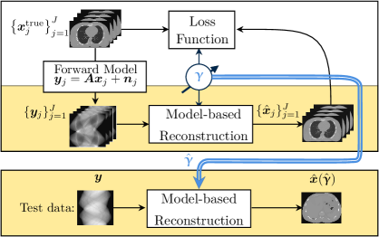
Figure 1.1: Depiction of a typical bilevel problem for image reconstruction, illustrated using XCAT phantom from [segars:10:4xp]. The upper box represents the training process, with the upper-level loss and lower-level cost function. During training, one minimizes the upper-level loss with respect to a vector of parameters, $\bm{\upgamma}$, that are used in the image reconstruction task. Once learned, $\hat{{\bm{\upgamma}}}$ is typically deployed in the same image reconstruction task, shown in the lower box.

We write the lower-level cost as an optimization problem with “argmin” and thus implicitly assume that $\Upphi$ has unique minimizer, ${\bm{\hat{x}}}$. The lower-level is guaranteed to have a unique minimizer when $\Upphi$ is a strictly convex function of ${\bm{x}}$. (See Section 4 for more discussion of this point). More generally, there may be a set of lower-level minimizers, each having some possibly distinct upper-level loss function value. For more discussion, [dempe:2003:annotatedbibliographybilevel] defines optimistic and pessimistic versions of the bilevel problem for the case of multiple lower-level solutions.

Bilevel methods typically use training data. Specifically, one often assumes that a given set of $J$ good quality images ${\bm{x}}^{\text{true}}_{1},\ldots,{\bm{x}}^{\text{true}}_{J}\in\mathbb{F}^{N}$ are representative of the images of interest in a given application. (For simplicity of notation we assume the training images have the same size, but they can have different sizes in practice.) We typically generate corresponding simulated measurements for each training image using the imaging system model:

$${\bm{y}}_{j}={\bm{A}}{\bm{x}}^{\text{true}}_{j}+{\bm{n}}_{j},\quad j=1,\ldots,J,$$ (1.4)

where ${\bm{n}}_{j}\in\mathbb{F}^{M}$ denotes an appropriate random noise realization. In (1.4), we add one noise realization to each of the $J$ images; in practice one could add multiple noise realizations to each ${\bm{x}}^{\text{true}}_{j}$ to augment the training data. We then use the training pairs $({\bm{x}}^{\text{true}}_{j},{\bm{y}}_{j})$ to learn a good value of $\bm{\upgamma}$. After those parameters are learned, we reconstruct subsequent test images using (1.3) with the learned hyperparameters $\hat{{\bm{\upgamma}}}$.

An alternative to the upper-level formulation (UL) is the following stochastic formulation of bilevel learning:

$$\hat{{\bm{\upgamma}}}=\operatorname*{argmin}_{{\bm{\upgamma}}\in\mathbb{F}^{R}} \underbrace{\mathbb{E}\left[\ell({\bm{\upgamma}})\right]}_{\approx\frac{1}{J}\sum_{j=1}^{J}\ell({\bm{\upgamma}}\,;\,{\bm{\hat{x}}}_{j}({\bm{\upgamma}}))}$$ (1.5)

where $${\bm{\hat{x}}}_{j}({\bm{\upgamma}})=\operatorname*{argmin}_{{\bm{x}}\in\mathbb{F}^{N}}\Upphi({\bm{x}}\,;{\bm{\upgamma}},{\bm{y}}_{j}).$$ (1.6)

The expectation, taken with respect to the training data and noise distributions, is typically approximated as a sample mean over $J$ training examples.

The definition of bilevel methods used in (UL) is not universal in the literature. In some works, bilevel methods refer to nested optimization problems with two levels, even when the two levels result from reformulating a single-level problem, e.g., [poon:2021:smoothbilevelprogramming]. That definition is much more encompassing, and includes primal-dual reformulations, Lagrangian reformulations of constrained optimization problems, and alternating methods that introduce then minimize over an auxiliary variable.

Another term in the literature, sometimes used interchangeably with a bilevel problem, is a mathematical program with equilibrium constraints (MPEC). As shown in Section 4, many bilevel optimization methods start by transforming the two-level problem into an equivalent single-level problem by replacing the lower-level optimization with a set of constraints based on optimally conditions. Bilevel problems are thus a subset of MPECs. MPECs are generally challenging due to their non-convex nature; even when the lower-level cost function is convex, the upper-level loss function is rarely convex. Importantly, $\ell(\cdot,\cdot)$ is often convex with respect to both arguments. However, $\ell({\bm{\upgamma}})=\ell({\bm{\upgamma}}\,;{\bm{\hat{x}}}({\bm{\upgamma}}))$ is generally non-convex in $\bm{\upgamma}$ due to how the lower-level minimizer depends on $\bm{\upgamma}$. There is a large literature on MPEC problems, e.g., [fletcher:2002:numericalexperiencesolving, colson:2007:overviewbileveloptimization, dempe:2003:annotatedbibliographybilevel], and on non-convex optimization more generally [jain:17:nco]. Bilevel methods are one sub-field in this large literature.

1.3 Running Example

To offer a concrete example, this review will frequently refer to the following running example (Ex), a filter learning bilevel problem:

$$\hat{{\bm{\upgamma}}} =\operatorname*{argmin}_{{\bm{\upgamma}}\in\mathbb{F}^{R}}\dfrac{1}{2}\|{\bm{\hat{x}}}({\bm{\upgamma}})-{\bm{x}}^{\text{true}}\|^{2}_{2},\text{ where }$$

$${\bm{\hat{x}}}({\bm{\upgamma}}) =\operatorname*{argmin}_{{\bm{x}}\in\mathbb{F}^{N}}\dfrac{1}{2}\left\lVert{\bm{A}}{\bm{x}}-{\bm{y}}\right\rVert^{2}_{2}+e^{\beta_{0}}\sum_{k=1}^{K}e^{\beta_{k}}{\bm{1}}^{\prime}\phi.({\bm{c}}_{k}\circledast{\bm{x}};\epsilon),$$ (Ex)

where ${\bm{\upgamma}}\in\mathbb{F}^{R}$ contains all variables that we wish to learn: the filter coefficients ${\bm{c}}_{k}\in\mathbb{F}^{S}$ and tuning parameters $\beta_{k}\in\mathbb{R}$ for all $k\in[1,K]$. We include an auxiliary tuning parameter, $\beta_{0}\in\mathbb{R}$, for easier comparison to other models. Fig. 1.2 depicts the running example and Fig. 1.3 shows example learned filters for a toy training image. Ref. [effland:2020:variationalnetworksoptimal] demonstrates how a spectral analysis of learned filters and penalty functions can be interpreted to provide insight into real-world problems.

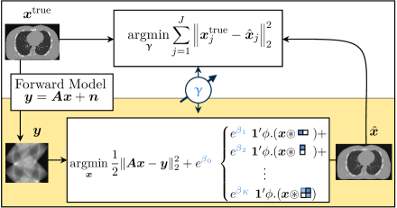
Figure 1.2: Bilevel problem in (Ex). The vector of learnable hyperparameters, $\bm{\upgamma}$, includes the tuning parameters, $\beta_{k}$, and the filter coefficients, ${\bm{c}}_{k}$, shown as example filters. Although this review will generally consider learning filters of a single size, the figure depicts how the framework easily extends to 2d filters of different sizes.

The learnable hyperparameters can also include the sparsifying function $\phi$, its corner rounding parameter $\epsilon$, the forward model $\bm{A}$, or some aspect of the data-fit term. For example, [haber:2003:learningregularizationfunctionals, effland:2020:variationalnetworksoptimal] learn the regularization functional and [ehrhardt:2021:inexactderivativefreeoptimization, sherry:2020:learningsamplingpattern] learn part of the forward model. Such examples are relatively rare in the bilevel methods literature to date.

Unlike many learning problems (see examples in Section 7.4), the running example (Ex) does not include any constraints on $\bm{\upgamma}$. Learned filters should be those that are best at the given task, where “best” is defined by the upper-level loss function. Therefore, a zero mean or norm constraint is not generally required, though some authors have found such constraints helpful, e.g., [kobler:2021:totaldeepvariation, chen:2014:insightsanalysisoperator]. Following previous literature, e.g., [samuel:2009:learningoptimizedmap], the tuning parameters in (Ex) are written in terms of an exponential function to ensure positivity. One could re-write (Ex) without this exponentiation “trick” and then add a non-negativity constraint to the upper-level problem; most of the methods discussed in this review generalize to this common variation by substituting gradient methods for projected gradient methods.

In (Ex), we drop the sum over $J$ training images for simplicity; the methods easily extend to multiple training signals. For ease of notation, we further simplify by considering ${\bm{c}}_{k}$ to be of length $S$ for all $k$, e.g., a 2D filter might be $\sqrt{S}\times\sqrt{S}$. In practice, the filters may be of different lengths with minimal impact on the methods presented in this review.

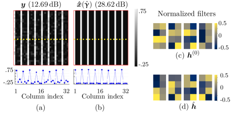
Figure 1.3: Example learned filters for a simple training image, normalized for easier visualization. The true image is zero-mean and repeats three columns of signal value $\text{-}0.25$ and one column of signal value $0.75$. (a) Noisy image. The lower plot shows a profile of one row of the image (marked by a dotted line). The signal-to-noise ratio, as defined in (3.2), is given in parenthesis. (b) The denoised image using learned filters as in (Ex). (c) Randomly initialized filters for the bilevel method ($K=4$ and $S=4\cdot 2$). (d) Corresponding learned filters. As expected based on the training image, the learned filters primarily involve vertical differences. Appendix D.1 provides further details including the regularization strength of each learned filter.

The function $\phi$ in (Ex) is a sparsity-promoting function. If we were to choose $\phi(z)=|z|$, then the regularizer would involve 1-norm terms of the type common in compressed sensing formulations:

$${\bm{1}}^{\prime}\phi.({\bm{c}}_{k}\circledast{\bm{x}})=\left\lVert{\bm{c}}_{k}\circledast{\bm{x}}\right\rVert_{1}.$$

However, to satisfy differentiability assumptions (see Section 4), this review will often consider $\phi$ to denote the following “corner rounded” 1-norm having the shape of a hyperbola with the corresponding first and second derivative:

$$\phi(z) =\sqrt{z^{2}+\epsilon^{2}}$$ (CR1N)

$${{\dot{\phi}}}(z) =\frac{z}{\sqrt{z^{2}+\epsilon^{2}}}\in[0,1)$$

$${\ddot{\phi}}(z) =\frac{\epsilon^{2}}{\left(z^{2}+\epsilon^{2}\right)^{3/2}}\in(0,\frac{1}{\epsilon}],$$

where $\epsilon$ is a small, relative to the expected range of $z$, parameter that controls the amount of corner rounding. (Here, we use a dot over the function rather than $\nabla$ to indicate a derivative because $\phi$ has a scalar argument.)

1.4 Conclusion

Bilevel methods for selecting hyperparameters offer many benefits. Previous papers motivate them as a principled way to approach hyperparameter optimization [holler:2018:bilevelapproachparameter, dempe:2020:bileveloptimizationadvances], as a task-based approach to learning [peyre:2011:learninganalysissparsity, haber:2003:learningregularizationfunctionals, delosreyes:2017:bilevelparameterlearning], and/or as a way to combine the data-driven improvements from learning methods with the theoretical guarantees and explainability provided by cost function-based approaches [chen:2021:learnabledescentalgorithm, calatroni:2017:bilevelapproacheslearning, kobler:2021:totaldeepvariation]. A corresponding drawback of bilevel methods are their computational cost; see Sections 4 and 5 for further discussion.

The task-based nature of bilevel methods is a particularly important advantage; Section 7.4 exemplifies why by comparing the bilevel problem to single-level, non-task-based approaches for learning sparsifying filters. Task-based refers to the hyperparameters being learned based on how well they work in the lower-level cost function–the image reconstruction task in our running example. The learned hyperparameters can also adapt to the training dataset and noise characteristics. The task-based nature yields other benefits, such as making constraints or regularizers on the hyperparameters generally unnecessary; Section 6.2 presents some exceptions and [dempe:2020:bileveloptimizationadvances] further discusses bilevel methods for applications with constraints.

There are three main elements to a bilevel approach. First, the lower-level cost function in a bilevel problem defines a goal, such as image reconstruction, including what hyperparameters can be learned, such as filters for a sparsifying regularizer. Section 2 provides background on this element specifically for image reconstruction tasks, such as the one in (Ex). Section 6.1 reviews example cost functions used in bilevel methods.

Second, the upper-level loss function determines how the hyperparameters should be learned. While the squared error loss function in the running example is a common choice, Section 3 discusses other loss functions based on supervised and unsupervised image quality metrics. Section 6.2 then reviews example loss functions used in bilevel methods.

While less apparent in the written optimization problem, the third main element for a bilevel problem is the optimization approach, especially for the upper-level problem. Section 3.2 briefly discusses various hyperparameter optimization strategies, then Sections 4 and 5 present multiple gradient-based bilevel optimization strategies. Throughout the review, we refer to the running example to show how the bilevel optimization strategies apply.

Chapter 2 Background: Cost Functions and Image Reconstruction

This review focuses on bilevel problems having image reconstruction as the lower-level problem. Image reconstruction involves undoing any transformations inherent in an imaging system, e.g., a camera or CT scanner, and removing measurement noise, e.g., thermal and shot noise, to realize an image that captures an underlying object of interest, e.g., a patient’s anatomy. Fig. 2.1 shows an example image reconstruction pipeline for CT data. The following sections formally define image reconstruction, discuss why regularization is important, and overview common approaches to regularization.

2.1 Image Reconstruction

Although the true object is in continuous space, image reconstruction is almost always performed on sampled, discretized signals [lewitt:03:oom]. Without going into detail of the discretization process, we define ${\bm{x}}^{\text{true}}\in\mathbb{F}^{N}$ as the “true,” discrete signal. The goal of image reconstruction is to recover an estimate ${\bm{\hat{x}}}\approx{\bm{x}}^{\text{true}}$ given corrupted measurements ${\bm{y}}\in\mathbb{F}^{M}$. Although we define the signal as a one-dimensional vector for notational convenience, the mathematics generalize to arbitrary dimensions.

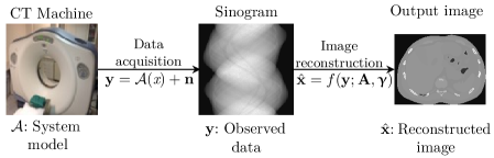
Figure 2.1: Example image reconstruction pipe-line, illustrated using XCAT phantom from [segars:10:4xp]. Here $\mathcal{A}$ denotes the actual physical mapping of the imaging system and $\bm{A}$ denotes the numerical system matrix used for reconstruction.

To find ${\bm{\hat{x}}}$, image reconstruction involves minimizing a cost function, $\Upphi({\bm{x}}\,;{\bm{\upgamma}})$, with two terms:

$${\bm{\hat{x}}}=\operatorname*{argmin}_{{\bm{x}}\in\mathbb{F}^{N}}\underbrace{\overbrace{d({\bm{x}}\,;{\bm{y}})}^{\text{Data-fit}}+\;\;\;\beta\overbrace{R({\bm{x}}\,;{\bm{\upgamma}})}^{\text{Regularizer}}}_{\Upphi({\bm{x}}\,;{\bm{\upgamma}})}$$ (2.1)

The first term, $d({\bm{x}}\,;{\bm{y}})$, is a data-fit term that captures the physics of the ideal (noiseless) system using the matrix ${\bm{A}}\in\mathbb{F}^{M\times N}$; that matrix models the physical system such that we expect an observation, $\bm{y}$, to be ${\bm{y}}\approx{\bm{A}}{\bm{x}}$.

The most common data-fit term penalizes the square Euclidean norm of the “measurement error,” $d({\bm{x}}\,;{\bm{y}})=\left\lVert{\bm{A}}{\bm{x}}-{\bm{y}}\right\rVert^{2}_{2}$. This intuitive data-fit term can be derived from a maximum likelihood perspective, assuming a white Gaussian noise distribution [elad:07:avs]. Using the system model (1.4) and assuming the noise is normally distributed with zero-mean and variance $\sigma^{2}$, the maximum likelihood estimate ${\bm{\hat{x}}}_{\text{MLE}}$ is the image that is most likely given the observation $\bm{y}$, i.e.,

$${\bm{\hat{x}}}_{\text{MLE}} =\operatorname*{argmax}_{{\bm{x}}\in\mathbb{F}^{N}}\text{Prob}({\bm{x}}\,;\,{\bm{y}},\sigma^{2}).$$

Substituting the assumed Gaussian distribution (and ignoring constants independent of $\bm{x}$),

$${\bm{\hat{x}}}_{\text{MLE}} =\operatorname*{argmax}_{{\bm{x}}\in\mathbb{F}^{N}}e^{\frac{\text{-}1}{2\sigma^{2}}\left\lVert{\bm{A}}{\bm{x}}-{\bm{y}}\right\rVert^{2}}=\operatorname*{argmin}_{{\bm{x}}\in\mathbb{F}^{N}}\dfrac{1}{2}\left\lVert{\bm{A}}{\bm{x}}-{\bm{y}}\right\rVert^{2}={\bm{A}}^{+}{\bm{y}},$$

where ${\bm{A}}^{+}$ is the pseudo-inverse of $\bm{A}$.

The regularization term in (2.1) can be motivated by maximum a posteriori probability (MAP) estimation [elad:07:avs]. Rather than maximizing the likelihood of $\bm{x}$, the MAP estimate ${\bm{\hat{x}}}_{\text{MAP}}$ maximizes the conditional probability of $\bm{x}$ given the observation $\bm{y}$

$${\bm{\hat{x}}}_{\text{MAP}} =\operatorname*{argmax}_{{\bm{x}}\in\mathbb{F}^{N}}\text{Prob}({\bm{x}}|{\bm{y}})$$

$$=\operatorname*{argmax}_{{\bm{x}}\in\mathbb{F}^{N}}\text{Prob}({\bm{y}}|{\bm{x}})\text{Prob}({\bm{x}})$$

by Bayes theorem. A MAP estimator requires assuming a prior distribution on $\bm{x}$. Taking the logarithm and substituting the assumed Gaussian distribution for $\text{Prob}({\bm{y}}|{\bm{x}}\,;\,\sigma^{2})$ yields

$${\bm{\hat{x}}}_{\text{MAP}} =\operatorname*{argmin}_{{\bm{x}}\in\mathbb{F}^{N}}\frac{1}{2\sigma^{2}}\left\lVert{\bm{A}}{\bm{x}}-{\bm{y}}\right\rVert^{2}-\text{log}\left(\text{Prob}({\bm{x}})\right),$$

where the regularization term in (2.1) comes from the log probability of $\bm{x}$, i.e., the two are equivalent when one assumes the probability model $\text{Prob}({\bm{x}})=\frac{1}{Z({\bm{\upgamma}})}\exp\{-R({\bm{x}}\,;\,{\bm{\upgamma}})\}$, where $Z({\bm{\upgamma}})$ is a scalar such that the probability integrates to one. The MLE estimate is equivalent to the MAP estimate when the prior on $\bm{x}$ is an (unbounded) “uniform” distribution.

While MAP estimation provides a useful perspective, common regularizers do not correspond to proper probability models. Further, the connection between the regularization perspective and the Bayesian perspective is simplest when the parameters $\bm{\upgamma}$ are given. To learn $\bm{\upgamma}$, Bayesian formulations must consider the partition function $Z({\bm{\upgamma}})$; that complication is avoided for bilevel formulations using a regularized lower-level problem.

Many image reconstruction problems have linear system models. In image denoising problems, one takes ${\bm{A}}=\bm{I}$. For image inpainting, $\bm{A}$ is a diagonal matrix of 1’s and 0’s, where the 0’s correspond to sample indices of missing data [guillemot:14:iio]. In MRI, the system matrix is often approximated as a diagonal matrix times a discrete Fourier transform matrix, though more accurate models are often needed [fessler:10:mbi]. In some settings, one can learn $\bm{A}$ [golub:80:aao], or at least parts of $\bm{A}$ [ying:07:jir], as part of the estimation process. Although the bilevel method generalizes to learning $\bm{A}$, the majority of papers in the field assume $\bm{A}$ is known; Section 6 discusses a few exceptions.

Using the system model (1.4), if $\bm{n}$ were known and $\bm{A}$ were invertible, we could simply compute ${\bm{\hat{x}}}={\bm{x}}^{\text{true}}={\bm{A}}^{\text{-}1}({\bm{y}}-{\bm{n}})$. However, $\bm{n}$ is random and, while we may be able to model its characteristics, we never know it exactly. Further, the system matrix, $\bm{A}$, is often not invertible because the reconstruction problem is frequently under-determined, with fewer knowns than unknowns ($M<N$). Therefore, we must include prior assumptions about ${\bm{x}}^{\text{true}}$ to make the problem feasible. These assumptions about ${\bm{x}}^{\text{true}}$ are captured in the second, regularization term in (2.1), which depends on $\bm{\upgamma}$. The following section further discusses regularizers.

In sum, image reconstruction involves finding ${\bm{\hat{x}}}$ that matches the collected data and satisfies a set of prior assumptions. The data-fit term encourages ${\bm{\hat{x}}}$ to be a good match for the data; without this term, there would be no need to collect data. The regularization term encourages ${\bm{\hat{x}}}$ to match the prior assumptions. Finally, the tuning parameter, $\beta$, controls the relative importance of the two terms. The cost function can be minimized using different optimization techniques depending on the form of each term.

This section is a very short overview of image reconstruction methods. See [mccann:2019:biomedicalimagereconstruction] for a more thorough review of biomedical image reconstruction.

2.2 Sparsity-Based Regularizers

The regularization, or prior assumption, term in (2.1) often involves assumptions about sparsity [eldar:12:cs, chambolle:2016:introductioncontinuousoptimization]. The basic idea behind sparsity-based regularization is that the true signal is sparse in some representation, while the noise or corruption is not. Thus, one can use the representation to separate the noise and signal, and then keep only the sparse signal component. In fact, a known sparsifying representation for a signal can help to “reconstruct a signal from far fewer measurements than required by the Shannon-Nyquist sampling theorem” [chambolle:2016:introductioncontinuousoptimization].

The regularization design problem therefore requires determining what representation best sparsifies the signal. There are two main types of sparsity-based regularizers corresponding to two representational assumptions: synthesis and analysis [elad:07:avs, ravishankar:20:irf]; Fig. 2.2 depicts both. While both are popular, this review concentrates on analysis regularizers, which are more widely represented in the bilevel image reconstruction literature. This section briefly compares the analysis and synthesis formulations. Here we simplify the formulas by considering ${\bm{A}}=\bm{I}$; the discussion generalizes to reconstruction by including $\bm{A}$. For more thorough discussions of analysis and synthesis regularizers, see [elad:07:avs, nam:2013:cosparseanalysismodel, ravishankar:20:irf].

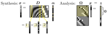
Figure 2.2: Depiction of synthesis and analysis sparsity. Under the synthesis model of sparsity (left), $\bm{x}$ is a linear combination of a few dictionary atoms. The dictionary, $\bm{D}$, is typically wide, with more atoms (columns) than elements in $\bm{x}$. Under the analysis model of sparsity (right), $\bm{x}$ is orthogonal to many filters. The filter matrix, $\bm{\Omega}$, is typically tall, with more filters (rows) than elements in $\bm{x}$.

2.2.1 Synthesis Regularizers

Synthesis regularizers model a signal being composed of building blocks, or “atoms.” Small subsets of the atoms span a low dimensional subspace and the sparsity assumption is that the signal requires using only a few of the atoms. More formally, the synthesis model is ${\bm{y}}={\bm{x}}+{\bm{n}}$, where the signal ${\bm{x}}={\bm{D}}{\bm{z}}$ and $\bm{z}$ is a sparse vector. The columns of ${\bm{D}}\in\mathbb{F}^{N\times K}$ contain contain the $K$ dictionary atoms and form a low dimensional subspace for the signal. If $\bm{D}$ is a wide matrix ($N<K$), the dictionary is over-complete and it is easier to represent a wide range of signals with a given number of dictionary atoms. The dictionary is complete when $\bm{D}$ is square (and full rank) and under-complete if $\bm{D}$ is tall (an uncommon choice).

Assuming one knows or has already learned $\bm{D}$, one can use the sparsity synthesis assumption to denoise a noisy signal $\bm{y}$ by optimizing

$${\bm{\hat{x}}}={\bm{D}}\cdot(\underbrace{\operatorname*{argmin}_{{\bm{z}}\in\mathbb{F}^{K}}\dfrac{1}{2}\left\lVert{\bm{D}}{\bm{z}}-{\bm{y}}\right\rVert^{2}+\bm{1}^{\prime}\phi.({\bm{z}})}_{\hat{{\bm{z}}}}).$$ (2.2)

The estimation procedure involves finding the sparse codes, $\hat{{\bm{z}}}$, from which the image is synthesized via ${\bm{\hat{x}}}={\bm{D}}\hat{{\bm{z}}}$. Common sparsity-inducing functions, $\phi$, are the absolute value or a non-zero indicator function, equivalent to the 1-norm and 0-norm respectively. The 2-norm is occasionally used in the regularizer, but it does not yield true sparse codes and it over-penalizes large values [elad:10].

As written in (2.2), the synthesis formulation constrains the signal, $\bm{x}$, to be in the range of $\bm{D}$. This “strict synthesis” model can be undesirable in some applications, e.g., when one is not confident in the quality of the dictionary. An alternative formulation is

$${\bm{\hat{x}}} =\operatorname*{argmin}_{{\bm{x}}\in\mathbb{F}^{N}}\dfrac{1}{2}\left\lVert{\bm{x}}-{\bm{y}}\right\rVert^{2}+\beta R({\bm{x}}),$$

$$R({\bm{x}}) =\operatorname*{min}_{{\bm{z}}\in\mathbb{F}^{K}}\dfrac{1}{2}\left\lVert{\bm{x}}-{\bm{D}}{\bm{z}}\right\rVert^{2}+\bm{1}^{\prime}\phi.({\bm{z}}),$$ (2.3)

which no longer constrains $\bm{x}$ to be exactly in the range of $\bm{D}$. One can also learn $\bm{D}$ while solving (2.3) [peyre:11:aro].

Both synthesis denoising forms have equivalent sparsity constrained versions; one can replace $\bm{1}^{\prime}\phi.({\bm{z}})$ with a characteristic function that is 0 within some desired set and infinite outside it, e.g.,

$$\psi({\bm{z}})=\begin{cases}0&\text{ if }\left\lVert{\bm{z}}\right\rVert_{0}\leq\kappa\\ \infty&\text{ else, }\end{cases}$$ (2.4)

for some sparsity constraint given by the hyperparameter $\kappa\in\mathbb{N}$.

See [candes:2006:robustuncertaintyprinciples, elad:10] for discussions of when the synthesis model can guarantee accurate recovery of signals. The minimization problem in (2.3) is called sparse coding and is closely related to the LASSO problem [tibshirani:1996:regressionshrinkageselection]. One can think of the entire dictionary $\bm{D}$ as a hyperparameter that can be learned with a bilevel method [zhou:17:bmb].

2.2.2 Analysis Regularizers

Analysis regularizers model a signal as being sparsified when mapped into another vector space by a linear transformation, often represented by a set of filters. More formally, an analysis model assumes the signal satisfies ${\bm{\Omega}}{\bm{x}}={\bm{z}}$ for a sparse coefficient vector $\bm{z}$. Often the rows of the matrix ${\bm{\Omega}}\in\mathbb{F}^{K\times N}$ are thought of as filters and the rows of $\bm{\Omega}$ where $[{\bm{\Omega}}{\bm{x}}]_{k}=0$ span a subspace to which $\bm{x}$ is orthogonal. The analysis operator is called over-complete if $\bm{\Omega}$ is tall ($N<K$), complete if $\bm{\Omega}$ is square (and full rank), and under-complete if $\bm{\Omega}$ is wide.

A particularly common analysis regularizer is based on a discretized version of total variation (TV) [rudin:92:ntv], and uses finite difference filters (or, more generally, filters that approximate higher-order derivatives). The finite difference filters sparsify any piece-wise constant (flat) regions in the signal, leaving the edges that are often approximately sparse in natural images. Other common analysis regularizers include the discrete Fourier transform (DFT), curvelets, and wavelet transforms [candes:2011:compressedsensingcoherent].

The literature is less consistent in analysis regularizer vocabulary, and $\bm{\Omega}$ has been called an analysis dictionary, an analysis operator, a filter matrix, and a cosparse operator. The term “cosparse” comes from the sparsity holding in the codomain of the transformation $T\{{\bm{x}}\}={\bm{\Omega}}{\bm{x}}$. The cosparsity of $\bm{x}$ with respect to $\bm{\Omega}$ is the number of zeros in ${\bm{\Omega}}{\bm{x}}$ or $K-\left\lVert{\bm{\Omega}}{\bm{x}}\right\rVert_{0}$ [nam:2013:cosparseanalysismodel]. Correspondingly, “cosupport” describes the indices of the rows where ${\bm{\Omega}}{\bm{x}}=0$. We find the phrase “analysis operator” intuitive for general $\bm{\Omega}$’s and “filter matrix” more descriptive when referring to the specific (common) case when the rows of $\bm{\Omega}$ are dictated by a set of convolutional filters.

Assuming one knows, or has already learned, $\bm{\Omega}$, one can use the analysis sparsity assumption to denoise a noisy signal, $\bm{y}$, by optimizing

$${\bm{\hat{x}}}=\operatorname*{argmin}_{{\bm{x}}\in\mathbb{F}^{N}}\dfrac{1}{2}\left\lVert{\bm{x}}-{\bm{y}}\right\rVert^{2}+\beta\bm{1}^{\prime}\phi.({\bm{\Omega}}{\bm{x}}).$$ (2.5)

An alternative version is

$${\bm{\hat{x}}}=\operatorname*{argmin}_{{\bm{x}}\in\mathbb{F}^{N}}\dfrac{1}{2}\left\lVert{\bm{x}}-{\bm{y}}\right\rVert^{2}+\beta R({\bm{x}})$$ (2.6)

$$R({\bm{x}})=\operatorname*{min}_{{\bm{z}}\in\mathbb{F}^{K}}\dfrac{1}{2}\left\lVert{\bm{\Omega}}{\bm{x}}-{\bm{z}}\right\rVert^{2}+\bm{1}^{\prime}\phi.({\bm{z}}).$$

As in the synthesis case, both analysis formulations have equivalent sparsity-constrained forms using a characteristic function as in (2.4).

See [candes:2011:compressedsensingcoherent] for an error bound on the estimated signal ${\bm{\hat{x}}}$ when using a 1-norm as the regularization function.

2.2.3 Comparing Analysis and Synthesis Approaches

The analysis and synthesis models are equivalent when the dictionary and analysis operator are invertible, with ${\bm{D}}={\bm{\Omega}}^{\text{-}1}$ [elad:07:avs]. Furthermore, in the denoising scenario where the system matrix $\bm{A}$ is identity, the two are almost equivalent in the under-complete case, with the lack of full equivalence stemming from the analysis form not constraining $\bm{x}$ to be in the range space $\bm{D}$ [elad:07:avs].

As shown in [chambolle:2016:introductioncontinuousoptimization, Example 3.1], the analysis model can more generally be related to a Lasso-like problem using Legendre-Fenchel conjugates and convex duality. Appendix A briefly reviews duality and the main results from primal-dual analysis used throughout this review. Considering the analysis operator learning problem (2.5), when the sparsity promoting function $\phi$ is convex and $\phi(z)<\infty$ for some $z$, the dual problem corresponding to (2.5) is

$$\hat{{\bm{d}}}=\operatorname*{argmin}_{{\bm{d}}\in\mathbb{F}^{K}}\dfrac{1}{2}\left\lVert{\bm{\Omega}}^{\prime}{\bm{d}}-{\bm{y}}\right\rVert^{2}+\phi^{*}({\bm{d}}),$$

where ${\bm{d}}$ is the dual variable and $\phi^{*}$ is the conjugate function of $\phi$. (The primal solution ${\bm{\hat{x}}}$ can be computed from $\hat{{\bm{d}}}$ using (A.11).) This dual problem is similar in form to the inner minimization in the strict synthesis formulation (2.2). This relation between the analysis model and its dual formulation is limited to cases where $\phi$ is convex.

Whether analysis-based or synthesis-based regularizers are generally preferable is an open question, and the answer likely depends on the application and the relative importance of reconstruction accuracy and speed [elad:07:avs]. Synthesis regularization is perhaps easier to interpret because of its generative nature. In contrast, bilevel analysis filter learning is a discriminative learning approach: the task-based filters must learn to distinguish “good” and “bad” image features.

The synthesis approach used to be “widely considered to provide superior results” [elad:07:avs, 950]. However, [elad:07:avs] goes on to show that an analysis regularizer produced more accurate reconstructed images in experiments on real images. Later analysis-based results also show competitive, if not superior, quality results when compared to similar synthesis models [hawe:13:aol, ravishankar:2013:learningsparsifyingtransforms]. See [fessler:20:omf] for a survey of optimization methods for MRI reconstruction and a comparison of the computational challenges for cost functions with synthesis and analysis-based regularizers.

The analysis and synthesis regularizers in (2.2) and (2.6) quickly yield infeasibly large operators as the signal size increases. In practice, both approaches are usually implemented with patch-based formulations. For the synthesis approach, the patches typically overlap and there is an averaging effect. Analysis regularizers that have rows corresponding to filters, called the convolutional analysis model, extend very naturally to a global image regularizer. For example, in the lower-level cost function of our running filter learning example (Ex), we can define an analysis regularizer matrix as follows:

$${\bm{\Omega}}=\begin{bmatrix}{\bm{C}}_{1}\\ \vdots\\ {\bm{C}}_{K}\end{bmatrix}\in\mathbb{F}^{KN\times N}.$$ (2.7)

Imposing this convolutional structure on $\bm{\Omega}$ helps make learning problems feasible as one only has to learn the $S$ coefficients of each of the $K$ filters rather than learning the full $\bm{\Omega}$ matrix. This structure also ensures translation invariance of the regularizer. See [chen:2014:insightsanalysisoperator] and [pfister:2019:learningfilterbank] for discussion of the connections between global models and patch-based models for analysis regularizers. The running example in this survey focuses on bilevel learning of convolutional analysis regularizers.

2.3 Brief History of Analysis Regularizer Learning

In 2003, haber:2003:learningregularizationfunctionals proposed using bilevel methods to learn part of the regularizer in inverse problems. The authors motivate the use of bilevel methods through the task-based nature, noting that “the choice of good regularization operators strongly depends on the forward problem.” They consider learning tuning parameters, space-varying weights, and regularization operators (comparable to defining $\phi$), all for regularizers based on penalizing the energy in the derivatives of the reconstructed image. Their framework is general enough to handle learning filters. Ref. [haber:2003:learningregularizationfunctionals] was published a few years earlier than the other bilevel methods we consider in this review and was not cited in most other early works; [afkham:2021:learningregularizationparameters] calls it a “groundbreaking, but often overlooked publication.”

In 2005, roth:2005:fieldsexpertsframework proposed the Field of Experts (FoE) model to learn filters. Although the FoE is not formulated as a bilevel method, many papers on bilevel methods for filter learning cite FoE as a starting or comparison point. The FoE model is a translation-invariant analysis operator model, built on convolutional filters. It is motivated by the local operators and presented as a Markov random field model, with the order of the field determined by the filter size.

Under the FoE model, the negative log of the probability of a full image, $\bm{x}$, is proportional to

$$\sum_{k}\beta_{k}\;\phi.({\bm{c}}_{k}\circledast{\bm{x}})\text{ where }\phi(z)=\text{log}\left(1+\dfrac{1}{2}z^{2}\right).$$ (2.8)

This (non-convex) choice of sparsity function $\phi$ stems from the Student-t distribution. Ref. [roth:2005:fieldsexpertsframework] learns the filters and filter-dependent tuning parameters such that the model distribution is as close as possible (defined using Kullback-Leibler divergence) to the training data distribution.

In 2007, tappen:2007:learninggaussianconditional proposed a different model based on convolutional filters: the Gaussian Conditional Random Field (GCRF) model. Rather than using a sparsity promoting regularizer, the GCRF uses a quadratic function for $\phi$. The authors introduce space-varying weights, $\bm{W}$, so that the quadratic model does not overly penalize sharp features in the image. The general idea behind ${\bm{W}}$ is to use the given (noisy) image to guess where edges occur, and correspondingly penalize those areas less to avoid blurring edges. The likelihood for GCRF model is thus (to within a proportionality constant and monotonic function transformations):

$$\sum_{k}\left\lVert{\bm{c}}_{k}\circledast{\bm{x}}-e_{k}\{{\bm{x}}\}\right\rVert^{2}_{{\bm{W}}_{k}},$$

where the term $e_{k}\{{\bm{x}}\}$ captures the estimated value of the filtered image. For example, [tappen:2007:learninggaussianconditional] used one averaging filter and multiple differencing filters for the ${\bm{c}}_{k}$’s. The corresponding estimated values are $\bm{x}$ for the averaging filter and zero for the differencing filters.

The filters, ${\bm{c}}_{k}$, are pre-determined in the GCRF model; the learned element is how to form the weights as a function of image features. Specifically, each ${\bm{W}}_{k}$ is formed as a linear combination of the (absolute) responses to a set of edge-detecting filters, with the linear combination coefficients learned from training data. Rather than maximizing the likelihood of training data as in [roth:2005:fieldsexpertsframework], [tappen:2007:learninggaussianconditional] learns these coefficients to minimize the (corner-rounded) $l_{1}$ norm of the error of the predicted image, which is a form of bilevel learning even though not described with that terminology.

Apparently one of the first papers to explicitly propose using bilevel methods to learn filters appeared in 2009, where samuel:2009:learningoptimizedmap considered a bilevel formulation where the upper-level loss was the squared Euclidean norm of training data and the lower-level cost was a denoising task based on filter sparsity equivalent to (Ex). The method builds on the FoE model, using the same $\phi$ as in [roth:2005:fieldsexpertsframework], but now learning the filters using a bilevel formulation rather than by maximizing a likelihood.

In 2011, peyre:2011:learninganalysissparsity proposed a similar bilevel method to learn analysis regularizers. The authors generalized the denoising task to use an analysis operator matrix and a wider class of sparsifying functions. Their results concentrate on the convolutional filter case with a corner-rounded 1-norm for $\phi$.

Both [samuel:2009:learningoptimizedmap] and [peyre:2011:learninganalysissparsity] focus on introducing the bilevel method for analysis regularizer learning, with denoising or inpainting as illustrations. Section 4 further discusses the methodology of both papers. Many of the bilevel based papers in this review build on one or both of their efforts. The rest of the review will summarize other bilevel based papers; here, we highlight some of papers in the non-bilevel thread of the literature for context and comparison.

ophir:2011:sequentialminimaleigenvalues proposed another approach to learning an analysis operator. The method learns the operator one row at a time by searching for vectors orthogonal to the training signals. Algorithm parameters were chosen empirically without an upper-level loss function as a guide.

Between 2011 [yaghoobi:2011:analysisoperatorlearning] and 2013 [yaghoobi:2013:constrainedovercompleteanalysis], yaghoobi:2011:analysisoperatorlearning were among the first to formally present analysis operator learning as an optimization problem. Their conference paper [yaghoobi:2011:analysisoperatorlearning] considered noiseless training data and proposed learning an analysis operator as

$$\operatorname*{argmin}_{\bm{\Omega}}\|{\bm{\Omega}}{\bm{X}}^{\text{true}}\|_{1}\text{ s.t. }{\bm{\Omega}}\in\mathcal{S}$$ (2.9)

for some constrained set $\mathcal{S}$. Each column of ${\bm{X}}^{\text{true}}\in\mathbb{F}^{N\times J}$ contains a training sample. The authors discussed varying options for $\mathcal{S}$, including a row norm, full rank, and tight frame constrained set.

Without any constraint on $\bm{\Omega}$, the trivial solution to (2.9) would be to learn the zero matrix, which is not informative for any problem such as image denoising. Section 7.4 discusses in more detail the need for constraints and the various constraint options proposed for filter learning.

Ref. [yaghoobi:2013:constrainedovercompleteanalysis] extends (2.9) to the noisy case where one does not have access to ${\bm{X}}^{\text{true}}$. The proposed cost function is

$$\operatorname*{argmin}_{{\bm{\Omega}},\,{\bm{X}}}\left\lVert{\bm{\Omega}}{\bm{X}}\right\rVert_{1}+\frac{\beta}{2}\left\lVert{\bm{X}}-{\bm{Y}}\right\rVert^{2}\text{ s.t. }{\bm{\Omega}}\in\mathcal{S},$$ (2.10)

where each column of $\bm{Y}$ contains a noisy data vector. Ref. [yaghoobi:2013:constrainedovercompleteanalysis] minimized (2.10) by alternating updating $\bm{X}$, using alternating direction method of multipliers (ADMM), and $\bm{\Omega}$, using a projected subgradient method for various constraint sets $\mathcal{S}$, especially Parseval tight frames.

In the same time-frame, kunisch:2013:bileveloptimizationapproach started to analyze the theory behind the bilevel problem, building off the ideas in [samuel:2009:learningoptimizedmap, peyre:2011:learninganalysissparsity]. Among the theoretical analysis, [kunisch:2013:bileveloptimizationapproach] proves the existence of upper-level minimizers when the bilevel problem takes the form of (Ex), $\bm{\upgamma}$ is the tuning parameters (the $\beta_{k}$ values), and $\phi$ corresponds to the squared 2-norm or the 1-norm. When $\phi(z)=z^{2}$, there is an analytic solution to the lower-level problem and a corresponding closed-form solution to the gradient of the upper-level problem; [kunisch:2013:bileveloptimizationapproach] uses this fact to discuss qualitative properties of the minimizer. Ref. [kunisch:2013:bileveloptimizationapproach] also proposed an efficient semi-smooth Newton algorithm for finding $\hat{{\bm{\upgamma}}}$ (using corner rounding for the 1-norm case) and used this algorithm to make empirical comparisons of multiple sparsifying functions (2-norm, 1-norm, and $p=1/2$-norm) and different pre-defined filter banks.

Also in 2013, ravishankar:2013:learningsparsifyingtransforms made a distinction between the analysis model, where one models ${\bm{y}}={\bm{x}}+{\bm{n}}$ with ${\bm{z}}={\bm{\Omega}}{\bm{x}}$ being sparse, and the transform model, where ${\bm{\Omega}}{\bm{y}}={\bm{z}}+{\bm{n}}$ where $\bm{z}$ is sparse. The analysis version models the measurement as being a cosparse signal plus noise; the transform version models the measurement as being approximately cosparse. Another perspective on the distinction is that, if there is no noise, the analysis model constrains $\bm{y}$ to be in the range space of $\bm{\Omega}$, while there is no such constraint on the transform model. The corresponding transform learning problem is

$$\operatorname*{argmin}_{{\bm{\Omega}}}\operatorname*{min}_{\bm{Z}}\left\lVert{\bm{\Omega}}{\bm{Y}}-{\bm{Z}}\right\rVert^{2}_{2}+ R({\bm{\Omega}})\quad\text{ s.t. }\left\lVert{\bm{Z}}_{i}\right\rVert_{0}\leq\alpha\;\forall i,$$ (2.11)

where $i$ indexes the columns of $\bm{Z}$. Ref. [ravishankar:2013:learningsparsifyingtransforms] considers only square matrices $\bm{\Omega}$. The regularizer, $R$, promotes diversity in the rows of $\bm{\Omega}$ to avoid trivial solutions, similar to the set constraint in (2.10).

A more recent development is directly modeling the convolutional structure during the learning process. In 2020, [chun:2020:convolutionalanalysisoperator] proposed Convolutional Analysis Operator Learning (CAOL) to learn convolutional filters without patches. The CAOL cost function is

$$\operatorname*{argmin}_{[{\bm{c}}_{1},\ldots,{\bm{c}}_{K}]}\sum_{k=1}^{K}\operatorname*{min}_{\bm{z}}\dfrac{1}{2}\left\lVert{\bm{c}}_{k}\circledast{\bm{x}}-{\bm{z}}\right\rVert^{2}_{2}+\beta\left\lVert{\bm{z}}\right\rVert_{0}\text{ s.t. }[{\bm{c}}_{1}\ldots{\bm{c}}_{K}]\in\mathcal{S}.$$ (2.12)

Unlike the previous cost functions, which typically require patches, CAOL can easily handle full-sized training images $\bm{x}$ due to the nature of the convolutional operator.

While model-based methods were being developed in the signal processing literature, convolutional neural network (CNN) models were being advanced and trained in the machine learning and computer vision literature [haykin:96:nne] [hwang:97:tpp] [lucas:18:udn]. The filters used in CNN models like U-Nets [ronneberger:15:unc] can be thought of as having analysis roles in the earlier layers, and synthesis roles in the final layers [ye:18:dcf]. See also [wen:20:tlf] for further connections between analysis and transform models within CNN models. CNN training is usually supervised, and the supervised approach of bilevel learning of filters strengthens the relationships between the two approaches. A key distinction is that CNN models are generally feed-forward computations, whereas bilevel methods of the form (LL) have a cost function formulation. See Section 7 for further discussion of the parallels between CNNs and bilevel methods.

2.4 Summary

This background section focused on the lower-level problem: image reconstruction with a sparsity-based regularizer. After defining the problem and the need for regularization, Section 2.3 reviewed the history of analysis regularizer learning and included many examples of methods to learn hyperparameters.

Bilevel methods are just one, task-based way to learn such hyperparameters. Section 7.4 further expands on this point, but we can already see benefits of the task-based nature of bilevel methods. Without the bilevel approach, filters are often learned such that they best sparsify training data. These sparsifying filters can then be used in a regularizer for image reconstruction tasks. However, they are learned to sparsify, not necessarily to best reconstruct. In contrast, the bilevel approach aims to learn filters that best reconstruct images (or whatever other task is desired), even if those filters are not the ones that best sparsify. Although this distinction may seem subtle, [chambolle:2021:learningconsistentdiscretizations] shows that different filters work better for image denoising versus image inpainting.

Having provided some background on the lower-level cost function and motivated bilevel methods, this review now turns to defining the upper-level loss function and surveying methods of hyperparameter optimization.

Chapter 3 Background: Loss Functions and
Hyperparameter Optimization

Most inverse problems involve at least one hyperparameter. For example, the general reconstruction cost function (2.1) requires choosing the tuning parameter $\beta$ that trades-off the influence of the data-fit and regularization terms. The field of hyperparameter optimization is large and encompasses categorical hyperparameters, such as which optimizer to use; conditional hyperparameters, where certain hyperparameters are relevant only if others take on certain values; and integer or real-valued hyperparameters [feurer:2019:chapterhyperparameteroptimization]. Here, we focus on learning real-valued, continuous hyperparameters.

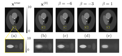
Figure 3.1: Example reconstructed simulated MRI images that demonstrate the importance of tuning parameters. (a) The original image, ${\bm{x}}^{\text{true}}\in R^{N}$, is a SheppLogan phantom [shepp:74:tfr] and $N$ is the number of pixels. (b) A simplistic reconstruction $\frac{1}{N}{\bm{A}}^{\prime}{\bm{y}}$ of the noisy, undersampled data, $\bm{y}$. This image is used as initialization, ${\bm{x}}^{(0)}$, for the following reconstructions. (c-e) Reconstructed images, found by optimizing $\operatorname*{argmin}_{\bm{x}}\dfrac{1}{2}\|{\bm{A}}{\bm{x}}-{\bm{y}}\|^{2}_{2}+10^{\beta}N\phi({\bm{C}}{\bm{x}})$, where $\bm{C}$ is an operator that takes vertical and horizontal finite differences. The reconstructed images correspond to (c) $\beta=-6$, resulting in an image that contains ringing artifacts, (d) $\beta=-3$, resulting in a visually appealing ${\bm{\hat{x}}}$, and (e) $\beta=1$, resulting in a blurred image. The demonstration code and more details about the reconstruction set-up are available on github [fessler:2020:mirtdemo01recon].

A hyperparameter’s value can greatly influence the properties of the minimizer and a tuned hyperparameter typically improves over a default setting [feurer:2019:chapterhyperparameteroptimization]. Fig. 3.1 illustrates how changing a tuning parameter can dramatically impact the visual quality of the reconstructed image. If $\beta$ is too low, not enough weight is on the regularization term, and the minimizer is likely to be corrupted by noise in the measurements. If $\beta$ is too high, the regularization term dominates, and the minimizer will not align with the measurements.

Generalizing to an arbitrary learning problem that could have multiple hyperparameters, the goal of hyperparameter optimization is to find the “best” set of hyperparameters, $\hat{{\bm{\upgamma}}}$, to meet a goal, described by a loss function $\ell$. Specifically, we wish to solve

$$\hat{{\bm{\upgamma}}}=\operatorname*{argmin}_{{\bm{\upgamma}}\in\Gamma}\mathbb{E}\left[\ell({\bm{\upgamma}})\right],$$ (3.1)

where $\Gamma$ is the set of all possible hyperparameters and the expectation is taken with respect to the distribution of the input data. If evaluating $\ell$ uses the output of another optimization problem, e.g., ${\bm{\hat{x}}}$, then (3.1) is a bilevel problem as defined in (UL).

There are two key tasks in hyperparameter optimization.

1. The first is to quantify how good a hyperparameter is; this step is equivalent to defining $\ell$ in (3.1). Section 3.1 focuses on a high-level discussion of loss functions in the broader image quality assessment (IQA) literature. Section 6.2 builds on this discussion by reviewing specific loss functions used in bilevel methods.

2. The second step is finding a good hyperparameter, which is equivalent to designing an optimization algorithm to minimize (3.1). Section 3.2 introduces common approaches, all of which have computational requirements that scale at least linearly with the number of hyperparameters. This scaling quickly becomes infeasible for large $\bm{\upgamma}$, which motivates the focus on gradient-based bilevel methods in the remainder of this review.

The next two sections address each of these tasks in turn.

3.1 Image Quality Metrics

This section concentrates on the part of the upper-level loss function that compares the reconstructed image, ${\bm{\hat{x}}}({\bm{\upgamma}})$, to the true image, ${\bm{x}}^{\text{true}}$. As mentioned in Section 1, bilevel methods rarely require additional regularization for $\bm{\upgamma}$, but it is simple to add a regularization term to any of the loss functions if useful for a specific application. To discuss only the portion of the loss function that measures image quality, we use the notation $\ell({\bm{\upgamma}}\,;{\bm{\hat{x}}}({\bm{\upgamma}}))=l({\bm{\hat{x}}},\,{\bm{x}}^{\text{true}})$.

Picking a loss function is part of the engineering design process. No single loss function is likely to work in all scenarios; users must decide on the loss function that best fits their system, data, and goals. Consequently, there are a wide variety of loss functions proposed in the literature and some approaches combine multiple loss functions [you:2018:structuresensitivemultiscaledeep, hammernik:2020:machinelearningimage].

One important decision criteria when selecting a loss function is the end purpose of the image. Much of the IQA literature focuses on metrics for images of natural scenes and is often motivated by applications where human enjoyment is the end-goal [wang:2004:imagequalityassessment, wang:2011:reducednoreferenceimage]. In contrast, in the medical image reconstruction field, image quality is not the end-goal, but rather a means to achieving a correct diagnosis. Thus, the perceptual quality is less important than the information content.

There are two major classes of image quality metrics in the IQA literature, called full-reference and no-reference IQA. The principles are somewhat analogous to supervised and unsupervised approaches in the machine learning literature. This section discusses some of the most common full-reference and no-reference loss functions; see [zhang:2012:comprehensiveevaluationfull] for a comparison of 11 full-reference IQA metrics and [zhang:2020:blindimagequality] for additional no-reference IQA metrics.

Perhaps surprisingly, the bilevel filter learning literature contains few examples of loss functions other than squared error or slight variants (see Section 6.2). While this is likely at least partially due to the computational requirements of bilevel methods (see Section 4 and 5), exploring additional loss functions is an interesting future direction for bilevel research.

3.1.1 Full-Reference IQA

Full-reference IQA metrics assume that you have a noiseless image, ${\bm{x}}^{\text{true}}$, for comparison. Some of the simplest (and most common) full-reference loss functions are:

• Mean squared error (MSE or $\ell_{2}$ error):

  $$l_{\mathrm{MSE}}({\bm{\hat{x}}},{\bm{x}}^{\text{true}})=\frac{1}{N}\left\lVert{\bm{\hat{x}}}-{\bm{x}}^{\text{true}}\right\rVert^{2}_{2}$$

• Mean absolute error (or $\ell_{1}$ error): $l_{\mathrm{MAE}}({\bm{\hat{x}}},{\bm{x}}^{\text{true}})=\frac{1}{N}\left\lVert{\bm{\hat{x}}}-{\bm{x}}^{\text{true}}\right\rVert_{1}$

• Signal to Noise Ratio (SNR, commonly expressed in dB):
  

  $$l_{\mathrm{SNR}}({\bm{\hat{x}}},{\bm{x}}^{\text{true}})=10\text{log}\left(\frac{\left\lVert{\bm{x}}^{\text{true}}\right\rVert^{2}_{2}}{\left\lVert{\bm{\hat{x}}}-{\bm{x}}^{\text{true}}\right\rVert^{2}_{2}}\right)$$ (3.2)

• Peak SNR (PSNR, in dB): $l_{\mathrm{PSNR}}({\bm{\hat{x}}},{\bm{x}}^{\text{true}})=10\text{log}\left(\frac{N\left\lVert{\bm{x}}^{\text{true}}\right\rVert_{\infty}}{\left\lVert{\bm{\hat{x}}}-{\bm{x}}^{\text{true}}\right\rVert^{2}_{2}}\right)$.

The Euclidean norm is also frequently used as the data-fit term for reconstruction.

MSE (and the related metrics SNR and PSNR) are common in the signal processing field; they are intuitive and easy to use because they are differentiable and operate point-wise. However, these measures do not align well with human perceptions of image quality [mason:2020:comparisonobjectiveimage, zhang:2012:comprehensiveevaluationfull]. For example, scaling an image by 2 leads to the same visual quality but causes 100% MSE. Fig. 3.2 shows a clean image and five images with different degradations. All five degraded images have almost equivalent squared errors, but humans judge their qualities as very different.

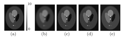
Figure 3.2: Example distortions that yield images with identical normalized squared error values: $\left\lVert{\bm{x}}^{\text{true}}-{\bm{x}}\right\rVert/\left\lVert{\bm{x}}^{\text{true}}\right\rVert=0.17$. (a) The original image, ${\bm{x}}^{\text{true}}$, is a SheppLogan phantom [shepp:74:tfr]. The remaining images are displayed with the same colormap and have the following distortions: (b) blurred with an averaging filter, (c) additive, white Gaussian noise, (d) salt and pepper noise, and (e) a constant value added to every pixel.

Tuning parameters using MSE as the loss function tends to lead to images that are overly-smoothed, sacrificing high frequency information [gholizadehansari:20:dlf, seif:18:ebl]. High frequency details are particularly important for perceptual quality as they correspond to edges in images. Therefore, some authors use the MSE on edge-enhanced versions of images to discourage solutions that blur edges. For example, [ravishankar:2011:mrimagereconstruction] used a “high frequency error norm” metric consisting of the MSE of the difference of ${\bm{\hat{x}}}$ and ${\bm{x}}^{\text{true}}$ after applying a Laplacian of Gaussian (LoG) filter.

Another common full-reference IQA is Structural SIMilarity (SSIM) [wang:2004:imagequalityassessment] that attempts to address the issues with MSE discussed above. SSIM is defined in terms of the local luminance, contrast, and structure in images. A multiscale extension of SSIM, called MS-SSIM, considers these features at multiple resolutions [wang:2003:multiscalestructuralsimilarity]. The method computes the contrast and structure measures of SSIM for downsampled versions of the input images and then defines MS-SSIM as the product of the luminance at the original scale and the contrast and structure measures at each scale. However, SSIM and MS-SSIM may not correlate well with human observer performance on radiological tasks [renieblas:17:ssi].

Recent works, e.g., [bosse:2018:deepneuralnetworks, zhang:2020:blindimagequality], consider using (deep) CNN models for IQA. CNN methods are increasingly popular and their use as a model for the human visual system [lindsay:2020:convolutionalneuralnetworks] makes them an attractive tool for assessing images. For example, [bosse:2018:deepneuralnetworks] proposed a CNN with convolutional and pooling layers for feature extraction and fully connected layers for regression. They used VGG [simonyan:2015:verydeepconvolutional], a frequently-cited CNN design with $3\times 3$ convolutional kernels, as the basis of the feature extraction portion of their network. Ref. [bosse:2018:deepneuralnetworks] showed that deeper networks with more learnable parameters were able to better predict image quality. However, datasets of images with quality labels remain relatively scarce, making it difficult to train deep networks.

3.1.2 No-reference IQA

No-reference, or unsupervised, IQA metrics attempt to quantify an image’s quality without access to a noiseless version of the image. These metrics rely on modeling statistical characteristics of images or noise. Many no-reference IQA metrics assume the noise distribution is known.

The discrepancy principle is a classic example of an IQA metric that uses an assumed noise distribution to characterize the expected relation between the reconstructed image and the noisy data. For additive zero-mean white Gaussian noise with known variance $\sigma^{2}$, the discrepancy principle uses the fact that the expected MSE in the data space is the noise variance [phillips:62:atf]:

$$\mathbb{E}\left[\frac{1}{M}\left\lVert{\bm{A}}{\bm{\hat{x}}}({\bm{\upgamma}})-{\bm{y}}\right\rVert^{2}_{2}\right]=\sigma^{2}.$$

The discrepancy principle can be used as a stopping criteria in machine learning methods or as a loss function, e.g.,

$$\ell({\bm{\upgamma}}\,;{\bm{\hat{x}}}({\bm{\upgamma}}))=\left(\frac{1}{M}\left\lVert{\bm{A}}{\bm{\hat{x}}}({\bm{\upgamma}})-{\bm{y}}\right\rVert^{2}_{2}-\sigma^{2}\right)^{2}.$$

However, images of varying quality can yield the same noise estimate, as seen in Fig. 3.2. Related methods have been developed for Poisson noise as well [hebert:92:sbm].

Paralleling MSE’s popularity among supervised loss metrics, Stein’s Unbiased Risk Estimator (SURE) [stein:1981:estimationmeanmultivariate] is an unbiased estimate of MSE that does not require noiseless images. Let ${\bm{y}}={\bm{x}}^{\text{true}}+{\bm{n}}$ denote a signal plus noise measurement where $\bm{n}$ is, as above, Gaussian noise with known variance $\sigma^{2}$. The SURE estimate of the MSE of a denoised signal, ${\bm{\hat{x}}}$, is

$$\frac{1}{N}\left\lVert{\bm{\hat{x}}}({\bm{y}})-{\bm{y}}\right\rVert^{2}_{2}-\sigma^{2}+\frac{2\sigma^{2}}{N}\mathrm{Tr}\left(\nabla_{y}{\bm{\hat{x}}}({\bm{y}})\right),$$ (3.3)

where we write ${\bm{\hat{x}}}$ as a function of $\bm{y}$ to emphasize the dependence and $\mathrm{Tr}\left(\cdot\right)$ denotes the trace operation. For large signal dimensions $N$, such as is common in image reconstruction problems, the law of large numbers suggests SURE is a fairly accurate approximation of the true MSE.

It is often impractical to evaluate the divergence term in (3.3), due to computational limitations or not knowing the form of ${\bm{\hat{x}}}({\bm{y}})$. A Monte-Carlo approach to estimating the divergence [ramani:2008:montecarlosureblackbox] uses the following key equation:

$$\mathrm{Tr}\left(\nabla_{\bm{y}}{\bm{\hat{x}}}({\bm{y}})\right)=\lim_{\epsilon\rightarrow 0}\mathbb{E}\left[{\bm{b}}^{\prime}\cdot\frac{{\bm{\hat{x}}}({\bm{y}}+\epsilon{\bm{b}})-{\bm{\hat{x}}}({\bm{y}})}{\epsilon}\right],$$ (3.4)

where $\bm{b}$ is a independent and identically distributed (i.i.d.) random vector with zero mean, unit variance, and bounded higher order moments. Theoretical and empirical arguments show that a single noise vector can well-approximate the divergence [ramani:2008:montecarlosureblackbox], so only two calls to the lower-level solver ${\bm{\hat{x}}}({\bm{y}})$ are required. This method treats the lower-level problem like a blackbox, thus allowing one to estimate the divergence of complicated functions, including those that may not be differentiable.

See [soltanayev:2018:trainingdeeplearning, kim:20:uto, zhussip:19:tdl] for examples of applying the Monte-Carlo estimation of SURE to train deep neural networks, and [zhang:2020:bilevelnestedsparse, deledalle:2014:steinunbiasedgradient] for two examples of learning a tuning parameter using a bilevel approach with SURE as the upper-level loss function. For extensions to inverse problems (where ${\bm{A}}\neq\bm{I})$ and to noise from exponential families, see [eldar:08:rbe, eldar:2009:generalizedsureexponential, giryes:11:tpg].

While SURE and the discrepancy principle are popular no-reference metrics in the signal processing literature, there are many additional no-reference metrics in the image quality assessment literature. These metrics typically depend on modeling one (or more) of three things [wang:2011:reducednoreferenceimage]:

• image source characteristics,

• image distortion characteristics, e.g., blocking artifact from JPEG compression, and/or

• human visual system perceptual characteristics.

As an example of a strategy that can capture both image source and human visual system characteristics, natural scene statistics characterize the distribution of various features in natural scenes, typically using some filters [mittal:2013:makingcompletelyblind, wang:2011:reducednoreferenceimage]. If a feature reliably follows a specific statistical pattern in natural images but has a noticeably different distribution in distorted images, one can use that feature to assign quality scores to images. Some IQA metrics attempt to first identify the type of distortion and measure features specific to that distortion, while others use the same features for all images.

In addition to their use in full-reference IQA, CNN models have be trained to perform no-reference IQA [kang:2014:convolutionalneuralnetworks, bosse:2018:deepneuralnetworks]. For example, [kang:2014:convolutionalneuralnetworks] proposes a CNN model that extracts small ($32\times 32$) patches from images, estimates the quality of each one, and averages the scores over all patches to get a quality score for the entire image. Briefly, their method involves local contrast normalization for each patch, applying (learned) convolutional filters to extract features, maximum and minimum pooling, and fully connected layers with rectified linear units (ReLUs). As with most no-reference IQAs, [kang:2014:convolutionalneuralnetworks] trained their CNN on a dataset of human encoded image quality scores (see [laboratoryforimagevideoengineering::imagevideoquality] for a commonly used collection of publicly available test images with quality scores). Unlike most other IQA approaches, [kang:2014:convolutionalneuralnetworks] used backpropagation to learn all the CNN weights rather than learning a transformation from handcrafted features to quality scores.

Interestingly, some of the no-reference IQA metrics [mittal:2013:makingcompletelyblind, kang:2014:convolutionalneuralnetworks, wang:2011:reducednoreferenceimage] approach the performance of the full-reference IQAs in terms of their ability to match human judgements of image quality. This observation suggests that there is room to improve full-reference IQA metrics and that assessing image quality is a very challenging problem!

3.2 Parameter Search Strategies

After selecting a metric to measure how good a hyperparameter is, the next task is devising a strategy to find the best hyperparameter according to that metric. Search strategies fall into three main categories: (i) model-free, $\ell$-only; (ii) model-based, $\ell$-only; and (iii) gradient-based, using both $\ell$ and $\nabla\ell$. Model-free strategies do not assume any information about about the hyperparameter landscape, whereas model-based strategies use historical $\ell$ evaluations to predict the loss function at untested hyperparameter values.

The following sections describe common model-free and model-based hyperparameter search strategies that only use $\ell$. See [dempe:2020:bileveloptimizationadvances, Ch. 13 and Ch. 20.6] for discussion of additional gradient-free methods for bilevel problems, e.g., population-based evolutionary algorithms, and [larson:2019:derivativefreeoptimizationmethods] for a general discussion of derivative-free optimization methods.

The third class of hyperparameter optimization schemes are approaches based on gradient descent of a bilevel problem. The high-level strategy in bilevel approaches is to calculate the gradient of the upper-level loss function $\ell$ with respect to $\bm{\upgamma}$ and then use any gradient descent method to minimize $\bm{\upgamma}$. Although this approach can be computationally challenging, it generalizes well to a large number of hyperparameters. Section 4 and Section 5 discuss this point further and go into depth on different methods for computing this gradient.

3.2.1 Model-free Hyperparameter Optimization

The most common search strategy is probably an empirical search, where a researcher tries different hyperparameter combinations manually. A punny, but often accurate, term for this manual search is GSD: grad[uate] student descent [gencoglu:2019:harksidedeep]. bergstra:12:rsf hypothesized that manual search is common because it provides some insight as the user must evaluate each option, it requires no overhead for implementation, and it can perform reliably in very low dimensional hyperparameter spaces.

Grid search is a more systematic alternative to manual search. When there are only one or two continuous hyperparameters, or the possible set of hyperparameters, ${\bm{\Gamma}}$, is small, a grid search (or exhaustive search) strategy may suffice to find the optimal value, $\hat{{\bm{\upgamma}}}$, to within the grid spacing. However, the complexity of grid search grows exponentially with the number of hyperparameters. Regularizers frequently have many hyperparameters, so one generally requires a more sophisticated search strategy.

One popular approach is random search, which [bergstra:12:rsf] shows is superior to a grid search, especially when some hyperparameters are more important than others. There are also variations on random search, such as using Poisson disk sampling theory to explore the hyperparameter space [muniraju:18:crs]. The simplicity of random search makes it popular, and, even if one uses a more complicated search strategy, random search can provide a useful baseline or an initialization strategy. However, random search, like grid search, suffers from the curse of dimensionality, and is less effective as the hyperparameter space grows.

Another group of model-free blackbox strategies are population-based methods such as evolutionary algorithms. A popular population-based method is the covariance matrix adaption evolutionary strategy (CMA-ES) [beyer:2001:theoryevolutionstrategies]. In short, every iteration, CMA-ES involves sampling a multivariate normal distribution to create a number of “offspring” samples. Mimicking natural selection, these offspring are judged according to some fitness function, a parallel to the upper-level loss function. The fittest offspring determine the update to the normal distribution and thus “pass on” their good characteristics to the next generation.

3.2.2 Model-based Hyperparameter Optimization

Model-based search strategies assume a model (or prior) for the hyperparameter space and use only loss function evaluations (no gradients). This section discusses two common model-based strategies: Bayesian methods and trust region methods.

Bayesian methods fit previous hyperparameter trials’ results to a model to select the hyperparameters that appear most promising to evaluate next [klein:17:fbh]. For example, a common model for the hyperparameters is the Gaussian Process prior. Given a few hyperparameter and cost function points, a Bayesian method involves the following steps.

1. Find the mean and covariance functions for the Gaussian Process. The mean function will generally interpolate the sampled points. The covariance function is generally expressed as a kernel function, often using squared exponential functions [frazier:2018:tutorialbayesianoptimization].

2. Create an acquisition function. The acquisition function captures how desirable it is to sample (“acquire”) a hyperparameter setting. Thus, it should be large (desirable) for hyperparameter values that are predicted to yield small loss function values or that have high enough uncertainty that they may yield low losses. The design of the acquisition function thus trades-off between exploring new areas of the hyperparameter landscape with high uncertainty and a more locally focused exploitation of the current best hyperparameter settings. See [frazier:2018:tutorialbayesianoptimization] for a discussion of specific acquisition function designs.

3. Maximize the acquisition function (typically designed to be easy to optimize) to determine which hyperparameter point to sample next.

4. Evaluate the loss function at the new hyperparameter candidate.

These steps repeat for a given amount of time or until convergence.

The derivative-free, trust-region method (TRM) [conn:2000:trustregionmethods] is similar to Bayesian optimization in that it involves fitting an easier to optimize function to the loss function of interest, $\ell$, and then minimizing the easier, surrogate function (the “model”). The “trust-region” in TRM captures how well the model matches the observed $\ell$ values and determines the maximum step at every iteration, typically by comparing the actual decrease in $\ell$ (based on observed function evaluations) to the predicted decrease (based on the model).

TRM requires only function evaluations, not gradients, to construct and then minimize the model. However, unlike most Bayesian optimization-based approaches, TRM uses a local (often quadratic) model for $\ell$ around the current iterate, rather than a surrogate that fits all previous points. In taking a step based on this local information, TRM resembles gradient-based approaches.

Following the methods from [ehrhardt:2021:inexactderivativefreeoptimization], who assume an additively separable and quadratic upper-level loss function, e.g.,

$$\ell({\bm{\upgamma}})=\frac{1}{J}\sum_{j=1}^{J}\ell({\bm{\upgamma}}\,;{\bm{\hat{x}}}_{j}({\bm{\upgamma}}))=\frac{1}{J}\sum_{j=1}^{J}(\underbrace{{\bm{\hat{x}}}_{j}({\bm{\upgamma}})-{\bm{x}}^{\text{true}}_{j}}_{r_{j}({\bm{\upgamma}}\,;{\bm{\hat{x}}}_{j}({\bm{\upgamma}})})^{2},$$

an outline for a TRM is

1. Create a quadratic model for the upper-level loss function.

   1. Select a set of upper-level interpolating points and (approximately) evaluate $r$ at each one. After an initialization, one can generally reuse samples from previous iterations. Ref. [ehrhardt:2021:inexactderivativefreeoptimization] discusses requirements on the interpolation set to guarantee a good geometry and conditions for re-setting the interpolation sample.

   2. Estimate the gradients of $r_{j}$ by interpolating a set of $R$ samples (recall ${\bm{\upgamma}}\in\mathbb{F}^{R}$) of the upper-level loss function. This requires solving a set of $R$ linear equations in $R$ unknowns.

   3. Model the upper-level by replacing $r_{j}$ with its tangent-plane approximation: $r_{j}({\bm{\upgamma}}+\delta)\approx r({\bm{\upgamma}})+(\tilde{\nabla}r_{j}({\bm{\upgamma}}))^{\prime}\delta$, where $\tilde{\nabla}r_{j}({\bm{\upgamma}})$ is the estimated gradient from the previous step.

2. Minimize the model within some trust region to find the next candidate set of upper-level parameters. By construction, this is a simple convex-constrained quadratic problem.

3. Accept or reject the updated parameters and update the trust region. If the ratio between the actual reduction and predicted reduction is low, the model may no longer be a good fit, the update is rejected, and the trust region shrinks.

Recall that evaluating $\ell$ is typically expensive in bilevel problems as each upper-level function evaluation involves optimizing the lower-level cost. Thus, even constructing the model for a TRM can be expensive. To mitigate this computational complexity, [ehrhardt:2021:inexactderivativefreeoptimization] incorporated a dynamic accuracy component, with the accuracy for the lower-level cost initially set relatively loose (leading to rough estimates of $\ell$) but increasing with the upper-level iterations (leading to refined estimates of $\ell$ as the algorithm nears a stationary point).

A main result from [ehrhardt:2021:inexactderivativefreeoptimization] is a bound on the number of iterations to reach an $\epsilon$-optimal point (defined as $\operatorname*{min}_{u}\|\nabla_{\bm{\upgamma}}\ell({{\bm{\upgamma}}^{(u)}})\|<\epsilon$, where $u$ indexes the upper-level iterates). The bound derivation assumes (i) $\Upphi$ is differentiable in $\bm{x}$, (ii) $\Upphi$ is $\mu$-strongly convex, i.e., $\Upphi({\bm{x}})-\frac{\mu}{2}\left\lVert{\bm{x}}\right\rVert^{2}$ is convex for $\mu>0$, (iii) the derivative of $\Upphi$ is Lipschitz continuous, and (iv) the first and second derivative of the lower-level cost with respect to $\bm{x}$ exist and are continuous. These requirements are satisfied by the example filter learning problem (Ex), when $\bm{A}$ has full column rank, and more generally when there are certain constraints on the hyperparameters. The iteration bound is a function of the following:

• the tolerance $\epsilon$,

• the trust region parameters (parameters that control the increase and decrease in trust region size based on the actual to predicted reduction, the starting trust region size, and the minimum possible trust region size),

• the initialization for $\bm{\upgamma}$, and

• the maximum possible error between the gradient of the upper-level loss function and the gradient of the model for the upper-level loss within a trust region (when the gradient of $\ell$ is Lipschitz continuous, this bound is the corresponding Lipschitz constant).

The number of iterations required to reach such an $\epsilon$-optimal point is $\mathcal{O}\!\left(\frac{1}{\epsilon^{2}}\right)$ [ehrhardt:2021:inexactderivativefreeoptimization] and the number of required upper-level loss function evaluations depends more than linearly on $R$ [roberts:2021:inexactdfobilevel]. The growth with the number of hyperparameters impedes its use in problems with many hyperparameters. However, new techniques such as [cartis:2021:scalablesubspacemethods] may be able to decrease or remove the dependency, making TRMs promising alternatives to the gradient-based bilevel methods described in the remainder of this review.

3.3 Summary

Turning from the discussion of the lower-level problem in Section 2, this section concentrated on the other two aspects of bilevel problems: the upper-level loss function and the optimization strategy.

The loss function defines what a “good” hyperparameter is, typically using a metric of image quality to compare ${\bm{\hat{x}}}({\bm{\upgamma}})$ to a clean, training image, ${\bm{x}}^{\text{true}}$. Variations on squared error are the most common upper-level loss functions. Section 3.1 discussed many other full-reference and no-reference options, including ones motivated by human judgements of perceptual quality, from the image quality assessment literature; Section 6.2 gives examples of bilevel methods that use some of these other loss functions.

The second half of this section concentrated on model-free and model-based hyperparameter search strategies. The grid search, CMA-ES, and trust region methods described above all scale at least linearly with the number of hyperparameters. Similarly, Bayesian optimization is best-suited for small hyperparameter dimensions; [frazier:2018:tutorialbayesianoptimization] suggests it is typically used for problems with 20 or fewer hyperparameters.

The remainder of this review considers gradient-based strategies for hyperparameter optimization. The main benefit of gradient-based methods is that they can scale to the large number of hyperparameters that are commonly used in machine learning applications. Correspondingly, the main drawbacks of a gradient-based method over the methods discussed in this section are the implementation complexity, the per-iteration computational complexity, and the differentiability requirement. Sections 4 and 5 discuss multiple options for gradient-based methods.

Chapter 4 Gradient-Based Bilevel Methodology:
The Groundwork

When the lower-level optimization problem (LL) has a closed-form solution, ${\bm{\hat{x}}}$, one can substitute that solution into the upper-level loss function (UL). In this case, the bilevel problem is equivalent to a single-level problem and one can use classic single-level optimization methods to minimize the upper-level loss. (See [kunisch:2013:bileveloptimizationapproach] for analysis and discussion of some simple bilevel problems with closed-form solutions for ${\bm{\hat{x}}}$.) This review focuses on the more typical bilevel problems that lack a closed-form solution for ${\bm{\hat{x}}}$.

Although there are a wide variety of optimization methods for this challenging category of bilevel problems, many methods are built on gradient descent of the upper-level loss. The primary challenge with gradient-based methods is that the gradient of the upper-level function depends on a variable that is itself the solution to an optimization problem involving the hyperparameters of interest. This section describes two common approaches for overcoming this challenge. The first approach uses the fact that the gradient of the lower-level cost function is zero at the minimizer to compute an exact gradient at the exact minimizer. The second approach uses knowledge of the update scheme for the lower-level cost function to calculate the exact gradient for an approximation to the minimizer after a specific number of lower-level optimization steps.

With this (approximation of the) gradient of the lower-level optimization variable with respect to the hyperparameters, one can compute the gradient of the upper-level loss function with respect to the hyperparameters, $\bm{\upgamma}$. Section 5 uses the building blocks from this section to explain various bilevel methods based on this gradient.

4.1 Set-up

Recall from Section 1.2 that a generic bilevel problem is

$$\operatorname*{argmin}_{\bm{\upgamma}}\; \ell({\bm{\upgamma}}\,;{\bm{\hat{x}}}({\bm{\upgamma}}))\text{ where }{\bm{\hat{x}}}({\bm{\upgamma}})=\operatorname*{argmin}_{{\bm{x}}}\Upphi({\bm{x}}\,;{\bm{\upgamma}}).$$ (4.1)

For simplicity, hereafter we focus on the case $\mathbb{F}=\mathbb{R}$. Using the chain rule, the gradient of the upper-level loss function with respect to the hyperparameters is

$$\nabla\ell({\bm{\upgamma}}) =\nabla_{\bm{\upgamma}}\ell({\bm{\upgamma}}\,;{\bm{\hat{x}}}({\bm{\upgamma}}))+\left(\nabla_{\bm{\upgamma}}{\bm{\hat{x}}}({\bm{\upgamma}})\right)^{\prime}\nabla_{\bm{x}}\ell({\bm{\upgamma}}\,;{\bm{\hat{x}}}({\bm{\upgamma}})),$$ (4.2)

where on the right hand side $\nabla_{\bm{\upgamma}}$ and $\nabla_{\bm{x}}$ denote partial derivatives w.r.t. the first and second arguments of $\ell({\bm{\upgamma}}\,;\,{\bm{x}})$, respectively. We typically select the loss function such that it is easy to compute these partials. For example, if $\ell$ is the squared error training loss, i.e., $\ell({\bm{\upgamma}}\,;{\bm{\hat{x}}}({\bm{\upgamma}}))=\frac{1}{2}\left\lVert{\bm{\hat{x}}}({\bm{\upgamma}})-{\bm{x}}^{\text{true}}\right\rVert^{2}_{2}$, then

$$\nabla_{\bm{\upgamma}}\ell({\bm{\upgamma}}\,;{\bm{\hat{x}}}({\bm{\upgamma}}))=0\text{ and }\nabla_{\bm{x}}\ell({\bm{\upgamma}}\,;{\bm{\hat{x}}}({\bm{\upgamma}}))={\bm{\hat{x}}}({\bm{\upgamma}})-{\bm{x}}^{\text{true}}.$$

The following sections survey methods to find the remaining, more challenging piece in (4.2): the Jacobian $\nabla_{\bm{\upgamma}}{\bm{\hat{x}}}({\bm{\upgamma}})\in\mathbb{F}^{N\times R}$ for a given value of $\bm{\upgamma}$.

4.2 Minimizer Approach

The first approach finds the Jacobian $\nabla_{\bm{\upgamma}}{\bm{\hat{x}}}({\bm{\upgamma}})$ by assuming the gradient of $\Upphi$ at the minimizer is zero. There are two ways to arrive at the final expression: the implicit function theorem (IFT) perspective (as in [samuel:2009:learningoptimizedmap, gould:2016:differentiatingparameterizedargmin]) and the Lagrangian/KKT transformation perspective (as in [chen:2014:insightsanalysisoperator, holler:2018:bilevelapproachparameter]). This section presents both perspectives in sequence. The end of the section summarizes the required assumptions and discusses computational complexity and memory requirements.

The first step in both perspectives is to assume we have computed ${\bm{\hat{x}}}({\bm{\upgamma}})$ and that the lower-level problem 4.1 is unconstrained (e.g., no non-negativity or box constraints). Therefore, the gradient of $\Upphi$ with respect to $\bm{x}$ and evaluated at ${\bm{\hat{x}}}$ must be zero:

$$\nabla_{\bm{x}}\Upphi({\bm{x}}\,;{\bm{\upgamma}})\bigg{\rvert}_{{\bm{x}}={\bm{\hat{x}}}({\bm{\upgamma}})}=\nabla_{\bm{x}}\Upphi({\bm{\hat{x}}}\,;{\bm{\upgamma}})=\bm{0}.$$ (4.3)

After this point, the two perspectives diverge.

4.2.1 Implicit Function Theorem Perspective

In the IFT perspective, we apply the IFT (cf. [fessler:96:mav]) to define a function $h$ such that ${\bm{\hat{x}}}({\bm{\upgamma}})=h({\bm{y}},{\bm{\upgamma}})$. If we could write $h$ explicitly, then the bilevel problem could be converted to an equivalent single-level problem. However, per the IFT, we do not need to define $h$, we only state that such an $h$ exists. Combining this definition with (4.3) yields

$$\bm{0} =\nabla_{{\bm{x}}}\Upphi(h({\bm{y}},{\bm{\upgamma}});{\bm{\upgamma}}).$$ (4.4)

Using the chain rule, we differentiate both sides of (4.4) with respect to $\bm{\upgamma}$. The $\bm{I}$ in the equation below follows from the chain rule because $\nabla_{\bm{\upgamma}}{\bm{\upgamma}}=\bm{I}$. We then rearrange terms to solve for the desired quantity, noting that $\nabla_{\bm{\upgamma}}{\bm{\hat{x}}}({\bm{\upgamma}})=\nabla_{\bm{\upgamma}}h({\bm{y}},{\bm{\upgamma}})$. Thus, evaluating all terms at ${\bm{\hat{x}}}$ leads to the Jacobian expression of interest:

$$0= \nabla_{{\bm{x}}{\bm{x}}}\Upphi(h({\bm{y}},{\bm{\upgamma}});{\bm{\upgamma}})\nabla_{\bm{\upgamma}}h({\bm{y}},{\bm{\upgamma}})+\bm{I}\cdot\nabla_{{\bm{x}}{\bm{\upgamma}}}\Upphi(h({\bm{y}},{\bm{\upgamma}});{\bm{\upgamma}})$$

$$\nabla_{\bm{\upgamma}}h({\bm{y}},{\bm{\upgamma}})= -[\nabla_{{\bm{x}}{\bm{x}}}\Upphi(h({\bm{y}},{\bm{\upgamma}});{\bm{\upgamma}})]^{-1}\cdot\nabla_{{\bm{x}}{\bm{\upgamma}}}\Upphi(h({\bm{y}},{\bm{\upgamma}});{\bm{\upgamma}})$$

$$\nabla_{\bm{\upgamma}}{\bm{\hat{x}}}({\bm{\upgamma}})= -[\nabla_{{\bm{x}}{\bm{x}}}\Upphi({\bm{\hat{x}}};{\bm{\upgamma}})]^{-1}\cdot\nabla_{{\bm{x}}{\bm{\upgamma}}}\Upphi({\bm{\hat{x}}};{\bm{\upgamma}}).$$ (4.5)

When $\Upphi$ is strictly convex, the Hessian of $\Upphi$ is positive definite and $\nabla_{{\bm{x}}{\bm{x}}}\Upphi({\bm{\hat{x}}};{\bm{\upgamma}})$ is invertible.

Substituting (4.5) into (4.2) yields the following expression for the gradient of the upper-level loss function with respect to $\bm{\upgamma}$:

$$\nabla\ell({\bm{\upgamma}}) =\nabla_{\bm{\upgamma}}\ell({\bm{\upgamma}}\,;{\bm{\hat{x}}}({\bm{\upgamma}}))-\left(\nabla_{{\bm{x}}{\bm{\upgamma}}}\Upphi({\bm{\hat{x}}};{\bm{\upgamma}})\right)^{\prime}{\left(\nabla_{{\bm{x}}{\bm{x}}}\Upphi\left({\bm{\hat{x}}}\,;{\bm{\upgamma}}\right)\right)^{\text{-}1}}\nabla_{\bm{x}}\ell({\bm{\upgamma}}\,;{\bm{\hat{x}}}).$$

If there is a closed-form solution to the lower-level problem, one can verify that the IFT gradient agrees with the analytic gradient; see [gould:2016:differentiatingparameterizedargmin] for examples.

4.2.2 KKT Conditions

In the Lagrangian perspective, (4.3) is treated as a constraint on the upper-level problem, creating a single-level problem with $N$ equality constraints:

$$\operatorname*{argmin}_{\bm{\upgamma}}\ell({\bm{\upgamma}}\,;{\bm{x}})\text{ subject to }\nabla_{\bm{x}}\Upphi({\bm{x}}\,;{\bm{\upgamma}})={\bm{0}}_{N}.$$ (4.6)

Using the KKT conditions to transform the bilevel problem into a single-level, constrained problem is sometimes called the “KKT transformation” of the bilevel problem. This transformation relates bilevel optimization to mathematical programs with equilibrium constraints (MPEC); see [dempe:2020:bileveloptimizationadvances, Ch. 12] and some authors use approaches from the broader MPEC literature to approach bilevel problems [hintermuller:2015:bileveloptimizationcalibrating]. The Lagrangian corresponding to (4.6) is

$$L({\bm{x}},{\bm{\upgamma}},{\bm{\nu}}) =\ell({\bm{\upgamma}}\,;{\bm{x}})+{\bm{\nu}}^{T}\nabla_{\bm{x}}\Upphi({\bm{x}}\,;{\bm{\upgamma}})$$

where ${\bm{\nu}}\in\mathbb{F}^{N}$ is a vector of Lagrange multipliers associated with the $N$ equality constraints in (4.6).

The Lagrange reformulation is generally well-posed because many bilevel problems, such as (Ex), satisfy the linear independence constraint qualification (LICQ) [dempe:2003:annotatedbibliographybilevel, scholtes:2001:howstringentlinear]. The LICQ requires that the matrix of derivatives of the constraint has full row rank [scholtes:2001:howstringentlinear], i.e.,

$$\text{rank}\left(\begin{bmatrix}\nabla_{{\bm{x}}{\bm{\upgamma}}}\Upphi({\bm{x}}\,;{\bm{\upgamma}})&\nabla_{{\bm{x}}{\bm{x}}}\Upphi({\bm{x}}\,;{\bm{\upgamma}})\end{bmatrix}\right)=N.$$

Strict convexity of $\Upphi({\bm{x}}\,;{\bm{\upgamma}})$ is therefore a sufficient condition for LICQ to hold. (Note the similarity to the IFT perspective, where strict convexity is sufficient for the Hessian to be invertible.) Ref. [dempe:2012:bilevelprogrammingspecial] explores more generally how bilevel problems relate to MPECs and when the global and local minimizers of the KKT reformulation are minimizers of the original bilevel problem.

The first KKT condition states that, at the optimal point, the gradient of the Lagrangian with respect to $\bm{x}$ must be $\bm{0}$. We can use this fact to solve for the optimal Lagrangian multiplier, $\hat{{\bm{\nu}}}$:

$$\nabla_{\bm{x}}L({\bm{\hat{x}}},{\bm{\upgamma}},\hat{{\bm{\nu}}}) =\nabla_{\bm{x}}\ell({\bm{\upgamma}}\,;{\bm{\hat{x}}})+\nabla_{{\bm{x}}{\bm{x}}}\Upphi({\bm{\hat{x}}}\,;{\bm{\upgamma}})\hat{{\bm{\nu}}}=\bm{0}$$

$$\hat{{\bm{\nu}}} =\text{-}{\left(\nabla_{{\bm{x}}{\bm{x}}}\Upphi\left({\bm{\hat{x}}}\,;{\bm{\upgamma}}\right)\right)^{\text{-}1}}\nabla_{\bm{x}}\ell({\bm{\upgamma}}\,;{\bm{\hat{x}}}).$$

Substituting the expression for $\hat{{\bm{\nu}}}$ into the gradient of the Lagrangian with respect to $\bm{\upgamma}$ yields

$$\nabla_{\bm{\upgamma}}L({\bm{\hat{x}}},{\bm{\upgamma}},\hat{{\bm{\nu}}}) =\nabla_{\bm{\upgamma}}\ell({\bm{\upgamma}}\,;{\bm{\hat{x}}})+\left(\nabla_{{\bm{x}}{\bm{\upgamma}}}\Upphi({\bm{\hat{x}}}\,;{\bm{\upgamma}})\right)^{\prime}\hat{{\bm{\nu}}}$$

$$= \nabla_{\bm{\upgamma}}\ell({\bm{\upgamma}}\,;{\bm{\hat{x}}})-\left(\nabla_{{\bm{x}}{\bm{\upgamma}}}\Upphi({\bm{\hat{x}}}\,;{\bm{\upgamma}})\right)^{\prime}{\left(\nabla_{{\bm{x}}{\bm{x}}}\Upphi\left({\bm{\hat{x}}}\,;{\bm{\upgamma}}\right)\right)^{\text{-}1}}\nabla_{\bm{x}}\ell({\bm{\upgamma}}\,;{\bm{\hat{x}}}),$$

which is equivalent to the IFT result.

Ref. [holler:2018:bilevelapproachparameter] generalized the Lagrangian approach to the case where the forward model is defined only implicitly, e.g., as the solution to a differential equation. The authors write the lower-level problem as

$${\bm{\hat{x}}}=\operatorname*{argmin}_{{\bm{x}}}\operatorname*{min}_{\tilde{{\bm{y}}}}\left\lVert{\bm{y}}-\tilde{{\bm{y}}}\right\rVert^{2}_{2}+R({\bm{x}})\text{ s.t. }e(\tilde{{\bm{y}}},{\bm{x}})=0,$$ (4.7)

where the constraint function, $e$, incorporates the implicit system model. For example, when the forward model is linear (${\bm{A}}{\bm{x}}$), taking $e(\tilde{{\bm{y}}},{\bm{x}})=\left\lVert{\bm{A}}{\bm{x}}-\tilde{{\bm{y}}}\right\rVert^{2}_{2}$ shows the equivalence of the approach here to the one in [holler:2018:bilevelapproachparameter].

4.2.3 Summary of Minimizer Approach

In summary, the upper-level gradient expression for the minimizer approach (i.e., when one “exactly” minimizes the lower-level cost function) is

$$\nabla\ell({\bm{\upgamma}}) =\nabla_{\bm{\upgamma}}\ell({\bm{\upgamma}}\,;{\bm{\hat{x}}})-\left(\nabla_{{\bm{x}}{\bm{\upgamma}}}\Upphi({\bm{\hat{x}}};{\bm{\upgamma}})\right)^{\prime}{\left(\nabla_{{\bm{x}}{\bm{x}}}\Upphi\left({\bm{\hat{x}}}\,;{\bm{\upgamma}}\right)\right)^{\text{-}1}}\nabla_{\bm{x}}\ell({\bm{\upgamma}}\,;{\bm{\hat{x}}}).$$ (4.8)

Thus, for a given loss function and cost function, calculating the gradient of the upper-level loss function (with respect to $\bm{\upgamma}$) requires the following components all evaluated at ${\bm{x}}={\bm{\hat{x}}}$: $\nabla_{\bm{\upgamma}}\ell({\bm{\upgamma}}\,;{\bm{x}})\in\mathbb{F}^{R}$, $\nabla_{{\bm{x}}{\bm{\upgamma}}}\Upphi({\bm{x}}\,;{\bm{\upgamma}})\in\mathbb{F}^{N\times R}$, $\nabla_{{\bm{x}}{\bm{x}}}\Upphi({\bm{x}}\,;{\bm{\upgamma}})\in\mathbb{F}^{N\times N}$, and $\nabla_{\bm{x}}\ell({\bm{\upgamma}}\,;{\bm{x}})\in\mathbb{F}^{N}$.

Continuing the specific example of learning filter coefficients and tuning parameters (Ex), the components are:

$$\nabla_{{\bm{x}}}\Upphi({\bm{\hat{x}}}\,;{\bm{\upgamma}}) ={\bm{A}}^{\prime}({\bm{A}}{\bm{x}}-{\bm{y}})+e^{\beta_{0}}\sum_{k=1}^{K}e^{\beta_{k}}\tilde{{\bm{c}}}_{k}\circledast{{\dot{\phi}}}.({\bm{c}}_{k}\circledast{\bm{x}};\epsilon)$$

$$\nabla_{{\bm{x}}\beta_{k}}\Upphi({\bm{\hat{x}}}\,;{\bm{\upgamma}}) =e^{\beta_{0}+\beta_{k}}\tilde{{\bm{c}}}_{k}\circledast{{\dot{\phi}}}.({\bm{c}}_{k}\circledast{\bm{\hat{x}}})$$

$$\nabla_{{\bm{x}}c_{k,s}}\Upphi({\bm{\hat{x}}}\,;{\bm{\upgamma}}) =e^{\beta_{0}+\beta_{k}}\left({{\dot{\phi}}}.(({\bm{c}}_{k}\circledast{\bm{\hat{x}}})^{\langle{\bm{s}}\rangle})+\tilde{{\bm{c}}}_{k}\circledast\left({\ddot{\phi}}.({\bm{c}}_{k}\circledast{\bm{\hat{x}}})\odot{\bm{\hat{x}}}^{\langle\text{-}{\bm{s}}\rangle}\right)\right)$$

$$\nabla_{{\bm{x}}{\bm{x}}}\Upphi({\bm{\hat{x}}}\,;{\bm{\upgamma}}) ={\bm{A}}^{\prime}{\bm{A}}+e^{\beta_{0}}\sum_{k}e^{\beta_{k}}{\bm{C}}_{k}^{\prime}\text{diag}({\ddot{\phi}}.({\bm{c}}_{k}\circledast{\bm{\hat{x}}})){\bm{C}}_{k}$$

$$\nabla_{\bm{\upgamma}}\ell({\bm{\upgamma}}\,;{\bm{x}}) =0$$

$$\nabla_{\bm{x}}\ell({\bm{\upgamma}}\,;{\bm{\hat{x}}}) ={\bm{\hat{x}}}({\bm{\upgamma}})-{\bm{x}}^{\text{true}}.$$ (4.9)

Here, the notation ${\bm{x}}^{\langle{\bm{i}}\rangle}$ means circularly shifting the vector $\bm{x}$ by $\bm{i}$ elements, and $c_{k,{\bm{s}}}$ denotes the ${\bm{s}}$th element of the $k$th filter ${\bm{c}}_{k}$, where ${\bm{s}}$ is a tuple that indexes each dimension of ${\bm{c}}_{k}$. Appendix C.1 gives examples of using the ${\bm{x}}^{\langle{\bm{i}}\rangle}$ notation and derives $\nabla_{c_{k,s}}\left(\tilde{{\bm{c}}}_{k}\circledast f.({\bm{c}}_{k}\circledast{\bm{x}})\right)$, which is the key step to expressing $\nabla_{{\bm{x}}c_{k,{\bm{s}}}}\Upphi({\bm{\hat{x}}}\,;{\bm{\upgamma}})$. The other components follow directly from $\nabla_{{\bm{x}}}\Upphi({\bm{\hat{x}}}\,;{\bm{\upgamma}})$ using standard gradient tools for matrix expressions [petersen:2012:matrixcookbook].

The minimizer approach to finding $\nabla\ell({\bm{\upgamma}})$ uses the following assumptions:

1. Both the upper and lower optimization problems have no inequality constraints.

2. ${\bm{\hat{x}}}$ is the minimizer to the lower-level cost function, not an approximation of the minimizer. This constraint ensures that (4.3) holds.

3. The cost function $\Upphi$ is twice-differentiable in $\bm{x}$ and differentiable with respect to $\bm{x}$ and $\bm{\upgamma}$.

4. The Hessian of the lower-level cost function, $\nabla_{{\bm{x}}{\bm{x}}}\Upphi({\bm{x}}\,;{\bm{\upgamma}})$, is invertible; this is guaranteed when $\Upphi$ is strictly convex.

The first condition technically excludes applications like CT imaging, where the image is typically constrained to be non-negative. However, non-negativity constraints are rarely required when good regularizers are used, so the resulting non-constrained image can still be useful in practice [fessler:96:mav].

The second constraint is often the most challenging since the lower-level problem typically uses an iterative algorithm that runs for a certain number of iterations or until a given convergence criteria is met. As previously noted, if there were a closed-form solution for ${\bm{\hat{x}}}$, then we would not have needed to use the IFT or Lagrangian to find the partial derivative of ${\bm{\hat{x}}}$ with respect to $\bm{\upgamma}$. Since one usually does not reach the exact minimizer, the calculated gradient will have some error in it, depending on how close the final iterate is to the true minimizer ${\bm{\hat{x}}}$. Thus, the practical application of this method is more accurately called Approximate Implicit Differentiation (AID) [ji:2021:bileveloptimizationconvergence, grazzi:2020:iterationcomplexityhypergradient]. Section 4.5 further discusses gradient accuracy.

The third condition disqualifies sparsity-promoting functions such as the 0-norm and 1-norm as choices for $\phi$.

Finally, the fourth (strict convexity) condition is easily satisfied in denoising problems where ${\bm{A}}=\bm{I}$ whenever $\phi$ is convex. Common convex $\phi$ choices include (CR1N) and the Fair potential [holland:77:rru]. However, in applications like compressed sensing where ${\bm{A}}^{\prime}{\bm{A}}$ is not positive definite, the strict convexity of $\Upphi$ depends non-trivially on $\bm{\upgamma}$. The condition is likely to hold in practice for “good” values of $\bm{\upgamma}$. Specifically, if $\phi$ is strictly convex, then the condition will hold for any value of $\bm{\upgamma}$ such that the null-space of the regularization term is disjoint from the null-space of $\bm{A}$ and the regularization parameters are sufficiently large ($e^{\beta_{k}}$ cannot approach 0). To interpret this condition, recall that regularization helps compensate for the under-determined nature of $\bm{A}$ (Section 2.1). Values of $\bm{\upgamma}$ that do not sufficiently “fill-in” the null-space of $\bm{A}$ will leave the lower-level cost function under-determined. The task-based nature of the bilevel problem should discourage these “bad” values, but this intuition is insufficient to claim that the minimizer approach is well-defined at all iterations. To ensure that the lower-level problem is strongly convex, one could include a term like $\|{\bm{x}}\|_{2}^{2}$ with a small positive regularization parameter, like is done with elastic-net regularization [zou:05:rav].

4.2.4 Computational Costs

The largest cost in computing the gradient of the upper-level loss using (4.8) is often finding (an approximation of) ${\bm{\hat{x}}}$. However, this cost is difficult to quantify, as the IFT approach is agnostic to the lower-level optimization methodology. To compare the bilevel gradient methods, we will later assume the cost is comparable to the gradient descent calculations used in the unrolled approach (described in Section 4.4). However, this is an over-estimation of the cost, as the IFT approach is not constrained to smooth lower-level updates, and one can use optimization methods with, e.g., warm starts and restarts to reduce this cost.

When the lower-level problem satisfies the assumptions above, and assuming one has already found ${\bm{\hat{x}}}$, a straight-forward approach to computing the gradient (4.8) would be dominated by the $\mathcal{O}\!\left(N^{3}\right)$ operations required to compute the Hessian’s inverse. For many problems, $N$ is large, and that matrix inversion is infeasible due to computation or memory requirements. Instead, as described in [foo:2007:efficientmultiplehyperparameter], one can use a conjugate gradient (CG) method to compute the matrix-vector product

$${\left(\nabla_{{\bm{x}}{\bm{x}}}\Upphi\left({\bm{\hat{x}}}\,;{\bm{\upgamma}}\right)\right)^{\text{-}1}}\nabla_{\bm{x}}\ell({\bm{\upgamma}}\,;{\bm{\hat{x}}})$$ (4.10)

because the Hessian is symmetric and positive definite (see assumption #4 in the previous section). For a generic $\bm{A}$, each CG iteration requires multiplying the Hessian by a vector, which is $\mathcal{O}\!\left(N^{2}\right)$.

CG takes $N$ iterations to converge fully (ignoring finite numerical precision), so the final complexity is still $\mathcal{O}\!\left(N^{3}\right)$ in general. However, the Hessian often has a special structure that simplifies computing the matrix-vector product. Consider the running example of learning filters per (Ex). The Hessian, as given in (4.9), multiplied with any vector ${\bm{v}}\in\mathbb{F}^{N}$ is

$$\nabla_{{\bm{x}}{\bm{x}}}\Upphi({\bm{\hat{x}}};{\bm{\upgamma}},{\bm{y}})\cdot{\bm{v}} =$$

$$\underbrace{{\bm{A}}^{\prime}({\bm{A}}{\bm{v}})}_{2N^{2}}+ e^{\beta_{0}}\sum_{k}e^{\beta_{k}}\underbrace{{\bm{C}}_{k}^{\prime}\cdot}_{NS}\overbrace{\text{diag}({\ddot{\phi}}.(\underbrace{{\bm{c}}_{k}\circledast{\bm{\hat{x}}}}_{NS}))\cdot}^{N}\underbrace{({\bm{C}}_{k}{\bm{v}})}_{NS}.$$ (4.11)

The annotations show the multiplications required for each component, where we used the simplifying assumption that the number of measurements matches the number of unknowns ($M=N$).

As written, (4.11) does not make any assumptions on $\bm{A}$, so the first term is still computationally expensive. If $\bm{A}$ is the identity matrix (as in denoising), the $N^{2}$ term could instead be zero cost. If ${\bm{A}}^{\prime}{\bm{A}}$ is circulant, e.g., if $\bm{A}$ is a MRI sampling matrix that can be written in terms of a discrete Fourier transform, then the cost is $N\text{log}\left(N\right)$. More generally, the computational cost for one (of $N$) iterations of CG is $\mathcal{O}\!\left(c_{{\bm{A}}}N\right)$ where $c_{{\bm{A}}}\in[0,N]$ is some constant dependent on the structure of $\bm{A}$.

For the second addend in (4.11), we assume that $S\ll N$, so direct convolution is most efficient and the matrix-vector product requires $\mathcal{O}\!\left(NS\right)$ multiplies. When the filters are relatively large, one can use Fourier transforms for the filtering, and the cost is $\mathcal{O}\!\left(N\text{log}(N)\right)$. The final cost of the Hessian-vector product for (Ex) is $\mathcal{O}\!\left(c_{{\bm{A}}}N+RN\right)$. This cost includes a multiplication by $K$ to account for the sum over all filters, which simplifies since $SK$ is $\mathcal{O}\!\left(R\right)$.

If $N$ is small enough that storing the inverse Hessian is feasible, then one can estimate the Hessian inverse rather than computing it directly. Consider using a quasi-Newton algorithm to find ${\bm{\hat{x}}}$, which involves estimating the inverse Hessian as a pre-conditioning matrix for the gradient steps. This inverse Hessian estimate can be “shared” to efficiently approximate the inverse Hessian-vector product in (4.8) [ramani:2008:montecarlosureblackbox]. Ref. [ramzi:2021:shinesharinginverse] used this strategy and also incorporated information from the upper-level loss function to improve the estimated inverse Hessian vector product while maintaining the super-linear convergence rate of the quasi-Newton algorithm.

4.3 Translation to a Single-Level

Before discussing the other widely used approach to calculating the gradient of the upper-level loss, we summarize a specialized approach for 1-norm regularizers. Like the minimizer approach described above, this approach assumes we have computed an (almost) exact minimizer of the lower-level cost function. It writes the minimizer as an (almost everywhere) differentiable function in terms of that ${\bm{\hat{x}}}$, then substitutes this expression for the minimizer into the upper-level loss to create a single-level optimization problem that is suitable for one hyperparameter update step.

Ref. [sprechmann:2013:supervisedsparseanalysis] proposed the translation to a single-level approach to solve a bilevel problem with both synthesis and analysis operators. Refs. [mccann:2020:supervisedlearningsparsitypromoting, ghosh:2021:bilevellearningl1regularizers] more recently presented versions specific to analysis operators. The bilevel problem considered in [mccann:2020:supervisedlearningsparsitypromoting, ghosh:2021:bilevellearningl1regularizers] is:

$$\operatorname*{argmin}_{{\bm{\upgamma}}}\sum_{j}\dfrac{1}{2}\|{\bm{\hat{x}}}_{j}({\bm{\upgamma}})-{\bm{x}}^{\text{true}}_{j}\|^{2}_{2}$$

$$\hat{{\bm{x}}}_{j}({\bm{\upgamma}})= \operatorname*{argmin}_{{\bm{x}}\in\mathbb{F}^{N}}\dfrac{1}{2}\left\lVert{\bm{x}}-{\bm{y}}_{j}\right\rVert^{2}_{2}+\left\lVert{\bm{\Omega}}_{\bm{\upgamma}}{\bm{x}}\right\rVert_{1},$$ (4.12)

where ${\bm{\Omega}}_{\bm{\upgamma}}\in\mathbb{F}^{F\times N}$ is a matrix constructed based on $\bm{\upgamma}$. We write $\bm{\Omega}$ without the $\bm{\upgamma}$ subscript and ${\bm{\hat{x}}}_{j}({\bm{\upgamma}})$ without the $j$ subscript in the following discussion to simplify notation. As in the minimizer approach, the first step is to compute ${\bm{\hat{x}}}({\bm{\upgamma}})$ for the current guess of $\bm{\upgamma}$, e.g., using ADMM. After optimizing for ${\bm{\hat{x}}}({\bm{\upgamma}})$, [mccann:2020:supervisedlearningsparsitypromoting, ghosh:2021:bilevellearningl1regularizers] both used the known sign pattern of the filtered signal, ${\bm{\Omega}}{\bm{\hat{x}}}({\bm{\upgamma}})$ to rewrite the lower-level problem (4.12) in a simpler, (almost everywhere) differentiable form. By rewriting the problem, the translation to a single-level approaches handle the non-smooth 1-norm in (4.12) directly–they do not require any corner rounding as in the minimizer approach.

One way to rewrite the lower-level problem is to split the 1-norm into its positive and negative elements, e.g.,

$$\left\lVert{\bm{\Omega}}{\bm{\hat{x}}}({\bm{\upgamma}})\right\rVert_{1}=\sum_{i\in\mathcal{I}_{+}({\bm{\upgamma}})}[{\bm{\Omega}}{\bm{\hat{x}}}({\bm{\upgamma}})]_{i}-\sum_{i\in\mathcal{I}_{-}({\bm{\upgamma}})}[{\bm{\Omega}}{\bm{\hat{x}}}({\bm{\upgamma}})]_{i},$$

where $\mathcal{I}_{+}({\bm{\upgamma}})$ and $\mathcal{I}_{-}({\bm{\upgamma}})$ denote the set of indices where ${\bm{\Omega}}{\bm{\hat{x}}}({\bm{\upgamma}})$ is positive and negative, respectively. Ref. [mccann:2020:supervisedlearningsparsitypromoting] used this approach and defined a diagonal sign matrix, ${\bm{S}}({\bm{\upgamma}})=\text{diag}(\operatorname{sign}\!\left({\bm{\Omega}}{\bm{\hat{x}}}({\bm{\upgamma}})\right))$, having positive and negative diagonal elements at the appropriate indices. For a single training image, the lower-level problem (4.12) is thus equivalent to

$$\hat{{\bm{x}}}({\bm{\upgamma}})=\operatorname*{argmin}_{{\bm{x}}\in\mathbb{F}^{N}}\dfrac{1}{2}\left\lVert{\bm{A}}{\bm{x}}-{\bm{y}}\right\rVert^{2}_{2}+\beta{\bm{1}}^{\prime}{\bm{S}}({\bm{\upgamma}}){\bm{\Omega}}{\bm{x}},\text{ s.t. }[{\bm{\Omega}}{\bm{x}}]_{\mathcal{I}_{0}({\bm{\upgamma}})}={\bm{0}},$$ (4.13)

where $\mathcal{I}_{0}({\bm{\upgamma}})$ denotes the set of indices where $[{\bm{\Omega}}{\bm{\hat{x}}}({\bm{\upgamma}})]_{i}=0$. The rewritten problem (4.13) it is a quadratic cost function with a linear equality constraint and thus has a closed-form solution. Ref. [mccann:2020:supervisedlearningsparsitypromoting] states that ${\bm{\hat{x}}}({\bm{\upgamma}})$ is differentiable everywhere except a set of measure zero when ${\bm{A}}=\bm{I}$ and when the rows of ${\bm{\Omega}}$ corresponding to $\mathcal{I}_{0}({\bm{\upgamma}})$ are linearly independent.

Another way to rewrite (4.12) uses the results from [tibshirani:2011:solutionpathgeneralized]. The lower-level problem (4.12) can be transformed into the dual problem

$$\operatorname*{min}_{{\bm{d}}\,\in\,\mathbb{R}^{F}}\dfrac{1}{2}\left\lVert\text{-}{\bm{\Omega}}^{\prime}{\bm{d}}+{\bm{y}}\right\rVert^{2}-\dfrac{1}{2}\left\lVert{\bm{y}}\right\rVert^{2}\text{ s.t. }\lvert d_{i}\rvert\leq 1\;\forall i.$$ (4.14)

where the dual variable ${\bm{d}}$ is related to the filtered signal by

$${\bm{d}}_{i}\in\begin{cases}\text{sign}([{\bm{\Omega}}{\bm{x}}]_{i})&\text{ if }[{\bm{\Omega}}{\bm{\hat{x}}}]_{i}\neq 0\\ [\text{-}1,1]&\text{ if }[{\bm{\Omega}}{\bm{\hat{x}}}]_{i}=0\end{cases}$$ (4.15)

(compare to (A.9) and (A.13) in Appendix A). Ref. [tibshirani:2011:solutionpathgeneralized] defines boundary indices as the set of indices where the dual variable is at the edges of its allowed range: $\mathit{B}\mathrel{\hbox to0.0pt{\raisebox{1.29167pt}{$\cdot$}\hss}\raisebox{-1.29167pt}{$\cdot$}}=\{i:\lvert{\bm{d}}_{i}\rvert=1\}$. The complement to this set is $\mathit{\bar{B}}\mathrel{\hbox to0.0pt{\raisebox{1.29167pt}{$\cdot$}\hss}\raisebox{-1.29167pt}{$\cdot$}}=\{i:\lvert{\bm{d}}_{i}\rvert\neq 1\}$ and contains all coordinates where ${\bm{d}}$ is in the interior of its allowed range. Let ${\bm{\Omega}}_{\bm{d}}\in\mathbb{F}^{\lvert\mathit{B}\rvert\times N}$ contain the rows of $\bm{\Omega}$ that correspond to $\mathit{B}$ and similarly for ${\bm{\Omega}}_{\mathit{\bar{B}}}$. By taking the gradient of the Lagrangian of the dual formulation and then substituting the dual variable minimizer into (A.11), [tibshirani:2011:solutionpathgeneralized] derives the following closed-form expression for ${\bm{\hat{x}}}$

$${\bm{\hat{x}}} =(\bm{I}-{\bm{\Omega}}_{\mathit{\bar{B}}}^{+}{\bm{\Omega}}_{\mathit{\bar{B}}})\,({\bm{y}}-{\bm{\Omega}}_{\mathit{B}}\operatorname{sign}\!\left({\bm{\Omega}}_{\mathit{B}}{\bm{\hat{x}}})\right),$$ (4.16)

which is a projection onto the null space of ${\bm{\Omega}}_{\mathit{\bar{B}}}$. Thus, similar to splitting the 1-norm based on the sign of ${\bm{\Omega}}{\bm{\hat{x}}}$, splitting the dual variable into boundary and interior indices yields a rewritten problem with a simpler structure.

Ref. [ghosh:2021:bilevellearningl1regularizers] used (4.16) to rewrite the lower-level problem (4.12) and then used matrix gradient relations to derive a closed-form expression for $\nabla_{\bm{\upgamma}}{\bm{\hat{x}}}({\bm{\upgamma}})$. Unlike [mccann:2020:supervisedlearningsparsitypromoting], the final upper-level gradient $\nabla\ell({\bm{\upgamma}})$ in [ghosh:2021:bilevellearningl1regularizers] does not require that the rows of $\bm{\Omega}$ that are orthogonal to ${\bm{\hat{x}}}({\bm{\upgamma}})$ are linearly independent.

In both (4.13) and (4.16), the rewritten problem has the same minimizer as the original problem (4.12), but the reformulated problem has a simpler structure. Recall that the rewriting process requires ${\bm{\hat{x}}}({\bm{\upgamma}})$, so one cannot use this equivalence to optimize the lower-level problem. However, the closed-form expressions can be differentiated. Because of the discontinuity of the sign function, both methods require the sign pattern of ${\bm{\Omega}}{\bm{\hat{x}}}$ to be constant within a region to compute an accurate gradient [mccann:2020:supervisedlearningsparsitypromoting, ghosh:2021:bilevellearningl1regularizers]. The authors have shown that this condition holds in various empirical settings [ghosh:2022:questionsaboutblorc].

In summary, the translation to a single-level approach involves computing ${\bm{\hat{x}}}$, creating a closed-form expression for ${\bm{\hat{x}}}$, and then differentiating the closed-form expression to compute the desired Jacobian, $\nabla_{\bm{\upgamma}}{\bm{\hat{x}}}({\bm{\upgamma}})$. As in the minimizer approach, $\nabla_{\bm{\upgamma}}{\bm{\hat{x}}}({\bm{\upgamma}})$ is related to the upper-level gradient by the chain rule (4.2). In terms of computation, both translation to a single-level approaches require optimizing the lower-level cost sufficiently precisely to ensure the sign pattern converges; [ghosh:2021:bilevellearningl1regularizers] used thousands of iterations of ADMM. Ref. [ghosh:2021:bilevellearningl1regularizers] demonstrates that evaluating the closed-form expression for $\nabla\ell({\bm{\upgamma}})$ is faster than using automatic differentiation tools that rely on backpropagation.

4.4 Unrolled Approaches

A popular approach to finding $\nabla_{\bm{\upgamma}}{\bm{\hat{x}}}({\bm{\upgamma}})$ is to assume that the lower-level cost function is approximately minimized by applying $T$ iterations of some (sub)differentiable optimization algorithm, where we write the update step at iteration $t\in[1\ldots T]$ as

$${\bm{x}}^{(t)}=\Psi({\bm{x}}^{(t-1)}\,;{\bm{\upgamma}}),$$

for some mapping $\Psi:\mathbb{F}^{N}\mapsto\mathbb{F}^{N}$ that should have the fixed-point property $\Psi({\bm{\hat{x}}}({\bm{\upgamma}})\,;{\bm{\upgamma}})={\bm{\hat{x}}}({\bm{\upgamma}})$. For example, GD has $\Psi({\bm{x}}\,;{\bm{\upgamma}})={\bm{x}}-\alpha_{\Upphi}\nabla\Upphi({\bm{x}}\,;{\bm{\upgamma}})$ for some step size $\alpha_{\Upphi}$. We write the update here only in terms of $\bm{x}$; the idea easily extends to updates in terms of a state vector that allows one to include momentum terms, weights, and other accessory variables in $\bm{\upgamma}$ [franceschi:2017:forwardreversegradientbased].

In contrast to the two approaches described above, the “unrolled” approach no longer assumes the solution to the lower-level problem is an exact minimizer. Instead, the unrolled approach reformulates the bilevel problem (LL) as

$$\operatorname*{argmin}_{\bm{\upgamma}} \underbrace{\ell\left({\bm{\upgamma}}\,;\,{\bm{x}}^{(T)}({\bm{\upgamma}})\right)}_{\ell({\bm{\upgamma}})}\text{ s.t. }$$ (4.17)

$${\bm{x}}^{(t)}({\bm{\upgamma}})=\Psi({\bm{x}}^{(t-1)}\,;{\bm{\upgamma}}),\quad\forall t\in[1\ldots T],$$

where ${\bm{x}}^{(0)}$ is an initialization, e.g., ${\bm{A}}^{\prime}{\bm{y}}$. One can then take the (sub)gradient of a finite number $T$ of iterations of $\Psi$, hoping that ${\bm{x}}^{(T)}$ approximately minimizes the lower-level function $\Upphi$.

The chain rule for derivatives is the foundation of the unrolled method. The gradient of interest, $\nabla\ell({\bm{\upgamma}})$, depends on the gradient of the optimization algorithm step with respect to $\bm{x}$ and $\bm{\upgamma}$. For readability, define the following matrices for the $t$th unrolled iteration

$${\bm{H}}_{t} \mathrel{\hbox to0.0pt{\raisebox{1.29167pt}{$\cdot$}\hss}\raisebox{-1.29167pt}{$\cdot$}}=\nabla_{{\bm{x}}}\Psi\left({\bm{x}}^{(t-1)}\,;{\bm{\upgamma}}\right)\in\mathbb{F}^{N\times N}\text{ and }{\bm{J}}_{t}\mathrel{\hbox to0.0pt{\raisebox{1.29167pt}{$\cdot$}\hss}\raisebox{-1.29167pt}{$\cdot$}}=\nabla_{{\bm{\upgamma}}}\Psi\left({\bm{x}}^{(t-1)}\,;{\bm{\upgamma}}\right)\in\mathbb{F}^{N\times R},$$

for $t\in[1,T]$. We use these letters because, when using gradient descent as the optimization algorithm, $\nabla_{\bm{x}}\Psi({\bm{x}}\,;{\bm{\upgamma}})$ is closely related to the Hessian of $\Upphi$ and $\nabla_{\bm{\upgamma}}\Psi({\bm{x}}\,;{\bm{\upgamma}})$ is proportional to the Jacobian of the gradient. Thus, when $\Psi$ corresponds to GD, an unrolled approach involves computing the same quantities as required by the IFT approach (4.8).

By the chain rule, the gradient of (4.17) is

$$\nabla\ell({\bm{\upgamma}})= \nabla_{\bm{\upgamma}}\ell({\bm{\upgamma}}\,;{\bm{x}}^{(T)})+\left(\sum_{t=1}^{T}\left({\bm{H}}_{T}\cdots{\bm{H}}_{t+1}\right){\bm{J}}_{t}\right)^{\prime}\nabla_{\bm{x}}\ell({\bm{\upgamma}}\,;{\bm{x}}^{(T)})\in\mathbb{F}^{R}.$$ (4.18)

One can derive this gradient expression using a reverse or forward perspective, with parallels to back-propagation through time and real-time recurrent learning respectively [franceschi:2017:forwardreversegradientbased]. Appendix B describes the reverse and forward approaches to unrolling.

Most unrolled implementations use the reverse-mode approach (backpropagation) due to its lower computational burden, but unrolling with reverse mode differentiation may have prohibitively high memory requirements if $T$ is large or if the training dataset includes large images [chambolle:2021:learningconsistentdiscretizations]. A strategy to trade-off the memory and computation requirements is checkpointing, which stores $\bm{x}$ every few iterations. Checkpointing is an active research area; see [dauvergne:2006:dataflowequationscheckpointing] for an overview. Another option is to use (some or all) reversible network layers [kellman:2020:memoryefficientlearninglargescale] to trade off the memory and computational requirements.

The following sections overview some design decisions for unrolling and draw some parallels to unrolled methods as used in the (non-bilevel specific) machine learning literature. Section 7.1 further discusses the relation between bilevel problems and unrolling methods common in the broader literature.

4.4.1 Number of Iterations

Unlike the minimizer approach, where the goal is to run the lower-level optimization until (close to) convergence so that an optimally condition holds and one can use implicit differentiation to find $\nabla\ell({\bm{\upgamma}})$, most unrolling methods set the number of lower-level iterations $T$ in advance. The set number of lower-level iterations mimics the depth of neural networks and allows a precise estimate of how much computational effort each lower-level optimization takes. The chosen number of iterations is important as, at test time, “one cannot deviate from the choice of [number of unrolled iterations] and expect good performance” [gilton:2021:deepequilibriumarchitectures].

Although it is generally not equal to the gradient of the original bilevel problem (UL), the unrolled gradient is exact for the reformulated problem (4.17). Therefore, when $T$ is small enough that the lower-level optimizer is far from convergence, the unrolled method is only loosely tied to the original bilevel optimization problem. To maintain a stronger connection to the bilevel problem while avoiding setting $T$ larger than necessary for convergence, [antil:2020:bileveloptimizationdeep] used a convergence criterion to determine the number of $\Psi$ iterations rather than pre-specifying a number of iterations. Unrolling until convergence is also used in deep equilibrium or fixed point networks, see Section 7.2.

A subtle point in unrolling gradient-based methods for the lower-level cost function is that the Lipschitz constant of its gradient is a function of the hyperparameters, so the step size range that ensures convergence cannot be pre-specified. Many unrolled methods use a fixed step size alongside a fixed $T$ and allow the learned parameters to adapt to these set values. An alternative approach is to compute a new step-size as a function of the current parameters, ${\bm{\upgamma}}^{(u)}$, every upper-level iteration. For example, from (C.5), for a given value $\bm{\upgamma}$ of the tuning parameters and filter coefficients, a Lipschitz constant of the lower-level gradient for (Ex) is

$$L=\sigma^{2}_{1}({\bm{A}})+e^{\beta_{0}}L_{\dot{\phi}}\sum_{k}e^{\beta_{k}}\left\lVert{\bm{c}}_{k}\right\rVert^{2}_{1},$$ (4.19)

where $L_{\dot{\phi}}$ is a Lipschitz constant for ${{\dot{\phi}}}(z)$ (for (CR1N), $L_{\dot{\phi}}=1/\epsilon$). A reasonable step size for the classical gradient descent method would be $1/L$. It is relatively inexpensive to update this $L$ as $\bm{\upgamma}$ evolves.

The adaptive approach to setting the step size ensures that any theoretical guarantees of the lower-level optimizer hold. This approach may be beneficial when using a convergence criteria for the lower-level optimization algorithm or when running sufficiently many lower-level iterations to essentially converge. However, updating the step-size every upper-level iteration is incompatible with fixing the number of unrolled iterations. To illustrate, consider an upper-level iteration where the tuning parameters increase, leading to a larger $L$ and a smaller step size. In a fixed number of iterations, the smaller step size means the lower-level optimization algorithm will be farther from convergence, and the estimated minimizer, ${\bm{\hat{x}}}({{\bm{\upgamma}}^{(u+1)}})$, may be worse (as judged by the upper-level loss function) than ${\bm{\hat{x}}}({{\bm{\upgamma}}^{(u)}})$, even if the updated hyperparameters are better when evaluated with the previous (larger) step-size or more lower-level iterations.

Another approach is to learn the step-size and/or number of iterations. For example, [effland:2020:variationalnetworksoptimal] provides a continuous-time perspective on the unrolling approach and learns the stopping time, which translates to the number of iterations in the discrete approach.

The continuous time perspective on unrolling models the lower-level problem as a differential equation with an initial condition enforcing that $\bm{x}$ at time $0$ is ${\bm{x}}_{0}$ [chen:2018:neuralordinarydifferential, effland:2020:variationalnetworksoptimal]. Just as the unrolled approach better approximates the bilevel problem as the number of iterations approaches infinity, the continuous perspective on unrolling approaches the bilevel problem as the stopping time $T\rightarrow\infty$. The discretization of the continuous-time gradient flow corresponds to an unrolled optimization algorithm (or, more generally, to a variational network with shared weights) and back-propagation can be seen as a discretization of the continuous-time adjoint equation [chen:2018:neuralordinarydifferential, effland:2020:variationalnetworksoptimal]. Solving the differentiable adjoint equation does not require saving the forward-pass output at every “step,” making the backward pass feasible for large problems such as 3D CT image reconstruction [thies:2022:learnedconebeamct].

Like many other bilevel methods for filter learning, [effland:2020:variationalnetworksoptimal] uses a regularizer based on the Field of Experts [roth:2005:fieldsexpertsframework] and the standard data-fit term. The lower-level problem in [effland:2020:variationalnetworksoptimal] is

$$\text{State equation: }\frac{d{\bm{x}}(t)}{dt} =\text{-}{\bm{A}}^{\prime}({\bm{A}}{\bm{x}}(t)-{\bm{y}})-\sum_{k}{\bm{C}}_{k}^{\prime}\phi_{k}({\bm{C}}_{k}{\bm{x}}(t))$$

$$\text{Initial condition: }{\bm{x}}(0) ={\bm{x}}_{0},$$

where [effland:2020:variationalnetworksoptimal] learns a separate penalty function for each filter. Ref. [effland:2020:variationalnetworksoptimal] found that beyond a certain depth, increasing the number of layers did not significantly decrease the upper-level loss. Further, following intuition, the learned stopping time increased with higher noise levels or blur strengths in the denoising and deblurring problem settings [effland:2020:variationalnetworksoptimal].

4.4.2 Application to Non-smooth Cost Functions

An important distinction between the minimizer approach and the unrolled approach is that the unrolled approach depends on the optimization algorithm. Therefore, in addition to the number of iterations and step size, one must select an optimization algorithm to unroll. The choice is typically driven by parameters such as memory availability and desired run-time, with the one requirement being that $\Psi$ be differentiable in both $\bm{x}$ and $\bm{\upgamma}$. For certain cost functions, a resulting advantage of the unrolling method is that one can use a smooth $\Psi$ to optimize a non-smooth cost function, removing the need for smoothing techniques such as used in (CR1N).

Ochs et al. [ochs:2016:techniquesgradientbasedbilevel] describe one such smooth update algorithm for a non-smooth cost function. At a high-level, their approach is to:

1. transform the lower-level cost function to a primal-dual, saddle-point problem, using the Legendre-Fenchel conjugate of $\phi$ (defined in Appendix A),

2. use a forward-backward splitting algorithm to alternatively update the primal ($\bm{x}$) and dual (${\bm{d}}$) variables, and

3. replace the Euclidean norm in the proximal operator in the dual variable update equation with a Bregman divergence measure.

If the Bregman divergence measure is chosen carefully, the resulting update is smooth and standard backpropagation tools can compute $\nabla\ell({\bm{\upgamma}})$. This section overviews how the approach in [ochs:2016:techniquesgradientbasedbilevel] applies to (Ex). Ref. [ochs:2016:techniquesgradientbasedbilevel] derives the full backpropagation formula and uses Bregman divergences to unroll non-smooth cost functions in a multi-label segmentation problem, but the approach generalizes to image reconstruction as shown here.

Using the stacked convolutional matrix notation for the learned filters defined in (2.7) and selecting $\phi$ to be the absolute value function, the lower-level optimization problem is

$$\operatorname*{argmin}_{\bm{x}}\dfrac{1}{2}\|{\bm{A}}{\bm{x}}-{\bm{y}}\|^{2}+\left\lVert{\bm{\Omega}}{\bm{x}}\right\rVert_{1}.$$

From (A.8), the corresponding saddle-point formulation is

$$\operatorname*{argmin}_{\bm{x}}\operatorname*{min}_{\bm{d}}\dfrac{1}{2}\|{\bm{A}}{\bm{x}}-{\bm{y}}\|^{2}-\langle{\bm{d}},{\bm{\Omega}}{\bm{x}}\rangle\text{ s.t. }\lvert d_{i}\rvert\leq 1\;\forall i,$$

where ${\bm{d}}$ is the dual variable. The minimum cost value and corresponding minimizer, ${\bm{\hat{x}}}$, of the saddle-point problem are equivalent to those of the original problem because the 1-norm is convex.

To optimize the saddle-point problem, one can alternate $\bm{x}$ and $\bm{z}$ updates. Ref. [ochs:2016:techniquesgradientbasedbilevel] uses the primal-dual algorithm from [chambolle:2016:ergodicconvergencerates] that introduces a proximity function to each update step:

$${\bm{x}}^{(t+1)}= \operatorname*{argmin}_{\bm{x}}\dfrac{1}{2}\|{\bm{A}}{\bm{x}}-{\bm{y}}\|^{2}-\langle{\bm{d}}^{(t)},{\bm{\Omega}}{\bm{x}}\rangle+\frac{1}{\alpha_{\mathrm{x}}}\bm{1}^{\prime}D.({\bm{x}},{\bm{x}}^{(t)})$$

$${\bm{d}}^{(t+1)} =\operatorname*{argmin}_{\bm{d}}\frac{1}{\alpha_{\mathrm{d}}}\bm{1}^{\prime}D.({\bm{d}},\tilde{{\bm{d}}})-\langle{\bm{d}},{\bm{\Omega}}\tilde{{\bm{x}}}\rangle\mathrm{\;s.t.\;}\lvert{\bm{d}}_{i}\rvert\leq 1\;\forall i,$$ (4.20)

where $\tilde{{\bm{x}}}$ and $\tilde{{\bm{d}}}$ are defined in terms of previous iterates, e.g., when including momentum, and $\alpha_{\mathrm{x}}$ and $\alpha_{\mathrm{d}}$ are step size parameters chosen according to the theory in [chambolle:2016:ergodicconvergencerates]. The $\bm{x}$ update is a smooth, quadratic problem and is straight-forward. However, the standard dual update involves a non-smooth projection; in particular, if the proximal distance function is the standard Euclidean 2-norm, i.e., $D(d,\tilde{d})=\frac{1}{2}(d-\tilde{d})^{2},$ then the ${\bm{d}}$ update is the projection

$${\bm{d}}^{(t+1)}=\text{sign}.(\tilde{{\bm{d}}}+\alpha_{\mathrm{d}}{\bm{\Omega}}\tilde{{\bm{x}}})\odot\text{min}.(1,\lvert\tilde{{\bm{d}}}+\alpha_{\mathrm{d}}{\bm{\Omega}}\tilde{{\bm{x}}}\rvert),$$

which is non-smooth.

To make the ${\bm{d}}$ update smooth, [ochs:2016:techniquesgradientbasedbilevel] replaces the standard Euclidean norm in the proximity operator with a Bregman divergence. For the 1-norm regularizer, [ochs:2016:techniquesgradientbasedbilevel] considers the divergence measure

$$D(d,\tilde{d})=\psi(d)-\psi(\tilde{d})-\nabla\psi(\tilde{d})^{\prime}(d-\tilde{d})$$ (4.21)

where $\psi(d)=\dfrac{1}{2}\left((d+1)\text{log}\left(d+1\right)+(1-d)\text{log}\left(1-d\right)\right)$. Similar to standard distance metrics, this Bregman divergence is zero when $d=\tilde{d}$. However, it is not symmetric, i.e., $D(d,\tilde{d})\neq D(\tilde{d},d)$ in general. Using this definition for $D$, one can differentiate and solve for the minimizer in the ${\bm{d}}$ update (4.20) [ochs:2016:techniquesgradientbasedbilevel]. Because all the functions are separable, the update can be done independently for each ${\bm{d}}$ coordinate:

$$d_{i}^{(t+1)}=\frac{e^{2\alpha_{\mathrm{d}}[{\bm{\Omega}}{\bm{x}}]_{i}}-\frac{1-\tilde{d}_{i}}{1+\tilde{d}_{i}}}{e^{2\alpha_{\mathrm{d}}[{\bm{\Omega}}{\bm{x}}]_{i}}+\frac{1-\tilde{d}_{i}}{1+\tilde{d}_{i}}}.$$ (4.22)

When the step-size $\alpha_{\mathrm{d}}$ approaches infinity, $d_{i}^{(t+1)}$ approaches $\pm 1$ (its extreme values). When $\alpha_{\mathrm{d}}$ approaches 0, $d_{i}^{(t+1)}=\tilde{d}_{i}$. The updated coordinate is guaranteed to satisfy the constraint $\lvert d_{i}\rvert\leq 1$ whenever $\tilde{d}_{i}$ does, so there is no need for a (non-smooth) projection. Although this approach allows for applying the unrolled method to non-smooth cost functions, [ochs:2016:techniquesgradientbasedbilevel] comments that “the [equivalent of a] ‘smoothing parameter’ in our approach is the number of iterations of the algorithm that replaces the lower level problem.” Fig. 4.1 demonstrates how the number of iterations impacts the effective smoothing for a simple version of the problem where ${\bm{A}}=\bm{I}$ and ${\bm{\Omega}}=\bm{I}$.

Ref. [chambolle:2021:learningconsistentdiscretizations] uses the same saddle-point problem as in [ochs:2016:techniquesgradientbasedbilevel] to propose another approach to computing $\nabla\ell({\bm{\upgamma}})$. Instead of unrolling an algorithm and then back-propagating, [chambolle:2021:learningconsistentdiscretizations] uses a sensitivity analysis and introduces additional adjoint variables that allow for simultaneously computing $\nabla\ell({\bm{\upgamma}})$ in the same forward iteration as ${\bm{\hat{x}}}({\bm{\upgamma}})$, without incurring the large matrix-matrix multiplications costs as in the forward-mode method of computing (4.18). Although the theoretical analysis of the resulting “piggy-backing” optimization algorithm is for smooth functions, [chambolle:2021:learningconsistentdiscretizations] found it worked well empirically in non-smooth settings.

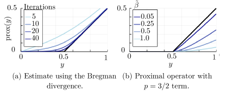
Figure 4.1: Proximal operators for $R(x)=\dfrac{1}{2}\lvert x\rvert$ and some smooth relatives. The black line in both plots is the soft thresholding function, which is the proximal operator for the absolute value function, i.e., $\text{prox}(y)=\operatorname*{argmin}_{x}\dfrac{1}{2}(x-y)^{2}+\dfrac{1}{2}\lvert x\rvert$. (a) As described in [ochs:2016:techniquesgradientbasedbilevel], the number of iterations of the primal-dual algorithm with the Bregman proximity function acts as a smoothing parameter for the proximal operator estimate and the estimate improves as the number of iterations increases (from light to dark lines). (b) Smooth proximal operator for the non-smooth penalty function (4.23) for $p=3/2$, $\beta=0.5$, and four different values of $\tilde{\beta}$. The proximal operator is closer to soft thresholding for smaller values of $\tilde{\beta}$ (darker lines).

christof:2020:gradientbasedsolutionalgorithms shows another approach to achieving a smooth optimization algorithm for a non-smooth cost function. Ref. [christof:2020:gradientbasedsolutionalgorithms] specifically considers cost functions with penalty functions of the form

$$\phi(z)=\beta\lvert z\rvert+2\tilde{\beta}\frac{\lvert z\rvert^{p}}{p}\text{ for }1<p<2.$$ (4.23)

As a simple demonstration, in the case where there are no convolutional filters and $p=3/2$, the lower-level cost function is the proximal operator

$$\mathrm{prox}_{\phi}(y) =\operatorname*{argmin}_{x}\dfrac{1}{2}(x-y)^{2}+\phi(x).$$

Differentiating and solving for the minimizer yields

$$\mathrm{prox}_{\phi}(y) =\begin{cases}\mathrm{sign}(y)\left(\sqrt{\tilde{\beta}^{2}+\lvert y\rvert-\beta}-\tilde{\beta}\right)^{2}&\text{ if }\lvert y\rvert>\beta\\ 0&\mathrm{else,}\end{cases}$$

which is continuous and differentiable everywhere with respect to $y$ despite the non-differential absolute value function in $\phi$! Fig. 4.1 shows this proximal operator alongside the proximal operator when $\phi(z)=\lvert z\rvert$ (soft thresholding). Ref. [christof:2020:gradientbasedsolutionalgorithms] proves that this simple example generalizes to the bilevel problem of learning filters.

4.5 Summary

This section focused on computing $\nabla\ell({\bm{\upgamma}})$, the gradient of the upper-level loss function with respect to the learnable parameters. Section 5 builds on this foundation to consider optimization methods for bilevel problems. Many of those optimization methods can be used in conjunction with the minimizer, translation to a single-level, or unrolled approaches to compute $\nabla\ell({\bm{\upgamma}})$. Thus, how one selects an approach may depend on the structure of the specific bilevel problem, how closely tied one wishes to be to the original bilevel problem, computational cost, and/or gradient accuracy.

The translation to a single-level approach is tailored to a specific type of bilevel problem. A benefit of the translation approach is the ability to use the 1-norm (without any corner rounding) in the lower-level cost function. However, the corresponding drawback is the (current) lack of generality in the minimizer approach; the closed-form expression derived in [sprechmann:2013:supervisedsparseanalysis, mccann:2020:supervisedlearningsparsitypromoting, ghosh:2021:bilevellearningl1regularizers] is specific to using the 1-norm as $\phi$. Expanding this approach to regularizers other than the 1-norm is a possible avenue for future work.

One difference among the methods is whether they depend on the lower-level optimization algorithm; while the unrolled approach depends on the specific optimization algorithm, the minimizer approach and the translation to a single-level approach do not. A resulting downside of unrolling is that one cannot use techniques such as warm starts and non-differentiable restarts, so ${\bm{x}}^{(T)}$ may be farther from the minimizer than the approximation from a similar number of iterations of a more sophisticated, non-differentiable update method. However, the unrolled method’s dependence on $\Psi$ is also a benefit, as an unrolled method can be applied to non-smooth cost functions, as long as the resulting update mapping $\Psi$ is smooth. Further, defining $\Psi$ and the initial starting point ensures that ${\bm{x}}^{(T)}$ is unique, avoiding concerns about non-unique minimizers.

Another advantage of unrolling is that one can run a given number of iterations of the optimization algorithm, without having to reach convergence, and still calculate a valid gradient. Particularly in image reconstruction problems, where finding ${\bm{\hat{x}}}$ exactly can be time intensive, the benefit of a more flexible run-time could outweigh the disadvantages. However, the corresponding downside of unrolling is that the learned hyperparameters are less clearly tied to the original cost function than when one uses the minimizer approach. Section 7.1 further discusses this point in connection to how unrolling for bilevel methods can differ from (deep) learnable optimization algorithms.

One way to connect the minimizer and unrolling strategies is to consider the limit as the number of unrolled iterations approaches infinity. Assuming the optimization algorithm converges, this “fixed point” approach is strongly related to the minimizer approach. For instance, [shaban:2019:truncatedbackpropagationbilevel] shows that backpropagating through the last $\tilde{T}$ iterations of a converged unrolled algorithm can be viewed as approximating the matrix inverse in the minimizer gradient equation (4.8) with an order-$\tilde{T}$ Taylor series. Section 7.2 further discusses how fixed point networks (or “equilibrium networks”) relate the unrolled-to-convergence and minimizer approaches.

Gradient accuracy and computational cost are, unsurprisingly, trade-offs. Tab. 4.1 summarizes the cost of the minimizer and unrolled approaches, derived in Section 4.2.4 and Appendix B respectively, but the total computation will depend on the required gradient accuracy. By accuracy, we mean error from the true bilevel gradient

$$\lVert\underbrace{\hat{\nabla}_{T}\ell({\bm{\upgamma}})}_{\begin{subarray}{c}\text{Estimated}\\ \text{ gradient}\end{subarray}}-\underbrace{\nabla\ell({\bm{\upgamma}})}_{\begin{subarray}{c}\text{True bilevel}\\ \text{gradient}\end{subarray}}\!\!\!\rVert,$$

where $T$ denotes the number of lower-level optimization steps. The unrolled gradient is always accurate for the unrolled mapping, but not for the original bilevel problem. Therefore, unrolling may be more computationally feasible when one cannot run a sufficient number of lower-level optimization steps to reach close enough to a minimizer to assume the gradient in (4.3) is approximately zero [kobler:2021:totaldeepvariation].

	Minimizer	Unrolled: reverse	Unrolled: forward
Memory	0	$\mathcal{O}\!\left(TN\right)$	$\mathcal{O}\!\left(NR\right)$
Hessian-vector products	0	$\mathcal{O}\!\left(T\right)$	$\mathcal{O}\!\left(TR\right)$
Hessian-inverse vector products	1	0	0
Other multiplications	$NR$	$\mathcal{O}\!\left(TNR\right)$	$\mathcal{O}\!\left(NR\right)$

Table 4.1: Memory and computational complexity of the minimizer approach (4.8), reverse-mode unrolled approach (B.2), and forward-mode unrolled approach (B.3) to computing $\nabla_{\bm{\upgamma}}\ell({\bm{\upgamma}}\,;{\bm{\hat{x}}}({\bm{\upgamma}}))$. Computational costs do not include running the optimization algorithm (typically expensive but often comparable across methods), computing $\nabla_{\bm{x}}\ell({\bm{\upgamma}}\,;{\bm{x}}^{(T)})$ (typically cheap), or computing $\nabla_{\bm{\upgamma}}\ell({\bm{\upgamma}}\,;{\bm{x}})$ (frequently zero). Memory requirements do not include storing a single copy of $\bm{x}$, $\bm{A}$, $\bm{\upgamma}$, ${\bm{H}}_{,}$ and ${\bm{J}}$. Recall ${\bm{x}}\in\mathbb{F}^{N}$, ${\bm{\upgamma}}\in\mathbb{F}^{R}$, and there are $T$ iterations of the lower-level optimization algorithm for the unrolled method. Hessian-vector products (first row) and Hessian-inverse-vector products (middle row) are listed separately from all other multiplications (last row) as the computational cost of Hessian operations can vary widely; see discussion in Section 4.2.4.

In all of the approaches considered, the accuracy of the estimated hyperparameter gradient in turn depends on the solution accuracy or number of unrolled iterations of the lower-level cost function. Ref. [mccann:2020:supervisedlearningsparsitypromoting] notes that their translation to a single-level approach failed if they did not optimize the lower-level problem to a sufficient accuracy level. However, [sprechmann:2013:supervisedsparseanalysis, mccann:2020:supervisedlearningsparsitypromoting, ghosh:2021:bilevellearningl1regularizers] did not investigate how the solution accuracy of the lower-level problem impacts the upper-level gradient estimate.

For the minimizer and unrolled approaches, [grazzi:2020:iterationcomplexityhypergradient, ji:2021:bileveloptimizationconvergence] found that the gradient estimate from the minimizer approach converges to the true gradient faster than the unrolled approach (in terms of computation). To state the bounds, [grazzi:2020:iterationcomplexityhypergradient, ji:2021:bileveloptimizationconvergence] assert conditions on the structure of the bilevel problem. They assume that ${\bm{\hat{x}}}({\bm{\upgamma}})$ is the unique minimizer of the lower-level cost function, the Hessian of the lower-level is invertible, the Hessian and Jacobian of $\Upphi$ are Lipschitz continuous with respect to $\bm{x}$, the gradients of the upper-level loss are Lipschitz continuous with respect to $\bm{x}$, the norm of $\bm{x}$ is bounded, and the lower-level cost is strongly convex and Lipschitz smooth for every $\bm{\upgamma}$ value. Section 5.3.1 discusses similar investigations that use these conditions, how easy or hard they are to satisfy, and how they apply to (Ex).

Ref. [grazzi:2020:iterationcomplexityhypergradient] initializes the lower-level iterates for both the unrolled and minimizer approach with the zero vector, i.e., ${\bm{x}}^{(0)}=\bm{0}$. Under their assumptions, [grazzi:2020:iterationcomplexityhypergradient] prove that both the unrolled and minimizer gradients converge linearly in the number of lower-level iterations when the lower-level optimization algorithm and conjugate gradient algorithm for the minimizer approach converge linearly. Although the rate of the approaches is the same, the minimizer approach converges at a faster linear rate and [grazzi:2020:iterationcomplexityhypergradient] generally recommends the minimizer approach, though they found empirically that the unrolled approach may be more reliable when the strong convexity and Lipschitz smooth assumptions on the lower-level cost do not hold.

Ref. [ji:2021:bileveloptimizationconvergence] extended the analysis from [grazzi:2020:iterationcomplexityhypergradient] to consider a warm start initialization for the lower-level optimization algorithm. They similarly find that the minimizer approach has a lower complexity than the unrolled approach. Sections 5.3.2 and 5.3.3 further discuss complexity results after introducing specific bilevel optimization algorithms.

Chapter 5 Gradient-Based Bilevel Optimization Methods

The previous section discussed different approaches to finding $\nabla\ell({\bm{\upgamma}})$, the gradient of the upper-level loss function with respect to the learnable parameters. Building on those results, we now consider approaches for optimizing the bilevel problem. In particular, this section concentrates on gradient-based algorithms for optimizing the hyperparameters. While there is some overlap with single-level optimization methods, this section focuses on the challenges due to the bilevel structure. Therefore, we do not discuss the lower-level optimization algorithms in detail; for overviews of lower-level optimization, see, e.g., [palomar:11:coi, chambolle:2016:introductioncontinuousoptimization].

Gradient-based methods for bilevel problems are an alternative to the approaches described in Section 3, e.g., grid or random search, Bayesian optimization, and trust region methods. By incorporating gradient information, the methods presented in this section can scale to problems having many hyperparameters. In fact, Section 5.3 reviews papers that provide bounds on the number of upper-level gradient descent iterations required to reach a point within some user-defined tolerance of a solution. While the bounds depend on the regularity of the upper-level loss and lower-level cost functions, they do not depend on the number of hyperparameters nor the signal dimension. Although having more hyperparameters will increase computation per iteration, using a gradient descent approach means the number of iterations need not scale with the number of hyperparameters, $R$.

Bilevel gradient methods fall into two broad categories. Most gradient-based approaches to the bilevel problem fall under the first category: double-loop algorithms. These methods involve (i) optimizing the lower-level cost, either to some convergence tolerance if using a minimizer approach or for a certain number of iterations if using an unrolled approach, (ii) calculating $\nabla\ell({\bm{\upgamma}})$, (iii) taking a gradient step in $\bm{\upgamma}$, and (iv) iterating. The first step is itself an optimization algorithm and may involve many inner iterations, thus the categorization as a “double-loop algorithm.”

The second category, “single-loop” algorithms, involve one loop, with each iteration containing one gradient step for both the lower-level optimization variable, $\bm{x}$, and the upper-level optimization variable, $\bm{\upgamma}$. Single-loop algorithms may alternate updates or update the variables simultaneously. Section 4 used $t$ to denote the lower-level iteration counter; this section introduces $u$ as the iteration counter for the upper-level iterations and as the single iteration counter for single-loop algorithms.

5.1 Double-Loop Algorithms

After using one of the approaches in Section 4 to compute the hyperparameter gradient $\nabla\ell({\bm{\upgamma}})$, typical double-loop algorithms for bilevel problems run some type of gradient descent on the upper-level loss. Alg. 1 shows an example double-loop algorithm [pedregosa:2016:hyperparameteroptimizationapproximate]. Line 11 of Alg. 1 uses the CG method to compute the product of the Hessian inverse with a vector in (4.8). Thus, Alg. 1 actually involves three loops. However, the third, CG loop is often left as an implementation detail and we will continue to use the term “double-loop” for the overall strategy. There is similarly a third, hidden loop in approaches that use the reverse mode method for backpropogation in the unrolled approaches described in Section 4.4.

The final iterate of a lower-level optimizer is only an approximation of the lower-level minimizer. However, the minimizer approach to calculating the upper-level gradient $\nabla\ell({\bm{\upgamma}})$ from Section 4.2 assumes $\nabla_{\bm{x}}\Upphi({\bm{\hat{x}}}\,;{\bm{\upgamma}})=\bm{0}$. Any error stemming from not being at an exact critical point can be magnified in the full calculation (4.8), and the resulting hyperparameter gradient will be an approximation of the true gradient, as illustrated in Fig. 5.1. Thus, how accurately one optimizes the lower-level problem can greatly impact the quality of the learned parameters, $\hat{{\bm{\upgamma}}}$ [chen:2013:revisitinglossspecifictraining]. Alternatively, if one uses the unrolled approach with a set number of iterations (4.17), the gradient is accurate for that specific number of iterations, but the lower-level optimization sequence may not have converged and the overall method may not accurately approximate the original bilevel problem.

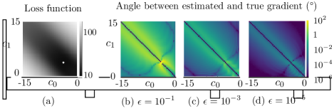
Figure 5.1: Error in the upper-level gradient, $\nabla\ell({\bm{\upgamma}})$, for various convergence thresholds for the lower-level optimizer. The bilevel problem is (Ex) with a single filter, ${\bm{c}}=\begin{bmatrix}c_{0}&c_{1}\end{bmatrix}$, $e^{\beta_{0}}=0$, $e^{\beta_{1}}=-5$, and $\phi(z)=z^{2}$ so there is an analytic solution for $\nabla\ell({\bm{\upgamma}})$. The training data is piece-wise constant 1d signals and the learnable hyperparameters are the filter coefficients. (a) Upper-level loss function, $\ell({\bm{\upgamma}})$. The cost function is low (dark) where $c_{1}\approx c_{0}$, corresponding to approximate finite differences. The star indicates the minimum. (b-d) Error in the estimated gradient angle using the minimizer approach (4.8), defined as the angle between $\hat{\nabla}\ell({\bm{\upgamma}})$ and $\nabla\ell({\bm{\upgamma}})$, when the lower-level optimization is run until $\left\lVert\nabla_{\bm{x}}\Upphi({\bm{x}}\,;{\bm{\upgamma}})\right\rVert_{2}<\epsilon$.

Due to such inevitable inexactness when computing $\nabla\ell({\bm{\upgamma}})$, one may wonder about the convergence of double-loop algorithms for bilevel problems. Considering the unrolled method of computing $\nabla\ell({\bm{\upgamma}})$, [franceschi:2018:bilevelprogramminghyperparameter] showed that the sequence of hyperparameter values in a double-loop algorithm, ${\bm{\upgamma}}^{(u)}$, converges as the number of unrolled iterations increases. To prove this result, [franceschi:2018:bilevelprogramminghyperparameter] assumed the hyperparameters were constrained to a compact set, $\ell({\bm{\upgamma}}\,;\,{\bm{x}})$ and $\Upphi({\bm{x}}\,;{\bm{\upgamma}})$ are jointly continuous, there is a unique solution ${\bm{\hat{x}}}({\bm{\upgamma}})$ to the lower-level cost for all $\bm{\upgamma}$; and ${\bm{\hat{x}}}({\bm{\upgamma}})$ is bounded for all $\bm{\upgamma}$. These conditions are satisfied for problems with strictly convex lower-level cost functions and suitable box constraints on $\bm{\upgamma}$. Section 5.3.2 further discusses convergence results for double-loop algorithms.

Algorithm 1: Hyperparameter optimization with approximate gradient (HOAG) from [pedregosa:2016:hyperparameteroptimizationapproximate]. As written below, the HOAG algorithm is impractical because it uses ${\bm{\hat{x}}}({{\bm{\upgamma}}^{(u)}})$ in the convergence criteria; however, for strongly convex lower-level problems, the convergence criteria, $\|{\bm{\hat{x}}}({{\bm{\upgamma}}^{(u)}})-{{\bm{x}}^{(t)}}({{\bm{\upgamma}}^{(u)}})\|$, is easily upper-bounded.

1:procedure HOAG($\{{\epsilon^{(u)}},u=1,2,\ldots\}$, ${\bm{\upgamma}}^{(0)}$, ${\bm{x}}^{(0)}$, $\bm{y}$)

2:     for $u$ do=0,1,…$\triangleright$ Upper-level iteration counter

3:         $t=0$ $\triangleright$ Lower-level iteration counter

4:         while $\|{\bm{\hat{x}}}({{\bm{\upgamma}}^{(u)}})-{{\bm{x}}^{(t)}}({{\bm{\upgamma}}^{(u)}})\|\geq{\epsilon^{(u)}}$ do

5:              ${{\bm{x}}^{(t+1)}}=\Psi({{\bm{x}}^{(t)}}\,;{{\bm{\upgamma}}^{(u)}})$ $\triangleright$ Lower-level optimization step

6:              $t=t+1$

7:         end while

8:         Compute gradient $\nabla_{\bm{x}}\ell({{\bm{\upgamma}}^{(u)}}\,;{\bm{x}}^{(t)})$ and

9:         Jacobian $\nabla_{{\bm{x}}{\bm{\upgamma}}}\Upphi({{\bm{x}}^{(t)}}\,;{{\bm{\upgamma}}^{(u)}})$

10:         Using CG, find $\bm{q}$ such that

11:$\quad\quad\quad\|\nabla_{{\bm{x}}{\bm{x}}}\Upphi({{\bm{x}}^{(t)}}\,;{{\bm{\upgamma}}^{(u)}}){\bm{q}}-\nabla_{\bm{x}}\ell({{\bm{\upgamma}}^{(u)}}\,;{\bm{x}}^{(t)})\|\leq{\epsilon^{(u)}}$

12:         ${\bm{g}}=\nabla_{\bm{\upgamma}}\ell({{\bm{\upgamma}}^{(u)}}\,;{{\bm{x}}^{(t)}})-\left(\nabla_{{\bm{x}}{\bm{\upgamma}}}\Upphi({{\bm{x}}^{(t)}}\,;{{\bm{\upgamma}}^{(u)}})\right)^{\prime}{\bm{q}}$ $\triangleright$ From (4.8)

13:         ${{\bm{\upgamma}}^{(u+1)}}={{\bm{\upgamma}}^{(u)}}-\frac{1}{L}{\bm{g}}$ $\triangleright$ $L$ is a Lipschitz constant of $\nabla\ell({\bm{\upgamma}})$

14:     end for

15:     return ${{\bm{\upgamma}}^{(u+1)}}$

16:end procedure

pedregosa:2016:hyperparameteroptimizationapproximate proved a similar result for the minimizer formula (4.8) using CG to compute (4.10). Specifically, [pedregosa:2016:hyperparameteroptimizationapproximate] showed that the hyperparameter sequence convergences to a stationary point if the sequence of positive tolerances, $\{{\epsilon^{(u)}},u=1,2,\ldots\}$ in Alg. 1, is summable. The convergence results are for the algorithm version shown in Alg. 1 that uses a Lipschitz constant of $\ell({\bm{\upgamma}})$, which is generally unknown. Although [pedregosa:2016:hyperparameteroptimizationapproximate] discusses various empirical strategies for setting the step size, the convergence theory does not consider those variations. Thus, the double-loop algorithm [pedregosa:2016:hyperparameteroptimizationapproximate] requires multiple design decisions.

There are four key design decisions for double-loop algorithms:

1. How accurately should one solve the lower-level problem?

2. What upper-level gradient descent algorithm should one use?

3. How does one pick the step size for the upper-level descent step?

4. What stopping criteria should one use for the upper-level iterations?

This section first reviews some (largely heuristic) approaches to these design decisions and presents example bilevel gradient descent methods with no (or few) assumptions beyond those made in Section 4. Without any further assumptions, the answers to the questions above are based on heuristics, with few theoretical guarantees but often providing good experimental results. Section 5.3.2 discusses recent methods with stricter assumptions on the bilevel problem and their theory-backed answers to the above questions.

The first step in a double-loop algorithm is to optimize the lower-level cost, for which there are many optimization approaches. The only restriction is computability of the gradient of the upper-level loss $\nabla\ell({\bm{\upgamma}})$, which typically includes a smoothness assumption (see Section 4 for discussion). Many bilevel methods use a standard optimizer for the lower-level problem, although others propose new variants, e.g., [chen:2021:learnabledescentalgorithm].

The first design decision (how accurately to solve the lower-level problem) involves a trade-off between computational complexity and accuracy. Example convergence criteria are fairly standard to the optimization literature, e.g., the Euclidean norm of the lower-level gradient [hintermuller:2020:dualizationautomaticdistributed, chen:2014:insightsanalysisoperator] or the normalized change in the estimate $\bm{x}$ [sixou:2020:adaptativeregularizationparameter] being less than some threshold. For example, [chen:2014:insightsanalysisoperator] used a convergence criteria of $\|\nabla_{\bm{x}}\Upphi({{\bm{x}}^{(t)}}\,;{\bm{\upgamma}})\|_{2}\leq 10^{\text{-}3}$ (where the image scale is 0-255). As mentioned above, [pedregosa:2016:hyperparameteroptimizationapproximate] uses a sequence of convergence tolerances so that the lower-level cost function is optimized more accurately as the upper-level iterations continue.

Ref. [chen:2013:revisitinglossspecifictraining] investigated the importance of lower-level optimization accuracy. The authors use the same training model as in [samuel:2009:learningoptimizedmap], which is the bilevel extension of the Field of Experts [roth:2005:fieldsexpertsframework], but varied the convergence criteria for the lower-level problem. When using a convergence tolerance of $\|\nabla_{\bm{x}}\Upphi({{\bm{x}}^{(t)}}\,;{\bm{\upgamma}})\|_{2}/\sqrt{N}\leq 10^{\text{-}5}$, [chen:2013:revisitinglossspecifictraining] found an average improvement of 0.65dB in the PSNR for test images over [samuel:2009:learningoptimizedmap], who ran their lower-level optimization algorithm for a set number of iterations. Ref. [chen:2013:revisitinglossspecifictraining] also plots the test PSNR and training loss versus the lower-level convergence criteria and shows how test PSNR increases and training loss decreases with increased lower-level solution accuracy for this specific filter learning bilevel problem.

Many publications do not report a specific threshold or discuss how they chose a convergence criteria or number of lower-level iterations. However, a few note the importance of such decisions. For example, [mccann:2020:supervisedlearningsparsitypromoting] found that their learning method fails if the lower-level optimizer is insufficiently close to the minimizer and [chen:2014:insightsanalysisoperator] stated their results are “significantly better” than [samuel:2009:learningoptimizedmap] because they solve the lower-level problem “with high[er] accuracy.”

After selecting a level of accuracy, finding (an approximation of) ${\bm{\hat{x}}}$, and calculating $\nabla\ell({\bm{\upgamma}})$ using one of the approaches from Section 4, one must make the second design decision: which gradient-based method to use for the upper-level problem. Many bilevel methods suggest a simple gradient-based method such as plain gradient descent (GD) [peyre:2011:learninganalysissparsity], GD with a line search (see the third design decision), projected GD [antil:2020:bileveloptimizationdeep], or stochastic GD [mccann:2020:supervisedlearningsparsitypromoting]. These methods update $\bm{\upgamma}$ based on only the current upper-level gradient; they do not have memory of previous gradients nor require/estimate any second-order information.

Methods that incorporate some second-order information use more memory and computation per iteration, but may converge faster than basic GD methods. For example, Broyden-Fletcher-Goldfarb-Shanno (BFGS) and L-BFGS (the low-memory version of BFGS) [byrd:95:alm] are quasi-Newton algorithms that store and update an approximate Hessian matrix that serves as a preconditioner for the gradient. The $R\times R$ size of the Hessian grows as the number hyperparameters increases, but quasi-Newton methods like L-BFGS use practical rank-1 updates with storage $\mathcal{O}\!\left(R\right)$. Adam [kingma:2015:adammethodstochastic] is a popular GD method, especially in the machine learning community, that tailors the step size (equivalently the learning rate) for each hyperparameter based on moments of the gradient. Although Adam requires its own parameters, the parameters are relatively easy to set and the default settings often perform adequately. Example bilevel papers using methods with second-order information include those that use BFGS [holler:2018:bilevelapproachparameter], L-BFGS [chen:2014:insightsanalysisoperator], Gauss-Newton [fehrenbach:2015:bilevelimagedenoising], and Adam [chen:2021:learnabledescentalgorithm].

Many gradient-based methods require selecting a step size parameter, e.g., one must choose a step size $\alpha_{\ell}$ in classical GD:

$${\bm{\upgamma}}^{(u+1)}={\bm{\upgamma}}^{(u)}-\alpha_{\ell}\,{\nabla\ell\left({\bm{\upgamma}}^{(u)}\right)}.$$

This choice is the third design decision. Bilevel problems are generally non-convex, and typically a Lipschitz constant is unavailable, so line search strategies initially appear appealing. However, any line search strategy that involves attempting multiple values quickly becomes computationally intractable for large-scale problems. The upper-level loss function in bilevel problems is particularly expensive to evaluate because it requires optimizing the lower-level cost! Further, recall that the upper-level loss is typically an expectation over multiple training samples (UL), so evaluating a single step size involves optimizing the lower-level cost $J$ times (or using a stochastic approach and selecting a batch size).

Despite these challenges, a line search strategy may be viable if it rarely requires multiple attempts. For example, the backtracking line search in [hintermuller:2020:dualizationautomaticdistributed] that used the Armijo–Goldstein condition required 57-59 lower-level evaluations (per training example) over 40 upper-level gradient descent steps, so most upper-level steps required only one lower-level evaluation. Other bilevel papers that used backtracking with Armijo-type conditions include [holler:2018:bilevelapproachparameter, sixou:2020:adaptativeregularizationparameter, calatroni:2017:bilevelapproacheslearning]; [lecouat:2020:flexibleframeworkdesigning] used the Barzilai-Borwein method for picking an adaptive step size.

Other approaches to determining the step size are: (i) normalize the gradient by the dimension of the data and pick a fixed step size [mccann:2020:supervisedlearningsparsitypromoting], (ii) pick a value that is small enough based on experience [peyre:2011:learninganalysissparsity], or (iii) adapt the step size based on the decrease from the previous iteration [pedregosa:2016:hyperparameteroptimizationapproximate].

The fourth design decision is the convergence criteria for the upper-level loss. As with the lower-level convergence criteria, few publications include a specific threshold, but most bilevel methods tend to use traditional convergence criteria such as the norm of the hyperparameter gradient falling below some threshold [holler:2018:bilevelapproachparameter], the norm of the change in parameters falling below some threshold [chen:2014:insightsanalysisoperator], and/or reaching a maximum iteration count (many papers). One specific example is to terminate when the normalized change in learned parameters, $\|{{\bm{\upgamma}}^{(u+1)}}-{{\bm{\upgamma}}^{(u)}}\|/\|{{\bm{\upgamma}}^{(u)}}\|,$ is below 0.01 [sixou:2020:adaptativeregularizationparameter]. The normalized change bound is convenient because it is unitless and thus invariant to scaling of $\bm{\upgamma}$.

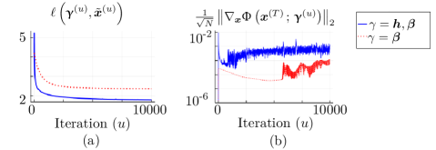
Figure 5.2: Example convergence plots for a double-loop bilevel method when $\bm{\upgamma}$ includes $\bm{h}$ and $\bm{\beta}$ (solid lines) and when ${\bm{\upgamma}}={\bm{\beta}}$ (dotted lines). (a) Estimated upper-level loss function evaluated at the current estimate of the lower-level minimizer, ${\bm{x}}^{(T)}={\bm{x}}^{(T)}({\bm{\upgamma}}^{(u)})$, versus upper-level iteration $u$. (b) Lower-level convergence metric, averaged over all training samples, versus upper-level iteration. The estimated lower-level minimizer remains close to convergence throughout the double-loop method.

Fig. 5.2 shows example upper-level convergence plots for a double-loop algorithm for the bilevel problem (Ex). After an initial first run of OGM to get the lower-level initialization ${\bm{\hat{x}}}({\bm{\upgamma}}^{(0)})$ such that $\tfrac{1}{\sqrt{N}}\left\lVert\nabla_{\bm{x}}\Upphi\left({\bm{\hat{x}}}({\bm{\upgamma}}^{(0)})\,;\,{\bm{\upgamma}}^{(0)}\right)\right\rVert_{2}<10^{\text{-}7}$, the lower-level optimizer consisted of 10 iterations of OGM [kim:18:aro], initialized with the estimate from the previous upper-level iteration. The upper-level optimizer is Adam [kingma:2015:adammethodstochastic] with the default parameters, negating the need for a separate upper-level step-size parameter. We ran 10,000 outer-loop iterations. The final norm of the upper-level gradient, $\tfrac{1}{\sqrt{R}}\|\nabla({\bm{\upgamma}}^{(U)})\|$ was 0.08 when learning the filter coefficients and tuning parameters and $5\cdot 10^{\text{-}4}$ when learning only $\bm{\beta}$. Fig. 6.2 shows the corresponding denoised images and Appendix D.2 further details the experiment settings.

5.2 Single-Loop Algorithms

Unlike double-loop algorithms, single-loop algorithms take a gradient step in $\bm{\upgamma}$ without optimizing the lower-level problem each step. Two early bilevel method papers [haber:2003:learningregularizationfunctionals, kunisch:2013:bileveloptimizationapproach] proposed single-loop approaches based on solving the system of equations that arises from the Lagrangian.

The system of equations approach in [haber:2003:learningregularizationfunctionals, kunisch:2013:bileveloptimizationapproach] closely follows the KKT perspective on the minimizer approach in Section 4.2.2. Recall that the gradient of the lower-level problem is zero at a minimizer, ${\bm{\hat{x}}}$, and one can use this equality as a constraint on the upper-level loss function. The corresponding Lagrangian is

$$L({\bm{x}},{\bm{\upgamma}},{\bm{\nu}}) =\ell({\bm{\upgamma}}\,;{\bm{x}})+{\bm{\nu}}^{\prime}\nabla_{\bm{x}}\Upphi({\bm{x}}\,;{\bm{\upgamma}}),$$ (5.1)

where $\bm{\nu}$ is a vector of Lagrange multipliers. For the filter learning example (Ex), the Lagrangian is

$$L({\bm{x}},{\bm{\upgamma}},{\bm{\nu}}) =\dfrac{1}{2}\|{\bm{x}}-{\bm{x}}^{\text{true}}\|^{2}_{2}+$$

$$\,\,{\bm{\nu}}^{\prime}\left({\bm{A}}^{\prime}({\bm{A}}{\bm{x}}-{\bm{y}})+e^{\beta_{0}}\sum_{k=1}^{K}e^{\beta_{k}}\tilde{{\bm{c}}}_{k}\circledast\phi.({\bm{c}}_{k}\circledast{\bm{x}};\epsilon)\right).$$

As in Section 4.2.2, we consider derivatives of the Lagrangian with respect to $\bm{\nu}$, $\bm{x}$, and $\bm{\upgamma}$. Here are the general expressions and the specific equations for the filter learning example (Ex) when considering the element of $\bm{\upgamma}$ corresponding to $\beta_{k}$:

$$\nabla_{\bm{\nu}}L({\bm{x}},{\bm{\upgamma}},{\bm{\nu}}) =\nabla_{\bm{x}}\Upphi({\bm{x}}\,;{\bm{\upgamma}})$$

$$={\bm{A}}^{\prime}({\bm{A}}{\bm{x}}-{\bm{y}})+e^{\beta_{0}}\sum_{k=1}^{K}e^{\beta_{k}}\tilde{{\bm{c}}}_{k}\circledast\phi.({\bm{c}}_{k}\circledast{\bm{x}};\epsilon)$$

$$\nabla_{\bm{x}}L({\bm{x}},{\bm{\upgamma}},{\bm{\nu}}) =\nabla_{\bm{x}}\ell({\bm{\upgamma}}\,;{\bm{x}})+\nabla_{{\bm{x}}{\bm{x}}}\Upphi({\bm{x}}\,;{\bm{\upgamma}}){\bm{\nu}}$$

$$={\bm{x}}-{\bm{x}}^{\text{true}}+{\bm{A}}^{\prime}{\bm{A}}{\bm{\nu}}+e^{\beta_{0}}\sum_{k}e^{\beta_{k}}{\bm{C}}_{k}^{\prime}\text{diag}({\ddot{\phi}}.({\bm{c}}_{k}\circledast{\bm{\hat{x}}})){\bm{C}}_{k}{\bm{\nu}}$$

$$\nabla_{\bm{\upgamma}}L({\bm{x}},{\bm{\upgamma}},{\bm{\nu}}) =\nabla_{\bm{\upgamma}}\ell({\bm{\upgamma}}\,;\,{\bm{x}})+{\bm{\nu}}^{\prime}\nabla_{{\bm{x}}{\bm{\upgamma}}}\Upphi({\bm{x}}\,;{\bm{\upgamma}})$$

$$={\bm{\nu}}^{\prime}\left(e^{\beta_{0}}e^{\beta_{k}}\tilde{{\bm{c}}}_{k}\circledast{{\dot{\phi}}}.({\bm{c}}_{k}\circledast{\bm{\hat{x}}})\right)\text{ when }{\bm{\upgamma}}=\beta_{k}.$$

These expressions are equivalent to the primal, adjoint, and optimality conditions respectively in [kunisch:2013:bileveloptimizationapproach].

Here the minimizer and single-loop approach diverge. Section 4.2.2 used the above Lagrangian gradients to solve for $\hat{{\bm{\nu}}}$, substitute $\hat{{\bm{\nu}}}$ into the gradient of the Lagrangian with respect to $\bm{\upgamma}$, and thus find the minimizer expression for $\nabla\ell({\bm{\upgamma}})$. The single-loop approach instead considers solving the system of gradient equations directly:

$${\bm{G}}({\bm{x}},{\bm{\upgamma}},{\bm{\nu}})=\begin{bmatrix}\nabla_{\bm{\nu}}L({\bm{x}},{\bm{\upgamma}},{\bm{\nu}})\\ \nabla_{\bm{x}}L({\bm{x}},{\bm{\upgamma}},{\bm{\nu}})\\ \nabla_{\bm{\upgamma}}L({\bm{x}},{\bm{\upgamma}},{\bm{\nu}})\end{bmatrix}=\bm{0}.$$

For example, [kunisch:2013:bileveloptimizationapproach] proposed a Newton algorithm using the Jacobian of the gradient matrix $\bm{G}$.

Another approach to single-loop algorithms is to replace the “while” loop in Alg. 1 line 4 with a single gradient step in the lower-level optimization variables. Two single-loop algorithms are the two-timescale stochastic approximation (TTSA) method [hong:2020:twotimescaleframeworkbilevel] and the Single Timescale stochAstic BiLevEl optimization (STABLE) method [chen:2021:singletimescalestochasticbilevel]. Alg. 2 shows TTSA as an example single-loop algorithm. Both TTSA and STABLE alternate between one gradient step for the lower-level cost and one gradient step for the upper-level problem.

There are two main challenges in designing such a single loop algorithm for bilevel optimization. Because both TTSA and STABLE use the minimizer approach (4.8) to finding the upper-level gradient, the first challenge is ensuring the current lower-level iterate is close enough to the minimizer to calculate a useful upper-level gradient. TTSA addresses this challenge by taking larger steps for the lower-level problem while STABLE addresses this using a lower-level update that better predicts the next lower-level minimizer, ${\bm{\hat{x}}}({{\bm{\upgamma}}^{(u+1)}})$.

The second main challenge is estimating the upper-level gradient, even given stochastic estimates of $\nabla_{{\bm{x}}{\bm{x}}}\Upphi$ and $\nabla_{{\bm{x}}{\bm{\upgamma}}}\Upphi$, because the minimizer equation (4.8) is nonlinear. The theoretical results about TTSA are built on the assumption that the upper-level gradient is biased due to this nonlinearity. In contrast, STABLE uses recursion to update estimates of the gradients and thus reduce variance. Section 5.3.3 goes into more detail about both algorithms.

Algorithm 2: Two-Timescale Stochastic Approximation (TTSA) method from [hong:2020:twotimescaleframeworkbilevel]. TTSA includes a possible projection of the hyperparameter after each gradient step onto a constraint set, not shown here. The tildes denote stochastic approximations for the corresponding expressions.

1:procedure TTSA(${\bm{\upgamma}}^{(0)}$, ${\bm{x}}^{(0)}$, ${\alpha_{\ell}^{(u)}}$, ${\alpha_{\Upphi}^{(u)}}$)

2:     for $u=1,\ldots$ do

3:         ${{\bm{x}}^{(u+1)}}={{\bm{x}}^{(u)}}-{\alpha_{\Upphi}^{(u)}}\tilde{\nabla}_{\bm{x}}\Upphi({{\bm{x}}^{(u)}};{{\bm{\upgamma}}^{(u)}})$

4:         ${\bm{g}}=\nabla_{\bm{\upgamma}}{\ell^{(u)}}-\left(\tilde{\nabla}_{{\bm{x}}{\bm{\upgamma}}}{\Upphi^{(u)}}\right)^{\prime}\left(\tilde{\nabla}_{{\bm{x}}{\bm{x}}}{\Upphi^{(u)}}\right)^{\text{-}1}\nabla_{\bm{x}}{\ell^{(u)}}$

5:         ${{\bm{\upgamma}}^{(u+1)}}={{\bm{\upgamma}}^{(u)}}-{\alpha_{\ell}^{(u)}}{\bm{g}}$

6:     end for

7:end procedure

5.3 Complexity Analysis

A series of recent papers established finite-time sample complexity bounds for stochastic bilevel optimization methods based on gradient descent for the upper-level loss and lower-level cost. Ref.s [ghadimi:2018:approximationmethodsbilevel, ji:2021:bileveloptimizationconvergence] use double-loop approaches and [hong:2020:twotimescaleframeworkbilevel, chen:2021:singletimescalestochasticbilevel] use single-loop algorithms. Unlike most of the methods discussed in Section 5.1, these papers make additional assumptions about the upper and lower-level functions then select the upper and lower-level step sizes to ensure convergence.

In these works, “finite-time sample complexity” refers to big-O bounds on a number of iterations that ensures one reaches a minimizer to within some desired tolerance. In contrast to asymptotic convergence analysis, finite-time bounds provide information about the estimated hyperparameters, ${\bm{\upgamma}}^{(u)}$, after a finite number of upper-level iterations. These bounds depend on problem-specific quantities, such as Lipschitz constants, but not on the hyperparameter or signal dimensions.

To summarize the results, this section returns to the notation from the introduction where the upper-level loss may be deterministic or stochastic, e.g., the bilevel problem is

$$\hat{{\bm{\upgamma}}} =\operatorname*{argmin}_{\bm{\upgamma}}\ell({\bm{\upgamma}})\text{ with }\ell({\bm{\upgamma}})=\begin{cases}\ell({\bm{\upgamma}},{\bm{\hat{x}}}({\bm{\upgamma}}))&\text{deterministic}\\ \mathbb{E}\left[\ell({\bm{\upgamma}},{\bm{\hat{x}}}({\bm{\upgamma}}))\right]&\text{ stochastic. }\end{cases}$$ (5.2)

The expectation in (5.2) can have different meanings depending on the setting. When one has $J$ training images with one noise realization per image, one often picks a random subset (“minibatch”) of those $J$ images for each update of $\bm{\upgamma}$, corresponding to stochastic gradient descent of the upper-level loss. In this setting, the randomness is a property of the algorithm, not of the upper-level loss, and the expectation reduces to the deterministic case. Section 7.5 discusses other possible definitions of the stochastic bilevel formulation.

The complexity results (summarized in Tab. 5.1) are all in terms of finding ${\bm{\upgamma}}_{\epsilon}$, defined as an $\epsilon$-optimal solution. In the (atypical) setting where $\ell({\bm{\upgamma}})$ is convex, ${\bm{\upgamma}}_{\epsilon}$ is an $\epsilon$-optimal solution if it satisfies either $\ell({\bm{\upgamma}}_{\epsilon})-\ell(\hat{{\bm{\upgamma}}})\leq\epsilon$ [ghadimi:2018:approximationmethodsbilevel, ji:2021:bileveloptimizationconvergence, hong:2020:twotimescaleframeworkbilevel] or $\left\lVert\hat{{\bm{\upgamma}}}-{\bm{\upgamma}}_{\epsilon}\right\rVert^{2}\leq\epsilon$ [chen:2021:singletimescalestochasticbilevel]. (These conditions are equivalent if $\ell$ is strongly convex in $\bm{\upgamma}$, but can differ otherwise.) In the (common) non-convex setting, ${\bm{\upgamma}}_{\epsilon}$ is typically called an $\epsilon$-stationary point if it satisfies $\left\lVert\nabla\ell({\bm{\upgamma}}_{\epsilon})\right\rVert^{2}\leq\epsilon$ [ghadimi:2018:approximationmethodsbilevel, ji:2021:bileveloptimizationconvergence, chen:2021:singletimescalestochasticbilevel]. In the stochastic setting, ${\bm{\upgamma}}_{\epsilon}$ must satisfy these conditions in expectation.

		Upper-level gradients	Lower-level gradients
Double- loop	BA	$\mathcal{O}\!\left(\text{log}\left(\frac{1}{\epsilon^{2}}\right)\right)$	$\mathcal{O}\!\left(\text{log}\left(\frac{1}{\epsilon^{3}}\right)\right)$
	stocBiO	$\mathcal{O}\!\left(\frac{1}{\epsilon^{2}}\right)$	$\mathcal{O}\!\left(\frac{1}{\epsilon^{2}}\right)$
Single- loop	TTSA	$\mathcal{O}\!\left(\frac{1}{\epsilon^{2.5}}\right)$	$\mathcal{O}\!\left(\frac{1}{\epsilon^{2.5}}\right)$
	STABLE	$\mathcal{O}\!\left(\frac{1}{\epsilon^{2}}\right)$	$\mathcal{O}\!\left(\frac{1}{\epsilon^{2}}\right)$

Table 5.1: Finite-time sample complexities for the stochastic bilevel problem in the common scenario where $\ell$ is non-convex when using BA [ghadimi:2018:approximationmethodsbilevel], stocBiO [ji:2021:bileveloptimizationconvergence], TTSA [hong:2020:twotimescaleframeworkbilevel], and STABLE [chen:2021:singletimescalestochasticbilevel]. When $\ell$ is strongly convex, the sample complexity of STABLE is $\mathcal{O}\!\left(\frac{1}{\epsilon^{1}}\right)$ (for the upper- and lower-level gradients), which is the same as single level stochastic gradient algorithms. See cited papers for other complexity results when $\ell$ is strongly convex.

The following sections briefly describe the BA, stocBiO, TTSA, and STABLE algorithms. The literature in this area is quickly evolving; between the writing and editing of this work, new double-loop and single-loop methods appeared with improved complexity results. For example, [yang:2021:provablyfasteralgorithms, khanduri:2021:nearoptimalalgorithmstochastic] concurrently proposed bilevel optimization methods that leverage momentum and variance reduction techniques to reduce the bound on the number of iterations to $\widetilde{\mathcal{O}}\!\left(\frac{1}{\epsilon^{1.5}}\right)$ for both upper-level and lower-level gradients. Ref. [yang:2021:provablyfasteralgorithms] achieved this complexity result for both a double-loop method and a single-loop method.

Whether double-loop or single-loop methods are preferred is an open question. Refs. [ji:2021:bileveloptimizationconvergence, yang:2021:provablyfasteralgorithms] find that double-loop methods converge faster (in terms of wall time) than single-loop methods. The authors hypothesize that $\nabla\ell({\bm{\upgamma}})$ is sensitive enough to changes in the estimate of the lower-level optimizer that the increased accuracy of the double-loop estimates of $\nabla\ell({\bm{\upgamma}})$ is worth the additional lower-level optimization time. Future work should test this hypothesis in different experimental settings and establish guidelines on when to use a double-loop or single-loop algorithm.

5.3.1 Assumptions

References [ghadimi:2018:approximationmethodsbilevel, ji:2021:bileveloptimizationconvergence, hong:2020:twotimescaleframeworkbilevel, chen:2021:singletimescalestochasticbilevel] all make similar assumptions about $\ell$ and $\Upphi$ to derive theoretical results for their proposed bilevel optimization methods. We first summarize the set of sufficient conditions from [ghadimi:2018:approximationmethodsbilevel], and later note any additional assumptions used by the other methods. The conditions in [ghadimi:2018:approximationmethodsbilevel] on the upper-level function, $\ell({\bm{\upgamma}}\,;\,{\bm{x}})$, are:

1. $\forall{\bm{\upgamma}}\in\mathbb{F}^{R}$, $\nabla_{\bm{\upgamma}}\ell({\bm{\upgamma}},{\bm{x}})$ and $\nabla_{\bm{x}}\ell({\bm{\upgamma}},{\bm{x}})$ are Lipschitz continuous with respect to $\bm{x}$, with corresponding Lipschitz constants $L_{{\bm{x}},\nabla_{\bm{\upgamma}}\ell}$ and $L_{{\bm{x}},\nabla_{\bm{x}}\ell}$. (These constants are independent of $\bm{x}$ and $\bm{\upgamma}$.)

2. The gradient with respect to $\bm{x}$ is bounded, i.e.,
   $\left\lVert\nabla_{\bm{x}}\ell({\bm{\upgamma}},{\bm{x}})\right\rVert\leq C_{\nabla_{\bm{x}}\ell},\ \forall{\bm{x}}\in\mathbb{F}^{N}$.

3. $\forall{\bm{x}}\in\mathbb{F}^{N}$, $\nabla_{\bm{x}}\ell({\bm{\upgamma}},{\bm{x}})$ is Lipschitz continuous with respect to $\bm{\upgamma}$, with corresponding Lipschitz constant $L_{{\bm{\upgamma}},\nabla_{\bm{x}}\ell}$.

The conditions in [ghadimi:2018:approximationmethodsbilevel] on the lower-level function, $\Upphi({\bm{x}}\,;{\bm{\upgamma}})$, are:

1. $\Upphi$ is continuously twice differentiable in $\bm{\upgamma}$ and $\bm{x}$.

2. $\forall{\bm{\upgamma}}\in\mathbb{F}^{R}$, $\nabla_{\bm{x}}\Upphi({\bm{x}}\,;{\bm{\upgamma}})$ is Lipschitz continuous with respect to $\bm{x}$ with corresponding constant $L_{{\bm{x}},\nabla_{\bm{x}}\Upphi}$.

3. $\forall{\bm{\upgamma}}\in\mathbb{F}^{R}$, $\Upphi({\bm{x}}\,;{\bm{\upgamma}})$ is strongly convex with respect to $\bm{x}$, i.e., $\mu_{{\bm{x}},\Upphi}\bm{I}\preceq\nabla_{\bm{x}}^{2}\Upphi({\bm{\upgamma}}\,;{\bm{x}})$, for some $\mu_{{\bm{x}},\Upphi}>0$.

4. $\forall{\bm{\upgamma}}\in\mathbb{F}^{R}$, $\nabla_{{\bm{x}}{\bm{x}}}\Upphi({\bm{x}}\,;{\bm{\upgamma}})$ and $\nabla_{{\bm{\upgamma}}{\bm{x}}}\Upphi({\bm{x}}\,;{\bm{\upgamma}})$ are Lipschitz continuous with respect to $\bm{x}$ with Lipschitz constants $L_{{\bm{x}},\nabla_{{\bm{x}}{\bm{x}}}\Upphi}$ and $L_{{\bm{x}},\nabla_{{\bm{\upgamma}}{\bm{x}}}\Upphi}$.

5. The mixed second gradient of $\Upphi$ is bounded, i.e.,
   $\left\lVert\nabla_{{\bm{\upgamma}}{\bm{x}}}\Upphi({\bm{x}}\,;{\bm{\upgamma}})\right\rVert\leq C_{\nabla_{{\bm{\upgamma}}{\bm{x}}}\Upphi},\quad\forall{\bm{\upgamma}},{\bm{x}}$.

6. $\forall{\bm{x}}\in\mathbb{F}^{N}$, $\nabla_{{\bm{\upgamma}}{\bm{x}}}\Upphi({\bm{x}}\,;{\bm{\upgamma}})$ and $\nabla_{{\bm{x}}{\bm{x}}}\Upphi({\bm{x}}\,;{\bm{\upgamma}})$ are Lipschitz continuous with respect to $\bm{\upgamma}$ with Lipschitz constants $L_{{\bm{\upgamma}},\nabla_{{\bm{\upgamma}}{\bm{x}}}\Upphi}$ and $L_{{\bm{\upgamma}},\nabla_{{\bm{x}}{\bm{x}}}\Upphi}$.

In addition to the assumptions above on $\ell$ and $\Upphi$, analyses of optimization algorithms for the stochastic bilevel problem assume that (i) all estimated gradients are unbiased and (ii) the variance of the estimation errors is bounded by $\sigma^{2}_{\nabla_{\bm{\upgamma}}\ell}$, $\sigma^{2}_{\nabla_{\bm{x}}\ell}$, $\sigma^{2}_{\nabla_{{\bm{x}}}\Upphi}$, $\sigma^{2}_{\nabla_{{\bm{\upgamma}}{\bm{x}}}\Upphi}$, and $\sigma^{2}_{\nabla_{{\bm{x}}{\bm{x}}}\Upphi}$. The stochastic methods discussed here are all based on the minimizer approach to finding the upper-level gradient. Therefore, the methods use estimates of $\nabla_{\bm{\upgamma}}\ell({\bm{\upgamma}}\,;\,{\bm{x}})$, $\nabla_{\bm{x}}\ell({\bm{\upgamma}}\,;\,{\bm{x}})$, $\nabla_{\bm{x}}\Upphi({\bm{x}}\,;{\bm{\upgamma}})$, $\nabla_{{\bm{\upgamma}},{\bm{x}}}\Upphi({\bm{x}}\,;{\bm{\upgamma}})$, and $\nabla_{{\bm{x}},{\bm{x}}}\Upphi({\bm{x}}\,;{\bm{\upgamma}})$. We denote the estimates of these gradient using tildes, e.g., $\tilde{\nabla}_{\bm{\upgamma}}\ell({\bm{\upgamma}}\,;\,{\bm{x}})$. Following (4.8), an estimate of the upper-level gradient approximation is thus

$$\hat{\nabla}\ell({\bm{\upgamma}}) =\tilde{\nabla}_{\bm{\upgamma}}\ell({\bm{\upgamma}},{\bm{x}})-(\tilde{\nabla}_{{\bm{x}}{\bm{\upgamma}}}\Upphi({\bm{x}}\,;{\bm{\upgamma}}))^{\prime}(\tilde{\nabla}_{{\bm{x}}{\bm{x}}}\Upphi({\bm{x}}\,;{\bm{\upgamma}}))^{\text{-}1}\tilde{\nabla}_{\bm{x}}\ell({\bm{\upgamma}},{\bm{x}}).$$

As an example of the bounded variance assumption, [ghadimi:2018:approximationmethodsbilevel] assumes

$$\mathbb{E}\left[\|\nabla_{\bm{\upgamma}}\ell({\bm{\upgamma}}\,;\,{\bm{x}})-\tilde{\nabla}_{\bm{\upgamma}}\ell({\bm{\upgamma}}\,;{\bm{x}})\|^{2}\right]\leq\sigma^{2}_{\nabla_{\bm{\upgamma}}\ell}\quad\forall{\bm{x}},{\bm{\upgamma}}.$$

To consider how the complexity analysis bounds may apply in practice, Appendix C.2 examines how assumptions A$\ell$ ​1-A$\ell$ ​3 and assumptions A$\Upphi$ ​​1-A$\Upphi$ ​​6 apply to the running filter learning example (Ex). Although a few of the conditions are easily satisfied, most are not. Appendix C.2 shows that the conditions are met if one invokes box constraints on the variables $\bm{x}$ and $\bm{\upgamma}$. Although imposing box constraints requires modifying the algorithms, e.g., by including a projection step, the iterates remain unchanged if the constraints are sufficiently generous. However, such generous box constraints are likely to yield large Lipschitz constants and bounds, leading to overly-conservative predicted convergence rates. Further, any differentiable upper-level loss and lower-level cost function would meet the conditions above with such box constraints. Generalizing the following complexity analysis for looser conditions is an important avenue for future work.

5.3.2 Double-loop

ghadimi:2018:approximationmethodsbilevel were the first to provide a finite-time analysis of the bilevel problem. The authors proposed and analyzed the Bilevel Approximation (BA) method (see Alg. 3). BA uses two nested loops. The inner loop minimizes the lower-level cost to some accuracy, determined by the number of lower-level iterations; the more inner iterations, the more accurate the gradient will be, but at the cost of more computation and time. The outer loop is (inexact) projected gradient steps on $\ell$. Ref. [ghadimi:2018:approximationmethodsbilevel] used the minimizer result (4.8) (with the IFT perspective for the derivation) to estimate the upper-level gradient.

Algorithm 3: Bilevel Approximation (BA) Method from [ghadimi:2018:approximationmethodsbilevel]. The differences for the AID-BiO and ITD-BiO methods from [ji:2021:bileveloptimizationconvergence] are: (1) when $u>0$, the BiO methods replace line 3 with ${\bm{x}}^{(0)}={\bm{x}}^{(T_{u-1})}$, (2) $T_{i}$ does not vary with upper-level iteration, (3) the upper-level gradient calculation in line 7 can use the minimizer approach (4.8) or backpropagation (B.2), and (4) the hyperparameter update is standard gradient descent, so line 8 becomes ${\bm{\upgamma}}^{(u+1)}={\bm{\upgamma}}^{(u)}-\alpha_{\ell}{\bm{g}}$.

1:procedure BA(${\bm{\upgamma}}^{(0)}$, ${\bm{x}}^{(0)}$, $\alpha_{\ell}$, $\alpha_{\Upphi}$, $T_{u}\;\forall u$)

2:     for $u=1,\ldots$ do $\triangleright$ Upper-level iterations

3:         ${\bm{x}}^{(0)}={\bm{x}}^{(0)}$ $\triangleright$ Included for comparison with [ji:2021:bileveloptimizationconvergence]

4:         for $t=1:T_{u}$ do $\triangleright$ $T$ lower-level iterations

5:              ${\bm{x}}^{(t)}={\bm{x}}^{(t-1)}-\alpha_{\Upphi}\nabla_{\bm{x}}\Upphi({\bm{\upgamma}},{\bm{x}}^{(t-1)})$

6:         end for

7:         ${\bm{g}}=\nabla_{\bm{\upgamma}}\ell({\bm{\upgamma}}^{(u)},{\bm{x}}^{T_{i}})$ $\triangleright$ Use minimizer result (4.8)

8:         ${\bm{\upgamma}}^{(u+1)}=\displaystyle\operatorname*{argmin}_{\bm{\upgamma}}\left\{\frac{1}{2}\|{\bm{\upgamma}}-{\bm{\upgamma}}^{(u)}\|^{2}+\alpha_{\ell}\langle{\bm{g}},{\bm{\upgamma}}\rangle\right\}$

9:     end for

10:end procedure

To bound the complexity of BA, [ghadimi:2018:approximationmethodsbilevel] first related the error in the lower-level solution to the error in the upper-level gradient estimate as

$$\lVert\underbrace{\hat{\nabla}_{\bm{\upgamma}}\ell({\bm{\upgamma}},{\bm{x}}^{(T)})}_{\text{\makebox[0.0pt][c]{Estimated gradient}}}-\underbrace{\nabla_{\bm{\upgamma}}\ell({\bm{\upgamma}},{\bm{\hat{x}}}({\bm{\upgamma}}))}_{\text{True gradient}}\rVert\leq C_{\textsc{GW}}\underbrace{\left\lVert{\bm{x}}^{(T)}-{\bm{\hat{x}}}({\bm{\upgamma}})\right\rVert}_{\text{\makebox[0.0pt][c]{Error in lower-level}}},$$

where $C_{\textsc{GW}}$ is a constant that depends on many of the bounds defined in the assumptions above [ghadimi:2018:approximationmethodsbilevel]. Combing the above error bound with known gradient descent bounds for the accuracy of the lower-level problem yields bounds on the accuracy of the upper-level gradient. The standard lower-level bounds can vary by the specific algorithm ([ghadimi:2018:approximationmethodsbilevel] uses plain GD), but are in terms of $Q_{\Upphi}=\frac{L_{{\bm{x}},\nabla_{\bm{x}}\Upphi}}{\mu_{{\bm{x}},\Upphi}}$ (the “condition number” for the strongly convex lower-level function) and the distance between the initialization and the minimizer.

Ref. [ghadimi:2018:approximationmethodsbilevel] shows that ${\bm{\hat{x}}}({\bm{\upgamma}})$ is Lipschitz continuous in $\bm{\upgamma}$ under the above assumptions, which intuitively states that the lower-level minimizer does not change too rapidly with changes in the hyperparameters. Further, $\nabla\ell({\bm{\upgamma}})$ is Lipschitz continuous in $\bm{\upgamma}$ with a Lipschitz constant, $L_{{\bm{\upgamma}},\nabla_{\bm{\upgamma}}\ell}$, that depends on many of the constants given above.

The main theorems from [ghadimi:2018:approximationmethodsbilevel] hold when the lower-level GD step size is $\alpha_{\Upphi}=\frac{2}{L_{{\bm{x}},\nabla_{\bm{x}}\Upphi}+\mu_{{\bm{x}},\Upphi}}$ and the upper-level step size satisfies $\alpha_{\ell}\leq\frac{1}{L_{{\bm{\upgamma}},\nabla_{\bm{\upgamma}}\ell}}$. Then, the distance between the $u$th loss function value and the minimum loss function value, $\ell({{\bm{\upgamma}}^{(u)}},{\bm{\hat{x}}}({{\bm{\upgamma}}^{(u)}}))-\ell(\hat{{\bm{\upgamma}}},{\bm{\hat{x}}}(\hat{{\bm{\upgamma}}}))$, is bounded by a constant that depends on the starting distance from a minimizer (dependent on the initialization of $\bm{\upgamma}$ and $\bm{x}$), $Q_{\Upphi}$, $C_{\textsc{GW}}$, the number of inner iterations, and the upper-level step size. The bound differs for strongly convex, convex, and possibly non-convex upper-level loss functions. Tab. 5.2 summarizes the sample complexity required to reach an $\epsilon$-optimal point in each of these scenarios.

$\ell({\bm{\upgamma}})$	Upper-level gradients	Lower-level gradients
Strongly convex	$\mathcal{O}\!\left(\text{log}\left(\frac{1}{\epsilon}\right)\right)$	$\mathcal{O}\!\left(\text{log}^{2}(\frac{1}{\epsilon}\right)$
Convex	$\mathcal{O}\!\left(\frac{1}{\sqrt{\epsilon}}\right)$	$\mathcal{O}\!\left(\frac{1}{\epsilon^{3/4}}\right)$
Non-convex	$\mathcal{O}\!\left(\frac{1}{\epsilon}\right)$	$\mathcal{O}\!\left(\frac{1}{\epsilon^{5/4}}\right)$

Table 5.2: Sample complexity to reach an $\epsilon$-optimal solution of the deterministic bilevel problem using BA [ghadimi:2018:approximationmethodsbilevel], for various assumptions on the upper-level loss function. Usually $\ell({\bm{\upgamma}})$ is non-convex and that case has the worst-case order results. The complexities show the total number of partial gradients of the upper-level loss (equal to the number of lower-level Hessians needed for estimating $\nabla\ell({\bm{\upgamma}})$ using (4.8)) and the partial gradients of the lower-level. The convex results use the accelerated BA method, which uses acceleration techniques similar to Nesterov’s method [nesterov:83:amo] applied to the upper-level gradient step in Alg. 3.

ji:2021:bileveloptimizationconvergence proposed two methods for Bilevel Optimization that improve on the sample complexities from [ghadimi:2018:approximationmethodsbilevel] for non-convex loss functions under similar assumptions. The first, ITD-BiO (ITerative Differentiation), uses the unrolled method for calculating the upper-level gradient (see Section 4.4). The second, AID-BiO (Approximate Implicit Differentiation), uses the minimizer method with the implicit function theory perspective (see Section 4.2). Tab. 5.3 summarizes the sample complexities [ji:2021:bileveloptimizationconvergence]. Much of the computational advantage of ITD-BiO and AID-BiO is in improving the iteration complexity with respect to the condition number (not shown in the summary table).

One of the main computational advantages of the AID-BiO and IFT-BiO methods in [ji:2021:bileveloptimizationconvergence] over the BA algorithm Alg. 3 is a warm restart for the lower-level optimization. Although the hyperparameters change every outer iteration, the change is generally small enough that the stopping point of the previous lower-level descent is a better initialization than the noisy data (recall that [ghadimi:2018:approximationmethodsbilevel] showed the lower-level minimizer is Lipschitz continuous in $\bm{\upgamma}$). One can account for this warm restart when using automatic differentiation tools (backpropagation) [ji:2021:bileveloptimizationconvergence]. The caption for Alg. 3 summarizes the other differences between BA and the BiO methods.

	Upper-level gradients	Lower-level gradients	Hessian-vector products
BA	$\mathcal{O}\!\left(\frac{1}{\epsilon}\right)$	$\mathcal{O}\!\left(\frac{1}{\epsilon^{5/4}}\right)$	$\widetilde{\mathcal{O}}\!\left(\frac{1}{\epsilon}\right)$
AID-BiO	$\mathcal{O}\!\left(\frac{1}{\epsilon}\right)$	$\mathcal{O}\!\left(\frac{1}{\epsilon}\right)$	$\mathcal{O}\!\left(\frac{1}{\epsilon}\right)$
ITD-BiO	$\mathcal{O}\!\left(\frac{1}{\epsilon}\right)$	$\widetilde{\mathcal{O}}\!\left(\frac{1}{\epsilon}\right)$	$\mathcal{O}\!\left(\frac{1}{\epsilon}\right)$

Table 5.3: A comparison of the finite-time sample complexity to reach an $\epsilon$-solution of the deterministic bilevel problem when the upper-level loss function is non-convex using BA [ghadimi:2018:approximationmethodsbilevel], AID-BiO [ji:2021:bileveloptimizationconvergence], and ITD-BiO [ji:2021:bileveloptimizationconvergence]. $\widetilde{\mathcal{O}}\!\left(\cdot\right)$ = order omits any $\text{log}\left(\epsilon\right)^{\text{-}1}$ term.

The Bilevel Stochastic Approximation (BSA) method replaces the lower-level update in BA (see Alg. 3) with standard stochastic gradient descent. The corresponding upper-level step in BSA is a projected gradient step with stochastic estimates of all gradients. Another difference in the stochastic versions of the BA [ghadimi:2018:approximationmethodsbilevel] and BiO [ji:2021:bileveloptimizationconvergence] methods is that they use an inverse matrix theorem (based on the Neumann series) to estimate the Hessian inverse. Ref. [ji:2021:bileveloptimizationconvergence] simplifies the inverse Hessian calculation to replace expensive matrix-matrix multiplications with matrix-vector multiplications. This same strategy makes backpropagation more computationally efficient than the forward mode computation for the unrolled gradient; see Appendix B.

5.3.3 Single-Loop

Recently, [hong:2020:twotimescaleframeworkbilevel, chen:2021:singletimescalestochasticbilevel] extended the double-loop analysis of [ghadimi:2018:approximationmethodsbilevel, ji:2021:bileveloptimizationconvergence] to single-loop algorithms that alternate gradient steps in $\bm{x}$ and $\bm{\upgamma}$.

Alg. 2 summarizes the single-loop algorithm TTSA [hong:2020:twotimescaleframeworkbilevel]. The analysis of TTSA uses the same lower-level cost function assumptions as mentioned above for BSA [ghadimi:2018:approximationmethodsbilevel] and one additional upper-level assumption: that $\ell$ is weakly convex with parameter $\mu_{\ell}$, i.e.,

$$\ell({\bm{\upgamma}}+\bm{\delta})\geq\ell({\bm{\upgamma}})\langle\nabla\ell({\bm{\upgamma}}),\bm{\delta}\rangle+\mu_{\ell}\left\lVert\bm{\delta}\right\rVert^{2},\quad\forall{\bm{\upgamma}},\bm{\delta}\in\mathbb{R}^{R}.$$

TTSA assumes the lower-level gradient estimate is still unbiased and that its variance is now bounded as

$$\mathbb{E}\left[\|\nabla_{\bm{x}}\Upphi({\bm{x}},{\bm{\upgamma}})-\tilde{\nabla}_{\bm{x}}\Upphi({\bm{x}},{\bm{\upgamma}})\|^{2}\right]\leq\sigma^{2}_{\nabla_{{\bm{x}}}\Upphi}\,(1+\left\lVert\nabla_{\bm{x}}\Upphi({\bm{x}},{\bm{\upgamma}})\right\rVert^{2}).$$

Further, the stochastic upper-level gradient estimate, $\tilde{\nabla}_{\bm{\upgamma}}\ell({{\bm{\upgamma}}^{(u)}},{{\bm{x}}^{(u+1)}})$, includes a bias that stems from the nonlinear dependence on the lower-level Hessian. This bias decreases as the batch size increases.

The “two-timescale” part of TTSA comes from using different upper and lower step size sequences. The lower-level step size is larger and bounds the tracking error (the distance between ${\bm{\hat{x}}}$ and the $\bm{x}$ iterate) as the hyperparameters change (at the upper-level loss’s relatively slower rate). Thus, [hong:2020:twotimescaleframeworkbilevel] chose step-sizes such that $\alpha_{\ell}(u)/\alpha_{\Upphi}(u)\rightarrow 0$. Specifically, if $\ell$ is strongly convex, then $\alpha_{\ell}$ is $\mathcal{O}\!\left(u^{\text{-}1}\right)$ and $\alpha_{\Upphi}$ is $\mathcal{O}\!\left(u^{\text{-}2/3}\right)$. If $\ell$ is convex, then $\alpha_{\ell}$ is $\mathcal{O}\!\left(u^{\text{-}3/4}\right)$ and $\alpha_{\Upphi}$ is $\mathcal{O}\!\left(u^{\text{-}1/2}\right)$.

chen:2021:singletimescalestochasticbilevel improved the sample complexity of TTSA. By using a single timescale, their algorithm, STABLE, achieves the “same order of sample complexity as the stochastic gradient descent method for the single-level stochastic optimization” [chen:2021:singletimescalestochasticbilevel]. However, the improved sample complexity comes at the cost of additional computation per iteration as STABLE can no longer trade a matrix inversion (of size $R\times R$) for matrix-vector products, as done in the [ji:2021:bileveloptimizationconvergence]. Ref. [chen:2021:singletimescalestochasticbilevel] therefore recommended STABLE when sampling is more costly than computation or when $R$ is relatively small.

The analysis of STABLE uses the same upper-level loss and lower-level cost function assumptions as listed above for BSA. Additionally, STABLE assumes that, $\forall{\bm{x}},\,\nabla_{\bm{\upgamma}}\ell({\bm{\upgamma}}\,;\,{\bm{x}})$ is Lipschitz continuous in $\bm{\upgamma}$. This condition is easily satisfied as many upper-level loss functions do not regularize $\bm{\upgamma}$. Further, those that do often use a squared 2-norm, i.e., Tikhonov-style regularization, that has a Lipschitz continuous gradient. Additionally, rather than bounding the gradient norms as in assumptions A$\ell$ ​2 and A$\Upphi$ ​​5, [hong:2020:twotimescaleframeworkbilevel] assumes the following moments are bounded:

• the second and fourth moment of $\nabla_{\bm{\upgamma}}\ell({\bm{\upgamma}}\,;\,{\bm{x}})$ and $\nabla_{\bm{x}}\ell({\bm{\upgamma}}\,;\,{\bm{x}})$ and

• the second moment of $\nabla_{{\bm{\upgamma}}{\bm{x}}}\Upphi({\bm{x}}\,;{\bm{\upgamma}})$ and $\nabla_{{\bm{x}}{\bm{x}}}\Upphi({\bm{x}}\,;{\bm{\upgamma}})$,

ensuring that the upper-level gradient is Lipschitz continuous.

Like the previous algorithms discussed, STABLE evaluates the minimizer result (4.8) at non-minimizer lower-level iterates, ${\bm{x}}^{(T)}({\bm{\upgamma}}^{(u)})$, to estimate the hyperparameter gradient. However, it differs in how it estimates and uses the gradients. STABLE replaces the upper-level gradient in TTSA line 4 with

$${\bm{g}}=\nabla_{\bm{\upgamma}}{\ell^{(u)}}-\underbrace{({\Delta_{{\bm{x}}{\bm{\upgamma}}}^{(u)}})^{\prime}}_{\mathllap{\text{Prev. }\tilde{\nabla}_{{\bm{x}}{\bm{\upgamma}}}{\Upphi^{(u)}}\!\!\!\!\!\!\!\!\!\!\!}}\underbrace{({\Delta_{{\bm{x}}{\bm{x}}}^{(u)}}missing}_{\mathrlap{\text{Prev. }\tilde{\nabla}_{{\bm{x}}{\bm{x}}}{\Upphi^{(u)}}missing}})^{\text{-}1}\nabla_{\bm{x}}{\ell^{(u)}}.$$ (5.3)

Taking inspiration from variance reduction techniques for single-level optimization problems, e.g., [nguyen:2017:sarahnovelmethod], STABLE recursively updates the newly defined matrices as follows:

$${\Delta_{{\bm{x}}{\bm{\upgamma}}}^{(u)}} =\mathcal{P}_{\left\lVert\Delta\right\rVert\leq C_{\nabla_{{\bm{\upgamma}}{\bm{x}}}\Upphi}}\left((1-\tau_{u})\underbrace{({\Delta_{{\bm{x}}{\bm{\upgamma}}}^{(u-1)}}-\tilde{\nabla}_{{\bm{x}}{\bm{\upgamma}}}{\Upphi^{(u-1)}})}_{\text{Recursive update}}+\underbrace{\tilde{\nabla}_{{\bm{x}}{\bm{\upgamma}}}{\Upphi^{(u)}}missing}_{\text{New estimate}}\right)$$

$${\Delta_{{\bm{x}}{\bm{x}}}^{(u)}} =\mathcal{P}_{\Delta\succeq\mu_{{\bm{x}},\Upphi}\bm{I}}\left((1-\tau_{u})\overbrace{({\Delta_{{\bm{x}}{\bm{x}}}^{(u-1)}}-\tilde{\nabla}_{{\bm{x}}{\bm{x}}}{\Upphi^{(u-1)}})}+\overbrace{\tilde{\nabla}_{{\bm{x}}{\bm{x}}}{\Upphi^{(u)}}missing}\right).$$

In the ${\Delta_{{\bm{x}}{\bm{\upgamma}}}^{(u)}}$ update, the projection onto the set of matrices with a maximum norm helps ensure stability by not allowing the gradient to get too large. The projection in the ${\Delta_{{\bm{x}}{\bm{x}}}^{(u)}}$ update is an eigenvalue truncation that ensures positive definiteness of the estimated Hessian in this Newton-based method. After computing the gradient $\bm{g}$ (5.3), the upper-level update is a standard descent step as in Alg. 2 line 5.

STABLE [chen:2021:singletimescalestochasticbilevel] also uses the recursively estimated gradient matrices in the lower-level cost function descent. It replaces the standard gradient descent step in Alg. 2 line 3 with one that uses second order information:

$${{\bm{x}}^{(u+1)}} ={{\bm{x}}^{(u)}}-\underbrace{\alpha_{\Upphi}(u)\tilde{\nabla}_{\bm{x}}\Upphi({{\bm{x}}^{(u)}};{{\bm{\upgamma}}^{(u)}})}_{\text{Standard GD step}}-\underbrace{(\Delta^{(u)}_{{\bm{x}}{\bm{x}}})^{\text{-}1}(\Delta^{(u)}_{{\bm{\upgamma}}{\bm{x}}})^{\prime}({{\bm{x}}^{(u+1)}}-{{\bm{x}}^{(u)}})}_{\text{New term}}.$$

With these changes, STABLE is able to reduce the iteration complexity relative to TTSA as summarized in Tab. 5.1.

5.4 Summary of Methods

There are many variations of gradient-based methods for optimizing bilevel problems, especially when one considers that many of the upper-level descent strategies can work with either the minimizer or unrolled approach discussed in Section 4. There is no clear single “best” algorithm for all applications; each algorithm involves trade-offs.

Building on the minimizer and unrolled methods for finding the upper-level gradient with respect to the hyperparameters, $\nabla\ell({\bm{\upgamma}})$, double-loop algorithms are an intuitive approach. Although optimizing the lower-level problem every time one takes a gradient step in $\bm{\upgamma}$ is computationally expensive, the lower-level problem is is embarrassingly parallelizable across samples. Specifically, one can optimize the lower-level cost for each training sample independently before averaging the resulting gradients to take an upper-level gradient step. In the typical scenario when training is performed offline, training wall-time can therefore be dramatically reduced by using multiple processors.

Single-loop algorithms remove the need to optimize the lower-level cost function multiple times. The single-loop algorithms that consider a system of equations often accelerate convergence using Newton solvers [kunisch:2013:bileveloptimizationapproach, calatroni:2017:bilevelapproacheslearning]. However, the optimality system grows quickly when there are multiple training images, and may become too computationally expensive as $J$ increases [chen:2014:insightsanalysisoperator]. Another type of single-loop algorithm uses alternating gradient steps in $\bm{x}$ and $\bm{\upgamma}$ [hong:2020:twotimescaleframeworkbilevel, chen:2021:singletimescalestochasticbilevel]. Although each method has slight variations (such as whether it uses momemtum), these single-loop methods are generally equivalent to considering $T=1$ in the double-loop methods.

This section organized algorithms based on the number of for-loops; double-loop algorithms have two loops while single-loop algorithms have one. However, there are many other ways in which bilevel optimization methods differ and not all methods fall cleanly into one group. One such example is the Penalty method [mehra:2021:penaltymethodinversionfree]. The Penalty method forms a single-level, constrained optimization problem, with the constraint that the gradient of the lower-level cost function should be zero, $\nabla_{\bm{x}}\Upphi({\bm{x}}\,;{\bm{\upgamma}})=\bm{0}$. (This step is similar to the derivation of the minimizer approach via KKT conditions; see Section 4.2.2.) Rather than forming the Lagrangian as in (5.1), [mehra:2021:penaltymethodinversionfree] penalizes the norm of the gradient, with increasing penalties as the upper iterations increase. Thus, the Penalty cost function at iteration $u$ is

$$p({\bm{\upgamma}}\,,{\bm{x}})=\ell({\bm{\upgamma}}\,;{\bm{\hat{x}}}({\bm{\upgamma}}))+{\lambda^{(u)}}\left\lVert\nabla_{\bm{x}}\Upphi({\bm{x}}\,;{\bm{\upgamma}})\right\rVert^{2}_{2}.$$

The penalty variable sequence, ${{\lambda^{(u)}}}$, must be positive, non-decreasing, and divergent (${\lambda^{(u)}}\rightarrow\infty$).

Penalty [mehra:2021:penaltymethodinversionfree] incorporates elements of both double-loop and single-loop algorithms. Similar to the double-loop algorithms, Penalty takes multiple gradient descent steps in the lower-level optimization variable, $\bm{x}$, before calculating and updating the hyperparameters. However, Penalty forms a single-level optimization problem that could be optimized using techniques such as those used in single-loop algorithms.

Another variant on a double-loop bilevel optimization method is to optimize a lower-level surrogate function $\tilde{\Upphi}({\bm{x}}\,;\,{{\bm{\upgamma}}^{(u)}})$ instead of optimizing $\Upphi({\bm{x}}\,;\,{{\bm{\upgamma}}^{(u)}})$. For example, [hoeltgen:2013:optimalcontrolapproach] replaces $\Upphi$ with its first-order approximation around the current solution point $({{\bm{\upgamma}}^{(u)}},\,{\bm{\hat{x}}}({{\bm{\upgamma}}^{(u)}}))$. Because this approximation is only reliable in the neighborhood of $({{\bm{\upgamma}}^{(u)}},\,{\bm{\hat{x}}}({{\bm{\upgamma}}^{(u)}}))$, [hoeltgen:2013:optimalcontrolapproach] adds the proximal term $\lambda\|{\bm{\upgamma}}-{{\bm{\upgamma}}^{(u)}}\|^{2}$ to the upper-level loss function at each outer iteration, where $\lambda$ is a positive tuning parameter.

The finite-time complexity analyses [ghadimi:2018:approximationmethodsbilevel, ji:2021:bileveloptimizationconvergence, hong:2020:twotimescaleframeworkbilevel, chen:2021:singletimescalestochasticbilevel, yang:2021:provablyfasteralgorithms] justify the use of gradient-based bilevel methods for problems with many hyperparameters, as none of the sample complexity bounds involved the number of hyperparameters. This is in stark contrast with the hyperparameter optimization strategies in Section 3. However, the per-iteration cost for bilevel methods is still large and increasing with the hyperparameter dimension. Further, the conditions on the lower-level cost function A$\Upphi$ ​​1-A$\Upphi$ ​​6 seem restrictive and may not be satisfied in practice. Complexity analysis based on more relaxed conditions could be very valuable.

Because of the restrictive conditions in the complexity analysis, it is generally infeasible to compute theoretically justified step-sizes and other algorithm parameters in the single-loop and double-loop methods [ghadimi:2018:approximationmethodsbilevel, ji:2021:bileveloptimizationconvergence, hong:2020:twotimescaleframeworkbilevel, chen:2021:singletimescalestochasticbilevel, yang:2021:provablyfasteralgorithms]. Thus, one must often resort to grid searches or use heuristics, such as those discussed in Section 5.1, to select these algorithm parameters. Ref. [yang:2021:provablyfasteralgorithms] comments on one example of how empirical practice can differ from theory. Although their theory requires that the number of iterates of the Neumann series used to approximate the inverse Hessian matrix grows with the desired solution accuracy, the authors found that using a few iterates was sufficient (and faster) in practice.

Gradient-based and other hyperparameter optimization methods are active research areas, and the trade-offs continue to evolve. Although it currently seems that gradient-based bilevel methods make sense for problems with many hyperparameters, new methods may overtake or combine with what is presented here. For example, many bilevel methods (and convergence analyses thereof) use classical gradient descent for the lower-level optimization algorithm, whereas [kim:2017:convergenceanalysisoptimized] showed that the Optimized Gradient Method (OGM) has better convergence guarantees and is optimal among first-order methods for smooth convex problems [drori:17:tei]. These advances provide opportunities for further acceleration of bilevel methods.

Chapter 6 Survey of Applications

Bilevel methods have been used in many image reconstruction applications, including 1D signal denoising [peyre:2011:learninganalysissparsity], image denoising (see following sections), compressed sensing [chen:2021:learnabledescentalgorithm], spectral CT image reconstruction [sixou:2020:adaptativeregularizationparameter], and MRI image reconstruction [chen:2021:learnabledescentalgorithm]. Bilevel methods are also used for classification problems. For example, [nowozin:2011:structuredlearningprediction, Sec. 6] shows how the structured support vector machine (SSVM) is a convex surrogate for the bilevel model when the lower-level cost is linear in $\bm{\upgamma}$. This section discusses trends and highlights specific applications to provide concrete examples of bilevel methods for image reconstruction.

Many papers present or analyze bilevel optimization methods for general upper-level loss functions and lower-level cost functions, under some set of assumptions about each level. Sections 4 and 5 summarized many of these methods. Although there are cases when the choice of a loss function and/or cost impacts the optimization strategy, many bilevel problems could use any optimization method. Thus, this section concentrates on the specific applications, rather than methodology.

This section is split into a discussion of lower-level cost and upper-level loss functions. (Lower-level cost functions that involve CNNs are discussed separately; see Section 7.1.) The conclusion section discusses examples where the loss function is tightly connected to the cost function.

6.1 Lower-level Cost Function Design

Once a bilevel problem is optimized to find $\hat{{\bm{\upgamma}}}$, the learned parameters are typically deployed in the same lower-level problem as used during training but with new, testing data. Thus, it is the lower-level cost function that specifies the application of the bilevel problem, e.g., CT image reconstruction or image deblurring.

Denoising applications consider the case where the forward model is an identity operator (${\bm{A}}=\bm{I}$). This case has the simplest possible data-fit term in the cost function and requires the least amount of computation when computing gradients or evaluating $\Upphi$. Because bilevel methods are generally already computationally expensive, it is unsurprising that many papers focus on denoising, even if only as a starting point towards applying the proposed bilevel method to other applications.

More general image reconstruction problems consider non-identity forward models. Few papers learn parameters for image reconstruction in the fully task-based manner described in (UL), likely due to the additional computational cost. Some papers, e.g., [kobler:2021:totaldeepvariation, chen:2014:insightsanalysisoperator, chambolle:2021:learningconsistentdiscretizations] consider learning parameters for denoising, and then apply $\hat{{\bm{\upgamma}}}$ in a reconstruction problem with the same regularizer but introducing the new $\bm{A}$ to the data-fit term. These “crossover experiments” [chambolle:2021:learningconsistentdiscretizations] test the generalizability of the learned parameters, but they sacrifice the specific task-based nature of the bilevel method.

Recall from Section 2 that the regularizer (with its learned parameters) can be related to a prior for $\bm{x}$ in a maximum a posteriori probability perspective. If this perspective is valid, then the $\hat{{\bm{\upgamma}}}$ should generalize to other system matrices. However, the exact connection between the regularizer and the probability distribution is not straight-forward [nikolova:2007:modeldistortionsbayesian] and previous results suggest that $\hat{{\bm{\upgamma}}}$ varies with different $\bm{A}$’s [chambolle:2021:learningconsistentdiscretizations, effland:2020:variationalnetworksoptimal]. Further, $\bm{A}$ often is an imperfect model for the true underlying phenomena and $\hat{{\bm{\upgamma}}}$ may end up compensating for modeling errors that are specific to a given $\bm{A}$, and thus may not generalize to other imaging system models.

Many bilevel methods, especially in image denoising [peyre:2011:learninganalysissparsity, fehrenbach:2015:bilevelimagedenoising, samuel:2009:learningoptimizedmap, kunisch:2013:bileveloptimizationapproach, chen:2014:insightsanalysisoperator], but also in image reconstruction [holler:2018:bilevelapproachparameter], use the same or a very similar lower-level cost as the running example in this review. From Section 1.2, the running example cost function is:

$${\bm{\hat{x}}}({\bm{\upgamma}},{\bm{y}})=\operatorname*{argmin}_{\bm{x}}\overbrace{\dfrac{1}{2}\left\lVert{\bm{A}}{\bm{x}}-{\bm{y}}\right\rVert^{2}_{2}+e^{\beta_{0}}\underbrace{\sum_{k=1}^{K}e^{\beta_{k}}{\bm{1}}^{\prime}\phi({\bm{c}}_{k}\circledast{\bm{x}};\epsilon)}_{R({\bm{x}}\,;{\bm{\upgamma}})}}^{\Upphi({\bm{x}}\,;{\bm{\upgamma}})}.$$ (6.1)

The learned hyperparameters, $\bm{\upgamma}$, include the tuning parameters, $\beta_{k}$ and/or the filter coefficients, ${\bm{c}}_{k}$. The image reconstruction example in [holler:2018:bilevelapproachparameter] generalized (6.1) for implicitly defined forward models by using a different data-fit term, as given in (4.7). Their two example problems involve learning parameters to estimate the diffusion coefficient or forcing function in a second-order elliptic partial differential equation.

Two common variations among applications using (6.1) are (1) the choice of which tuning parameters to learn and (2) what sparsifying function, $\phi$, to use. Some methods [kunisch:2013:bileveloptimizationapproach, fehrenbach:2015:bilevelimagedenoising, holler:2018:bilevelapproachparameter] learn only the tuning parameters; these methods typically use finite differencing filters or discrete cosine transform (DCT) filters (excluding the DC filter) as the ${\bm{c}}_{k}$’s. Other methods learn only filter coefficients [peyre:2011:learninganalysissparsity]. Fig. 6.1 shows filters learned from patches of the “cameraman” image when ${\bm{\upgamma}}=({\bm{\beta}},{\bm{h}})$ and shows filter strengths when ${\bm{\upgamma}}={\bm{\beta}}$. The corresponding bilevel problem is (Ex) with $\phi$ given in (CR1N). Fig. 6.2 shows the corresponding denoised image and Appendix D.2 describes the experiment settings and additional results.

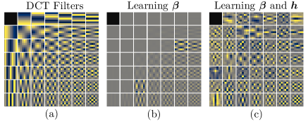
Figure 6.1: The DCT filter bank and example learned filters for (Ex) with training data from the “cameraman” image. (a) The 48 non-constant $7\times 7$ DCT filters used to initialize $\bm{\upgamma}$. The dark, top-left square represents the removed DC filter. (b) The DCT filters multiplied by their respective tuning parameter $\beta_{k}$ when ${\bm{\upgamma}}={\bm{\beta}}$. The range of $e^{\beta_{0}+\beta_{k}}$ is 0.001-1.08. The learned tuning parameters emphasize the higher-frequency DCT filters. (c) Learned filters when ${\bm{\upgamma}}=({\bm{\beta}},{\bm{h}})$ (scaled to have unit-norm for visualization).

A slight variation on learning the filters is to learn coefficients for a linear combination of filter basis elements [samuel:2009:learningoptimizedmap, chen:2014:insightsanalysisoperator], i.e., learning $a_{k,i}$ where

$${\bm{c}}_{k}=\sum_{i}a_{k,i}{\bm{b}}_{i},$$

for some set of basis filter elements, ${\bm{b}}_{i}$. One benefit of imposing a filter basis is the ability to ensure the filters lie in a given subspace. For example, [samuel:2009:learningoptimizedmap, chen:2014:insightsanalysisoperator] use the DCT as a basis and remove the constant filter so that all learned filters are guaranteed to have zero-mean.

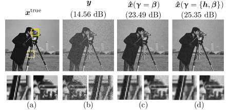
Figure 6.2: Example denoising results for the full “cameraman” test image and two of the training patches. (a) Noiseless training “cameraman” test image. (b) Noisy image and its SNR. (c) Denoised image using the learned tuning parameters that weight the DCT filters as shown in Fig. 6.1b. (d) Denoised image using the learned filter coefficients and tuning parameters as shown in Fig. 6.1c. For comparison, the denoised image using BM3D [dabov:2007:imagedenoisingsparse] has a SNR of 26.87. See Appendix D.2 for more details.

In terms of sparsifying functions, [peyre:2011:learninganalysissparsity, fehrenbach:2015:bilevelimagedenoising] used the same corner rounded 1-norm as in (CR1N), [samuel:2009:learningoptimizedmap] used $\phi=\text{log}\left(1+z^{2}\right)$ to relate their method to the Field of Experts framework [roth:2005:fieldsexpertsframework], [holler:2018:bilevelapproachparameter] used a quadratic penalty, and [kunisch:2013:bileveloptimizationapproach, chen:2014:insightsanalysisoperator] both consider multiple $\phi$ options to examine the impact of non-convexity in $\phi$. Ref. [kunisch:2013:bileveloptimizationapproach] compared $p$-norms, $\left\lVert{\bm{c}}_{k}\circledast{\bm{x}}\right\rVert_{p}^{p}$, for $p\in\{\tfrac{1}{2},1,2\}$, where the $p=\tfrac{1}{2}$ and $p=1$ cases are corner-rounded to ensure $\phi$ is smooth. (The $p=\tfrac{1}{2}$ case is non-convex.) Ref. [chen:2014:insightsanalysisoperator] compared the convex corner-rounded 1-norm in (CR1N) with two non-convex choices: the log-sum penalty $\text{log}\left(1+z^{2}\right)$, and the Student-t function $\text{log}\left(10\epsilon+\sqrt{z^{2}+\epsilon^{2}}\right)$.

Both [kunisch:2013:bileveloptimizationapproach, chen:2014:insightsanalysisoperator] found that non-convex penalty functions led to denoised images with better (higher) PSNR. They hypothesize that the improvement is due to the non-convex penalty functions better matching the heavy-tailed distributions in natural images. As further evidence of the importance of non-convexity, [chen:2014:insightsanalysisoperator] found that untrained $7\times 7$ DCT filters (excluding the constant filter) with learned tuning parameters and a non-convex $\phi$ outperformed learned filter coefficients with a convex $\phi$, despite the increased data adaptability when learning filter coefficients. The trade-off for using non-convex penalty functions is the possibility of local minimizers of the lower-level cost.

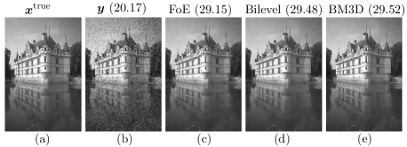
Figure 6.3: Example denoising results from [chen:2014:insightsanalysisoperator] comparing filters learned using bilevel methods to other denoising methods. (a) The original image ${\bm{x}}^{\text{true}}$. (b) The noisy image $\bm{y}$. (c-d) Denoised images using FoE [roth:2005:fieldsexpertsframework], BM3D [dabov:2007:imagedenoisingsparse], and a bilevel approach using a set-up equivalent to (Ex) with a non-convex penalty function, $\phi(z)=\text{log}\left(1+z^{2}\right)$ [chen:2014:insightsanalysisoperator]. The PSNR values in dB are given in parenthesis. ©2014 IEEE. Reprinted, with permission, from [chen:2014:insightsanalysisoperator].

chen:2014:insightsanalysisoperator also investigated how the number of learned filters and the size of the filters impacted denoising PSNR. They concluded that increasing the number of filters to achieve an over-complete filter set may not be worth the increased computational expense and that increasing the filter size past $11\times 11$ is unlikely to improve PSNR. Using 48 filters of size $7\times 7$ and the log-sum penalty function, [chen:2014:insightsanalysisoperator] achieved denoising results on natural images comparable to algorithms such as BM3D [dabov:2007:imagedenoisingsparse], as seen in Fig. 6.3. Although results will vary between applications and training data sets, the results from [chen:2014:insightsanalysisoperator] provide motivation for filter learning and an initial guide for designing bilevel methods.

In addition to variations on the running example for $\Upphi$ (6.1), a common regularizer for the lower-level cost is Total Generalized Variation with order 2 (TGV²) [bredies:2010:totalgeneralizedvariation]. Whereas TV encourages images to be piece-wise constant, TGV² is a generalization of TV designed for piece-wise linear images. Another generalization of TV for piece-wise linear images is Infimal Convolutional Total Variation (ICTV) [chambolle:1997:imagerecoverytotal]. Bilevel papers that investigate ICTV include [delosreyes:2017:bilevelparameterlearning, calatroni:2017:bilevelapproacheslearning]; these papers also investigate TGV². See [benning:2013:higherordertvmethods] for a comparison of the two.

TGV cost functions are typically expressed in the continuous domain, at least initially, but then discretized for implementation, e.g., [knoll:11:sot, setzer:11:icr]. One discrete approximation of the TGV² regularizer is:

$$R_{\mathrm{TGV}}({\bm{x}})=\operatorname*{min}_{{\bm{z}}}e^{\beta_{1}}\left\lVert{\bm{c}}_{\mathrm{TV}}\circledast{\bm{x}}-{\bm{z}}\right\rVert_{1}+e^{\beta_{2}}\left\lVert\partial{\bm{z}}\right\rVert_{1},$$

where ${\bm{c}}_{\mathrm{TV}}$ is a filter that takes finite differences and $\partial$ is a filter that approximates a symmetrized gradient. In TV, one usually thinks of $\bm{z}$ as a sparse vector; here $\bm{z}$ is a vector whose finite differences are sparse, so $\bm{z}$ is approximately piece-wise constant. Encouraging $\bm{z}$ to be piece-wise constant in turn makes $\bm{x}$ approximately piece-wise linear, since ${\bm{c}}_{\mathrm{TV}}\circledast{\bm{x}}\approx{\bm{z}}$ from the first term. Bilevel methods for learning $\beta_{1}$ and $\beta_{2}$ for the TGV² regularizer include [delosreyes:2017:bilevelparameterlearning, calatroni:2017:bilevelapproacheslearning]. An extension to the TGV² regularizer model is to learn a space-varying tuning parameter [hintermuller:2020:dualizationautomaticdistributed].

As an example of how the regularizer should be chosen based on the application, [hintermuller:2020:dualizationautomaticdistributed] found that standard TV with a learned tuning parameter performed best (in terms of SSIM) for approximately piece-wise constant images while TGV² with learned tuning parameters performed best for approximately piece-wise linear images.

6.2 Upper-Level Loss Function Design

From some of the earliest bilevel methods, e.g., [haber:2003:learningregularizationfunctionals, peyre:2011:learninganalysissparsity], to some of the most recent bilevel methods, e.g., [kobler:2021:totaldeepvariation, antil:2020:bileveloptimizationdeep], square error or mean squared error (MSE) remains the most common upper-level loss function. In the unsupervised setting, [zhang:2020:bilevelnestedsparse, deledalle:2014:steinunbiasedgradient] used SURE (an estimate of the MSE, see Section 3.1) as the upper-level loss function. Unlike many perceptually motivated image quality measures, MSE is convex in $\bm{x}$ and it is easy to find $\nabla_{\bm{x}}\ell({\bm{\upgamma}}\,;{\bm{\hat{x}}}({\bm{\upgamma}}))$. However, MSE does not capture perceptual quality nor image utility (see Section 3.1). This section discusses a few bilevel methods that used different loss functions.

Ref. [delosreyes:2017:bilevelparameterlearning] compared a squared error upper-level loss function with a Huber (corner rounded 1-norm) loss function. The corresponding lower-level problem was a denoising problem with a standard 2-norm data-fit term and three different options for a regularizer: TV, TGV², and ICTV. The authors learned tuning parameters for a natural image dataset using both upper-level loss function options for each of the lower-level regularizers.

Since SNR is equivalent to MSE, the MSE loss will always perform the best according to any SNR-based metric (assuming the bilevel model is well-trained). However, [delosreyes:2017:bilevelparameterlearning] found the tuning parameters learned using the Huber loss yielded denoised images with better qualitative properties and better SSIM, especially at low noise levels. Like MSE, the Huber loss operates point-wise and is easy to differentiate. Thus, the authors conclude that the Huber loss is a good trade-off between tractability and improving on MSE as an image quality measure.

A set of loss functions in [fehrenbach:2015:bilevelimagedenoising, hintermuller:2020:dualizationautomaticdistributed, sixou:2020:adaptativeregularizationparameter] consider the unsupervised or “blind” bilevel setting, where one wishes to reconstruct an image without clean samples. Therefore, rather than using an image quality metric that compares a reconstructed image, ${\bm{\hat{x}}}$, to some true image, ${\bm{x}}^{\text{true}}$, these loss function consider the estimated residual,

$$\hat{{\bm{n}}}=\hat{{\bm{n}}}({\bm{\upgamma}})={\bm{A}}{\bm{\hat{x}}}({\bm{\upgamma}})-{\bm{y}},$$

where $\bm{\upgamma}$ is learned using only noisy data. Unsupervised bilevel methods may be beneficial when there is no clean data and one has more knowledge of noise properties than of expected image content. All three methods [fehrenbach:2015:bilevelimagedenoising, hintermuller:2020:dualizationautomaticdistributed, sixou:2020:adaptativeregularizationparameter] assume the noise variance, $\sigma^{2}$, is known.

The earliest example [fehrenbach:2015:bilevelimagedenoising], learned tuning parameters $\bm{\upgamma}$ such that $\hat{{\bm{n}}}$ matched the second moment of the assumed Gaussian distribution for the noise. Their lower-level cost is comparable to (Ex), but re-written in terms of $\bm{n}$ and with pre-defined finite differencing or $5\times 5$ DCT filters, i.e., they learn only the tuning parameters, $\beta_{k}$. Their upper-level loss encourages the empirical variances of the noise in different frequency bands to match the expected variances:

$$\ell({\bm{\upgamma}}\,;{\bm{n}}({\bm{\upgamma}}))=\dfrac{1}{2}\sum_{i}\frac{\left(\left\lVert{\bm{f}}_{i}\circledast{\bm{n}}\right\rVert^{2}_{2}-\mu_{i}\right)^{2}}{v_{i}}$$

$$\mu_{i}=\mathbb{E}\left[\left\lVert{\bm{f}}_{i}\circledast{\bm{n}}\right\rVert^{2}_{2}\right]\text{ and }v_{i}=\text{Var}\left[\left\lVert{\bm{f}}_{i}\circledast{\bm{n}}\right\rVert^{2}_{2}\right],$$

where ${\bm{f}}_{i}$ are predetermined filters that select specific frequency components. By using bandpass filters that partition Fourier space, the corresponding means and variances of the second moments of the filtered noise are easily computed, with

$$\mu_{i}=N\sigma^{2}\left\lVert{\bm{f}}_{i}\right\rVert^{2}\quad\text{ and }\quad v_{i}=N\sigma^{4}\left\lVert{\bm{f}}_{i}\right\rVert^{4}.$$

Although the experimental results are promising, [fehrenbach:2015:bilevelimagedenoising] does not claim state-of-the-art results since their lower-level denoiser is relatively simple.

As an alternative to the Gaussian-inspired approach in [fehrenbach:2015:bilevelimagedenoising], [hintermuller:2020:dualizationautomaticdistributed] and [sixou:2020:adaptativeregularizationparameter] use loss functions that penalize noise outside a set “noise corridor.” Both methods learn space-varying tuning parameters, and the upper-level loss consists of a data-fit term (that measures noise properties) and a regularizer on $\bm{\upgamma}$. The data-fit term in the upper-level loss function in [fehrenbach:2015:bilevelimagedenoising] defines the noise corridor between a maximum variance, $\bar{\sigma}^{2}$, and a minimum variance, $\underline{\sigma}^{2}$:

$$\bm{1}^{\prime} F.\left({\bm{w}}\odot({\bm{n}}({\bm{\upgamma}})\odot{\bm{n}}({\bm{\upgamma}}))\right)\text{ for }$$

$$F(n)=\dfrac{1}{2}\text{max}(n-\bar{\sigma}^{2},0)^{2}+\dfrac{1}{2}\text{min}(n-\underline{\sigma}^{2},0)^{2},$$ (6.2)

where $\bm{w}$ is a predetermined weighting vector. The noise corridor function, $F(n)$, penalizes any noise outside of the expected range as shown in Fig. 6.4. Ref. [sixou:2020:adaptativeregularizationparameter] uses the same noise corridor function, but extends the bilevel method for images with Poisson noise; [sixou:2020:adaptativeregularizationparameter] thus estimates the noisy image using the Kullback-Leibler distance. In addition to the noise corridor function as the data-fit component of the upper-level loss function, [hintermuller:2020:dualizationautomaticdistributed, sixou:2020:adaptativeregularizationparameter] include a smoothness-promoting regularizer on $\bm{\upgamma}$, which is a spatially varying tuning parameter vector in both methods.

Figure 6.4: Noise corridor function (6.2) used as part of the upper-level loss function for the unsupervised bilevel method in [hintermuller:2020:dualizationautomaticdistributed].

The task-based nature of bilevel typically makes regularizers or constraints on $\bm{\upgamma}$ unnecessary (see Section 7.4 for common options for other forms of learning). However, there are two general cases where a regularizer on $\bm{\upgamma}$ is useful in the upper-level loss function. First, a regularizer can help avoid over-fitting when the amount of training data is insufficient for the number of learnable hyperparameters. This is often the case when learning space-varying parameters that have similar dimensions as the input data, e.g., [haber:2003:learningregularizationfunctionals, delia:2020:bilevelparameteroptimization, hintermuller:2020:dualizationautomaticdistributed, sixou:2020:adaptativeregularizationparameter]. In such cases, the regularization often takes the form of a 2-norm on the learned hyperparameters, $\left\lVert{\bm{\upgamma}}\right\rVert^{2}_{2}$.

Second, some problems require application-specific constraints, e.g., [chambolle:2021:learningconsistentdiscretizations] incorporates constraints in the upper-level loss to ensure that the learned parameters are valid interpolation kernels. Many other hyperparameter constraints do not require a regularization term, For example, non-negativity constraints on tuning parameters are easily handled by redefining the tuning parameter in terms of an exponential, as in (Ex), and box constraints are common and easy to incorporate with a projection step if using a gradient-based method. Constraints that require sparsity on the learned parameters may benefit from regularization in the upper-level loss function.

An example of an application-specific constraint is found in [ehrhardt:2021:inexactderivativefreeoptimization, sherry:2020:learningsamplingpattern], which consider MRI reconstruction with a data-fit term and a variational regularizer. Both papers extend the bilevel model in (Ex) to include part of the forward model in the learnable parameters, $\bm{\upgamma}$. Specifically, [ehrhardt:2021:inexactderivativefreeoptimization, sherry:2020:learningsamplingpattern] learned the sparse sampling matrix for MRI. (Ref. [sherry:2020:learningsamplingpattern] additionally learns tuning parameters for predetermined filters, whereas [ehrhardt:2021:inexactderivativefreeoptimization] sets the tuning parameters and filters and learns only the sampling matrix.) Here, the forward model is

$${\bm{A}}=\mathrm{diag}\Big{(}\underbrace{s_{1},s_{2},\ldots,s_{M}}_{{\bm{s}}({\bm{\upgamma}})}\Big{)}{\bm{F}},$$

where $\bm{F}$ is the DFT matrix and $s_{i}$ are learned binary values that specify whether a frequency location should be sampled.

The motivation for learning a sparse sampling matrix comes from the lower-level MRI reconstruction problem; designing more effective sparse sampling patterns in MRI can decrease scan time and thus improve patient experience, decrease cost, and decrease artifacts from patient movement. This goal requires the learned parameters, $s_{i}$, to be binary, which in turn influences the upper-level loss function design. Thus, [ehrhardt:2021:inexactderivativefreeoptimization, sherry:2020:learningsamplingpattern] include regularization in the upper-level to encourage $\bm{s}$ to be sparse, e.g., [sherry:2020:learningsamplingpattern] uses an upper-level loss with a squared error term and regularizer on $\bm{s}$:

$$\ell({\bm{\upgamma}}\,;{\bm{\hat{x}}}({\bm{\upgamma}}))=\|{\bm{\hat{x}}}({\bm{\upgamma}})-{\bm{x}}^{\text{true}}\|^{2}_{2}+\lambda\sum_{i}\left(s_{i}+s_{i}(1-s_{i})\right),$$ (6.3)

where $\lambda$ is a upper-level tuning parameter that one must set manually. (In experiments, they thresholded the learned $s_{i}$ values to be exactly binary.) An alternative approach is to constrain the number of samples [gozcu:18:lbc], though that formulation requires other optimization methods.

6.3 Conclusion

This section split the discussion of lower-level cost and upper-level loss functions to discuss trends in both areas. However, when designing a bilevel problem, design decisions can impact both levels. For example, the unsupervised nature of [fehrenbach:2015:bilevelimagedenoising, sixou:2020:adaptativeregularizationparameter] clearly impacted their choice of upper-level loss function to use noise statistics rather than squared error calculated with ground-truth data. Since it can be challenging to learn many good parameters from noisy training data, the unsupervised nature also likely impacted the authors’ decision to learn only tuning parameters and set the filters manually. Another example of coupling between lower-level and upper-level design is when one enforces application-specific constraints on the learned parameters, e.g., using a regularizer like (6.3) in the upper-level loss to promote sparsity of the MRI sampling matrix [ehrhardt:2021:inexactderivativefreeoptimization, sherry:2020:learningsamplingpattern].

In addition to design decisions influencing both levels, bilevel methods may adopt common techniques for the upper-level loss function and lower-level cost function. For example, a common theme is the tendency to use smooth functions, such as replacing the 1-norm with a corner-rounded 1-norm. This approach requires setting a smoothing parameter, e.g., $\epsilon$ in (CR1N), which in turn impacts the Lipschitz constant and optimization speed. More accurate approximations generally lead to larger Lipschitz constants and slower convergence. One approach to trading-off the accuracy of the smoothing with optimization speed is to use a graduated approach and approximate the non-smooth term more and more closely as the optimization progresses [chen:2021:learnabledescentalgorithm].

The prevalence of smoothing is unsurprising considering that this review focuses on gradient-based bilevel methods. Rare exceptions include [mccann:2020:supervisedlearningsparsitypromoting, ghosh:2021:bilevellearningl1regularizers], which used the (not corner-rounded) one-norm to define $\phi$ to learn convolutional filters using the translation to a single level approach described in Section 4.3. The impact of smoothing and how accurately one should approximate a non-differentiable point remains an open question.

From an image quality perspective, ideally one would independently design the lower-level cost function and upper-level training loss. The lower-level cost would depend on the imaging physics and would incorporate regularizers that expected to provide excellent image quality when tuned appropriately, and the upper-level loss would use terms that are meaningful for the imaging tasks of interest. As we have seen, in practice one often makes compromises to facilitate optimization and reduce computation time.

Chapter 7 Connections and Future Directions

This final section connects bilevel methods with related approaches and mentions some additional future directions beyond those already described in previous sections.

Shlezinger et al. [shlezinger:2020:modelbaseddeeplearning] recently proposed a framework, summarized in Fig. 7.1, for categorizing learning-based approaches that combine inferences, or prior knowledge, and deep learning. Inferences can include information about the structure of the forward model, $\bm{A}$, or about the object $\bm{x}$ being imaged. For example, any known statistical properties of the object of interest could be used to design a regularizer that encourages the minimizer ${\bm{\hat{x}}}$ to be compatible with that prior information. At one extreme, inference-based approaches rely on a relatively small number of handcrafted regularizers with a few, if any, tuning parameters learned from training data. At the other extreme, fully learned approaches assume no information about the application or data and learn all hyperparameters from training data.

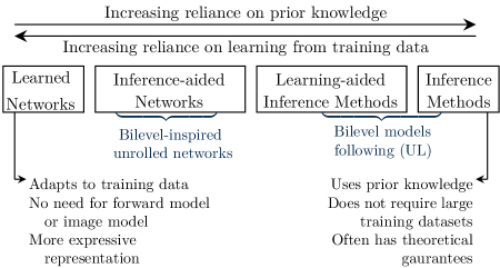
Figure 7.1: Spectrum of learning to inference-based methods from [shlezinger:2020:modelbaseddeeplearning].

Ref. [shlezinger:2020:modelbaseddeeplearning] proposed two general categories for methods that mix elements of inference-based and learning-based methods. The first category, inference-aided networks, includes deep neural networks (DNNs) with architectures based on an inference-based method. For example, in deep unrolling, one starts with a fixed number of iterations of an optimization algorithm derived from a cost function and then learns parameters that may vary between iterations, or “layers,” or may be shared across such iterations. Section 7.1 further discusses unrolling, which is a common inference-aided network design strategy, and the connection to the bilevel unrolling method described in Section 4.4.

The second general category is DNN-aided inference methods [shlezinger:2020:modelbaseddeeplearning]. These methods incorporate a deep learning component into traditional inference-based techniques (typically a cost function in image reconstruction). The learned DNN component(s) can be trained separately for each iteration or end-to-end. Because prior knowledge takes a larger role than in the inference-aided networks, these methods typically require smaller training datasets, with the amount of training data required varying with the number of hyperparameters. Section 7.3 discusses how bilevel methods compare to Plug-and-Play, which is an example DNN-aided inference model.

While [shlezinger:2020:modelbaseddeeplearning] focused on DNNs due to their highly expressive nature and the abundance of interest in them, the idea of trading off prior knowledge and learning components applies to machine learning more broadly. Section 7.1 through 7.3 describe how bilevel methods fit into the framework from [shlezinger:2020:modelbaseddeeplearning] and relate bilevel methods to other methods in the framework. Although not covered in the above framework, Section 7.4 also compares bilevel methods to a third general category: “single-level” hyperparameter learning methods. Like bilevel methods, single-level methods learn hyperparameters in a supervised manner. However, they generally learn parameters that sparsify the training images, $\{{\bm{x}}^{\text{true}}_{j}\}$, and do not use the noisy data, $\{{\bm{y}}_{j}\}$. This last comparison demonstrates the benefit of task-based approaches. Of course, there is variety among bilevel methods; this discussion is meant to provide perspective and general relations to increase understanding, rather than to narrow the definition or application of any method.

7.1 Connection: Learnable Optimization Algorithms

Learning parameters in unrolled optimization algorithms to create an inference-aided network, often called a Learnable Optimization Algorithm (LOA), is a quickly growing area of research [monga:2021:algorithmunrollinginterpretable]. The first such instance was a learned version of the Iterative Shrinkage and Thresholding Algorithm (ISTA), called LISTA [gregor:10:lfa]. Similar to the bilevel unrolling method, a LOA typically starts from a traditional, inference-based optimization algorithm, unrolls multiple iterations, and then learns parameters using end-to-end training.

There are many unrolled methods for image reconstruction [monga:2021:algorithmunrollinginterpretable]. Two examples that explicitly state the bilevel connection are [chen:2021:learnabledescentalgorithm, bian:2020:deepparallelmri]; both set-up a bilevel problem with a DNN as a regularizer and then allow the parameters to vary by iteration, i.e., learning ${{\bm{c}}_{k}^{(t)}}$ where $t$ denotes the lower-level iteration. Ref. [bian:2020:deepparallelmri] motivated the use of an unrolled DNN over more inference-based methods by the lack of an accurate forward model, specifically coil sensitivity maps, for MRI reconstruction. Other examples of unrolled networks are [hammernik:2018:learningvariationalnetwork], which unrolls the Field of Experts model [roth:2005:fieldsexpertsframework] (see Sections 2.3 and 6.1 for how the Field of Experts model has inspired many bilevel methods); [lim:2020:improvedlowcountquantitative], which unrolls the convolutional analysis operator model [chun:2020:convolutionalanalysisoperator] (see (2.12)); and [franceschi:2018:bilevelprogramminghyperparameter], which discusses the connection to meta-learning.

Unlike the unrolled approach to bilevel learning described in Section 4.4, many LOAs depart from their base cost function and “only superficially resemble the steps of optimization algorithms” [chen:2021:learnabledescentalgorithm]. For example, unrolled algorithms may “untie” the gradient from the original cost function, e.g., using $\widetilde{{\bm{A}}}^{\prime}({\bm{A}}{\bm{x}}-{\bm{y}})$, instead of ${\bm{A}}^{\prime}({\bm{A}}{\bm{x}}-{\bm{y}})$ for the gradient of the common 2-norm data-fit term, where $\tilde{{\bm{A}}}^{\prime}$ is learned or otherwise differs from the adjoint of $\bm{A}$. LOAs that allow the learned parameters to vary every unrolled iteration or learn step size and momentum parameters further depart from a cost function perspective.

In addition to selecting which variables to learn, one must decide how many iterations to unroll for both bilevel unrolled approaches and LOAs. Most methods pick a set number of iterations in advance, perhaps based on previous experience, initial trials, or the available computational resources. Using a set number of iterations yields an algorithm with predictable run times and allows the learned parameters to adapt to the given number of iterations. Further, picking a small number of iterations can act as implicit regularization, comparable to early stopping in machine learning, which may be helpful when the amount of training data is small relative to the number of hyperparameters in the unrolled algorithm [franceschi:2018:bilevelprogramminghyperparameter].

One can also use a convergence criteria to determine the number of iterations to evaluate, rather than selecting a number in advance [antil:2020:bileveloptimizationdeep]. This convergence-based method more closely follows classic inference-based optimization algorithms. A benefit of running the lower-level optimization algorithm until convergence is that one could switch optimization algorithms between training and testing, especially for strictly convex lower-level cost functions, and still expect the learned parameters to perform similarly. This ability to switch optimization algorithms means one could use faster, but not differentiable, algorithms at test-time, such as accelerated gradient descent methods with adaptive restart [kim:18:aro]. We are unaware of any bilevel methods that have exploited this possibility.

Even within the unrolling methodology, one must make several design decisions. To remain most closely tied to the original optimization algorithm, an unrolled method might fix a large number of iterations or run the optimization algorithm until convergence, use the same parameters every layer, and calculate the step size based on the Lipschitz constant every upper-level iteration (see discussion in Section 4.4.1). Like all design decisions, there are trade-offs and the literature shows many successful methods that benefit from the increased generality of designing LOAs that are further removed from their cost function roots [monga:2021:algorithmunrollinginterpretable]. Echoing the ideas from [shlezinger:2020:modelbaseddeeplearning], the design should be based on the specific application and relative availability, reliability, and importance of prior knowledge and training data.

This survey focuses on unrolled methods that are closely tied to the original bilevel formulation; [monga:2021:algorithmunrollinginterpretable] reviews LOAs more broadly. A benefit of maintaining the connection to the original cost function and optimization algorithm is that, once trained, the lower-level problem in an unrolled bilevel method inherits any theoretical and convergence results from the corresponding optimization method. The corresponding benefit for LOAs is increased flexibility in network architecture.

7.2 Connection: Equilibrium-based Networks

Equilibrium-based, or fixed point, networks are related to both LOAs and the minimizer approach from Section 4.2. The idea was proposed only recently in [bai:2019:deepequilibriummodels], but has received much attention. From the unrolled perspective, equilibrium networks consider what happens when the number of unrolled iterations approaches infinity. Alternatively, they can be viewed as a single, implicit layer; as in the minimizer approach, the output is the solution to a nonlinear equation.

We first consider the unrolled perspective. If an algorithm $\Psi$ is a contraction, i.e.,

$$\left\lVert\Psi({\bm{x}}_{1}\,;\,{\bm{\upgamma}})-\Psi({\bm{x}}_{2}\,;\,{\bm{\upgamma}})\right\rVert\leq\delta\left\lVert{\bm{x}}_{1}-{\bm{x}}_{2}\right\rVert,\,\forall{\bm{x}}_{1},{\bm{x}}_{2}\in\mathbb{F}^{N}$$

for some parameter $\delta\in[0,1)$, then the sequence of iterates will eventually converge to a fixed-point of $\Psi$. If the optimization algorithm optimizes a cost function with a data-fit and regularization term, then the equilibrium network approach is equivalent to a bilevel method. For a given value of $\bm{\upgamma}$, the contraction condition is typically easy to satisfy by selecting an appropriate step-size in algorithms like gradient descent. Ref. [gilton:2021:deepequilibriumarchitectures] provides conditions on deep equilibrium models specific to optimization algorithms based on gradient descent, proximal gradient descent, and ADMM that ensure convergence.

Re-using some of our bilevel notation, let ${\bm{\hat{x}}}({\bm{\upgamma}})$ denote a fixed-point of an equilibrium network. The derivation for finding $\nabla_{\bm{\upgamma}}{\bm{\hat{x}}}({\bm{\upgamma}})\in\mathbb{F}^{N\times R}$ follows similar steps to the IFT perspective on the bilevel minimizer approach in Section 4.2.1. The key difference is that rather than using the first-order optimally condition as in the minimizer approach (4.3), the equilibrium method considers the lower-level minimizer to be a fixed point of an optimization algorithm.

When the goal of the lower level problem is to find a fixed point, the bilevel problem becomes

$$\operatorname*{argmin}_{\bm{\upgamma}} \underbrace{\ell\left({\bm{\upgamma}}\,;\,{\bm{\hat{x}}}({\bm{\upgamma}})\right)}_{\ell({\bm{\upgamma}})}\text{ s.t. }\underbrace{{\bm{\hat{x}}}({\bm{\upgamma}})=\Psi({\bm{\hat{x}}}({\bm{\upgamma}})\,;{\bm{\upgamma}})}_{\text{Fixed point equation}}.$$ (7.1)

Similar to the IFT perspective, one can differentiate both sides of the fixed point equation using the chain rule

$$\nabla_{\bm{\upgamma}}{\bm{\hat{x}}}({\bm{\upgamma}}) =\left(\nabla_{\bm{x}}\Psi({\bm{\hat{x}}}({\bm{\upgamma}})\,;{\bm{\upgamma}})\right)\nabla_{\bm{\upgamma}}{\bm{\hat{x}}}({\bm{\upgamma}})+\nabla_{\bm{\upgamma}}\Psi({\bm{\hat{x}}}({\bm{\upgamma}})\,;{\bm{\upgamma}})$$

and then rearrange to derive an expression for $\nabla_{\bm{\upgamma}}{\bm{\hat{x}}}({\bm{\upgamma}})$

$$\nabla_{\bm{\upgamma}}{\bm{\hat{x}}}({\bm{\upgamma}}) =(\bm{I}-\underbrace{\left(\nabla_{\bm{x}}\Psi({\bm{\hat{x}}}({\bm{\upgamma}})\,;{\bm{\upgamma}})\right)}_{\hat{{\bm{J}}}})^{\text{-}1}\nabla_{\bm{\upgamma}}\Psi({\bm{\hat{x}}}({\bm{\upgamma}})\,;{\bm{\upgamma}}).$$ (7.2)

The matrix $\hat{{\bm{J}}}$ is the Jacobian of the optimization algorithm, evaluated at the fixed point ${\bm{\hat{x}}}({\bm{\upgamma}})$.

Substituting (7.2) into the expression for the upper-level gradient (4.2) yields

$$\nabla\ell({\bm{\upgamma}}) =\nabla_{\bm{\upgamma}}\ell({\bm{\upgamma}}\,;{\bm{\hat{x}}}({\bm{\upgamma}}))+\left(\nabla_{\bm{\upgamma}}\Psi({\bm{\hat{x}}}({\bm{\upgamma}})\,;{\bm{\upgamma}})\right)^{\prime}(\bm{I}-\hat{{\bm{J}}})^{\text{-}1}\nabla_{\bm{x}}\ell({\bm{\upgamma}}\,;{\bm{\hat{x}}}({\bm{\upgamma}})).$$ (7.3)

If the optimization is standard gradient descent, i.e., $\Psi({\bm{x}}\,;{\bm{\upgamma}})={\bm{x}}-\alpha_{\Upphi}\nabla_{{\bm{x}}}\Upphi({\bm{x}}\,;{\bm{\upgamma}})$, then

$$\nabla_{\bm{\upgamma}}\Psi({\bm{\hat{x}}}({\bm{\upgamma}})\,;{\bm{\upgamma}}) =\text{-}\alpha_{\Upphi}\nabla_{{\bm{x}}{\bm{\upgamma}}}\Upphi({\bm{x}}\,;{\bm{\upgamma}})\text{ and }$$

$$\nabla_{\bm{x}}\Psi({\bm{\hat{x}}}({\bm{\upgamma}})\,;{\bm{\upgamma}}) =\bm{I}-\alpha_{\Upphi}\nabla_{{\bm{x}}{\bm{x}}}\Upphi({\bm{x}}\,;{\bm{\upgamma}}).$$

Substituting these expressions into (7.2) yields the gradient as derived using the IFT perspective in the minimizer approach (4.5), showing the close connection between the equilibrium and minimizer approach.

Similar to the minimizer approach, one can use any algorithm to find a fixed point ${\bm{\hat{x}}}({\bm{\upgamma}})$ of $\Psi$. For example, [bai:2019:deepequilibriummodels] used a quasi-Newton method and [gilton:2021:deepequilibriumarchitectures] used a standard fixed-point accelerated method. One can use any fixed point algorithm to find ${\bm{\hat{x}}}({\bm{\upgamma}})$; the algorithm used need not correspond to $\Psi$ in (7.1). For example, $\Psi$ could be standard gradient descent, even if one uses a more advanced algorithm to initially compute ${\bm{\hat{x}}}({\bm{\upgamma}})$. Another similarity to the minimizer approach is that the learned parameters are optimal at convergence of the lower-level problem, rather than after a fixed number of lower-level iterations. Therefore, the end-user can trade-off accuracy and compute requirements at test time, unlike in unrolled approaches where the number of iterations is pre-decided.

Although the equilibrium model is the limit as the number of unrolled iterations approaches infinity, computing $\nabla\ell({\bm{\upgamma}})$ does not require backpropagation nor storing any intermediate matrices. The trade-off is that (7.3) requires multiplying $(\bm{I}-\hat{{\bm{J}}})^{\text{-}1}$ by a vector. The remaining computations in the full upper-level gradient (7.3) are straightforward. Similar to the required Hessian inverse-vector product in the minimizer approach, one can use an iterative algorithm to approximate the matrix inverse. Ref. [gilton:2021:deepequilibriumarchitectures] notes that the inverse matrix-vector product

$${\bm{v}}=(\bm{I}-\hat{{\bm{J}}})^{\text{-}1}\nabla_{\bm{x}}\ell({\bm{\upgamma}}\,;{\bm{\hat{x}}}({\bm{\upgamma}})),$$

is a fixed point of the equation

$${\bm{v}}=\hat{{\bm{J}}}{\bm{v}}+\nabla_{\bm{x}}\ell({\bm{\upgamma}}\,;{\bm{\hat{x}}}({\bm{\upgamma}})).$$

Therefore, one can use any fixed-point solver to compute the matrix-vector product. Another way to decrease the computational cost of the Jacobian product is to use the method from [ramzi:2021:shinesharinginverse]: if a quasi-Newton algorithm is used to estimate the Jacobian for the forward step of computing ${\bm{\hat{x}}}({\bm{\upgamma}})$, then one can “re-use” this estimated Jacobian to find $\nabla\ell({\bm{\upgamma}})$.

Fixed point networks can also be viewed from the perspective of unrolled methods. Although it is often infeasible to backpropagate through the large number of iterations required to reach a fixed point, backpropagating through the last few iterations yields a valid gradient estimate for $\nabla_{\bm{\upgamma}}{\bm{\hat{x}}}({\bm{\upgamma}})$ [shaban:2019:truncatedbackpropagationbilevel]. Ref. [shaban:2019:truncatedbackpropagationbilevel] proves that this “truncated backpropagation” approach converges to a stationary point of the upper-level loss when the lower-level cost function is locally strongly convex around ${\bm{\hat{x}}}({\bm{\upgamma}})$ because the backpropagation gradient error decays exponentially with reverse depth. A similar approach is to use ${\bm{\hat{x}}}({\bm{\upgamma}})$ at every backpropagation step rather than previous iterates. Ref. [lorraine:2020:optimizingmillionshyperparameters] shows this is equivalent to approximating the matrix inverse in the minimizer approach using a Neumann series.

Recently, [fung:2022:jfbjacobianfreebackpropagation] proposed a Jacobian-free method to find $\nabla\ell({\bm{\upgamma}})$ that takes the approach from [shaban:2019:truncatedbackpropagationbilevel] to the extreme case: it considers unrolling a single layer. The approach in [fung:2022:jfbjacobianfreebackpropagation] is equivalent to viewing the deep equilibrium network as a single layer network where the initialization is the fixed-point, i.e., using ${\bm{\hat{x}}}({\bm{\upgamma}})=\Psi({\bm{x}}^{(0)}\,;\,{\bm{\upgamma}})$ in the unrolled method with ${\bm{x}}^{(0)}={\bm{\hat{x}}}({\bm{\upgamma}})$. With this new perspective, it is easy to use existing backpropagation tools to compute the derivative through the single layer network. Assuming that the network is Lipschitz, contractive, and differentiable and that the upper-level loss is differentiable, [fung:2022:jfbjacobianfreebackpropagation] shows the Jacobian-free gradient is a descent direction for estimates of ${\bm{\hat{x}}}({\bm{\upgamma}})$ that are within some error bound of the true fixed point.

Deep equilibrium networks can be fully learned or they can incorporate physics-based models into their network architecture and move into the inference-aided networks category in Fig. 7.1. For example, [gilton:2021:deepequilibriumarchitectures, heaton:2021:feasibilitybasedfixedpoint] incorporated system matrices into fixed point networks and applied them to MRI and CT image reconstruction problems.

7.3 Connection: Plug-and-play Priors

The Plug-and-Play (PNP) framework [venkatakrishnan:2013:plugandplaypriorsmodel] is an example of a DNN-aided inference method. It is similar to bilevel methods in its dependence on the forward model. However, unlike bilevel methods, the PNP framework need not be connected to a specific lower-level cost function and it leverages pre-trained denoisers rather than training them for a specific task.

As a brief overview of the PNP framework, consider rewriting the generic data-fit plus regularizer optimization problem (2.1) with an auxiliary variable:

$${\bm{\hat{x}}}=\operatorname*{argmin}_{{\bm{x}}\in\mathbb{F}^{N}}\underbrace{\overbrace{d({\bm{x}}\,;{\bm{y}})}^{\text{Data-fit}}+\;\;\;\beta\overbrace{R({\bm{z}}\,;{\bm{\upgamma}})}^{\text{Regularizer}}}_{\Upphi({\bm{x}}\,;{\bm{\upgamma}})}\quad\text{ s.t. }{\bm{x}}={\bm{z}}.$$ (7.4)

Using ADMM [eckstein:92:otd] to solve this constrained optimization problem and rearranging variables yields the following iterative optimization approach for (7.4):

$${{\bm{x}}^{(u+1)}} =\operatorname*{argmin}_{\bm{x}}d({\bm{x}}\,;{\bm{y}})+\frac{\lambda}{2}\|{\bm{x}}-\underbrace{({{\bm{z}}^{(u)}}-{{\bm{u}}^{(u)}})}_{\tilde{{\bm{x}}}}\|^{2}_{2} =\text{prox}_{\frac{1}{\lambda}d({\bm{x}}\,;{\bm{y}})}(\tilde{{\bm{x}}})$$

$${{\bm{z}}^{(u+1)}} =\operatorname*{argmin}_{\bm{z}}\beta R({\bm{z}}\,;{\bm{\upgamma}})+\frac{\lambda}{2}\|{\bm{z}}-\underbrace{({{\bm{x}}^{(u)}}+{{\bm{u}}^{(u)}})}_{\tilde{{\bm{z}}}}\|^{2}_{2} =\text{prox}_{\frac{\beta}{\lambda}R({\bm{z}}\,;{\bm{\upgamma}})}(\tilde{{\bm{z}}})$$

$${{\bm{u}}^{(u+1)}} ={{\bm{u}}^{(u)}}+({{\bm{x}}^{(u+1)}}-{{\bm{z}}^{(u+1)}}),$$

where $\lambda$ is an ADMM penalty parameter that effects the convergence rate (but not the limit, for convex problems). The first step is a proximal update for $\bm{x}$ that uses the forward model but does not depend on the regularizer. Conversely, the second step is a proximal update for the split variable $\bm{z}$ that depends on the regularizer, but is agnostic of the forward model. This step acts as a denoiser. The final step is the dual variable update and encourages ${{\bm{x}}^{(u)}}\approx{{\bm{z}}^{(u)}}$ as $u\rightarrow\infty$.

The key insight from [venkatakrishnan:2013:plugandplaypriorsmodel] is that the above update equations separate the forward model and denoiser. Thus, one can substitute, or “plug in,” a wide range of denoisers for the $\bm{z}$ update, in place of its proximal update, while keeping the data-fit update independent.

Whereas in the original ADMM approach, the parameter $\lambda$ has no effect on the final image for convex cost functions, in the PNP framework that parameter does affect image quality. Thus, one could also use training data to tune the $\lambda$ in a bilevel manner. Although PNP allows one to substitute a pre-trained denoiser, one could additionally tune the parameters in the denoiser. Ref. [he:2019:optimizingparameterizedplugandplay] provides one such example of starting from a PNP framework then learning denoising parameters and $\lambda$ that vary by iteration.

A large motivation for the PNP framework is the abundance of advanced denoising methods, including ones that are not associated with an optimization problem such as BM3D [dabov:2007:imagedenoisingsparse]. However, using existing denoisers sacrifices the ability to learn parameters to work well with the specific forward model, as is done in task-based methods. As simple examples of how learned parameters may differ when $\bm{A}$ changes, [chambolle:2021:learningconsistentdiscretizations] found that different filters worked better for image denoising versus image inpainting and [effland:2020:variationalnetworksoptimal] found that unrolled deblurring methods required more upper-level iterations than unrolled denoising methods. A more complicated example is using bilevel methods to learn some aspect of $\bm{A}$ alongside some aspect of the regularizer, e.g., [sherry:2020:learningsamplingpattern] learned a sparse sampling matrix and tuning parameter for MRI that are adaptive to the regularization for the image reconstruction problem.

7.4 Connection: Single-Level Parameter Learning

Section 2.3 briefly discussed some approaches to learning analysis operators. This section further motivates the task-based bilevel set-up by discussing the filter learning constraints imposed in single-level hyperparameter learning methods.

As summarized in Section 2.3, the earliest methods for learning analysis regularizers had no constraints on the analysis operators. Those approaches learned filters from training data to make a prior distribution match the observed data distribution. In contrast, more recent approaches to filter learning minimize a cost function that requires either a penalty function or constraint on the operators to ensure filter diversity. For reference, the cost functions mentioned in Section 2.3 were:

$$\text{AOL}: \operatorname*{argmin}_{{\bm{\Omega}},\,{\bm{X}}}\left\lVert{\bm{\Omega}}{\bm{X}}\right\rVert_{1}+\frac{\beta}{2}\left\lVert{\bm{Y}}-{\bm{X}}\right\rVert^{2}\text{ s.t. }{\bm{\Omega}}\in\mathcal{S},$$

$$\text{TL}: \operatorname*{argmin}_{{\bm{\Omega}}\in\mathbb{F}^{S\times S},\,{\bm{X}}}\left\lVert{\bm{\Omega}}{\bm{Y}}-{\bm{X}}\right\rVert^{2}_{2}+R({\bm{\Omega}})\text{ s.t. }\left\lVert{\bm{X}}_{i}\right\rVert_{0}\leq\alpha\;\forall i,$$

$$\text{CAOL}: \operatorname*{argmin}_{[{\bm{c}}_{1},\ldots,{\bm{c}}_{K}]}\operatorname*{min}_{\bm{z}}\sum_{k=1}^{K}\dfrac{1}{2}\left\lVert{\bm{c}}_{k}\circledast{\bm{x}}-{\bm{z}}\right\rVert^{2}_{2}+\beta\left\lVert{\bm{z}}_{k}\right\rVert_{0}\text{ s.t. }[{\bm{c}}_{1},\ldots,{\bm{c}}_{K}]\in\mathcal{S},$$

where AOL is analysis operator learning [yaghoobi:2013:constrainedovercompleteanalysis], TL is transform learning [ravishankar:2013:learningsparsifyingtransforms], and CAOL is convolutional analysis operator learning [chun:2020:convolutionalanalysisoperator]. In the following discussion of constraint sets, the equivalent filter matrix for CAOL has the convolutional kernels as rows:

$${\bm{\Omega}}_{\mathrm{CAOL}}=\begin{bmatrix}{\bm{c}}_{1}^{\prime}\\ \vdots\\ {\bm{c}}_{K}^{\prime}\end{bmatrix}.$$

While there are many other proposed cost functions in the literature, using different norms or including additional variables, these three examples capture the most common structures for filter learning.

In all the above cost functions, if one removed the constraint or regularizer, then the trivial solution would be to learn zero filters for $\bm{\Omega}$. Furthermore, a simple row norm constraint on $\bm{\Omega}$ would be insufficient, as then the minimizer would contain a single filter that is repeated many times. (In contrast, a unit norm constraint typically suffices for dictionary learning.) A row norm constraint plus a full rank constraint is also insufficient because $\bm{\Omega}$ can have full rank while being arbitrarily close to the rank-1 case of having a single repeated row.

The choice of constraint set $\mathcal{S}$ is important in single-level learning. Many methods constrain analysis operators to satisfy a tight frame constraint. A matrix ${\bm{A}}$ is a tight frame if there is a positive constant, $\alpha$, such that

$$\left\lVert{\bm{A}}^{\prime}{\bm{x}}\right\rVert^{2}_{2}=\sum_{i}\lvert\langle{\bm{q}}_{i},{\bm{x}}\rangle\rvert^{2}=\alpha\left\lVert{\bm{x}}\right\rVert^{2}_{2},\;\forall{\bm{x}}$$

where ${\bm{q}}_{i}$ is the $i$th column of $\bm{A}$. This tight frame condition is equivalent to ${\bm{A}}{\bm{A}}^{\prime}=\alpha\bm{I}$ for some positive constant $\alpha$. Most analysis operators are defined with filters in their rows, so a tight frame requirement on the filters appears as the constraint ${\bm{\Omega}}^{\prime}{\bm{\Omega}}=\alpha\bm{I}$.

Under the tight frame constraint for the filters, $\bm{\Omega}$ must be square or tall, so the filters are complete or over-complete. However, [yaghoobi:2013:constrainedovercompleteanalysis] found that the frame constraint was insufficient when learning over-complete operators, as the “excess” rows past full-rank tended to be all zeros. Therefore, [yaghoobi:2013:constrainedovercompleteanalysis] imposed a uniformly-normalized tight frame constraint: each row of the $\bm{\Omega}$ had to have unit norm and the filters had to form a tight frame.

Ref. [hawe:13:aol] similarly constrained $\bm{\Omega}$ to have unit-norm rows with the filters forming a frame (though not tight). Such loosening of the tight frame constraint to a frame constraint could lead to the problem of learning almost identical rows, as discussed above. To prevent this issue, [hawe:13:aol] additionally included a penalty that encourages distinct rows:

$$-\sum_{k}\sum_{\tilde{k}<k}\text{log}\left(1-({\bm{\omega}}_{\tilde{k}}^{\prime}{\bm{\omega}}_{k})^{2}\right).$$ (7.5)

One possible concern with a tight frame constraint is that it requires the filters to span all of $\mathbb{F}^{N}$, so every spatial frequency can pass through at least one filter. However, most images are not zero-mean and have piece-wise constant regions, so the zero frequency component is not sparse. Ref. [yaghoobi:2013:constrainedovercompleteanalysis] modified the tight-frame constraint to require $\bm{\Omega}$ to span some space (e.g., the space orthogonal to the zero frequency term). Likewise, [crockett:2019:incorporatinghandcraftedfilters] extended the CAOL algorithm to include handcrafted filters, such as a zero frequency term, that can then be used or discarded when reconstructing images. In the bilevel literature, [samuel:2009:learningoptimizedmap, chen:2014:insightsanalysisoperator] similarly ensured that learned filters had no zero frequency component by learning coefficients for a linear combination of filter basis vectors, rather than learning the filters directly; see Section 6.1.

As an alternative to imposing a strict constraint on the filters, one can penalize $\bm{\Omega}$ to encourage filter diversity, as in (7.5). Using a penalty has the advantage of being able to learn any size (under- or over-complete) $\bm{\Omega}$ and not requiring the filters to represent all frequencies. For example, as an alternative to the tight frame constraint, [chun:2020:convolutionalanalysisoperator] proposed a version of CAOL using the following regularizer (to within scaling constants)

$$R({\bm{\Omega}})=\beta\left\lVert{\bm{\Omega}}^{\prime}{\bm{\Omega}}-\bm{I}\right\rVert^{2}$$

and a unit norm constraint on the filters. Ref. [pfister:2019:learningfilterbank] included a similar penalty to (7.5), but with the inner product being divided by the norm of the filters as the filters were not constrained to unit norm. All such variations on this penalty are to encourage filter diversity.

To ensure a square $\bm{\Omega}$ is full rank, while also encouraging it to be well-conditioned, [ravishankar:2013:learningsparsifyingtransforms] used a regularizer that includes a term of the form

$$R({\bm{\Omega}})=\text{-}\beta_{1}\text{log}\left(|{\bm{\Omega}}|\right).$$

The log determinant term is known as a log barrier; it forces $\bm{\Omega}$ to have full rank because of the asymptote of the log function. Ref. [pfister:2019:learningfilterbank] includes a similar log barrier regularization term in terms of the eigenvalues of $\bm{\Omega}$ to ensure it is left-invertible.

As another example of a filter penalty regularizer, both [ravishankar:2013:learningsparsifyingtransforms] and [pfister:2019:learningfilterbank], include the following regularization term

$$R({\bm{\Omega}})=\beta_{2}\left\lVert{\bm{\Omega}}\right\rVert_{F}^{2},$$

rather than constraining the norm of the filters. This Frobenius norm addresses the scale ambiguity in the analysis and transform formulations and ensures the filter coefficients do not grow too large in magnitude.

Yet another approach to encouraging filter diversity is to consider the frequency response of the set of filters. pfister:2019:learningfilterbank discuss different constraint options for filter banks based on convolution strides to ensure perfect reconstruction. When the stride is one and one considers circular boundary conditions, the filters can perfectly reconstruct any signal as long as they pass the $N$ discrete Fourier transform frequencies. Tight frames satisfy this constraint, but the constraint is more relaxed than a tight frame constraint.

Section 6 discussed some (relatively rare) bilevel problems with penalties on the learned hyperparameters, but, notably, there are no constraints nor penalties on the filters in the bilevel method (Ex)! Because of its task-based nature, filters learned via the bilevel method should be those that are best for image reconstruction. Thus, one should not have to worry about redundant filters, zero filters, or filters with excessively large coefficients. This property is one of the key benefits of bilevel methods.

7.5 Future Directions

Throughout this review, we mentioned a few areas for future work on bilevel methods. This section highlights some of the avenues that we think are particularly promising.

Advancing upper-level loss function design is identified as future work in many bilevel papers. Despite the abundance of research on image quality metrics (see Section 3.1), most bilevel methods use squared error for the upper-level loss function (see Section 6.2 for exceptions). Using loss functions that better match the end-application of the images is a clear future direction for bilevel methods that nicely aligns with their task-based nature. For example, in the medical imaging field there is a large literature on objective measures of image quality [barrett:90:oao], often based on mathematical observers designed to emulate human performance on signal detection tasks, e.g., in situations where a lesion’s location is unknown [yendiki:07:aoo]. To our knowledge, there has been little if any work to date on using such mathematical observers to define loss functions for bilevel methods or for training CNN models, though there has been work on CNN-based observers [kopp:18:cam]. Using task-based metrics for bilevel methods and CNN training is a natural direction for future work that could bridge the extensive literature on such metrics with the image reconstruction field.

Unsupervised bilevel problems are exceptions to the trend of using squared error for the upper-level loss function. Section 6.2 considered a few unsupervised bilevel methods that use noise statistics to estimate the quality of the reconstructed images, e.g., [fehrenbach:2015:bilevelimagedenoising, hintermuller:2020:dualizationautomaticdistributed, sixou:2020:adaptativeregularizationparameter] [zhang:2020:bilevelnestedsparse, deledalle:2014:steinunbiasedgradient]. One extension to the unsupervised setting is the semi-supervised setting, where one might have access to a few clean training samples and additional, noisy training samples.

A related opportunity for future work is to use bilevel methods to learn patient-adaptive parameters. The population-based learning approach considered in (1.5) learns hyperparameters that are best on average over the set of training images. In contrast, a patient-adaptive approach tunes hyperparameters for every input image. For example, one could learn filters and initial tuning parameters offline from a training dataset and then adjust the tuning parameters when reconstructing a specific image, e.g., using approaches such as the unsupervised approaches in Section 6.2. An alternative approach for adapting hyperparameters at test time is to learn a mapping from the input data to the set of hyperparameters [afkham:2021:learningregularizationparameters, xu:2021:patientspecifichyperparameterlearning].

Just as considering more advanced image quality metrics for the upper-level loss function is a promising area for future work, bilevel methods can likely be improved by using more advanced lower-level cost functions. For example, one could use bilevel methods to learn multi-scale filters, which can increase the receptive field of a regularizer and provide a more natural representation for data that is inherently multiscale [mairal:2008:learningmultiscalesparse, liu:2021:learningmultiscaleconvolutional]. Perhaps due to the already challenging and non-convex nature of bilevel problems, most methods consider relatively simple convex lower-level cost functions. Papers that examine non-convex regularizers, e.g., [kunisch:2013:bileveloptimizationapproach, chen:2014:insightsanalysisoperator], conclude that non-convex regularizers lead to more accurate image reconstructions, likely due to better matching the statistics of natural images. This observation aligns with the simple denoising experimental results in [crockett:2021:motivatingbilevelapproaches], where learned filters with (CR1N) as the regularizer yielded noisier signals than signals denoised with a hand-crafted filter with the non-convex 0-norm regularizer. In other words, the structure of the regularizer matters in addition to how one learns the filters.

In addition to non-convexity, future bilevel methods could consider non-smooth cost functions. Many bilevel methods require the lower-level cost to be smooth. Exceptions include the translation to a single level approach (Section 4.3), which uses the 1-norm as the lower-level regularizer, and unrolled methods, which can be applied to non-smooth cost functions as long as the optimization algorithm has smooth updates (Section 4.4.2). The impact of smoothing the cost function on the perceptual quality of the reconstructed image is largely unknown.

Another avenue for future work is based on the fact that ${\bm{x}}^{\text{true}}$ is really a continuous-space function. A few methods, e.g., [calatroni:2017:bilevelapproacheslearning, delosreyes:2017:bilevelparameterlearning], develop bilevel methods in continuous-space. However, the majority of methods use discretized forward models without considering the impact of this simplification (as done in this review paper). Future investigations of bilevel methods should strive to avoid the “inverse crime” [kaipioa:07:sip] implicit in (1.4) where the data is synthesized using the same discretization assumed by the reconstruction method.

Future work may also consider how to more closely tie the bilevel method to a statistical modeling framework and leverage progress made in that field. Many bilevel methods for filter learning use the Field of Experts [roth:2005:fieldsexpertsframework] as a starting point. Ref. [roth:2005:fieldsexpertsframework] takes a maximum-likelihood perspective and learns parameters to model the training data distribution. In contrast, bilevel methods such as (Ex) have their roots in a maximum a posteriori perspective. While this approach is motivated by and aligns with the task-based nature of bilevel methods [samuel:2009:learningoptimizedmap], it is not clear how well the learned parameters reflect a prior or how to use the learned parameters to generate model uncertainties. Ideas from the Bayesian statistics literature, such as Monte Carlo methods, may be a promising avenue for future research.

Related to connecting bilevel methods and statistical processes, an interesting opportunity for a stochastic bilevel formulation is to add different noise realizations in (1.4), providing an uncountable ensemble of $({\bm{x}},{\bm{y}})$ training tuples, where the expectation in (1.5) is over the distribution of noise realizations. Yet another possibility is to have a truly random set of training images ${\bm{x}}^{\text{true}}$ drawn from some distribution. For example, [jin:17:dcn] trained a CNN-based CT reconstruction method using an ensemble of images consisting of randomly generated ellipses. Other variations, such as random rotations or warps, have also been used for data augmentation [shorten:19:aso]. One could combine such a random ensemble of images with a random ensemble of noise realizations, in which case the expectation in (1.5) would be taken over both the image and noise distributions. We are unaware of any bilevel methods for imaging that exploit this full generality. Future literature on stochastic methods should clearly state what expectation is used and may consider exploiting a more general definition of randomness.

7.6 Summary of Advantages and Disadvantages

Like the methods described in [shlezinger:2020:modelbaseddeeplearning], bilevel methods for computational imaging involve mixing inference-based optimization approaches with learning-based approaches to leverage benefits of both techniques.

Inference-based approaches use prior knowledge, usually in the form of a forward model and an object model, to reconstruct images. Typically the forward model, $\bm{A}$, is under-determined, so some form of regularization based on the object model is essential. Regularizers always involve some number of adjustable parameters; traditionally inference-based methods select such parameters empirically or using basic image properties like resolution and noise [fessler:96:srp, fessler:96:mav]. The regularization parameters may also be learned from training to maximize SNR [qi:06:pml] or detection task performance [yang:14:rdi] in a bilevel manner (often using a grid or random search due to the relatively small number of learnable parameters). When the forward model and object model are well-known and easy to incorporate in a cost function, inference-based methods can yield accurate reconstructions without the need for large datasets of clean training data.

Learning-based approaches use training datasets to learn a prior. Recently, learning-based approaches have achieved remarkable reconstruction accuracy in practice, largely due to the increased availability in computational resources and larger, more accessible training datasets [wang:16:apo, hammernik:2020:machinelearningimage]. However, many (deep) learning methods lack theoretical guarantees and explainability and finding sufficient training data is still challenging in many applications. Both of these challenges may impede adoption of learning-based methods in clinical practice for some applications, such as medical image reconstruction [sahiner:18:dli]. Some deep learning methods for CT image reconstruction were approved for clinical use in 2019 [fda:19:ge-dlir]; early studies have shown such methods can significantly reduce noise but may also compromise low-contrast spatial resolution [solomon:20:nas].

Combining inference-based and learning-based approaches allows the integration of learning from training data while using smaller training datasets by incorporating prior knowledge. Such mixed methods often maintain interpretability from the inference-based roots while using learning to provide adaptive regularization. Thus, the benefits of bilevel methods in this review’s introduction are generally shared among the methods described in [shlezinger:2020:modelbaseddeeplearning]: theoretical guarantees, competitive performance in terms of reconstruction accuracy, and similar performance to learned networks with a fraction of the free parameters, e.g., [chen:2021:learnabledescentalgorithm, kobler:2021:totaldeepvariation].

What distinguishes bilevel methods from the other methods in the inference-based to learning-based spectrum in Fig. 7.1? While one can argue that the conventional CNN and deep learning approach is always bilevel in the sense that the hyperparameters are trained to minimize a loss function, this review considered bilevel methods with the cost function structure (LL). The regularization term in (LL) could be based on a DNN [chen:2021:learnabledescentalgorithm], but we followed the bilevel literature that focuses on priors/regularizers, such as in (Ex), maintaining a stronger connection to traditional cost function design.

Another lens for understanding bilevel methods is extending single-level hyperparameter optimization approaches to be task-based, bilevel approaches. Single-level approaches to image reconstruction, such as those using dictionary learning [ravishankar:2011:mrimagereconstruction], convolutional analysis operator learning [chun:2020:convolutionalanalysisoperator], and convolutional dictionary learning [garcia-cardona:2018:convolutionaldictionarylearning, chun:18:cdl], generally aim to learn characteristics of a training dataset, with the idea that these characteristics can then be used in a prior for an image reconstruction task. While such an approach may learn more general information, [crockett:2021:motivatingbilevelapproaches, mccann:2020:supervisedlearningsparsitypromoting] showed that a common single-level optimization strategy resulted in learning a regularizer that was suboptimal for the simple task of signal denoising.

As further evidence of the benefit of task-based learning, [mccann:2020:supervisedlearningsparsitypromoting] found that the lack of constraints in the bilevel filter learning problem is important; the learned filters used the flexibility of the model and were not orthonormal, whereas orthonormality is a constraint often imposed in single-level models (see Section 7.4). Ref. [kunisch:2013:bileveloptimizationapproach] showed how the task-based nature adapts to training data; total variation based regularization works well for piece-wise constant images but less so for natural images. Beyond adapting to the training dataset, bilevel methods are task-based in terms of adapting to the level of noise; [ehrhardt:2021:inexactderivativefreeoptimization] found the learned tuning parameters for image denoising go to $0$ as the noise goes to 0, since no regularization is needed in the absence of noise for well-determined problems.

A primary disadvantage cited for most bilevel methods is the computational cost compared to single-level hyperparameter optimization methods or other methods with a smaller learning component. In turn, the main driver behind the large computational cost of gradient descent based bilevel optimization methods is that one typically has to optimize the lower-level cost function many times, either to some tolerance or for a certain number of iterations. The computational cost involves a trade-off because how accurately one optimizes the lower-level problem can impact the quality of the learned parameters. For example, [kunisch:2013:bileveloptimizationapproach, chen:2014:insightsanalysisoperator] both claim better denoising accuracy than [samuel:2009:learningoptimizedmap] because they optimize the lower-level problem more accurately. Similarly, [mccann:2020:supervisedlearningsparsitypromoting] notes that learning will fail if the lower-level cost is not optimized to sufficient accuracy.

There are various strategies to decrease the computational cost for bilevel methods. Some are relatively intuitive and applicable to a wide range of problems in machine learning. For example, [mccann:2020:supervisedlearningsparsitypromoting] used larger batch size as the iterations continue, [calatroni:2017:bilevelapproacheslearning] increased the batch size if a gradient step in $\bm{\upgamma}$ does not sufficiently improve the loss function, and [ehrhardt:2021:inexactderivativefreeoptimization] tightened the accuracy requirement for the gradient estimation over iterations. These strategies all save computation by starting with rougher approximations near the beginning of the optimization method, when ${\bm{\upgamma}}^{(u)}$ is likely far from $\hat{{\bm{\upgamma}}}$, while using a relatively accurate solution by the end of the algorithm.

Another disadvantage of bilevel methods is that, while the optimization algorithm for the lower-level problem often has theoretical convergence guarantees, and the lower-level cost is often designed to be strictly convex, the full bilevel problem (UL) is usually non-convex, so the quality of the learned hyperparameters can depend on initialization. Thus, in practice, one requires a strategy for initializing $\bm{\upgamma}$. For example, for (Ex), one may decide to use a single-level filter learning technique such as the Field of Experts [roth:2005:fieldsexpertsframework] to initialize the hyperparameters. Or, one can use a handcrafted set of filters, such as the DCT filters (or a subset thereof). Other hyperparameters often have similar warm start options. Despite the non-convexity, papers that tested multiple initializations generally found similarly good solutions surprisingly often, e.g., [chen:2014:insightsanalysisoperator, ehrhardt:2021:inexactderivativefreeoptimization, hintermuller:2020:dualizationautomaticdistributed].

There is no one correct answer for how much a method should use prior information or learning techniques, and it is unlikely that any single approach can be the best for all image reconstruction applications. Like most engineering problems, the trade-off is application-dependent. One should (minimally) consider the amount of training data available, how representative the training data is of the test data, how under-determined the forward model is (i.e., how strong of regularization is needed), how well-known the object model is, the importance of theoretical guarantees and explainability, and the available computational resources at training time and at test time. Bilevel methods show particular promise for applications where training data is limited and/or explainability is highly valued, such as in medical imaging.

Appendix A Background: Primal-Dual Formulations

This appendix briefly reviews primal-dual analysis as it applies to (Ex). Section 3.3 in [chambolle:2016:introductioncontinuousoptimization] provides a more general but brief introduction to the notion of conjugate functions and duality and [borwein:2006:fenchelduality] goes into more depth on duality.

The conjugate of a function $f:\mathbb{R}^{N}\rightarrow\mathbb{R}\cup\{\text{-}\infty,\infty\}$ is denoted $f^{*}:\mathbb{R}^{N}\rightarrow\mathbb{R}\cup\{\text{-}\infty,\infty\}$, and is defined as

$$f^{*}({\bm{d}})=\sup_{{\bm{x}}\,\in\,\mathrm{domain}(f)}{\bm{d}}^{\prime}{\bm{x}}-f({\bm{x}}),$$ (A.1)

where ${\bm{d}}\in\mathbb{R}^{N}$ is a dual variable. The derivations below use the following two conjugate function relations.

1. When $f({\bm{x}})=\dfrac{1}{2}\|{\bm{x}}-{\bm{y}}\|^{2}$ for ${\bm{y}}\in\mathbb{R}^{N}$, the conjugate function is

   $$f^{*}({\bm{d}}) =\sup_{{\bm{x}}\,\in\,\mathbb{R}^{N}}{\bm{d}}^{\prime}{\bm{x}}-\dfrac{1}{2}\|{\bm{x}}-{\bm{y}}\|^{2}.$$

   The maximizer of the quadratic cost function $f^{*}$ is

   $${\bm{\hat{x}}}={\bm{y}}+{\bm{d}}$$ (A.2)

   and the maximum value simplifies to

   $$f^{*}({\bm{d}})=\dfrac{1}{2}\left\lVert{\bm{d}}+{\bm{y}}\right\rVert^{2}-\dfrac{1}{2}\|{\bm{y}}\|^{2}.$$ (A.3)

2. When $\phi(z)=\lvert z\rvert$ is defined on $\mathbb{R}$, the conjugate function is

   $$\phi^{*}(d) =\sup_{z\,\in\,\mathbb{R}}dz-\lvert z\rvert.$$

   One can verify that the conjugate is

   $$\phi^{*}(d)=\begin{cases}0&\text{ if }\lvert d\rvert\leq 1\\ \infty&\text{ else }\end{cases}$$ (A.4)

   and the corresponding sets of suprema are

   $$\operatorname*{argmax}_{z\,\in\,\mathbb{R}}dz-\lvert z\rvert=\begin{cases}\text{sign}(d)\cdot\infty&\text{ if }\lvert d\rvert>1\\ 0&\text{ if }\lvert d\rvert<1\\ [0,\infty)&\text{ if }d=1\\ (\text{-}\infty,0]&\text{ if }d=\text{-}1.\end{cases}$$ (A.5)

   Generalizing (A.4) to a vector, the conjugate function of the 1-norm is a characteristic function that is infinity if any element of the input vector is larger than $1$ in absolute value.

Ref. [borwein:2006:fenchelduality, p. 50] provides a table with many more conjugate functions.

The biconjugate, denoted $f^{**}$, is the conjugate of $f^{*}$, i.e.,

$$f^{**}({\bm{x}})=\sup_{{\bm{d}}\,\in\,\mathrm{domain}(f^{*})}{\bm{x}}^{\prime}{\bm{d}}-f^{*}({\bm{d}}),$$ (A.6)

and is the largest convex, lower semi-continuous function below $f$. When $f$ is convex and lower semi-continuous, the biconjugate is equal to the original function, i.e., $f^{**}=f$. One can use the equality of the original function and the biconjugate to derive the saddle point and dual problems when $f$ is convex.

Consider the specific lower-level problem with an analysis-based regularizer

$$\operatorname*{argmin}_{{\bm{x}}\,\in\,\mathbb{R}^{N}}\dfrac{1}{2}\|{\bm{A}}{\bm{x}}-{\bm{y}}\|^{2}+\bm{1}^{\prime}\phi_{.}({\bm{\Omega}}{\bm{x}}),$$ (A.7)

where ${\bm{\Omega}}\in\mathbb{R}^{F\times N}.$ When $\phi$ is convex, the corresponding saddle-point problem is

$$\operatorname*{argmin}_{{\bm{x}}\,\in\,\mathbb{R}^{N}}\dfrac{1}{2}\|{\bm{A}}{\bm{x}}-{\bm{y}}\|^{2}+\underbrace{\sup_{{\bm{d}}\,\in\,\mathbb{R}^{F}}\,\langle{\bm{d}},{\bm{\Omega}}{\bm{x}}\rangle-\bm{1}^{\prime}\phi^{*}.({\bm{d}})}_{\bm{1}^{\prime}\phi_{.}^{**}({\bm{\Omega}}{\bm{x}})},$$

where $\langle\cdot,\cdot,\rangle$ is the standard inner product. Under very mild conditions (satisfied for the absolute value function) [chambolle:2016:introductioncontinuousoptimization], one can swap the minimum and supremum operations and write the saddle-point problem as

$$\sup_{{\bm{d}}\,\in\,\mathbb{R}^{F}}\operatorname*{min}_{{\bm{x}}\,\in\,\mathbb{R}^{N}}\dfrac{1}{2}\|{\bm{A}}{\bm{x}}-{\bm{y}}\|^{2}+\langle{\bm{d}},{\bm{\Omega}}{\bm{x}}\rangle-\bm{1}^{\prime}\phi^{*}.({\bm{d}}).$$

Substituting the conjugate of the 1-norm (A.4), the saddle-point problem is thus

$$\operatorname*{min}_{{\bm{x}}\in\mathbb{R}^{N}}\operatorname*{min}_{{\bm{d}}\,\in\,\mathbb{R}^{F}}\dfrac{1}{2}\|{\bm{A}}{\bm{x}}-{\bm{y}}\|^{2}-\langle{\bm{d}},{\bm{\Omega}}{\bm{x}}\rangle\text{ s.t. }\lvert d_{i}\rvert\leq 1\;\forall i.$$ (A.8)

We hereafter assume ${\bm{A}}=\bm{I}$ to derive the dual problem from the saddle-point problem. By grouping terms and re-arranging negative signs, the dual problem can be derived from the saddle point problem. For a general $\phi$, the saddle-point problem is equivalent to

$$\operatorname*{max}_{{\bm{d}}\,\in\,\mathbb{R}^{F}}\text{-}\bm{1}^{\prime}\phi^{*}.({\bm{d}})+\left(\operatorname*{min}_{{\bm{x}}\in\mathbb{R}^{N}}\langle{\bm{d}},{\bm{\Omega}}{\bm{x}}\rangle+\dfrac{1}{2}\|{\bm{x}}-{\bm{y}}\|^{2}\right)$$

$$= \operatorname*{max}_{{\bm{d}}\,\in\,\mathbb{R}^{F}}\text{-}\bm{1}^{\prime}\phi^{*}.({\bm{d}})-\underbrace{\left(\operatorname*{max}_{{\bm{x}}\in\mathbb{R}^{N}}\langle\text{-}{\bm{\Omega}}^{\prime}{\bm{d}},{\bm{x}}\rangle-\dfrac{1}{2}\|{\bm{x}}-{\bm{y}}\|^{2}\right)}_{f^{*}(\text{-}{\bm{\Omega}}^{\prime}{\bm{d}})},$$

where the last line follows from properties of inner products. The expression in parenthesis is the conjugate function for the data-fit term, given in (A.3). Therefore, the dual problem for a general, convex $\phi$ is

$$\operatorname*{max}_{{\bm{d}}\,\in\,\mathbb{R}^{F}}\text{-}\bm{1}^{\prime}\phi^{*}.({\bm{d}})-f^{*}(\text{-}{\bm{\Omega}}^{\prime}{\bm{d}})=\text{-}\operatorname*{min}_{{\bm{d}}\,\in\,\mathbb{R}^{F}}\bm{1}^{\prime}\phi^{*}.({\bm{d}})+f^{*}(\text{-}{\bm{\Omega}}^{\prime}{\bm{d}}).$$

Substituting the conjugates for the data-fit term (A.3) and the conjugate for the 1-norm regularizer (A.4), the dual problem for (A.7) with $\phi(z)=\lvert z\rvert$ becomes

$$\operatorname*{min}_{{\bm{d}}\,\in\,\mathbb{R}^{F}}\dfrac{1}{2}\left\lVert\text{-}{\bm{\Omega}}^{\prime}{\bm{d}}+{\bm{y}}\right\rVert^{2}-\dfrac{1}{2}\left\lVert{\bm{y}}\right\rVert^{2}\text{ s.t. }\lvert d_{i}\rvert\leq 1\;\forall i.$$ (A.9)

When we require only the minimizer (not the minimum), an equivalent dual problem is

$$\hat{{\bm{d}}}=\operatorname*{argmin}_{{\bm{d}}\,\in\,\mathbb{R}^{F}}\dfrac{1}{2}\left\lVert\text{-}{\bm{\Omega}}^{\prime}{\bm{d}}+{\bm{y}}\right\rVert^{2}\text{ s.t. }\lvert d_{i}\rvert\leq 1\;\forall i.$$ (A.10)

This dual problem is a constrained least squares problem and can be solved with a projected gradient descent method, optionally with momentum [kim:18:aro]. From (A.2), the primal minimizer can be recovered from the dual minimizer by

$${\bm{\hat{x}}}={\bm{y}}-{\bm{\Omega}}^{\prime}\hat{{\bm{d}}}.$$ (A.11)

Finally, from (A.5), the dual variable is related to the filtered signal by

$$d_{i}\in\begin{cases}1&\text{ if }[{\bm{\Omega}}{\bm{\hat{x}}}]_{i}>0\\ \text{-}1&\text{ if }[{\bm{\Omega}}{\bm{\hat{x}}}]_{i}<0\\ [0,\infty)&\text{ if }[{\bm{\Omega}}{\bm{\hat{x}}}]_{i}=1\\ (\text{-}\infty,0]&\text{ if }[{\bm{\Omega}}{\bm{\hat{x}}}]_{i}=\text{-}1.\end{cases}$$ (A.12)

Ref. [tibshirani:2011:solutionpathgeneralized] provides a more general version of the dual function for non-identity system matrices.

Above, we derived the saddle-point and dual problems using the equality of the biconjugate and the original function for a convex regularizer. The dual problem can also be derived using Lagrangian theory, as shown in [tibshirani:2011:solutionpathgeneralized]. Define an auxiliary (split) variable that is constrained to equal the filtered signal, i.e., ${\bm{z}}={\bm{\Omega}}{\bm{x}}$. Considering the specific case of the 1-norm regularizer, the Lagrangian of the constrained version of (A.7) is

$$\dfrac{1}{2}\left\lVert{\bm{x}}-{\bm{y}}\right\rVert^{2}+\left\lVert{\bm{z}}\right\rVert_{1}+{\bm{d}}^{\prime}({\bm{\Omega}}{\bm{x}}-{\bm{z}}),$$

where ${\bm{d}}\in\mathbb{R}^{F}$ is a vector of Lagrange multipliers and we have omitted the KKT conditions. Minimizing the Lagrangian with respect to $\bm{x}$ and $\bm{z}$ yields the conjugate functions for the data-fit term and 1-norm and thus the dual problem.

Using the Lagrangian perspective to derive the dual problem yields a useful relation between the filtered signal and the dual variable [tibshirani:2011:solutionpathgeneralized]. Because the split variable ${\bm{z}}$ is constrained to equal ${\bm{\Omega}}{\bm{x}}$, $[{\bm{\Omega}}{\bm{x}}]_{i}>0$ implies $z_{i}>0$. From (A.5), $z_{i}$ is only positive and finite when $d_{i}=1$. A similar argument holds for $[{\bm{\Omega}}{\bm{x}}]_{i}<0$. Therefore, the dual variable and ${\bm{\hat{x}}}$ are related by

$$d_{i}\in\begin{cases}\operatorname{sign}\!\left([{\bm{\Omega}}{\bm{x}}]_{i}\right)&\text{ if }[{\bm{\Omega}}{\bm{\hat{x}}}]_{i}\neq 0\\ [\text{-}1,1]&\text{ if }[{\bm{\Omega}}{\bm{\hat{x}}}]_{i}=0.\end{cases}$$ (A.13)

The second case follows from observing that $d_{i}$ can take any value in its constrained range when $z_{i}=0$ as the minimum in (A.9) will be $0$ regardless of $d_{i}$.

The primal-dual results reviewed in this appendix are referenced in Section 2.2.3 to relate analysis and synthesis regularizers, Section 4.3 to re-write the lower-level minimizer as a differentiable function of itself and $\bm{\upgamma}$, and in Section 4.4.2 to unroll a differentiable algorithm for a non-smooth cost function.

Appendix B Forward and Reverse Approaches to Unrolling

This appendix provides background on the forward and backward approaches to the unrolled gradient computation introduced in Section 4.4. From (4.18), the gradient of interest is:

$$\nabla\ell({\bm{\upgamma}})= \nabla_{\bm{\upgamma}}\ell({\bm{\upgamma}}\,;{\bm{x}}^{(T)})+\left(\sum_{t=1}^{T}\left({\bm{H}}_{T}\cdots{\bm{H}}_{t+1}\right){\bm{J}}_{t}\right)^{\prime}\nabla_{\bm{x}}\ell({\bm{\upgamma}}\,;{\bm{x}}^{(T)})\in\mathbb{F}^{R}.$$ (B.1)

If one uses a gradient descent based algorithm to optimize the lower-level cost function $\Upphi$, then ${\bm{H}}_{t}=\nabla_{\bm{x}}\Psi({\bm{x}}^{(t-1)}\,;{\bm{\upgamma}})\in\mathbb{F}^{N\times N}$ is closely related to the Hessian of $\Upphi$ and ${\bm{J}}_{t}=\nabla_{\bm{\upgamma}}\Psi({\bm{x}}^{(t-1)}\,;{\bm{\upgamma}})\in\mathbb{F}^{N\times R}$ is proportional to the Jacobian of the gradient.

To compare the forward and reverse approaches to gradient computation for unrolled methods, we introduce notation for an ordered product of matrices. We indicate the arrangement of the multiplications by the set endpoints, $s\in[s_{1}\leftrightarrow s_{2}]$ with the left endpoint, $s_{1}$, corresponding to the index for the left-most matrix in the product and the right endpoint, $s_{2}$, corresponding to the right-most matrix. Thus, for any sequence of square matrices $\{{\bm{A}}\}_{i}$:

$$\prod_{s\in\left[t\leftrightarrow T\right]}{\bm{A}}_{s}\mathrel{\hbox to0.0pt{\raisebox{1.29167pt}{$\cdot$}\hss}\raisebox{-1.29167pt}{$\cdot$}}={\bm{A}}_{t}{\bm{A}}_{t+1}\cdots{\bm{A}}_{T}=\left({\bm{A}}_{T}^{\prime}{\bm{A}}_{T-1}^{\prime}\cdots{\bm{A}}_{t}^{\prime}\right)^{\prime}=\left(\prod_{s\in\left[T\leftrightarrow t\right]}{\bm{A}}_{s}^{\prime}\right)^{\prime}.$$

The above double arrow notation does not indicate order of operations. In the following notation the arrow direction does not affect the product result (ignoring finite precision effects), but rather signifies the direction (order) of calculation:

$$\prod_{s\in\left[T\leftarrow t\right]}{\bm{A}}_{s} \mathrel{\hbox to0.0pt{\raisebox{1.29167pt}{$\cdot$}\hss}\raisebox{-1.29167pt}{$\cdot$}}={\bm{A}}_{T}\left({\bm{A}}_{T-1}\cdots\left({\bm{A}}_{t+1}\left({\bm{A}}_{t}\right)\right)\right)$$

$$\prod_{s\in\left[T\rightarrow t\right]}{\bm{A}}_{s} \mathrel{\hbox to0.0pt{\raisebox{1.29167pt}{$\cdot$}\hss}\raisebox{-1.29167pt}{$\cdot$}}=\left(\left(\left({\bm{A}}_{T}{\bm{A}}_{T-1}\right)\cdots\right){\bm{A}}_{t+1}\right){\bm{A}}_{t}.$$

We use a similar arrow notation to denote the order that terms are computed for sums; as above, the order is only important for computational considerations and does not affect the final result.

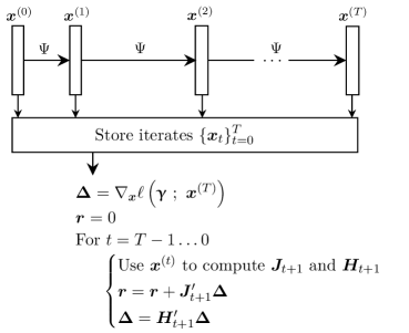
Figure B.1: Reverse mode computation of the unrolled gradient from (B.1). The first gradient computation requires ${\bm{x}}^{(T)}$, so all computations occur after the lower-level optimization algorithm is complete. The final gradient is $\nabla\ell({\bm{\upgamma}})=\nabla_{\bm{\upgamma}}\ell({\bm{\upgamma}}\,;{\bm{x}}^{(T)})+{\bm{r}}$.

Using this notation, the reverse gradient calculation of (B.1) is

$$\nabla_{\bm{\upgamma}}\ell({\bm{\upgamma}}\,;{\bm{x}}^{(T)})+\sum_{t\in[T\rightarrow 1]}{\bm{J}}_{t}{}^{\prime}\left(\prod_{s\in[(t+1)\leftarrow T]}{\bm{H}}_{s}^{\prime}\right)\nabla_{\bm{x}}\ell({\bm{\upgamma}}\,;{\bm{x}}^{(T)}).$$ (B.2)

This expression requires $\prod_{s\in[(T+1)\leftarrow T]}{\bm{H}}_{s}^{\prime}=\bm{I}$, because ${\bm{H}}_{T+1}$ is not defined. For example, for $T=3$, we have

$$\nabla_{\bm{\upgamma}}\ell({\bm{\upgamma}}\,;{\bm{x}}^{(3)})+\underbrace{{\bm{J}}_{3}^{\prime}(\bm{I}){\bm{g}}}_{t=3}+\underbrace{{\bm{J}}_{2}^{\prime}\left({\bm{H}}_{3}^{\prime}\right){\bm{g}}}_{t=2}+\underbrace{{\bm{J}}_{1}^{\prime}\left({\bm{H}}_{2}^{\prime}{\bm{H}}_{3}^{\prime}\right){\bm{g}}}_{t=1},$$

where $\bm{g}$ is shorthand for $\nabla_{\bm{x}}\ell({\bm{\upgamma}}\,;{\bm{x}}^{(T)})$ here. This version is called reverse as all computations (arrows) begin at the end, $T$.

The primary benefit of the reverse mode comes from the ability to group $\nabla_{\bm{x}}\ell({\bm{\upgamma}}\,;{\bm{x}}^{(T)})$ with the right-most ${\bm{H}}_{T}$, such that all products are matrix-vector products, as seen in Fig. B.1 Further, one can save the matrix-vector products for use during the next iteration and avoid duplicating the computation. Continuing the example for $T=3$, we have

$$\nabla_{\bm{\upgamma}}\ell({\bm{\upgamma}}\,;{\bm{x}}^{(3)})+\underbrace{{\bm{J}}_{3}^{\prime}(\bm{I}){\bm{g}}}_{t=1}+\underbrace{{\bm{J}}_{2}^{\prime}(\overbrace{{\bm{H}}_{3}^{\prime}{\bm{g}}}^{\bm{\Delta}})}_{t=2}+\underbrace{{\bm{J}}_{1}^{\prime}({\bm{H}}_{2}^{\prime}\overbrace{\left({\bm{H}}_{3}^{\prime}{\bm{g}}\right)}^{\bm{\Delta}})}_{t=3},$$

where one only needs to compute $\bm{\Delta}$ once. This ability to rearrange the parenthesis to compute matrix-vector products greatly decreases the computational requirement compared to matrix-matrix products. Excluding the costs of the optimization algorithm steps and forming the ${\bm{H}}_{s}$ and ${\bm{J}}_{t}$ matrices (these costs will be the same in the forward mode computation), reverse mode requires $\mathcal{O}\!\left(T\right)$ Hessian-vector multiplies and $\mathcal{O}\!\left(TNR\right)$ additional multiplies. The trade-off is that reverse mode requires storing all $T$ iterates, ${\bm{x}}^{(t)}$, so that one can compute the corresponding Hessians and Jacobians from them as needed, and thus has a memory complexity $\mathcal{O}\!\left(TN\right)$.

Figure B.2: Forward mode computation of the unrolled gradient from (B.3). The intermediate computation matrix, $\bm{Z}$, is initialized to zero (${\bm{Z}}_{0}=\bm{0}$) then updated every iteration. The final gradient is $\nabla\ell({\bm{\upgamma}})=\nabla_{\bm{\upgamma}}\ell({\bm{\upgamma}}\,;{\bm{x}}^{(T)})+{\bm{Z}}_{T}^{\prime}\nabla_{\bm{x}}\ell({\bm{\upgamma}}\,;{\bm{x}}^{(T)})$.

The forward mode calculation of (B.1), depicted in Fig. B.2, has all computations (arrows) starting at the earlier iterate:

$$\nabla_{\bm{\upgamma}}\ell({\bm{\upgamma}}\,;{\bm{x}}^{(T)})+\left(\sum_{t\in[1\rightarrow T]}\left(\prod_{s\in[T\leftarrow(t+1)]}{\bm{H}}_{s}\right){\bm{J}}_{t}\right)^{\prime}\nabla_{\bm{x}}\ell({\bm{\upgamma}}\,;{\bm{x}}^{(T)}).$$ (B.3)

As before, ${\bm{H}}_{T+1}$ is not defined, so we take $\prod_{s\in[T\leftarrow(T+1)]}{\bm{H}}_{s}=\bm{I}$. For example, for $T=3$ we have

$$\nabla_{\bm{\upgamma}} \ell({\bm{\upgamma}}\,;{\bm{x}}^{(T)})+\left(\underbrace{\left(({\bm{H}}_{3}{\bm{H}}_{2}){\bm{J}}_{1}\right)^{\prime}}_{t=1}+\underbrace{\left(({\bm{H}}_{3}){\bm{J}}_{2}\right)^{\prime}}_{t=2}+\underbrace{\left((\bm{I}){\bm{J}}_{3}\right)^{\prime}}_{t=3}\right){\bm{g}}.$$

How the forward mode avoids storing $\bm{x}$ iterates is evident after rearranging the parenthesis to avoid duplicate calculations, as illustrated in Fig. B.2. Continuing the example for $T=3$, we have

$$\nabla_{\bm{\upgamma}}\ell({\bm{\upgamma}}\,;{\bm{x}}^{(T)})+\left[\underbrace{{\bm{H}}_{3}\left(\overbrace{{\bm{H}}_{2}\underbrace{\left({\bm{H}}_{1}\cdot\bm{0}+{\bm{J}}_{1}\right)}_{{\bm{Z}}_{1}}+{\bm{J}}_{2}}^{{\bm{Z}}_{2}}\right)+{\bm{J}}_{3}}_{{\bm{Z}}_{3}}\right]^{\prime}{\bm{g}},$$

where ${\bm{Z}}_{s}={\bm{H}}_{s}{\bm{Z}}_{s-1}+{\bm{J}}_{s}\in\mathbb{F}^{N\times R}$ stores the intermediate calculations. The above formula also illustrates why ${\bm{H}}_{1}$ is not needed in (4.17); $\nabla_{\bm{\upgamma}}{\bm{x}}^{(0)}=\bm{0}$ is the last element from applying the chain rule.

There is no way to rearrange the terms in the forward mode formula to achieve matrix-vector products (while preserving the computation order). Therefore, the computation requirement is much higher at $\mathcal{O}\!\left(TR\right)$ Hessian-vector multiplications. The corresponding benefit of the forward mode method is that it does not require storing iterates, thus decreasing (in the common case when $T>R$) the memory requirement to $\mathcal{O}\!\left(NR\right)$ for storing the intermediate matrix ${\bm{Z}}_{s}$ during calculation.

As with the minimizer approach in Section 4.2, the computational complexity of the unrolled approach is lower than the generic bound when we consider the specific example of learning convolutional filters according to (Ex). Nevertheless, the general comparison that reverse mode takes more memory but less computation holds true. See Tab. 4.1 for a comparison of the computational and memory complexities.

Appendix C Additional Running Example Results

This appendix derives some results that are relevant to the running example used throughout the survey.

C.1 Derivatives for Convolutional Filters

This section proves the result

$$\frac{\partial}{\partial c_{{\bm{s}}}}\left(\tilde{{\bm{c}}}_{k}\circledast f.({\bm{c}}_{k}\circledast{\bm{x}})\right)=f.({\bm{c}}_{k}\circledast{\bm{z}}^{\langle{\bm{s}}\rangle})+\tilde{{\bm{c}}}_{k}\circledast\left(\dot{f}.({\bm{c}}_{k}\circledast{\bm{x}})\odot{\bm{x}}^{\langle-{\bm{s}}\rangle}\right),$$ (C.1)

when considering $\mathbb{F}=\mathbb{R}$. This equation is key to finding derivatives of the lower-level cost function in (Ex) with respect to the filter coefficients.

To simplify notation, we drop the indexing over $k$, so $\bm{c}$ is a single filter and $c_{{\bm{s}}}$ denotes the ${\bm{s}}$th element in the filter for ${\bm{s}}\in\mathbb{Z}^{D}$. Here, ${\bm{s}}$ indexes every dimension of $\bm{c}$, e.g., for a two-dimensional filter, we could equivalently write ${\bm{s}}$ as $\langle s_{1},s_{2}\rangle$. Recall that the notation $\tilde{{\bm{c}}}$ signifies a reversed version of $\bm{c}$, as needed for the adjoint of convolution.

Define the notation ${\bm{x}}^{\langle{\bm{i}}\rangle}$ as the vector $\bm{x}$ circularly shifted according to the index ${\bm{i}}$. Thus, if $\bm{x}$ is 0-indexed and we use circular indexing,

$$({\bm{x}}^{\langle{\bm{s}}\rangle})_{\bm{i}}={\bm{x}}_{{\bm{i}}-{\bm{s}}}.$$

As two examples,

$${\bm{x}}=\begin{bmatrix}x_{1}\\ x_{2}\\ \vdots\\ x_{N-1}\\ x_{N}\end{bmatrix}\rightarrow{\bm{x}}^{\langle\text{-}1\rangle}=\begin{bmatrix}x_{2}\\ x_{3}\\ \vdots\\ x_{N}\\ x_{1}\end{bmatrix},$$

and, in two dimensions, if ${\bm{X}}\in\mathbb{F}^{M\times N}$

$${\bm{X}}^{\langle 1,2\rangle}=\begin{bmatrix}x_{M,N-1}&x_{M,N}&x_{M,1}&\ldots&x_{M,3}\\ x_{1,N-1}&x_{1,N}&x_{1,1}&\ldots&x_{1,3}\\ x_{2,N-1}&x_{2,N}&x_{2,1}&\ldots&x_{2,3}\\ \vdots&&\ddots&&\vdots\\ x_{M-1,N-1}&x_{M-1,N}&x_{M-1,1}&\ldots&x_{M-1,3}\end{bmatrix}.$$

This circular shift notation is useful in the derivation and statement of the desired gradient.

Define ${\bm{z}}={\bm{c}}\circledast{\bm{x}}$, where $\bm{c}$ and $\bm{x}$ are both $N$-dimensional. By the definition of convolution, $\bm{z}$ is given by

$${\bm{z}}=\sum_{i_{1}}\cdots\sum_{i_{N}}c_{i_{1},\ldots,i_{N}}{\bm{x}}^{\langle\text{-}i_{1},\ldots,\text{-}i_{N}\rangle}\mathrel{\hbox to0.0pt{\raisebox{1.29167pt}{$\cdot$}\hss}\raisebox{-1.29167pt}{$\cdot$}}=\sum_{i_{1},\ldots,i_{N}}c_{i_{1},\ldots,i_{N}}{\bm{x}}^{\langle\text{-}{\bm{i}}\rangle},$$

where, for each sum, the indexing variable $i_{n}$ iterates over the size of $\bm{c}$ in the $i$th dimension and we simplify the index for circularly shifting vectors, $i_{1},\ldots,i_{N}$, as simply $\langle{\bm{i}}\rangle$. This expression shows that the derivative of ${\bm{c}}\circledast{\bm{x}}$ with respect to the ${\bm{s}}$th filter coefficient is the $\text{-}{\bm{s}}$th coefficient in $\bm{x}$, i.e.,

$$\frac{\partial}{\partial c_{{\bm{s}}}}({\bm{c}}\circledast{\bm{x}})={\bm{x}}^{\langle-{\bm{s}}\rangle}.$$ (C.2)

We can now find the partial derivative of interest:

$$\tilde{{\bm{c}}}\circledast f.({\bm{z}}) =\sum_{i_{1},\ldots,i_{N}}[\tilde{{\bm{c}}}]_{i_{1},\ldots,i_{N}}f.({\bm{z}})^{\langle\text{-}{\bm{i}}\rangle}$$ by the convolution formula

$$=\sum_{i_{1},\ldots,i_{N}}[\tilde{{\bm{c}}}]_{i_{1},\ldots,i_{N}}f.\left({\bm{z}}^{\langle\text{-}{\bm{i}}\rangle}\right) f$$ since operates point-wise

$$=\sum_{i_{1},\ldots,i_{N}}c_{\text{-}i_{1},\ldots,\text{-}i_{N}}f.\left({\bm{z}}^{\langle\text{-}{\bm{i}}\rangle}\right) \text{ by definition of }\tilde{{\bm{c}}}$$

$$=\sum_{i_{1},\ldots,i_{N}}c_{i_{1},\ldots,i_{N}}f.\left({\bm{z}}^{\langle{\bm{i}}\rangle}\right)$$ reverse summation order.

Recall that $\bm{z}$ is a function of $c_{{\bm{s}}}$. Therefore, using the chain rule to take the derivative,

$$\frac{\partial}{\partial c_{{\bm{s}}}} \left(\tilde{{\bm{c}}}\circledast f.({\bm{z}})\right)$$

$$=f.({\bm{z}}^{\langle s\rangle})+\sum_{i_{1}}\cdots\sum_{i_{N}}c_{i_{1},\ldots,i_{N}}\dot{f}.({\bm{z}}^{\langle i_{1},\ldots,i_{N}\rangle})\odot\nabla_{c_{{\bm{s}}}}\left({\bm{z}}^{\langle{\bm{i}}\rangle}\right)$$

$$=f.({\bm{z}}^{\langle{\bm{s}}\rangle})+\sum_{i_{1}}\cdots\sum_{i_{N}}[\tilde{{\bm{c}}}]_{\text{-}i_{1},\ldots,\text{-}i_{N}}\dot{f}.({\bm{z}}^{\langle i_{1},\ldots,i_{N}\rangle})\odot{\bm{x}}^{\langle{\bm{i}}-{\bm{s}}\rangle},$$

where the second equality follows from (C.2) and the definition of $\tilde{{\bm{c}}}$. Recognizing the convolution formula in the second summand, the expression can be simplified to

$$f.({\bm{z}}^{\langle{\bm{s}}\rangle})+\tilde{{\bm{c}}}\circledast\left(\dot{f}.({\bm{z}})\odot{\bm{x}}^{\langle-{\bm{s}}\rangle}\right).$$

This proves the claim. Note that the provided formula is for a single element in $\bm{c}$. One can concatenate the partial derivative result for each value of ${\bm{s}}$ to get the full Jacobian.

C.2 Evaluating Assumptions for the Running Example

To better understand the upper-level assumptions A$\ell$ ​1-A$\ell$ ​3 and lower-level assumptions A$\Upphi$ ​​1-A$\Upphi$ ​​6 in Section 5.3.1, this section examines whether the filter learning example (Ex) meets each assumption.

C.2.1 Upper-level Loss Assumptions

Recall the upper-level loss function in (Ex) is squared error:

$$\ell({\bm{\upgamma}}\,;\,{\bm{x}})=\dfrac{1}{2}\|{\bm{x}}-{\bm{x}}^{\text{true}}\|^{2}_{2},$$ (C.3)

where $\ell$ is typically evaluated at ${\bm{x}}={\bm{\hat{x}}}({\bm{\upgamma}})$.

The loss function (C.3) satisfies A$\ell$ ​1. Because there is no dependence on $\bm{\upgamma}$ in the upper-level, $L_{{\bm{x}},\nabla_{\bm{\upgamma}}\ell}=0$. The gradient with respect to $\bm{x}$ is $\nabla_{\bm{x}}\ell({\bm{\upgamma}}\,;\,{\bm{x}})={\bm{x}}-{\bm{x}}^{\text{true}}$, so $L_{{\bm{x}},\nabla_{\bm{x}}\ell}=1$.

The norm of the upper-level gradient with respect to $\bm{x}$,

$$\left\lVert\nabla_{\bm{x}}\ell({\bm{\upgamma}}\,;\,{\bm{x}})\right\rVert=\left\lVert{\bm{x}}-{\bm{x}}^{\text{true}}\right\rVert,$$

can grow arbitrarily large, so condition A$\ell$ ​2 is not met in general. However, in most applications, one can assume an upper bound (possibly quite large) on the elements of ${\bm{x}}^{\text{true}}$ and impose that bound as a box constraint when computing ${\bm{\hat{x}}}$. Then the triangle inequality provides a bound on $\left\lVert{\bm{x}}-{\bm{x}}^{\text{true}}\right\rVert$ for all $\bm{x}$ within the constraint box.

Finally, A$\ell$ ​3 is met by any loss function, including (C.3), that lacks cross terms between $\bm{x}$ and $\bm{\upgamma}$. We are unaware of any bilevel method papers using such cross terms.

C.2.2 Lower-level Cost Assumptions

One property used below in many of the bounds for the lower-level cost function is that

$$\sigma_{1}({\bm{C}}_{k})=\left\lVert{\bm{c}}_{k}\right\rVert_{1},$$ (C.4)

where $\sigma_{1}(\cdot)$ is a function that returns the first singular value of its matrix argument. This property follows from Young’s inequality and is related to bounded-input bounded-output stability of linear and time invariant systems [unser:05:gss].

As with the upper-level assumptions considered above, (Ex) meets the lower-level assumptions A$\Upphi$ ​​1-A$\Upphi$ ​​6 if we impose additional constraints on the maximum norm of variables. In addition to bounding the elements in $\bm{x}$, as we did to ensure A$\ell$ ​2, imposing bounds on $\left\lVert{\bm{c}}_{k}\right\rVert$ and $\lvert\beta_{k}\rvert$ is sufficient to meet all the lower-level assumptions. We now examine each condition individually.

Recall from (Ex) that the example lower-level cost function is

$${\bm{\hat{x}}}({\bm{\upgamma}}) =\operatorname*{argmin}_{{\bm{x}}\in\mathbb{F}^{N}}\dfrac{1}{2}\left\lVert{\bm{A}}{\bm{x}}-{\bm{y}}\right\rVert^{2}_{2}+e^{\beta_{0}}\sum_{k=1}^{K}e^{\beta_{k}}{\bm{1}}^{\prime}\phi.({\bm{c}}_{k}\circledast{\bm{x}};\epsilon),$$

where $\phi$ is a corner-rounded 1-norm (CR1N).

As described in Section 4.2, the minimizer approach requires $\Upphi$ to be twice differentiable. Thus, $\Upphi$ satisfies A$\Upphi$ ​​1. This condition limits the choices of $\phi$ to twice differentiable functions.

Considering A$\Upphi$ ​​2, the gradient of $\Upphi$ with respect to $\bm{x}$ is Lipschitz continuous in $\bm{x}$ if the norm of the Hessian, $\left\lVert\nabla_{{\bm{x}}{\bm{x}}}\Upphi({\bm{x}}\,;{\bm{\upgamma}})\right\rVert_{2}$, is bounded. Using (4.9) and assuming the Lipschitz constant of the derivative of $\phi$ is $L_{\dot{\phi}}$ (for (CR1N), $L_{\dot{\phi}}=\tfrac{1}{\epsilon}$), a Lipschitz constant for $\nabla_{\bm{x}}\Upphi$ is

$$L_{{\bm{x}},\nabla_{\bm{x}}\Upphi} =\sigma_{1}^{2}({\bm{A}})+L_{\dot{\phi}}e^{\beta_{0}}\sum_{k}e^{\beta_{k}}\sigma_{1}({\bm{C}}_{k}^{\prime}{\bm{C}}_{k})$$

$$=\sigma_{1}^{2}({\bm{A}})+L_{\dot{\phi}}e^{\beta_{0}}\sum_{k}e^{\beta_{k}}\left\lVert{\bm{c}}_{k}\right\rVert_{1}^{2}\text{ by \eqref{eq: sigma1 Ck}}.$$ (C.5)

The Lipschitz constant $L_{{\bm{x}},\nabla_{\bm{x}}\Upphi}$ depends on the values in $\bm{\upgamma}$ and therefore does not strictly satisfy A$\Upphi$ ​​2. Here if $\beta_{0}$, $\beta_{k}$, and ${\bm{c}}_{k}$ have upper bounds, then one can upper bound $L_{{\bm{x}},\nabla_{\bm{x}}\Upphi}$. All of the bounds below have similar considerations.

To consider the strong convexity condition in A$\Upphi$ ​​3, we consider the Hessian,

$$\nabla_{{\bm{x}}{\bm{x}}}\Upphi({\bm{x}}\,;{\bm{\upgamma}})=\underbrace{{\bm{A}}^{\prime}{\bm{A}}}_{\text{From data-\\ fit term}}+\underbrace{e^{\beta_{0}}\sum_{k}e^{\beta_{k}}{\bm{C}}_{k}^{\prime}\text{diag}({\ddot{\phi}}.({\bm{c}}_{k}\circledast{\bm{x}})){\bm{C}}_{k}}_{\text{From regularizer}}.$$ (C.6)

We assume that ${\ddot{\phi}}(z)\geq 0\,\forall z$, as is the case for the corner rounded 1-norm. If ${\bm{A}}^{\prime}{\bm{A}}$ is positive-definite with $\sigma_{N}({\bm{A}}^{\prime}{\bm{A}})>0$ (this is equivalent to $\bm{A}$ having full column rank), then the Hessian is positive-definite and $\mu_{{\bm{x}},\Upphi}=\sigma_{N}^{2}({\bm{A}})$ suffices as a strong convexity parameter. In applications like compressed sensing, $\bm{A}$ does not have full column rank. In such cases, $\sigma_{N}({\bm{A}}^{\prime}{\bm{A}})=0$ and as $e^{\beta_{0}}\rightarrow 0$ the regularizer term vanishes, so there does not exist any universal $\mu_{{\bm{x}},\Upphi}>0$ for all ${\bm{\upgamma}}\in\mathbb{F}^{R}$, so the strong convexity condition A$\Upphi$ ​​3 is not satisfied. However, as discussed in Section 4.2.3, the condition may hold in practice for many values of $\bm{\upgamma}$. How to adapt the complexity theory to rigorously address these subtleties is an open question.

The fourth condition, A$\Upphi$ ​​4, is that $\nabla_{{\bm{x}}{\bm{x}}}\Upphi({\bm{x}}\,;{\bm{\upgamma}})$ and $\nabla_{{\bm{\upgamma}}{\bm{x}}}\Upphi({\bm{x}}\,;{\bm{\upgamma}})$ are Lipschitz continuous with respect to $\bm{x}$ for all $\bm{\upgamma}$. For the first part part, a Lipschitz constant results from bounding the difference in the Hessian evaluated at two points, ${\bm{x}}^{(1)}$ and ${\bm{x}}^{(2)}$:

$$\left\lVert\nabla_{{\bm{x}}{\bm{x}}}\Upphi({\bm{x}}^{(1)}\,;{\bm{\upgamma}})-\nabla_{{\bm{x}}{\bm{x}}}\Upphi({\bm{x}}^{(2)}\,;{\bm{\upgamma}})\right\rVert_{2}$$

$$\quad\quad=\left\lVert e^{\beta_{0}}\sum_{k}e^{\beta_{k}}{\bm{C}}_{k}^{\prime}\text{diag}({\ddot{\phi}}.({\bm{c}}_{k}\circledast{\bm{x}}^{(1)})-{\ddot{\phi}}({\bm{c}}_{k}\circledast{\bm{x}}^{(2)})){\bm{C}}_{k}\right\rVert_{2}.$$

Since every element of $\ddot{\phi}$is bounded in $(0,L_{\dot{\phi}})$, the difference between any two evaluations of $\ddot{\phi}$is at most $L_{\dot{\phi}}$. Thus

$$\left\lVert\nabla_{{\bm{x}}{\bm{x}}}\Upphi({\bm{x}}^{(1)}\,;{\bm{\upgamma}})-\nabla_{{\bm{x}}{\bm{x}}}\Upphi({\bm{x}}^{(2)}\,;{\bm{\upgamma}})\right\rVert_{2} \leq e^{\beta_{0}}L_{\dot{\phi}}\sum_{k}e^{\beta_{k}}\left\lVert{\bm{C}}_{k}^{\prime}{\bm{C}}_{k}\right\rVert_{2}$$

$$\leq e^{\beta_{0}}L_{\dot{\phi}}\sum_{k}e^{\beta_{k}}\left\lVert{\bm{c}}_{k}\right\rVert^{2}_{1}.$$

The final simplification again uses (C.4). Thus,

$$L_{{\bm{x}},\nabla_{{\bm{x}}{\bm{x}}}\Upphi}=e^{\beta_{0}}L_{\dot{\phi}}\sum_{k}e^{\beta_{k}}\left\lVert{\bm{c}}_{k}\right\rVert^{2}_{1}.$$

For the second part of A$\Upphi$ ​​4, we must look at the tuning parameters and filter coefficients separately. When considering learning a tuning parameter, $\beta_{k}$,

$$\nabla_{\beta_{k}{\bm{x}}}\Upphi({\bm{x}}\,;{\bm{\upgamma}}) =e^{\beta_{0}+\beta_{k}}{\bm{C}}_{k}^{\prime}{{\dot{\phi}}}.({\bm{C}}_{k}{\bm{x}}).$$

To find a Lipschitz constant, consider the Jacobian:

$$\nabla_{\bm{x}}\left(\nabla_{\beta_{k}{\bm{x}}}\Upphi({\bm{x}}\,;{\bm{\upgamma}})\right) =e^{\beta_{0}+\beta_{k}}{\bm{C}}_{k}^{\prime}\text{diag}({\ddot{\phi}}.({\bm{C}}_{k}{\bm{x}})){\bm{C}}_{k}.$$

A Lipschitz constant of $\nabla_{\beta_{k}{\bm{x}}}\Upphi({\bm{x}}\,;{\bm{\upgamma}})$ is given by the bound on the norm of this matrix (we chose to use the matrix 2-norm, also called the spectral norm). Using similar steps as above to simplify the expression, $L_{{\bm{x}},\nabla_{\beta_{k}{\bm{x}}}\Upphi}=e^{\beta_{0}+\beta_{k}}L_{\dot{\phi}}\left\lVert{\bm{c}}_{k}\right\rVert^{2}_{1}$.

When considering learning the ${\bm{s}}$th element of the $k$th filter,

$$\nabla_{c_{k,{\bm{s}}}{\bm{x}}}\Upphi({\bm{x}}\,;{\bm{\upgamma}}) =e^{\beta_{0}+\beta_{k}}\left({{\dot{\phi}}}.(({\bm{C}}_{k}{\bm{x}})^{\langle s\rangle})+{\bm{C}}_{k}^{\prime}\left({\ddot{\phi}}.({\bm{C}}_{k}{\bm{x}})\odot{\bm{x}}^{\langle\text{-}s\rangle}\right)\right)$$

$$=e^{\beta_{0}+\beta_{k}}\left(\underbrace{{{\dot{\phi}}}.({\bm{R}}_{1}{\bm{C}}_{k}{\bm{x}})}_{\text{Expression 1}}+\underbrace{{\bm{C}}_{k}^{\prime}\left({\ddot{\phi}}.({\bm{C}}_{k}{\bm{x}})\odot{\bm{R}}_{2}{\bm{x}}\right)}_{\text{Expressions 2-3}}\right)\in\mathbb{F}^{N},$$

where ${\bm{R}}_{1}$ and ${\bm{R}}_{2}$ are rotation matrices that depends on ${\bm{s}}$ such that ${\bm{R}}_{1}{\bm{x}}={\bm{x}}^{\langle{\bm{s}}\rangle}$ and ${\bm{R}}_{2}{\bm{x}}={\bm{x}}^{\langle\text{-}{\bm{s}}\rangle}$. For taking the gradient, it is convenient to note that the last term can be expressed in multiple ways:

$${\ddot{\phi}}.({\bm{C}}_{k}{\bm{x}})\odot{\bm{x}}^{\langle\text{-}{\bm{s}}\rangle}=\underbrace{\text{diag}({\ddot{\phi}}.({\bm{C}}_{k}{\bm{x}})){\bm{R}}_{2}{\bm{x}}}_{\mathrm{Expression\,2}}=\underbrace{\text{diag}({\bm{R}}_{2}{\bm{x}}){\ddot{\phi}}.({\bm{C}}_{k}{\bm{x}})}_{\mathrm{Expression\,3}}.$$

Using the alternate expressions to perform the chain rule with respect to the $\bm{x}$ term that is not in the $\text{diag}(\cdot)$ statement, the gradient with respect to $\bm{x}$ is:

$$\nabla_{\bm{x}}\left(\nabla_{c_{k,s}{\bm{x}}}\Upphi({\bm{x}}\,;{\bm{\upgamma}})\right)=e^{\beta_{0}+\beta_{k}}( \underbrace{{\bm{C}}_{k}^{\prime}{\bm{R}}_{1}^{\prime}\text{diag}({\ddot{\phi}}.({\bm{R}}_{1}{\bm{C}}_{k}{\bm{x}}))}_{\mathrm{Expression\,1}}$$

$$+\underbrace{{\bm{C}}_{k}^{\prime}\text{diag}({\ddot{\phi}}.({\bm{C}}_{k}{\bm{x}})){\bm{R}}_{2}}_{\mathrm{Expression\,2}}$$

$$+\underbrace{{\bm{C}}_{k}^{\prime}\text{diag}(\dddot{\phi}({\bm{C}}_{k}{\bm{x}}))\text{diag}({\bm{R}}_{2}{\bm{x}})^{\prime}{\bm{C}}_{k}}_{\mathrm{Expression\,3}}).$$

The bound on the spectral norm of the first and second expressions are both $\sigma_{1}({\bm{C}}_{k})L_{\dot{\phi}}$ because, for any ${\bm{z}}\in\mathbb{F}^{N}$,

$$\|\text{diag}({\ddot{\phi}}.({\bm{z}}))\|_{2}\leq\operatorname*{max}_{z}\lvert{\ddot{\phi}}(z)\rvert=L_{\dot{\phi}}.$$

The third expression is bounded by $\sigma_{1}^{2}({\bm{C}}_{k})\left\lVert{\bm{x}}\right\rVert_{2}L_{\ddot{\phi}}$, which requires a bound on the norm of $\bm{x}$, similar to A$\ell$ ​2. Summing the three expressions and including the tuning parameters gives the final Lipschitz constant

$$L_{{\bm{x}},\nabla_{c_{k,s}{\bm{x}}}\Upphi}=e^{\beta_{0}+\beta_{k}}\sigma_{1}({\bm{C}}_{k})(2L_{\dot{\phi}}+\sigma_{1}({\bm{C}}_{k})L_{\ddot{\phi}}\left\lVert{\bm{x}}\right\rVert_{2}).$$ (C.7)

The fifth assumption, A$\Upphi$ ​​5 states that the mixed second gradient of $\Upphi$ is bounded. For the tuning parameters, the mixed second gradient is given in (4.9) as

$$\nabla_{\beta_{k}{\bm{x}}}\Upphi({\bm{\hat{x}}}\,;{\bm{\upgamma}})=e^{\beta_{0}}e^{\beta_{k}}\tilde{{\bm{c}}}_{k}\circledast{{\dot{\phi}}}.({\bm{c}}_{k}\circledast{\bm{\hat{x}}}).$$

The bound given in A$\Upphi$ ​​5 follows easily by considering that

$$\|\text{diag}({{\dot{\phi}}}.({\bm{c}}_{k}\circledast{\bm{\hat{x}}}))\|_{2}\leq\operatorname*{max}_{z}\lvert{{\dot{\phi}}}(z)\rvert=L_{\phi}.$$

For a filter coefficient, the mixed second gradient is more complicated:

$$\nabla_{c_{k,{\bm{s}}}{\bm{x}}}\Upphi({\bm{\hat{x}}}\,;{\bm{\upgamma}})=e^{\beta_{0}+\beta_{k}}\Big{(}\underbrace{{{\dot{\phi}}}.(({\bm{c}}_{k}\circledast{\bm{\hat{x}}})^{\langle{\bm{s}}\rangle})}_{\text{Bounded by $L_{\phi}$}}+\tilde{{\bm{c}}}_{k}\circledast\Big{(}\underbrace{{\ddot{\phi}}.({\bm{c}}_{k}\circledast{\bm{\hat{x}}})}_{\text{Bounded by $L_{\dot{\phi}}$}}\odot{\bm{\hat{x}}}^{\langle\text{-}{\bm{s}}\rangle}\Big{)}\Big{)}.$$

Assuming that the bounds $L_{\phi}$ and $L_{\dot{\phi}}$ exist (they are $1$ and $\frac{1}{\epsilon}$ respectively for (CR1N)), a bound on the norm of the mixed gradient is

$$\|\nabla_{c_{k,{\bm{s}}}{\bm{x}}}\Upphi({\bm{\hat{x}}}\,;{\bm{\upgamma}})\|_{2} \leq e^{\beta_{0}+\beta_{k}}\left(L_{\phi}+L_{\dot{\phi}}\left\lVert{\bm{c}}_{k}\right\rVert_{1}\left\lVert{\bm{x}}\right\rVert_{2}\right).$$

The sixth assumption, A$\Upphi$ ​​6, is that $L_{{\bm{\upgamma}},\nabla_{{\bm{\upgamma}}{\bm{x}}}\Upphi}$ and $L_{{\bm{\upgamma}},\nabla_{{\bm{x}}{\bm{x}}}\Upphi}$ exist. Lipschitz constants for the tuning parameters are

$$L_{\beta_{k},\nabla_{\beta_{k}{\bm{x}}}\Upphi}=e^{\beta_{0}+\beta_{k}}\left\lVert{\bm{c}}_{k}\right\rVert_{1}L_{\phi}\text{ and }L_{\beta_{k},\nabla_{{\bm{x}}{\bm{x}}}\Upphi}=e^{\beta_{0}+\beta_{k}}\left\lVert{\bm{c}}_{k}\right\rVert^{2}_{1}L_{\dot{\phi}}.$$

Using similar derivations as shown above, corresponding Lipschitz constants for the filter coefficients are

$$L_{c_{k,s},\nabla_{c_{k,s}{\bm{x}}}\Upphi} =e^{\beta_{0}+\beta_{k}}\left(L_{\phi}+\left\lVert{\bm{x}}\right\rVert_{2}\left(L_{\dot{\phi}}+L_{\ddot{\phi}}\left\lVert{\bm{c}}_{k}\right\rVert_{1}\left\lVert{\bm{x}}\right\rVert_{2}\right)\right)$$

$$L_{c_{k,s},\nabla_{{\bm{x}}{\bm{x}}}\Upphi} =e^{\beta_{0}+\beta_{k}}\left(2L_{\dot{\phi}}\left\lVert{\bm{c}}_{k}\right\rVert_{1}+L_{\ddot{\phi}}\left\lVert{\bm{c}}_{k}\right\rVert_{1}^{2}\left\lVert{\bm{x}}\right\rVert_{2}\right).$$

This is the last lower-level condition in Section 5.3.1 for the single-loop and double-loop bilevel optimization method analysis.

Appendix D Implementation Details

This appendix describes the experimental settings used throughout this review. We first present the common settings; the following sub-sections detail any differences specifically for the results in Fig. 1.3 and for the series of figures using the cameraman image (Fig. 5.2, Fig. 6.1, and Fig. 6.2). The code for all experiments is available on github [crockett:2022:bilevelfilterlearningforimagerecon].

The experiments consider the denoising problem (${\bm{A}}=\bm{I}$) and use (CR1N) as the sparsifying function $\phi$ with $\epsilon=0.01$. The training data is typically on the scale $[0,\,1]$ and noisy samples are generated from the clean training data using (1.4) with zero-mean Gaussian noise with a standard deviation of $\sigma=25/255$, following [chen:2014:insightsanalysisoperator].

The lower-level optimizer is the optimized gradient method (OGM) with gradient-based restart [kim:18:aro]. We calculate the step-size based on the Lipschitz constant of the lower-level gradient using (C.5) every upper-level iteration. Each experiment sets a maximum number of lower-level iterations, but the lower-level optimization will terminate early if it converges, defined as if $\left\lVert\nabla_{{\bm{x}}}\Upphi({\bm{x}}\,;{\bm{\upgamma}})\right\rVert<10^{\text{-}5}$.

The upper-level optimizer follows the general structure of the double-loop procedure outlined in Alg. 3. To compute $\nabla\ell({\bm{\upgamma}})$, we use the minimizer formulation (4.8), with the conjugate gradient (CG) method to compute the Hessian-inverse-vector product (4.10). As suggested in [ji:2021:bileveloptimizationconvergence], the initialization for the lower-level optimization is the estimated minimizer from the previous outer loop iteration, ${\bm{x}}^{(T)}({{\bm{\upgamma}}^{(u\text{-}1)}})$ and the initialization for the CG method is the solution from the previous CG iteration. Following [chen:2021:learnabledescentalgorithm] and other bilevel works, the experiments use Adam with the default parameters [kingma:2015:adammethodstochastic] to determine the size of the upper-level gradient descent; this choice avoids introducing the tuning parameter $\alpha_{\ell}$.

The learnable parameters include the filter coefficients and the tuning parameters $\beta_{k}$ for $k\in[1,K]$. The experiments either use random or DCT filters to initialize $\bm{h}$. An initial grid search determines the tuning parameter $\beta_{0}$; $\beta_{k}$ for $k\in[1,K]$ are initialized as 0 such that $e^{\beta_{k}}=1$.

D.1 Vertical Bar Training Image

This section describes additional details for Fig. 1.3. This simple proof of concept used 50 lower-level iterations ($T=50$) and 4,000 upper-level iterations ($U=4,000$). The initial grid search for $\beta_{0}$ yielded $\text{-}4.6$.

When $\phi(z)=\lvert z\rvert$, one can absorb the $k$th filter’s magnitude into the tuning parameter $\beta_{k}$ because $\left\lVert{\bm{c}}_{k}\circledast{\bm{x}}\right\rVert_{1}=\left\lVert{\bm{c}}_{k}\right\rVert_{2}\left\lVert\frac{1}{\left\lVert{\bm{c}}_{k}\right\rVert_{2}}{\bm{c}}_{k}\circledast{\bm{x}}\right\rVert_{1}$. When using (CR1N), this equality no longer holds, but

$$e^{\beta_{0}+\beta_{k}}\left\lVert{\bm{c}}_{k}\right\rVert_{2}$$ (D.1)

still provides a reasonable approximation for the overall regularization strength for the $k$th filter. From left to right, the approximate regularization strengths of the filters in Fig. 1.3 are 0.77, 0.49, 0.17, and 0.05.

The learned filters reflect that the training data is constant along the columns. Visually, the filters resemble vertical (extended) finite differences. This matches our expectations as a filter that takes vertical finite differences will exactly sparsify the noiseless signal. Further, the maximum sum of the columns of the learned filters is $10^{\text{-}5}$. In contrast, the sum of the rows of the learned filters varies from $\text{-}2.6$ to 3.0.

D.2 Cameraman Training Image

This section describes the experimental settings for Fig. 5.2, Fig. 6.2, and Fig. 6.1.

To reduce computation, we selected three $50\times 50$ patches from the “cameraman” image in Fig. 6.2 to use as the training data. We hand selected the training patches to contain structure. Fig. D.1 shows the training image patches.

We set the lower-level initialization ${\bm{\hat{x}}}({\bm{\upgamma}}^{(0)})$ by optimizing the lower-level cost function until the norm of the gradient fell below a threshold for each training patch, i.e., until $\tfrac{1}{\sqrt{N}}\left\lVert\nabla_{\bm{x}}\Upphi\left({\bm{\hat{x}}}_{j}({\bm{\upgamma}}^{(0)})\,;\,{\bm{\upgamma}}^{(0)}\right)\right\rVert_{2}<10^{\text{-}7}$ for $j\in[1,J]$. The lower-level optimizer consisted of 10 iterations of OGM [kim:18:aro].

As shown in Fig. 6.1, the initial filters are the 48 non-constant DCT filters of size $7\times 7$. The initial grid search for $\beta_{0}$ yielded $\text{-}4$. In summary, the settings are $J=3$, $N=50\cdot 50$, $S=7\cdot 7$, $K=48$, $R=48(49+1)=2400$, $\beta_{0}=\text{-}4$, $T=10$, and $U=10,000$.

Fig. 6.1 shows the learned filters. To visualize the filters when $\bm{\upgamma}$ includes $\bm{h}$, Fig. 6.1c scales each learned filter $\hat{{\bm{c}}}_{k}$ to have unit norm. Fig. D.2 shows the learned filters with the effective regularization strength printed above each filter.

Figure D.1: Patches from the cameraman test images used as the training dataset.

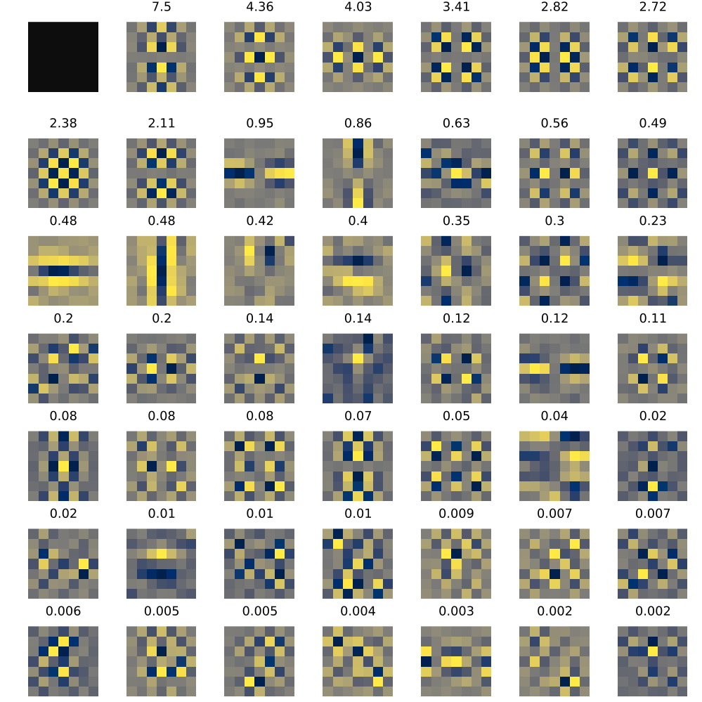
Figure D.2: Learned filers for (Ex) when $\bm{\upgamma}$ includes $\bm{h}$ and $\bm{\beta}$, ordered by their effective regularization strength $e^{\beta_{k}}\left\lVert{\bm{c}}_{k}\right\rVert_{2}$, which is printed above each filter. This effective regularization does not include the influence of $e^{\beta_{0}}$, which is uniform across all filters.