Higher mass limits of neutron stars from the equation of states in curved spacetime

Abstract

In order to solve the Tolman-Oppenheimer-Volkoff equations for neutron stars, one routinely uses the equation of states which are computed in the Minkowski spacetime. Using a first-principle approach, it is shown that the equation of states which are computed within the curved spacetime of the neutron stars include the effect of gravitational time dilation. It arises due to the radially varying interior metric over the length scale of the star and consequently it leads to a much higher mass limit. As an example, for a given set of parameters in a $\sigma-\omega$ model of nuclear matter, the maximum mass limit is shown to increase from $1.61M_{\odot}$ to $2.24M_{\odot}$ due to the inclusion of gravitational time dilation.

I Introduction

A key lesson of Einstein’s general relativity is that a curved spacetime can be described locally by the Minkowski metric i.e. a curved spacetime is locally flat. This argument is then often used to deploy the equation of states which are computed in the Minkowski spacetime, for solving the Tolman-Oppenheimer-Volkoff (TOV) equations in the study of neutron stars. Here we refer such an equation of state (EOS) as a flat EOS. It may be noted that the TOV eqs. follow from Einstein’s equation for a spherically symmetric interior geometry in the general relativity.

However, such an approach overlooks the fact that two locally inertial frames which are located at different radial positions within the star, are not identical as these frames are subject to the gravitational time dilation. In other words, while the spacetime metric of these two frames are locally flat, the corresponding clock rates are not the same as they have different lapse functions. This aspect directly impacts the respective matter field dynamics. After all, as famously stated by Wheeler, in general relativity not only matter tells spacetime how to curve but also spacetime tells matter how to move.

Recently, by employing a first-principle approach, we gave a derivation of the equation of state for an ensemble of non-interacting degenerate neutrons in the interior curved spacetime of a spherical star Hossain and Mandal (2021). We refer such an equation of state as a curved EOS. For regular stars the effect of gravitational time dilation on their matter field dynamics is negligible. However, for the compact stars, such as the neutron stars, the effect of gravitational time dilation is significant. In particular, we have shown in the ref. Hossain and Mandal (2021) that for a neutron star containing non-interacting ideal degenerate neutrons, the maximum mass limit increases from $0.71M_{\odot}$ to $0.83M_{\odot}$. Clearly, the usage of flat EOS leads one to underestimate the maximum mass limit.

Nevertheless, the consideration of non-interacting degenerate neutron matter alone is not sufficient to describe the matter contents of the astrophysical neutron stars whose maximum mass limits have now been observed to be more than $2M_{\odot}$ Shapiro and Teukolsky (2008); Nättilä et al. (2017); Özel et al. (2016). In order to explain the observed mass-radius relation of the neutron stars, various kinds of nuclear matter EOS have been studied in the literature Shen (2002); Lattimer and Prakash (2016); Douchin and Haensel (2001); Tolos et al. (2016); Maieron et al. (2004); Klähn et al. (2007); Baldo et al. (2007). These models are inspired by different particle physics models and generally include different types of interactions between the possible nucleons for describing the nuclear matter contained within the astrophysical neutron stars. Among them, a widely used model is known as the so-called $\sigma-\omega$ model Whittenbury et al. (2014); Katayama et al. (2012); Miyatsu et al. (2013) that includes interacting baryons, leptons, mesons, and often a set of hyperons Chatterjee and Vidana (2016); Schaffner-Bielich (2008); Balberg et al. (1999); Dhapo et al. (2010); Bednarek and Manka (2001); Hornick et al. (2018).

In order to perform a first-principle derivation of the equation of states using interior curved spacetime of the neutron stars, here we consider a simplified $\sigma-\omega$ model containing the neutron, the proton and the electron as the fermions and a scalar meson $\sigma$ and a self-interacting vector meson $\omega$. Subsequently, we show that the EOS which is derived in the curved spacetime, incorporates the effect of gravitational time dilation. The EOS reduces exactly to its flat spacetime counterpart when the effect of time dilation is turned-off. By considering different sets of parameters, we show that the maximum mass limits of the neutron stars always increase due to the inclusion of general relativistic time dilation.

This article is organized as follows. In the section II, we briefly review the form of the spherically symmetric interior metric of the stars. In the section III, we study the $\sigma-\omega$ model in detail. In particular, by computing the grand canonical partition function, we derive the equation of state corresponding to the $\sigma-\omega$ model by using the interior curved spacetime. In the section IV, by employing numerical methods, we study the properties of the curved EOS and then compare it with the corresponding flat EOS. Subsequently, we solve the TOV eqs. numerically to obtain the mass-radius relations of the neutron stars. In the section V, we discuss about the general transformations that are required to obtain the curved EOS starting from the corresponding flat EOS. We conclude the article with the discussions in the section VI.

II Interior metric of spherical stars

The invariant distance element inside a spherically symmetric star can be expressed as

$$ds^{2}=-e^{2\Phi(r)}dt^{2}+e^{2\nu(r)}dr^{2}+r^{2}(d\theta^{2}+\sin^{2}\theta d\phi^{2})~{},$$ (1)

where we have used the so-called natural units i.e. the speed of light $c$ and Plank’s constant $\hbar$ are set to unity. In general relativity, the metric functions $\Phi(r)$ and $\nu(r)$ are governed by Einstein’s equation and the conservation equation of the stress-energy tensor. These equations, known as the TOV equations, are given by

$$\frac{d\Phi}{dr}=\frac{G(\mathcal{M}+4\pi r^{3}P)}{r(r-2G\mathcal{M})}~{}~{},~{}~{}\frac{dP}{dr}=-(\rho+P)\frac{d\Phi}{dr}~{},$$ (2)

where $d\mathcal{M}=4\pi r^{2}\rho dr$, $P$ is the pressure and $\rho$ is the energy density. Additionally, the equation for the metric function $\nu(r)$ can be partially solved to obtain a relation $e^{-2\nu(r)}=(1-2G\mathcal{M}/r)$.

III $\sigma-\omega$ model of nuclear matter

In the framework of quantum hadrodynamics (QHD) Serot (1992); Serot and Walecka (1997), the $\sigma-\omega$ model is a well-known model which is often used to describe the nuclear matter contained within the neutron stars. In order to study the effect of gravitational time dilation on the properties of the equation of states, here we consider a simplified $\sigma-\omega$ model containing two baryons, namely the neutron and the proton, a lepton namely the electron, a massive scalar meson $\sigma$ and a self-interacting vector meson $\omega$. The corresponding action in an arbitrary curved spacetime with a metric $g_{\mu\nu}$ can be expressed as

$$S=\int d^{4}x\sqrt{-g}~{}\mathcal{L}=\int d^{4}x\sqrt{-g}\left[\mathcal{L}_{D}+\mathcal{L}_{M}\right]~{},$$ (3)

where $g$ is the metric determinant. The Lagrangian density for the Dirac fermions is

$$\mathcal{L}_{D}=-\sum_{I=n,p,e}\bar{\psi}_{I}(i{e^{\mu}}_{a}\gamma^{a}\mathcal{D}_{\mu}+m_{I})\psi_{I}~{},$$ (4)

where ${e^{\mu}}_{a}$ are the tetrad components and $\mathcal{D}_{\mu}$ is the covariant derivative of the spinor fields Hossain and Mandal (2021). The indices $n$, $p$ and $e$ refer to the neutron, the proton and the electron respectively. Here Dirac matrices $\gamma^{a}$ satisfy $\{\gamma^{a},\gamma^{b}\}=-2\eta^{ab}\mathbb{I}$ with $\eta^{ab}$ being the Minkowski metric. The total Lagrangian density for the mesons $\sigma$ and $\omega$ can be expressed as $\mathcal{L}_{M}=\mathcal{L}_{\sigma}+\mathcal{L}_{\sigma i}+\mathcal{L}_{\omega}+\mathcal{L}_{\omega i}$, where the Lagrangian density for the free $\sigma$ meson is

$$\mathcal{L}_{\sigma}=-\frac{1}{2}g^{\mu\nu}\partial_{\mu}\sigma\partial_{\nu}\sigma-\frac{1}{2}m_{\sigma}^{2}\sigma^{2}~{},$$ (5)

and its interaction with the baryons is described by

$$\mathcal{L}_{\sigma i}=\sum_{I=n,p}g_{\sigma}\sigma\,\bar{\psi}_{I}\psi_{I}~{},$$ (6)

with $g_{\sigma}$ being the dimensionless coupling constant. Similarly, the Lagrangian density for the free vector meson $\omega$ is given by

$$\mathcal{L}_{\omega}=-g^{\mu\rho}g^{\nu\lambda}(\nabla_{[\mu}\omega_{\nu]})(\nabla_{[\rho}\omega_{\lambda]})-\frac{1}{2}m_{\omega}^{2}g^{\mu\nu}\omega_{\mu}\omega_{\nu}~{},$$ (7)

where $\nabla_{[\mu}\omega_{\nu]}=\tfrac{1}{2}(\nabla_{\mu}\omega_{\nu}-\nabla_{\nu}\omega_{\mu})$. The self-interaction of $\omega$ meson and its interaction with the baryons are described by

$$\mathcal{L}_{\omega i}=\frac{\zeta~{}g_{\omega}^{4}}{4!}(g^{\mu\nu}\omega_{\mu}\omega_{\nu})^{2}+\sum_{I=n,p}g_{\omega}\omega_{\mu}{e^{\mu}}_{a}\bar{\psi}_{I}\gamma^{a}\psi_{I}~{},$$ (8)

where $g_{\omega}$ is the coupling constant with the baryons and $\zeta$ is the coupling constant controlling its quartic self-interaction. Both of these coupling constants here are dimensionless.

III.1 Reduced action for fermions

Inside a star, the pressure $P$ and the energy density $\rho$ both vary radially. On the other hand, at a thermodynamical equilibrium, these quantities are required to be uniform within the system of interest. In order to reconcile these two apparently conflicting aspects, one needs to consider a sufficiently small spatial region around every given point such that the physical quantities within the small region can be considered to be spatially uniform. At the same, the small region must also contain sufficiently large number of degrees of freedom for achieving the thermal equilibrium. In other words, around every point inside the star the notion of a local thermodynamical equilibrium must hold.

We have mentioned earlier that one can always find a locally flat coordinate system around any given point. Here we follow the ref. Hossain and Mandal (2021), to construct such a locally flat coordinate system which also retains the information about the corresponding lapse function. Let us consider a small box around a point which is located at a radial location $r_{0}$. In order to achieve a local thermodynamical equilibrium, the metric functions $\Phi(r)$ and $\nu(r)$ within the box can be approximated to be uniform. For a spherical star we can always rotate the polar axis such that it passes through the center of the box. It ensures $\theta$ to be small for every points within the box. Subsequently, by defining a new set of coordinates $X=e^{\nu(r_{0})}r\sin\bar{\theta}\cos\phi$, $Y=e^{\nu(r_{0})}r\sin\bar{\theta}\sin\phi$, and $Z=e^{\nu(r_{0})}r\cos\bar{\theta}$ along with $\bar{\theta}=e^{-\nu(r_{0})}\theta$, one can reduce the metric inside the box to be

$$ds^{2}=-e^{2\Phi(r_{0})}dt^{2}+dX^{2}+dY^{2}+dZ^{2}~{}.$$ (9)

We note that the metric (9) despite being flat within the box, is not globally flat as the radial location of the box in the metric function $\Phi(r_{0})$ is retained. In other words, for the purpose of computing the equation of states of the nuclear matter within the box, $\Phi(r_{0})$ has a fixed value whereas in the TOV eqs. (2) the same metric function can be seen to be varying radially, as like the pressure $P(r_{0})$ and the energy density $\rho(r_{0})$ within the box.

By assuming a diagonal form, the tetrad and the inverse tetrad corresponding to the metric (9), can be written as

$${e_{\mu}}^{a}=diag(e^{\Phi},1,1,1)~{},~{}{e^{\mu}}_{a}=diag(e^{-\Phi},1,1,1)~{},$$ (10)

where $\Phi\equiv\Phi(r_{0})$. As a consequence, the associated spin-connections of the spin-covariant derivative $\mathcal{D}_{\mu}$ or equivalently Ricci rotation coefficients Dvornikov (2019) of the tetrad fields vanish and the spin-covariant derivative becomes $\mathcal{D}_{\mu}=\partial_{\mu}$. The diagonal ansatz for the tetrad (10) fixes the gauge freedoms that arise due to the usage tetrad field. In general, the tetrad field in 4 dimension has 16 components at each spacetime point in contrast to the metric field which has only 10 components. The Dirac action describing the free fermions, then reduces to

$$S_{D}=-\int d^{4}x\sum_{I}\bar{\psi}_{I}\left[i\gamma^{0}\partial_{0}+e^{\Phi}\left(i\gamma^{k}\partial_{k}+m_{I}\right)\right]\psi_{I}~{},$$ (11)

where the index $k$ runs over $1,2,3$. The conserved charge, corresponding to the 4-current $j^{\mu}_{I}$ of the $I^{\text{th}}$ fermion, then becomes $Q_{I}=\int d^{3}x\sqrt{-g}j^{0}_{I}=\int d^{3}x\bar{\psi}_{I}\gamma^{0}\psi_{I}$.

The reduced action (11) within the box can be viewed as a modified spinor action written in the Minkowski spacetime with metric $diag(-1,1,1,1)$. It contains the information about the global metric function $\Phi$, unlike the spinor action which is written in a globally flat spacetime and routinely used in the literature. We employ this modified spinor action for subsequent analysis.

III.2 RMF approximation for mesons

In QHD, the coupling strengths of interactions are not necessarily weak. In other words, a potential perturbation series will diverge unless an appropriate resummation method Andersen and Strickland (2005); Sterman and Tejeda-Yeomans (2003) is applied but application of such a method is often not feasible. Further, any approximation method that one employs is required to be accurate for both lower and higher baryon number densities. In this context, such aims are usually achieved by using the so-called relativistic mean field (RMF) approximation Ring (1996); Mueller and Serot (1996).

In the RMF approximation, one replaces the meson field operators by their vacuum expectation values which are then treated as the classical fields. On the other hand, the vacuum expectation values of the kinetic terms and the spatial components $\langle\hat{\omega}^{i}\rangle\equiv\bra{0}\hat{\omega}^{i}\ket{0}$ vanish as these expectation values within the box should be both uniform and stationary to ensure local thermodynamical equilibrium. In summary, for the meson fields, the RMF approximation leads to

$$\hat{\omega}^{\mu}\rightarrow\langle\hat{\omega}^{\mu}\rangle=\langle\hat{\omega}^{0}\rangle\delta_{0}^{\mu}=\langle\hat{\omega}_{0}\rangle g^{0\mu}~{}~{},~{}~{}\hat{\sigma}\rightarrow\langle\hat{\sigma}\rangle~{}.$$ (12)

In principle, the coupling constants $g_{\sigma}$ and $g_{\omega}$ can have different values for different baryons. However, for simplicity here we assume that these coupling constants have same values for both neutrons and protons. The Euler-Lagrange equation for the $\sigma$ meson then becomes

$$\bar{\sigma}\equiv m_{\sigma}\langle\hat{\sigma}\rangle=\bar{g}_{\sigma}\sum_{I=n,p}n_{I}^{S}~{},~{}\text{where}~{}~{}\bar{g}_{\sigma}=\Big{(}\frac{g_{\sigma}}{m_{\sigma}}\Big{)}~{},$$ (13)

and $n_{I}^{S}=\langle\bar{\psi}_{I}\psi_{I}\rangle$ is the pseudo-scalar number density of the baryon. Similarly, by using the RMF approximation, the Euler-Lagrange equation for the temporal component of the $\omega$ meson, leads to

$$\bar{\omega}+\frac{\zeta\,\bar{g}_{\omega}^{4}}{6}\,{\bar{\omega}}^{3}=\bar{g}_{\omega}\sum_{I=n,p}n_{I}~{},~{}~{}\text{where}~{}~{}\bar{g}_{\omega}=\Big{(}\frac{g_{\omega}}{m_{\omega}}\Big{)}~{},$$ (14)

where $\bar{\omega}=m_{\omega}\langle\hat{\omega}^{0}\rangle e^{\Phi}$ and $n_{I}=\langle\bar{\psi}_{I}\gamma^{0}\psi_{I}\rangle=\langle\psi_{I}^{\dagger}\psi_{I}\rangle$ is the respective baryon number density. The eq. (14) can be solved exactly in terms of the total baryon number density $N\equiv\sum_{I=n,p}n_{I}$ as

$$\bar{\omega}=\frac{w_{2}^{2}-2\zeta}{\zeta\bar{g}_{\omega}^{2}w_{2}}~{},$$ (15)

where $w_{2}=(w_{1}+\zeta^{2}w_{0})^{1/3}$ with $w_{1}=\sqrt{\zeta^{3}(8+\zeta w_{0}^{2})}$ and $w_{0}=3\,\bar{g}_{\omega}^{3}N$. From the eqs. (13, 14) we note that the vacuum expectation values of the meson fields are dynamically determined through the number density $n_{I}$ and pseudo-scalar number density $n_{I}^{S}$.

Now by using the locally flat coordinates $(t,X,Y,Z)$ inside the box, together with the RMF approximation, the action for meson fields can be reduced to

$$S_{M}=\int d^{4}x\Big{[}\mathcal{L}_{\sigma\omega}+\sum_{I=n,p}\bar{\psi}_{I}e^{\Phi}(\bar{g}_{\sigma}\bar{\sigma}-\gamma^{0}\bar{g}_{\omega}\bar{\omega})\psi_{I}\Big{]}~{},$$ (16)

where

$$\mathcal{L}_{\sigma\omega}=e^{\Phi}\left[-\frac{\bar{\sigma}^{2}}{2}+\frac{\bar{\omega}^{2}}{2}+\frac{\zeta\,\bar{g}_{\omega}^{4}}{24}\,\bar{\omega}^{4}\right]~{}.$$ (17)

As earlier, the reduced action (16) can be viewed as a modified action written in the Minkowski spacetime. However it carries the information about the global metric function $\Phi$. We use this modified action of mesons for subsequent analysis.

III.3 Partition function

We follow the approach of thermal quantum field theory Matsubara (1955); Kapusta and Gale (2006) to derive the equation of state for the $\sigma-\omega$ model (3). The corresponding grand canonical partition function can be written as

$$\mathcal{Z}=\text{Tr}[e^{-\beta(\hat{H}-\sum_{I}\mu_{I}\hat{n}_{I})}]~{},$$ (18)

where $\mu_{I}$ is the chemical potential of the $I^{\text{th}}$ constituent fermion with $\hat{n}_{I}$ being its number operator. Further, $\hat{H}$ is the Hamiltonian operator of the system and $\beta=1/(k_{B}T)$ with $k_{B}$ and $T$ being the Boltzmann constant and the temperature respectively. In the functional integral approach using the coherent states of fermions Kapusta and Gale (2006); Das (1997), the partition function (18) becomes

$$\mathcal{Z}=\int\prod_{I}\mathcal{D}\bar{\psi}_{I}\mathcal{D}\psi_{I}e^{-S^{\beta}}~{},$$ (19)

where the Euclidean action is defined as $S^{\beta}=\int_{0}^{\beta}d\tau\int d^{3}x(\mathcal{L}^{E}-\sum_{I}\mu_{I}\bar{\psi}_{I}\gamma^{0}\psi_{I})$ and the Euclidean Lagrangian density is obtained through the Wick rotation $\mathcal{L}^{E}=-\mathcal{L}(t\rightarrow-i\tau)$. In the expression (19), the standard Minkowskian measure is used for spinor field, as here we have employed an effective action (11) approach. However, in a general approach for an arbitrary curved spacetime one may need to include appropriate factor of metric density in the path integral measure Toms (1987). Here we have chosen the convention of the Wick rotation as in the ref. Das (1997); Kapusta and Gale (2006), unlike the one used in the ref. Hossain and Mandal (2021). However, this choice does not change any result for non-interacting degenerate neutrons as considered in Hossain and Mandal (2021). We note that in an arbitrary curved spacetime with time-dependent metric, the Wick rotation as used here, cannot be always appliedVisser (2017). However, the interior spacetime of the neutron stars as studied here, is spherically symmetric hence static. Therefore, the said problem of Wick rotation does not affect the spacetime as studied here. By using the reduced actions (11, 16) one can split the partition function (19) as

$$\ln\mathcal{Z}=\beta V\mathcal{L}_{\sigma\omega}+\sum_{I}\ln\mathcal{Z}_{\psi_{I}}~{},$$ (20)

where $V$ is the volume of the box. The partition function involving $I^{\text{th}}$ spinor can be expressed as $\mathcal{Z}_{\psi_{I}}=\int\mathcal{D}\bar{\psi}_{I}\mathcal{D}\psi_{I}\,e^{-S^{\beta}_{\psi_{I}}}$ where

$$S^{\beta}_{\psi_{I}}=\int_{0}^{\beta}d\tau\int d^{3}x\bar{\psi}_{I}\big{[}-\gamma^{0}(\partial_{\tau}+\mu_{I}^{*})+e^{\Phi}(i\gamma^{k}\partial_{k}+m_{I}^{*})\big{]}\psi_{I}~{}.$$ (21)

In the eq. (21), the effective chemical potential is

$$\mu_{I}^{*}=\mu_{I}-\bar{g}_{\omega}\bar{\omega}\,e^{\Phi}(\delta_{I}^{p}+\delta_{I}^{n})~{},$$ (22)

whereas the effective mass is given by

$$m_{I}^{*}=m_{I}-\bar{g}_{\sigma}\bar{\sigma}\,(\delta_{I}^{p}+\delta_{I}^{n})~{}.$$ (23)

We note that for an electron $\mu_{e}^{*}=\mu_{e}$ and $m_{e}^{*}=m_{e}$, given it has no coupling with the mesons. In order to evaluate the partition function (20), it is convenient to define the Fourier transformation of the spinor fields as

$$\psi_{I}(\tau,\mathbf{x})=\frac{1}{\sqrt{V}}\sum_{l,\mathrm{k}}~{}e^{-i(\omega_{l}\tau+\mathrm{k}\cdot\mathbf{x})}\tilde{\psi}_{I}(l,\mathrm{k})~{},$$ (24)

where $\omega_{l}=(2l+1)\pi\beta^{-1}$, with integers $l$, are the Matsubara frequencies for fermions arising due to the anti-periodic boundary condition $\psi_{I}(\tau+\beta,\mathbf{x})=-\psi_{I}(\tau,\mathbf{x})$ corresponding to the equilibrium temperature $T$. In the Fourier domain, the Euclidean action then becomes

$$S^{\beta}_{\psi_{I}}=\sum_{l,\mathrm{k}}\bar{\tilde{\psi}}_{I}(l,\mathrm{k})~{}\beta\left[\not{p}+\bar{m}_{I}\right]\tilde{\psi}_{I}(l,\mathrm{k})~{},$$ (25)

where $\not{p}=\gamma^{0}(i\omega_{l}-\mu_{I}^{*})+\gamma^{k}(\mathrm{k}_{k}e^{\Phi})$ and $\bar{m}_{I}=m_{I}^{*}e^{\Phi}$. A degenerate nuclear matter is characterized by the conditions $\beta\mu_{I}\gg 1$. Using these conditions, together with the results of integration over the Grassmann variables, one can evaluate the partition function for the $I^{\text{th}}$ spinor as Hossain and Mandal (2021)

$$\ln\mathcal{Z}_{\psi_{I}}=\frac{\beta Ve^{-3\Phi}}{24\pi^{2}}\left[2\mu_{I}^{*}\mu_{Im}^{3}-3\bar{m}_{I}^{2}\,\bar{\mu}_{Im}^{2}\right]~{},$$ (26)

where we have defined $\mu_{Im}\equiv\sqrt{\mu_{I}^{*2}-\bar{m}_{I}^{2}}$ and $\bar{\mu}_{Im}^{2}\equiv\mu_{I}^{*}{\mu}_{Im}-\bar{m}_{I}^{2}\,\operatorname{asinh}(\mu_{Im}/\bar{m}_{I})$. In the expression (26), we have neglected the finite-temperature correction terms, as these corrections terms are very small for the system under consideration.

III.4 Pressure and energy density

The number density of $I^{\text{th}}$ spinor can be computed using the expression $n_{I}=(\beta V)^{-1}(\partial\ln\mathcal{Z}/\partial\mu_{I})$ whereas its pseudo-scalar number density can be computed as $e^{\Phi}n^{S}_{I}=-(\beta V)^{-1}(\partial\ln\mathcal{Z}/\partial m_{I})$. The evaluation of these partial derivatives by using the eqs. (20, 26), leads to

$$n_{I}=\frac{e^{-3\Phi}}{3\pi^{2}}~{}\mu_{Im}^{3}~{}~{},~{}~{}n^{S}_{I}=\frac{e^{-3\Phi}}{2\pi^{2}}~{}\bar{m}_{I}\bar{\mu}_{Im}^{2}~{},$$ (27)

where we have used the relations $(\partial\bar{\mu}_{Im}^{2}/\partial\mu_{I}^{*})=2\mu_{Im}$, $(\partial\mu_{Im}/\partial\mu_{I}^{*})=(\mu_{I}^{*}/\mu_{Im})$, $(\partial\mu_{Im}/\partial\bar{m}_{I})=-(\bar{m}_{I}/\mu_{Im})$, and $(\partial\bar{\mu}_{Im}^{2}/\partial\bar{m}_{I})=-2\bar{m}_{I}\,\operatorname{asinh}(\mu_{I}^{*}/\bar{m}_{I})$. For a grand canonical ensemble, total pressure $P=(\beta V)^{-1}\ln\mathcal{Z}$, becomes

$$P=P_{\sigma\omega}+\sum_{I}P_{I}~{},$$ (28)

where the term involving only meson contributions is

$$P_{\sigma\omega}=e^{\Phi}\left[-\frac{\bar{\sigma}^{2}}{2}+\frac{\bar{\omega}^{2}}{2}+\frac{\zeta\,\bar{g}_{\omega}^{4}}{24}\,\bar{\omega}^{4}\right]~{}.$$ (29)

On the other hand, the pressure contribution involving $I^{\text{th}}$ spinor is given by

$$P_{I}=\frac{e^{\Phi}m_{I}^{*4}}{24\pi^{2}}\left[\sqrt{(b_{I}n_{I})^{\frac{2}{3}}+1}\left\{2(b_{I}n_{I})-3(b_{I}n_{I})^{\frac{1}{3}}\right\}\right.$$

$$+\left.~{}3\operatorname{asinh}\left\{(b_{I}n_{I})^{\frac{1}{3}}\right\}\right]~{},~{}~{}~{}$$ (30)

where the constant $b_{I}=3\pi^{2}/m_{I}^{*3}$. Using the partition function (20), the energy density $\rho$ within the box can be computed as $(\rho-\sum_{I}\mu_{I}n_{I})V=-(\partial\ln\mathcal{Z}/\partial\beta)$ which leads to

$$\rho=\rho_{\sigma\omega}+\sum_{I}\rho_{I}~{}.$$ (31)

In the eq. (31), the direct meson contributions are

$$\rho_{\sigma\omega}=e^{\Phi}\left[\frac{\bar{\sigma}^{2}}{2}+\frac{\bar{\omega}^{2}}{2}+\frac{\zeta\,\bar{g}_{\omega}^{4}}{8}\,\bar{\omega}^{4}\right]~{},$$ (32)

whereas the contribution due to the $I^{\text{th}}$ spinor is

$$\rho_{I}=-P_{I}+\frac{e^{\Phi}m_{I}^{*4}}{3\pi^{2}}\,(b_{I}n_{I})\,\sqrt{(b_{I}n_{I})^{\frac{2}{3}}+1}~{}.$$ (33)

As one expects, the expressions for pressure $P$ (28) and energy density $\rho$ (31), which we shall refer to as the curved EOS, reduce exactly to their flat spacetime counterparts i.e. the flat EOS, when one sets the metric function $\Phi=0$. This imposition is equivalent of setting the lapse function $e^{\Phi}=1$ in the entire interior spacetime of the star. Clearly, the equation of states which are used in solving the TOV eqs. but computed in the Minkowski spacetime, fail to capture the effect of general relativistic time dilation.

III.5 Number density relations in $\beta$-equilibrium

By using the eq. (27), the effective chemical potentials can be expressed in terms of the number densities as

$$e^{-\Phi}\mu_{I}^{*}=m_{I}^{*}\sqrt{(b_{I}n_{I})^{\frac{2}{3}}+1}~{},$$ (34)

whereas the expression of the pseudo-scalar number density can be written as

$$n_{I}^{S}=\frac{3}{2b_{I}}\big{[}(b_{I}n_{I})^{\frac{1}{3}}\sqrt{(b_{I}n_{I})^{\frac{2}{3}}+1}-\operatorname{asinh}\big{\{}(b_{I}n_{I})^{\frac{1}{3}}\big{\}}\big{]}.$$ (35)

Nevertheless, these number densities, corresponding to the three fermions, namely $n\equiv n_{n}$, $n_{p}$ and $n_{e}$ are not independent and are subject to the conditions

$$n_{p}=n_{e}~{}~{}\text{and}~{}~{}\mu_{n}=\mu_{p}+\mu_{e}~{}.$$ (36)

In the eqs. (36), the first equality follows from the $U(1)$ charge balance condition, as the electron is the only lepton here. The second equality follows from the $\beta$-equilibrium reaction $n\leftrightarrow p+e$ which in turn imposes a condition on the chemical potentials. Therefore, we can independently choose only one out of these three number densities.

IV Numerical evaluation

The action (3) contains apriori five free parameters $m_{\sigma}$, $g_{\sigma}$, $m_{\omega}$, $g_{\omega}$ and $\zeta$ that govern the dynamics of the meson fields $\sigma$ and $\omega$. However, the equations of motion, as described by the eqs. (13, 14), depend only through the ratios $g_{\sigma}$ to $m_{\sigma}$ and $g_{\omega}$ to $m_{\omega}$. Consequently, there are only three free parameters, namely $\bar{g}_{\sigma}$, $\bar{g}_{\omega}$ and $\zeta$, in the equation of state (28, 31) of the $\sigma-\omega$ model. For convenience of numerical evaluation, we define following dimensionless quantities representing the scaled coupling constants of mesons as

$$\tilde{g}_{\sigma}=\bar{g}_{\sigma}m_{n}~{},~{}\tilde{g}_{\omega}=\bar{g}_{\omega}m_{n}~{},$$ (37)

where $m_{n}$ is the bare mass of a neutron and we set its value to be $939.57$ MeV.

In the literature, there exist several versions of the $\sigma-\omega$ model having a varied range of parameter values as summarized in the ref. Lim et al. (2018). In particular, the values of the coupling constants $g_{\sigma}$ range between $7.5-10.2$, $g_{\omega}$ range between $8.7-12.9$, and $\zeta$ range between $0-0.06$. On the other hand, the values of the masses, $m_{\sigma}$ range between $467.0-507.3$ MeV and $m_{\omega}$ range between $761.2-781.3$ MeV. These values together then imply that the range of $\tilde{g}_{\sigma}$ to be $13.9-20.5$ whereas the range of $\tilde{g}_{\omega}$ to be $10.5-15.9$. In the literature, apart from the fields that are considered here, the hyperons, $\rho$ and $\phi$ mesons are also included often in the $\sigma-\omega$ model. However, for simplicity, here we have not included these fields. Besides, integrating out the hyperon degrees of freedom changes the masses of mesons which we could change independently in the numerical evaluation. Secondly, the $\rho$ and $\phi$ mesons are coupled to baryons via Yukawa interaction. So integrating out these mesons generates an effective four baryon interaction which changes the effective masses of the baryons.

In order to keep the focus on the effect of gravitational time dilation here we treat the EOS corresponding to $\sigma-\omega$ model to remain valid for the entire range of baryon number density during the numerical evaluation. In particular, we do not interpolate to a different equation of state at a low baryon number density. It also keeps the analysis much simpler.

IV.1 Particle fractions and effective mass

For the purpose of numerical evaluation we consider the bare masses of protons and neutrons to be equal i.e. $m_{n}=m_{p}$. Given $m_{n}\gg m_{e}$, the eqs. (34, 36) lead to

$$n_{p}=n_{e}\simeq\frac{(b_{n}n)^{2}}{8b_{n}(\sqrt{(b_{n}n)^{2/3}+1}~{})^{3}}~{}.$$ (38)

The eq. (38) should be regarded as a function $n_{p}=n_{p}(n,\bar{\sigma})$ whereas the eqs. (13, 27) together imply $\bar{\sigma}=\bar{\sigma}(n,n_{p})$. So to find the number density of proton, one must solve for both $\bar{\sigma}$ and $n_{p}$ simultaneously by using the eqs. (13, 27, 38). Here we use numerical root finding methods to find the solution $n_{p}$ and $\bar{\sigma}$ for a given neutron number density $n$. The numerically evaluated particle fractions for neutrons and protons, as a function of baryon number density $N=n+n_{p}$, are plotted in the FIG. 1. It may be noted that a higher value of $\tilde{g}_{\sigma}$ leads to a higher proton fraction.

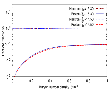
Figure 1: Particle fractions as a function of baryon number density $N$ for different values of $\tilde{g}_{\sigma}$.

In the FIG. 2, the effective mass of the neutron is plotted for different values of the scaled coupling constant $\tilde{g}_{\sigma}$. It may be observed that an increase of the parameter $\tilde{g}_{\sigma}$ leads the effective mass to decrease.

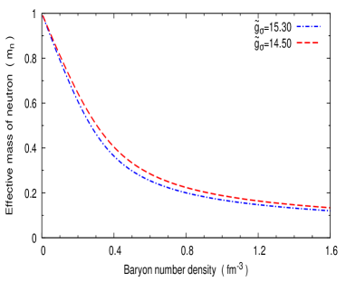
Figure 2: Effective mass of the neutron as a function of baryon number density $N$ for different values of coupling constant $\tilde{g}_{\sigma}$.

IV.2 Kinematical behavior of curved EOS

For different kinematical values of the metric function $\Phi$, pressure of the curved EOS (28) is plotted as a function of baryon number density $N$ in the FIG. 3. We note that for a given baryon number density, presence of the metric function $\Phi$ in the curved EOS leads to a reduction of the pressure, compared to its flat spacetime counterpart ($\Phi=0$). Similar behavior is seen also in the expression of the energy density (31).

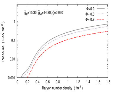
Figure 3: Plot of the pressure $P$ as a function of baryon number density $N$ for different kinematical values of $\Phi$.

Consequently, the presence of $e^{\Phi}$ factor in the expressions (28, 31) makes the pressure $P$ of the curved EOS comparatively stiffer for higher values of the energy density $\rho$. This behavior is shown in the FIG. 4 for different kinematical values of the metric function $\Phi$.

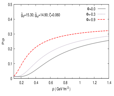
Figure 4: Ratio between the pressure and the energy density, $(P/\rho)$, is plotted as a function of $\rho$ for different kinematical values of the metric function $\Phi$.

We may emphasize that here we have chosen a set of fixed kinematical values of $\Phi$ while plotting the figures given in FIG. 3 and FIG. 4. However as follows from the TOV eqs. (2), the metric function $\Phi$ varies dynamically along the radial direction inside the stars.

IV.3 Numerical method for solving TOV eqs.

We note from the eq. (38) that number densities of the fermions, after solving for $\bar{\sigma}$, can be viewed as functions of neutron number density $n$ as $n_{I}=n_{I}(n)$. Therefore, the pressure (28) and the energy density (31) can be viewed as explicit functions of $n$ and $\Phi$, given as $P(n,\Phi)$ and $\rho(n,\Phi)$ respectively. Consequently, we can treat the TOV eqs. (2) as a set of first-order differential equations for the triplet $\{\mathcal{M},\Phi,n\}$ where the neutron number density $n$ satisfies

$$\frac{dn}{dr}=-\frac{(\rho+P+({\partial P}/{\partial\Phi}))}{({\partial P}/{\partial n})}\frac{d\Phi}{dr}~{}.$$ (39)

On the other hand, for the flat EOS, the pressure and the energy density are independent of $\Phi$ . Consequently, $\Phi$ can be eliminated from the set of TOV eqs. (2) which then can be viewed as a set of first-order differential equations for the doublet $\{\mathcal{M},n\}$.

For the curved EOS, nevertheless, the triplet $\{\mathcal{M},\Phi,n\}$ is subject to the boundary conditions $e^{2\Phi(R)}=(1-2GM/R)$, $M=\mathcal{M}(R)$ and $n(R)=0$ i.e. interior metric of a star of mass $M$ and radius $R$ must match with the Schwarzschild metric at the surface. In order to evolve the eq. (39) numerically, apart from $\rho$ and $P$, we also need to compute the terms $({\partial P}/{\partial\Phi})$ and $({\partial P}/{\partial n})$. In particular, the term $({\partial P}/{\partial n})$ can be expressed as

$$\frac{\partial P}{\partial n}=\sum_{I=n,p,e}\frac{\partial P_{I}}{\partial n_{I}}\frac{dn_{I}}{dn}+\frac{\partial P}{\partial\bar{\omega}}\frac{d\bar{\omega}}{dn}+\frac{\partial P}{\partial\bar{\sigma}}\frac{d\bar{\sigma}}{dn}~{},$$ (40)

where partial derivatives of $P$ w.r.t. $n_{I}$, $\bar{\omega}$ are

$$\frac{\partial P_{I}}{\partial n_{I}}=\frac{e^{\Phi}m_{I}^{*}(b_{I}n_{I})^{2/3}}{3\sqrt{(b_{I}n_{I})^{2/3}+1}}~{}~{},~{}\frac{\partial P}{\partial\bar{\omega}}=e^{\Phi}\Big{[}\bar{\omega}+\frac{\zeta}{6}\bar{g}_{\omega}^{4}\bar{\omega}^{3}\Big{]}~{},$$ (41)

respectively and partial derivative of $P$ w.r.t. $\bar{\sigma}$ is

$$\frac{\partial P}{\partial\bar{\sigma}}=-e^{\Phi}\bar{\sigma}+3\bar{g}_{\sigma}\sum_{I=n,p}\frac{n_{I}}{m_{I}^{*}}\left(\frac{\partial P_{I}}{\partial n_{I}}-\frac{4P_{I}}{3n_{I}}\right)~{}.$$ (42)

Total derivative of $\bar{\omega}$ (15) w.r.t. $n$ can be expressed as

$$\frac{d\bar{\omega}}{dn}=\frac{\zeta\bar{g}_{\omega}(2\zeta+w_{2}^{2})}{w_{1}w_{2}}\sum_{I=n,p}\frac{dn_{I}}{dn}~{}.$$ (43)

On the other hand, total derivatives of the number densities $n_{I}$ can be expressed as

$$\frac{dn_{I}}{dn}=\frac{\partial n_{I}}{\partial n}+\frac{\partial n_{I}}{\partial\bar{\sigma}}\frac{d\bar{\sigma}}{dn}~{},$$ (44)

where partial derivatives w.r.t. $n$ are

$$\frac{\partial n_{p}}{\partial n}=\frac{\partial n_{e}}{\partial n}=\frac{(b_{n}n)}{8}\frac{(b_{n}n)^{2/3}+2}{(\sqrt{(b_{n}n)^{2/3}+1})^{5}}~{},\frac{\partial n}{\partial n}=1~{},$$ (45)

and partial derivatives w.r.t. $\bar{\sigma}$ are given by

$$\frac{\partial n_{p}}{\partial\bar{\sigma}}=\frac{\partial n_{e}}{\partial\bar{\sigma}}=\frac{\bar{g}_{\sigma}m_{n}^{*2}}{8\pi^{2}}\frac{(b_{n}n)^{2}}{(\sqrt{(b_{n}n)^{2/3}+1})^{5}}~{},\frac{\partial n}{\partial\bar{\sigma}}=0~{}.$$ (46)

We have discussed earlier that one needs to solve for $\bar{\sigma}$ for a given neutron number density $n$. Once $\bar{\sigma}$ is found, the total derivative of $\bar{\sigma}$ can be expressed as

$$\frac{d\bar{\sigma}}{dn}=\bar{g}_{\sigma}\Big{[}\sum_{n,p}\frac{\partial n_{I}^{S}}{\partial n_{I}}\frac{\partial n_{I}}{\partial n}\Big{]}\Big{[}1-\bar{g}_{\sigma}\sum_{n,p}\Big{(}\frac{\partial n_{I}^{S}}{\partial\bar{\sigma}}+\frac{\partial n_{I}^{S}}{\partial n_{I}}\frac{\partial n_{I}}{\partial\bar{\sigma}}\Big{)}\Big{]}^{-1},$$ (47)

where partial derivatives of $n_{I}^{S}$ with w.r.t. $n$ and $\bar{\sigma}$ can be expressed as

$$\frac{\partial n_{I}^{S}}{\partial n_{I}}=\frac{1}{\sqrt{(b_{I}n_{I})^{2/3}+1}}~{},$$ (48)

and

$$\frac{\partial n_{I}^{S}}{\partial\bar{\sigma}}=-\frac{\bar{g}_{\sigma}m_{I}^{*2}}{\pi^{2}}\Big{[}(b_{I}n_{I}^{S})-\frac{(b_{I}n_{I})}{\sqrt{(b_{I}n_{I})^{2/3}+1}}\Big{]}~{}.$$ (49)

The eqs. (45, 46, 48, 49) completely determine the value of $d\bar{\sigma}/dn$ for a given value $n$ and $\bar{\sigma}$.

In summary, the TOV eqs. (2) here can be viewed as a well-defined boundary value problem. In order to satisfy the boundary condition numerically, we begin with a given central neutron number density, say $n_{c}$ and a trial value of $\Phi$ at the center. Subsequently, we evolve the TOV eqs. towards the surface by computing the meson field values $\bar{\sigma}$ and $\bar{\omega}$ at each step. This leads to an evolved value of $\Phi$ at the surface which is then compared with an independently calculated value of $\Phi$ at the surface by using the boundary condition, say, $\Phi_{s}=\tfrac{1}{2}\ln(1-2GM/R)$. In the next step, $\Phi$ at the center is numerically computed starting from the value $\Phi_{s}$ by evolving backward from $n=0$ at the surface to $n=n_{c}$ at the center by using the eq.

$$\frac{d\Phi}{dn}=-\frac{({\partial P}/{\partial n})}{(\rho+P+({\partial P}/{\partial\Phi}))}~{},$$ (50)

which follows from the eq. (39). These steps are iterated in order to achieve the convergence between the evolved and the computed values of the metric function $\Phi$ at the center within the desired numerical precision. The said iteration method converges rapidly except for the situations where the mass $M$ of the neutron star changes without appreciable change of the radius $R$. For these situations, one needs to employ an appropriate root finding method.

IV.4 Mass-radius relations

In the FIG. 5, we compare the mass-radius relations arising from both the curved EOS and the flat EOS for the $\sigma-\omega$ model and an ensemble of ideal non-interacting degenerate neutrons. It can be seen that irrespective of how the nuclear matters are described, the usage of the curved EOS, rather than the flat EOS, leads to a significantly higher mass limit.

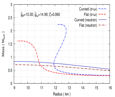
Figure 5: Comparison of mass-radius relations of neutron stars whose nuclear matters are described by the $\sigma-\omega$ model and an ensemble of non-interacting degenerate neutrons.

In the FIG. 6, we plot the dependency of neutron star mass $M$ on the central baryon number density for both the curved EOS and the flat EOS.

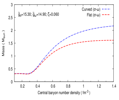
Figure 6: Plot of the neutron star mass $M$ as a function of the central baryon number density.

We have mentioned earlier that the equation of state corresponding to the $\sigma-\omega$ model, contains three independent parameters, namely $\tilde{g}_{\sigma}$, $\tilde{g}_{\omega}$, and $\zeta$. The parameter $\tilde{g}_{\sigma}$ changes the nature of the turning point of the mass-radius curve. An increase in the value of $\tilde{g}_{\sigma}$ changes the position of the turning point towards a smaller radius. Moreover, as the value of $\tilde{g}_{\sigma}$ increases, the radius of the neutron star with a given mass decreases and the maximum mass of the neutron star increases. The dependency of mass-radius relations on the parameter $\tilde{g}_{\sigma}$ is shown in the FIG. 7.

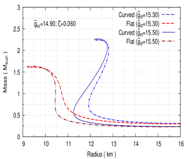
Figure 7: Plot of the mass-radius relations for different values of the parameter $\tilde{g}_{\sigma}$.

The parameter $\tilde{g}_{\omega}$ also changes the nature of the turning point of mass-radius curve. An increase in the value of $\tilde{g}_{\omega}$ changes position of the turning point towards a larger radius and after a certain value of $\tilde{g}_{\omega}$, the turning point disappears altogether. As the value of $\tilde{g}_{\omega}$ increases, radius of the neutron star with a given mass increases. Moreover, as the value of $\tilde{g}_{\omega}$ increases, the maximum mass of neutron star decreases. This behavior is shown in the FIG. 8.

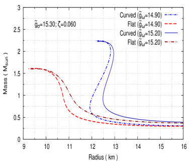
Figure 8: Plot of the mass-radius relations for different values of the parameter $\tilde{g}_{\omega}$.

On the other hand, the parameter $\zeta$ changes the maximum mass and the corresponding radius without much alteration in the nature of mass-radius curve. An increase in the value of $\zeta$ causes the maximum mass limit of the neutron stars to decrease. Moreover, as the value of $\zeta$ increases, the radius of neutron star for a given mass decreases. This aspect is shown in the FIG. 9.

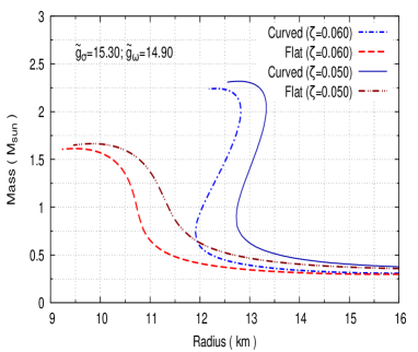
Figure 9: Plot of the mass-radius relations for different values of the parameter $\zeta$.

Clearly, in all these mass-radius relations, a significant enhancement of the maximum mass limits can be seen when one uses the curved EOS rather than the flat EOS. A quantitative comparison of the computed mass limits and the corresponding radii of the neutron stars are given in the TABLE LABEL:table:ParameterTable. As an example, it can be seen that the flat EOS with the parameter values $\tilde{g}_{\sigma}=15.30$, $\tilde{g}_{\omega}=14.90$, and $\zeta=0.06$ leads the maximum mass limit to be around $1.61M_{\odot}$ with radius of $9.50$ km. On the other hand, the curved EOS with the same set of parameters leads the maximum mass limit to be around $2.24M_{\odot}$ with a radius of around $12.33$ km. Thus incorporation of the effect of gravitational time dilation enhances the maximum mass limit here by almost $39.1\%$. The corresponding increase in radius of the star is around $29.8\%$. These enhancements of mass limits are controlled quantitatively by the ratio $(GM/R)$ of the star and follow from the equation of state (28, 31) as $\rho_{curved}(r+\Delta r)>\rho_{flat}(r+\Delta r)$ even if $\rho_{curved}(r)=\rho_{flat}(r)$ and $(\tfrac{\partial\rho_{curved}}{\partial n}\tfrac{dn}{dr})_{|r}=(\tfrac{\partial\rho_{flat}}{\partial n}\tfrac{dn}{dr})_{|r}$ given $(d\Phi/dr)>0$ for $\Delta r>0$ Hossain and Mandal (2021).

Table 1: The maximum mass limits and the corresponding radii of neutron stars for both curved EOS and flat EOS of the $\sigma-\omega$ model for different parameter sets.

$\tilde{g}_{\sigma}$	$\tilde{g}_{\omega}$	$\zeta$	$M~{}(M_{\odot})$		$R~{}(km)$
			flat	curved	flat	curved
15.30	14.90	0.060	1.61	2.24	9.50	12.33
15.30	15.20	0.060	1.60	2.23	9.59	12.40
15.30	14.90	0.050	1.66	2.32	9.84	12.79
15.50	14.90	0.060	1.63	2.27	9.45	12.30
14.50	14.70	0.060	1.56	2.16	9.63	12.35
15.90	14.90	0.020	2.00	2.85	11.24	14.87

We would like to note here that for another chosen set of parameters, the flat EOS corresponding to the $\sigma-\omega$ model leads to a maximum mass limit of around $2M_{\odot}$. On the other hand, the corresponding curved EOS with the same set of parameters leads the maximum mass limit of neutron stars to be around $2.85M_{\odot}$. These two mass-radius curves are plotted in the FIG. 10.

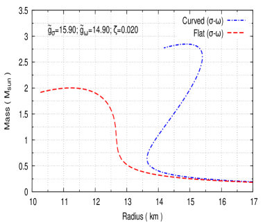
Figure 10: Comparison of mass-radius relations of neutron stars whose nuclear matters are described by the $\sigma-\omega$ model with a chosen set of parameters such that both flat EOS and curved EOS leads the mass limits to be $2M_{\odot}$ or higher.

V Universal effect of gravitational time dilation

We have seen that the usage of flat EOS fails to capture the effect of gravitational time dilation. This aspect can be understood in a rather simple way. While solving the TOV eqs. (2), one evolves from the center to the surface of the star. In this process, the metric function $\Phi$ changes considerably. Consequently, the clock speed in a locally flat spacetime near the center of the star differs from the clock speed of a locally flat spacetime near the surface of the star, given these two frames have different lapse functions, $e^{\Phi(r=0)}$ and $e^{\Phi(r=R)}$ respectively. An equation of state which is computed in a globally flat spacetime fails to capture this varying nature of the lapse function or the resultant varying clock speed. On the other hand, the curved EOS, as studied here, incorporates the gravitational time dilation through the presence of metric function $\Phi$ in the expressions of pressure and energy density (28, 31).

Nevertheless, it is shown in Hossain and Mandal (2021) that it is possible to obtain the equation of state for a spherically symmetric curved spacetime starting from its flat spacetime counterpart without going through a first-principle derivation. In particular, to obtain the partition function in a spherically symmetric spacetime, one needs to use the following transformations Hossain and Mandal (2021)

$$\beta\rightarrow\beta e^{\Phi}~{},~{}~{}\mu_{I}\rightarrow\mu_{I}e^{-\Phi}~{}.$$ (51)

The transformation rules (51)can be understood as follows. By re-defining the time coordinate $t\to\tilde{t}=e^{\Phi}t$, one can transform the metric (9) within the box to be the standard Minkowski metric. Consequently, at thermal equilibrium, the anti-periodic boundary condition for the spinor fields, as employed in the eq. (24), then leads to the transformation rules (51). The universality of the transformations (51) can be checked from the general expression of the partition function in the Minkowski spacetime which can always be written as

$$\ln\mathcal{Z}_{\text{flat}}[\beta,\{\mu_{I}\},\{\lambda_{i}\}]=\beta^{-3}Vf(\{\beta\mu_{I}\},\{\beta^{d_{i}}\lambda_{i}\})~{},$$ (52)

where $\{\lambda_{i}\}$ is a set of parameters of an interacting matter field theory, having canonical mass dimensions $\{d_{i}\}$. For example, in the $\sigma-\omega$ model that we have studied here, the canonical mass dimensions of the coupling constants $\{g_{\sigma},g_{\omega},\zeta\}$ are zero whereas the canonical mass dimensions of $\omega$ and $\sigma$ fields are one. The general form (52) follows from the fact that $\ln\mathcal{Z}$ is a dimensionless, extensive quantity in statistical physics. Therefore, by following the transformation rules (51), we can obtain the partition function in a spherically symmetric curved spacetime as

$$\ln\mathcal{Z}[\beta,\{\mu_{I}\},\{\lambda_{i}\}]=e^{-3\Phi}\ln\mathcal{Z}_{\text{flat}}[\beta,\{\mu_{I}\},\{e^{d_{i}\Phi}\lambda_{i}\}]~{}.$$ (53)

The eq. (53) can be used to obtain the partition function of the $\sigma-\omega$ model (20) starting from its flat spacetime counterpart. It also shows that the different choices of frames for intermediate computation eventually lead to the same equation of state for the curved spacetime.

VI Discussions

In summary, by employing a first-principle approach, we have derived the equation of state for a degenerate nuclear matter which is described by a simplified $\sigma-\omega$ model. Importantly, in this derivation the nuclear matter is assumed to reside within the spherically symmetric interior curved spacetime of the neutron star, rather than in the Minkowski spacetime as routinely used in the literature. The equation of state which is computed in the curved spacetime, includes the effect of gravitational time dilation. Furthermore, we have shown that the incorporation of gravitational time dilation significantly increases the maximum mass limits of neutron stars. As an example, the $\sigma-\omega$ model with a chosen set of parameters, leads the maximum mass limit to be around $1.61M_{\odot}$ when one uses the equation of state computed in the Minkowski spacetime. In contrast, with the same set of parameters, the equation of state computed in the curved spacetime, leads the maximum mass limit to be around $2.24M_{\odot}$, a significant increase of $\sim 39.1\%$.

Recent observations of several neutron stars having masses more than $2M_{\odot}$, have pushed many existing models of nuclear matters within the neutron stars, to be ruled out Linares et al. (2018); Cromartie et al. (2020). However, as we have shown here that a proper incorporation of gravitational time dilation into the corresponding equation of states would enhance the maximum mass limits of such models.

Finally, we would like to emphasize here that the existence of the gravitational time dilation is a universal feature of the curved spacetime. Therefore, the effect of gravitational time dilation as studied here, should be included any model of nuclear matter within the neutron stars.

Acknowledgments: SM would like to thank IISER Kolkata for supporting this work through a doctoral fellowship.

References

- Hossain and Mandal (2021) G. M. Hossain and S. Mandal, Journal of Cosmology and Astroparticle Physics 2021, 026 (2021).
- Shapiro and Teukolsky (2008) S. Shapiro and S. Teukolsky, Black Holes, White Dwarfs, and Neutron Stars: The Physics of Compact Objects (Wiley, 2008).
- Nättilä et al. (2017) J. Nättilä, M. Miller, A. Steiner, J. Kajava, V. Suleimanov, and J. Poutanen, Astronomy & Astrophysics 608, A31 (2017).
- Özel et al. (2016) F. Özel, D. Psaltis, T. Güver, G. Baym, C. Heinke, and S. Guillot, The Astrophysical Journal 820, 28 (2016).
- Shen (2002) H. Shen, Physical Review C 65, 035802 (2002).
- Lattimer and Prakash (2016) J. M. Lattimer and M. Prakash, Physics Reports 621, 127 (2016).
- Douchin and Haensel (2001) F. Douchin and P. Haensel, Astronomy & Astrophysics 380, 151 (2001).
- Tolos et al. (2016) L. Tolos, M. Centelles, and A. Ramos, The Astrophysical Journal 834, 3 (2016).
- Maieron et al. (2004) C. Maieron, M. Baldo, G. Burgio, and H.-J. Schulze, Physical Review D 70, 043010 (2004).
- Klähn et al. (2007) T. Klähn, D. Blaschke, F. Sandin, C. Fuchs, A. Faessler, H. Grigorian, G. Röpke, and J. Trümper, Physics Letters B 654, 170 (2007).
- Baldo et al. (2007) M. Baldo, G. Burgio, P. Castorina, S. Plumari, and D. Zappala, Physical Review C 75, 035804 (2007).
- Whittenbury et al. (2014) D. Whittenbury, J. Carroll, A. Thomas, K. Tsushima, and J. Stone, Physical Review C 89, 065801 (2014).
- Katayama et al. (2012) T. Katayama, T. Miyatsu, and K. Saito, The Astrophysical Journal Supplement Series 203, 22 (2012).
- Miyatsu et al. (2013) T. Miyatsu, S. Yamamuro, and K. Nakazato, The Astrophysical Journal 777, 4 (2013).
- Chatterjee and Vidana (2016) D. Chatterjee and I. Vidana, The European Physical Journal A 52, 1 (2016).
- Schaffner-Bielich (2008) J. Schaffner-Bielich, Nuclear Physics A 804, 309 (2008).
- Balberg et al. (1999) S. Balberg, I. Lichtenstadt, and G. B. Cook, The Astrophysical Journal Supplement Series 121, 515 (1999).
- Dhapo et al. (2010) H. Dhapo, B.-J. Schaefer, and J. Wambach, Physical Review C 81, 035803 (2010).
- Bednarek and Manka (2001) I. Bednarek and R. Manka, International Journal of Modern Physics D 10, 607 (2001).
- Hornick et al. (2018) N. Hornick, L. Tolos, A. Zacchi, J.-E. Christian, and J. Schaffner-Bielich, Physical Review C 98, 065804 (2018).
- Serot (1992) B. D. Serot, Reports on Progress in Physics 55, 1855 (1992).
- Serot and Walecka (1997) B. D. Serot and J. D. Walecka, International Journal of Modern Physics E 6, 515 (1997).
- Dvornikov (2019) M. Dvornikov, Physical Review D 99, 116021 (2019).
- Andersen and Strickland (2005) J. O. Andersen and M. Strickland, Annals of Physics 317, 281 (2005).
- Sterman and Tejeda-Yeomans (2003) G. Sterman and M. E. Tejeda-Yeomans, Physics Letters B 552, 48 (2003).
- Ring (1996) P. Ring, Progress in Particle and Nuclear Physics 37, 193 (1996).
- Mueller and Serot (1996) H. Mueller and B. D. Serot, Nuclear Physics A 606, 508 (1996).
- Matsubara (1955) T. Matsubara, Progress of theoretical physics 14, 351 (1955).
- Kapusta and Gale (2006) J. I. Kapusta and C. Gale, Finite-temperature field theory: Principles and applications (Cambridge University Press, 2006).
- Das (1997) A. K. Das, Finite Temperature Field Theory (World Scientific, New York, 1997).
- Toms (1987) D. J. Toms, Physical Review D 35, 3796 (1987).
- Visser (2017) M. Visser, arXiv:1702.05572 (2017).
- Lim et al. (2018) Y. Lim, C.-H. Lee, and Y. Oh, Physical Review D 97, 023010 (2018).
- Linares et al. (2018) M. Linares, T. Shahbaz, and J. Casares, The Astrophysical Journal 859, 54 (2018).
- Cromartie et al. (2020) H. T. Cromartie, E. Fonseca, S. M. Ransom, P. B. Demorest, Z. Arzoumanian, H. Blumer, P. R. Brook, M. E. DeCesar, T. Dolch, J. A. Ellis, et al., Nature Astronomy 4, 72 (2020).