Low-rank tensor recovery
for Jacobian-based Volterra identification
of parallel Wiener-Hammerstein systems

Abstract

We consider the problem of identifying a parallel Wiener-Hammerstein structure from Volterra kernels. Methods based on Volterra kernels typically resort to coupled tensor decompositions of the kernels. However, in the case of parallel Wiener-Hammerstein systems, such methods require nontrivial constraints on the factors of the decompositions. In this paper, we propose an entirely different approach: by using special sampling (operating) points for the Jacobian of the nonlinear map from past inputs to the output, we can show that the Jacobian matrix becomes a linear projection of a tensor whose rank is equal to the number of branches. This representation allows us to solve the identification problem as a tensor recovery problem.

1 Introduction

Nonlinear identification methods that go beyond the well-established linear system identification tools (Pintelon and Schoukens, 2012; Ljung, 1999; Katayama, 2005), are steadily gaining research attention in recent years. Advances in nonlinear modeling tools, combined with the ever increasing computing power allows for the exploration of nonlinear models that account for nonlinear effects that occur when pushing systems outside of their linear operating regions. There is a host of procedures that range from simple extensions of linear models, over nonlinear state space modeling (possibly using particle filtering), to variations on neural network architectures, each of which typically require tailored nonconvex optimization methods. While such models may provide satisfactory prediction results, their internal workings are often hard to assess, which makes them difficult to use and interpret.

The current paper considers a combination of two promising nonlinear models (block-oriented models and Volterra series), and aims at combining their advantages while avoiding the drawbacks. Block-oriented systems are composed as interconnections of linear time-invariant system blocks and static nonlinearities such as the well-known Wiener, Hammerstein, Wiener-Hammerstein and Hammerstein-Wiener systems (Giri and Bai, 2010). A block-oriented system description strikes a balance between flexibility and model interpretability: the model accounts for (strong) nonlinearities in its description, but stays close to the familiar linear world and allows for a transparent understanding of its workings. Nevertheless, block-oriented system identification methods rely on heuristics and nonconvex optimization routines (Schoukens and Tiels, 2017) to find the parameters, which may cause difficulties. Volterra series models, on the other hand, can be viewed as nonlinear extensions of the well-known convolution operation of the input signal with the (finite) impulse response: in the Volterra description, the output is defined as a polynomial function of (delayed) inputs (as opposed to the output being a linear function of delayed inputs in the case of linear systems). A major advantage is that the Volterra model is linear in the parameters and its identification can be posed as a least-squares problem (Birpoutsoukis et al., 2017). Unfortunately, due to the polynomial structure, the number of coefficients grows very quickly as the polynomial degree increases. In addition, the model does not allow for an intuitive understanding of its internal operation.

Figure 1: Parallel Wiener-Hammerstein system.

In this article, we are interested in identification of discrete-time parallel Wiener-Hammerstein systems, see Fig. 1. Each branch of such a system has a Wiener-Hammerstein structure, i.e., a static nonlinearity sandwiched in between two linear time-invariant (LTI) blocks. Parallel Wiener-Hammerstein models have improved approximation properties as opposed to single branch Wiener-Hammerstein models (Palm, 1979). However, identification of a parallel Wiener-Hammerstein structure is particularly challenging, see Schoukens and Tiels (2017). For example, the frequency-domain methods (Schoukens and Tiels, 2017) suffer from the pole/zero mixing of the Wiener and Hammerstein filters, and thus require a computationally heavy pole/zero splitting procedure.

The method that we present in this article starts from estimating Volterra kernels, which can be readily viewed as higher-order symmetric tensors containing the polynomial coefficients. Existing methods that aim at finding block-oriented models from the Volterra kernels resort to coupled tensor decompositions of Volterra kernels (Kibangou and Favier, 2007) and require nontrivial constraints on the factors of the tensor decomposition for parallel Wiener-Hammerstein case (Dreesen et al., 2017; Westwick et al., 2017; Dreesen and Ishteva, 2021). In this paper, we propose an entirely different approach: by choosing special sampling points, we can show that the Jacobian matrix becomes a linear projection of a certain low-rank tensor whose rank is equal to the number of parallel branches in the model. This representation allows us to solve the identification problem as a tensor recovery problem, which may be approached by an alternating least squares (ALS) solution strategy.

2 Preliminaries

2.1 Tensor and vector notation

In this paper we mainly follow Comon (2014) in what concerns tensor notation (see also Kolda and Bader (2009)). We use lowercase ($a$) or uppercase ($A$) plain font for scalars, boldface lowercase ($\boldsymbol{a}$) for vectors, uppercase boldface ($\boldsymbol{A}$) for matrices, calligraphic font ($\boldsymbol{\mathcal{A}}$) for $N$-D arrays (tensors) and script ($\mathscr{P}$) for operators. Vectors are, by convention, one-column matrices. The elements of vectors/matrices/tensors are accessed as $a_{i}$, ${A}_{i,j}$ and $\mathcal{A}_{i_{1},\ldots,i_{N}}$ respectively. We use $\mathop{\operator@font vec}\{\cdot\}$ for the standard column-major vectorization of a tensor or a matrix. Operator $\mathop{\bullet}_{p}$ denotes the contraction on the $p$th index of a tensor, i.e.,

$$[\boldsymbol{\mathcal{A}}\mathop{\bullet}_{1}\boldsymbol{u}]_{jk}=\sum_{i}\mathcal{A}_{ijk}u_{i}.$$

For a matrix ${\boldsymbol{A}}$, ${\boldsymbol{A}}^{{\sf T}}$ and ${\boldsymbol{A}}^{\dagger}$ denotes its transpose and Moore-Penrose pseudoinverse respectively. The notation ${\boldsymbol{I}}_{M}$ is used for the $M\times M$ identity matrix and $\boldsymbol{0}_{L\times K}$ for the $L\times K$ matrix of zeroes. We use the symbol $\mathop{\boxtimes}$ for the Kronecker product of matrices (in order to distinguish it from the tensor product $\otimes$), and $\odot$ for the (column-wise) Khatri-Rao product of matrices: i.e, the Khatri-Rao product of

$$\boldsymbol{A}=\begin{bmatrix}\boldsymbol{a}_{1}&\cdots&\boldsymbol{a}_{r}\end{bmatrix}\quad\text{and}\quad\boldsymbol{B}=\begin{bmatrix}\boldsymbol{b}_{1}&\cdots&\boldsymbol{b}_{r}\end{bmatrix}$$

is defined as

$${\boldsymbol{A}}\odot{\boldsymbol{B}}=\begin{bmatrix}\boldsymbol{a}_{1}\mathop{\boxtimes}\boldsymbol{b}_{1}&\cdots&\boldsymbol{a}_{r}\mathop{\boxtimes}\boldsymbol{b}_{r}\end{bmatrix}.$$

We use the notaion $\mathop{\operator@font Diag}\{\boldsymbol{v}\}$ for the diagonal matrix built from the vector $\boldsymbol{v}$.

A polyadic decomposition (PD) is a decomposition of a tensor into a sum of rank-one terms, i.e., for $\boldsymbol{\mathcal{Y}}\in\mathbb{R}^{I\times J\times K}$,

$$\boldsymbol{\mathcal{Y}}=\sum\limits_{\ell=1}^{r}\boldsymbol{a}_{\ell}\otimes\boldsymbol{b}_{\ell}\otimes\boldsymbol{c}_{\ell}$$ (1)

is a polyadic decomposition. It is called canonical polyadic (CPD) if the number $r$ in (1) is minimal among all possible PDs of $\boldsymbol{\mathcal{Y}}$; in that case $r$ is called the tensor rank of $\boldsymbol{\mathcal{Y}}$.

By grouping vectors into matrices

$$\boldsymbol{A}=\begin{bmatrix}\boldsymbol{a}_{1}&\cdots&\boldsymbol{a}_{r}\end{bmatrix},\quad\boldsymbol{B}=\begin{bmatrix}\boldsymbol{b}_{1}&\cdots&\boldsymbol{b}_{r}\end{bmatrix},\quad\boldsymbol{C}=\begin{bmatrix}\boldsymbol{c}_{1}&\cdots&\boldsymbol{c}_{r}\end{bmatrix}$$

we can use a more compact notation

$$\boldsymbol{\mathcal{Y}}=[\![{\boldsymbol{A}},{\boldsymbol{B}},{\boldsymbol{C}}]\!],\quad\mathcal{Y}_{ijk}=\sum\limits_{\ell=1}^{r}A_{i\ell}B_{j\ell}C_{k\ell};$$

for a PD (or a CPD).

Finally, for a (possibly finite) sequence

$$(\ldots,x(1),\ldots,x(T),\ldots)$$

its convolution with a vector $\boldsymbol{a}\in\mathbb{R}^{K}$ is defined as

$$(\boldsymbol{a}\ast x)(t)=\sum\limits_{i=1}^{K}x(t-i+1)a_{i}.$$

2.2 Volterra kernels

The Volterra series (Schetzen, 1980) is a classical model for nonlinear systems, and is similar to the Taylor expansion for multivariate maps. In the discrete-time case, Volterra series can be interpreted as a power series expansion of the output of a system as a function of past inputs: $y(t)=f^{(0)}+$

$$\sum\limits^{\infty}_{s=1}\left(\sum^{\infty}_{\tau_{1}=0}\cdots\sum^{\infty}_{\tau_{s}=0}H^{(s)}(\tau_{1},\ldots,\tau_{s})u(t-\tau_{1})\cdots u(t-\tau_{s})\right),$$

where $H^{(s)}(\cdot)$ is the $s$-th order Volterra kernel. In the special case when the output depends only on a finite number $L$ of past inputs, i.e., is defined by $f:\mathbb{R}^{L}\to\mathbb{R}$

$$y(t)=f(u({t}),u({t-1}),\ldots,u({t-L+1})),$$ (2)

we can consider truncated the Volterra kernels $\boldsymbol{\mathcal{H}}^{(s)}$ (which are $L\times\cdots\times L$ tensors). By denoting for convenience the vector of past inputs as

$$\boldsymbol{u}=\begin{bmatrix}u({t})&u({t-1})&\ldots&u({t-L+1})\end{bmatrix}^{{\sf T}}$$ (3)

we can write the function expansion as

$$y({t})=f(\boldsymbol{u})=f^{(0)}+f^{(1)}(\boldsymbol{u})+\cdots+f^{(d)}(\boldsymbol{u})+\cdots,$$ (4)

where the degree-$s$ term is given by

$$f^{(s)}(\boldsymbol{u})=\sum_{i_{1},\ldots,i_{s}=1}^{L,\ldots,L}\mathcal{H}^{(s)}_{i_{1},\ldots,i_{s}}u({t}-i_{1}+1)\cdots u({t}-i_{s}+1),$$

with

$$\mathcal{H}^{(s)}_{i_{1},\ldots,i_{s}}=H^{(s)}(i_{1}-1,\ldots,i_{s}-1).$$

Order-$s$ terms can be compactly expressed using the multiple contraction

$$f^{(s)}(\boldsymbol{u})=\boldsymbol{\mathcal{H}}^{(s)}\mathop{\bullet}_{1}\boldsymbol{u}\mathop{\bullet}_{2}\boldsymbol{u}\cdots\mathop{\bullet}_{s}\boldsymbol{u}.$$

2.3 Parallel Wiener-Hammerstein model

In this paper, we consider the case when the LTI blocks in Fig. 1 are given by finite impulse response (FIR) filters of lags $L_{1}$ and $L_{2}$ respectively. Formally, the output $y(t)$ at a time instant $t$ of a parallel Wiener-Hammerstein system is given by a composition of convolutions and univariate nonlinear transformations:

$$y=\sum\limits_{\ell=1}^{r}\boldsymbol{b}_{\ell}\ast{z}_{\ell},\quad z_{\ell}=g_{\ell}(x_{\ell}),\quad x_{\ell}=\boldsymbol{a}_{\ell}\ast u,$$

where $\boldsymbol{a}_{\ell}\in\mathbb{R}^{L_{1}}$, $\boldsymbol{b}_{\ell}\in\mathbb{R}^{L_{2}}$, $g_{\ell}:\mathbb{R}\to\mathbb{R}$. In this case, it is easy to see that the output $y(t)$ of the system depends only on $L=L_{1}+L_{2}-1$ past inputs, i.e., $\boldsymbol{u}$ in (3).

In this paper, we also add another simplifying assumption that each $g_{\ell}(t)$ is a polynomial of degree $d$. Therefore, the function $f$ in (2) is a degree-$d$ polynomial and thus the system is completely characterized by the first $d$ truncated $L\times\cdots\times L$ Volterra kernels (i.e., by the collection of the homogeneous terms $f^{(s)}$ up to degree $d$, see (4)).

3 First-order information and projection

3.1 An overview of the proposed approach

Our main idea is to exploit the first-order information in spirit of the method in Dreesen et al. (2015). The original method of Dreesen et al. (2015) is designed for decoupling a static nonlinear function $f$ based on the evaluations of the first-order derivatives (Jacobians) of $f$ at a chosen set of operating points $\boldsymbol{u}^{(1)},\ldots,\boldsymbol{u}^{(N)}$, by stacking these evaluations in a 3rd order tensor and performing its CPD.

Note that in case of a polynomial map (2), the derivatives can be easily computed from the Volterra kernels thanks to the following identity for degree-$s$ parts:

$$\nabla f^{(s)}(\boldsymbol{u})=s\cdot\boldsymbol{\mathcal{H}}^{(s)}\mathop{\bullet}_{2}\boldsymbol{u}\cdots\mathop{\bullet}_{s}\boldsymbol{u}.$$ (5)

However, a direct application of the decoupling technique is not possible in our case due to the following issues:

• the method of Dreesen et al. (2015) does not take into account the dynamics;

• the method of Dreesen et al. (2015) is not applicable to single-output functions (the Jacobian tensor becomes a matrix).

Some remedies for these issues were proposed in the literature. For example, Usevich (2014) reformulated the problem as structured matrix completion, Hollander (2017) introduced constraints on the factors of the CPD, while Dreesen et al. (2018) considered tensors of higher-order derivatives. However, none of these approaches provide an out-of-the box solution for our identification problem.

In this paper, we propose an entirely different approach. We use only the first-order information of $f$; however, we split $f$ into homogeneous parts (4) in the spirit of Van Mulders et al. (2014). A particular choice of tailored operating points (see subsection 3.3) allows us to show that the vector of evaluations of the gradients of the homogeneous parts can be viewed as a linear projection (sampling) of a third-order tensor $\boldsymbol{\mathcal{T}}$ whose rank is equal to the number of branches and whose factors give the coefficients for the filters in the LTI blocks. This allows us to reformulate the identification problem as a low-rank tensor recovery problem.

The remainder of this paper is organized as follows. In the current section, we focus only on the case of a single branch. We begin by some preliminary observations, followed by describing the structure of the tailored operating points. For such points, we then describe the building blocks for the projection operator in subsection 3.4 and show in subsection 3.5 that the vector of gradient evaluations is a projection of a rank-one tensor. The overall algorithm for $r$ branches is presented in section 4, where an algorithm for tensor recovery is also dicussed. The numerical experiments are provided in section 5.

3.2 Single branch: preliminary observations

We consider the case of a single branch, with the filters

$$\boldsymbol{a}=\begin{bmatrix}a_{1},\ldots,a_{L_{1}}\end{bmatrix}^{{\sf T}},\quad\boldsymbol{b}=\begin{bmatrix}b_{1},\ldots,b_{L_{2}}\end{bmatrix}^{{\sf T}}$$

and the single (not necessarily homogeneous) nonlinearity $g(t)$. Then, the output of a single branch is given by (2) with the nonlinear map

$$f(\boldsymbol{u})=\boldsymbol{b}^{\top}\boldsymbol{g}(\boldsymbol{V}^{{\sf T}}\boldsymbol{u}),$$

where $\boldsymbol{g}(\cdot)$ is defined as

$$\boldsymbol{g}(x_{1},\ldots,x_{L_{1}})=\begin{bmatrix}g(x_{1})&\ldots&g(x_{L_{1}})\end{bmatrix}^{{\sf T}},$$

and $\boldsymbol{V}\in\mathbb{R}^{L\times L_{2}}$ is the following Toeplitz matrix:

$$\boldsymbol{V}=\begin{bmatrix}\boldsymbol{v}_{1}&\cdots&\boldsymbol{v}_{L_{2}}\end{bmatrix}=\begin{bmatrix}a_{1}&&\\ \vdots&\ddots&\\ a_{L_{1}}&&a_{1}\\ &\ddots&\vdots\\ &&a_{L_{1}}\\ \end{bmatrix}.$$ (6)

By the chain rule (as in Dreesen et al. (2015)), the gradient of $f$ has the form

$$\nabla f(\boldsymbol{u})=\boldsymbol{V}\begin{bmatrix}g^{\prime}(\boldsymbol{v}_{1}^{{\sf T}}\boldsymbol{u})&&\\ &\ddots&\\ &&g^{\prime}(\boldsymbol{v}_{L_{2}}^{{\sf T}}\boldsymbol{u})\end{bmatrix}\boldsymbol{b}.$$ (7)

Remark 1

Although the function $f$, the model of the dynamical system, and the Volterra kernels were initially defined for real inputs, the expressions in (5) and (7) are polynomial in $\boldsymbol{u}$, hence we can formally evaluate them at complex points $\boldsymbol{u}\in\mathbb{C}^{L}$. This is one of the important features of our approach that allows us to avoid some numerical issues.

3.3 Tailored operation points

Next, we restrict our attention to homogeneous parts of the nonlinearity $g(x)=cx^{s}$. Another key idea of our method is to use tailored operating points $\boldsymbol{u}\in\mathbb{C}^{L}$ in order to simplify the expression in (7). We are going to use Vandermonde-like operating points parameterized by $\mu\in\mathbb{C}$:

$$\boldsymbol{u}_{\mu}=\begin{bmatrix}{1}&\mu&\mu^{2}&\ldots&\mu^{L-1}\end{bmatrix}^{{\sf T}}.$$

In this case, it is not difficult to see that

$$g^{\prime}(\boldsymbol{v}_{k}^{{\sf T}}\boldsymbol{u}_{\mu}) =cs(\boldsymbol{v}_{k}^{{\sf T}}\boldsymbol{u}_{\mu})^{s-1}$$

$$=cs(\mu^{k-1}a(\mu))^{s-1}=cs\mu^{(k-1)(s-1)}(a(\mu))^{s-1},$$

where $a(\mu)=a_{1}+a_{2}\mu+\cdots+a_{L_{1}}\mu^{L_{1}-1}$. Plugging this expression in (7), we obtain that

$$\nabla f^{(s)}(\boldsymbol{u}_{\mu})=(cs(a(\mu))^{s-1})\boldsymbol{v}_{\mu}$$ (8)

where the vector $\boldsymbol{v}_{\mu}\in\mathbb{C}^{L}$ is defined as

$$\boldsymbol{v}_{\mu}=\boldsymbol{V}\begin{bmatrix}b_{1}\\ b_{2}\mu^{(s-1)}\\ \vdots\\ b_{L_{2}}\mu^{(L_{2}-1)(s-1)}\end{bmatrix}$$

$$=\begin{bmatrix}a_{1}b_{1}\\ a_{2}b_{1}+a_{1}b_{2}\mu^{(s-1)}\\ a_{3}b_{1}+a_{2}b_{2}\mu^{(s-1)}+a_{1}b_{3}\mu^{2(s-1)}\\ \vdots\\ a_{L_{1}}b_{L_{2}-1}\mu^{(L_{2}-2)(s-1)}+a_{L_{1}-1}b_{L_{2}}\mu^{(L_{2}-1)(s-1)}\\ a_{L_{1}}b_{L_{2}}\mu^{(L_{2}-1)(s-1)}\end{bmatrix},$$

where $\boldsymbol{V}$ is defined in (6).

3.4 Gradient as a projection of a rank-one term

We are going to show that $\boldsymbol{v}_{\mu}$ from the previous subsection can be conveniently written as a linear projection (sampling) of a rank-one matrix. First of all, we introduce the diagonal summation (“Hankelization”) operator $\mathscr{H}:\mathbb{C}^{L_{1}\times L_{2}}\to\mathbb{C}^{L}$, which takes the sums on the antidiagonals

$$\mathscr{H}(\boldsymbol{E})=\begin{bmatrix}E_{1,1}\\ E_{2,1}+E_{1,2}\\ E_{3,1}+E_{2,2}+E_{1,3}\\ \vdots\\ E_{L_{1},L_{2}-1}+E_{L_{1}-1,L_{2}}\\ E_{L_{1},L_{2}}\end{bmatrix}.$$

Next, it is easy to see that $\boldsymbol{v}_{\mu}$ can be obtained by applying the projection operator $\mathscr{P}_{\mu,s}:\mathbb{C}^{L_{1}\times L_{2}}\to\mathbb{C}^{L}$, which is a composition of the diagonal summation with the scaling of columns by powers of $\mu$:

$$\mathscr{P}_{\mu,s}(\boldsymbol{E})=\mathscr{H}(\boldsymbol{E}\mathop{\operator@font Diag}\{\begin{bmatrix}1&\mu^{(s-1)}&\cdots&\mu^{(L_{2}-1)(s-1)}\end{bmatrix}\}),$$

i.e., $\boldsymbol{v}_{\mu}=\mathscr{P}_{\mu,s}(\boldsymbol{a}\boldsymbol{b}^{{\sf T}})$. After that, we get that the gradient in (8) can be expressed as follows

$$\nabla f^{(s)}(\boldsymbol{u}_{\mu})=\mathscr{P}_{\mu,s}((cs(a(\mu))^{s-1})\boldsymbol{a}\boldsymbol{b}^{{\sf T}}).$$

Finally, in the next subsections we are going to evaluate the gradients at different operating points and collect information from several kernels.

3.5 Combining several kernels and points

Now consider a set of $N$ points in the complex plane

$$\{\mu_{1},\ldots,\mu_{N}\}\subset\mathbb{C}$$

at which we are evaluating the gradients of the homogeneous parts, and collecting them into one single vector:

$$\boldsymbol{y}=\begin{bmatrix}\nabla f^{(1)}(\boldsymbol{u}_{1})\\ \nabla f^{(2)}(\boldsymbol{u}_{\mu_{1}})\\ \vdots\\ \nabla f^{(2)}(\boldsymbol{u}_{\mu_{N}})\\ \vdots\\ \nabla f^{(d)}(\boldsymbol{u}_{\mu_{1}})\\ \vdots\\ \nabla f^{(d)}(\boldsymbol{u}_{\mu_{N}})\\ \end{bmatrix}\in\mathbb{C}^{((d-1)N+1)L}.$$ (9)

Unlike the previous section, we now consider a general polynomial nonlinearity:

$$g(t)=c_{1}t+c_{2}t^{2}+\cdots+c_{d}t^{d}.$$

By using the results of the previous subsection, we can show that $y$ is a projection of a rank-1 tensor:

$$\boldsymbol{y}=\mathscr{P}(\boldsymbol{\mathcal{T}}),$$

where the rank-one tensor is

$$\boldsymbol{\mathcal{T}}=\boldsymbol{a}\otimes\boldsymbol{b}\otimes\boldsymbol{h},$$

vectors $\boldsymbol{a}$, $\boldsymbol{b}$ are as before, and $\boldsymbol{h}^{{\sf T}}=$

$$\begin{bmatrix}c_{1}&2c_{2}a(\mu_{1})&\!\!\cdot\cdot&2c_{2}a(\mu_{N})&\!\!\cdot\cdot&dc_{d}(a(\mu_{1}))^{d\text{-}1}&\!\!\cdot\cdot&dc_{d}(a(\mu_{N}))^{d\text{-}1}\end{bmatrix}.$$

The sampling operator is defined as a concatenation of sampling operators of tensor slices

$$\mathscr{P}(\boldsymbol{\mathcal{T}})=\begin{bmatrix}\mathscr{P}_{1,1}(\boldsymbol{\mathcal{T}}_{:,:,1})\\ \mathscr{P}_{\mu_{1},2}(\boldsymbol{\mathcal{T}}_{:,:,2})\\ \vdots\\ \mathscr{P}_{\mu_{N},2}(\boldsymbol{\mathcal{T}}_{:,:,1+N})\\ \vdots\\ \mathscr{P}_{\mu_{1},d}(\boldsymbol{\mathcal{T}}_{:,:,2+N(d-2)})\\ \vdots\\ \mathscr{P}_{\mu_{N},d}(\boldsymbol{\mathcal{T}}_{:,:,1+N(d-1)})\\ \end{bmatrix}.$$

4 Identification as tensor recovery

4.1 Several branches and overall algorithm

We saw in the previous section that in the case of a single branch, the vector of the gradients $\boldsymbol{y}$ evaluated at the Vandermonde evaluation points $\boldsymbol{u}_{\mu_{k}}$, $k=1,\ldots,N$, is a projection of a rank-one tensor. This implies that for a sum of $r$ branches the vector $\boldsymbol{y}$ is a projection of a tensor having polyadic decomposition with $r$ terms:

$$\boldsymbol{y}=\mathscr{P}(\boldsymbol{\mathcal{T}}),\quad\boldsymbol{\mathcal{T}}=[\![\boldsymbol{A},\boldsymbol{B},\boldsymbol{H}]\!]=\sum\limits_{\ell=1}^{r}\boldsymbol{a}_{\ell}\otimes\boldsymbol{b}_{\ell}\otimes\boldsymbol{h}_{\ell},$$

where $\boldsymbol{a}_{\ell}$, $\boldsymbol{b}_{\ell}$ are the coefficients of the corresponding filters, and $\boldsymbol{h}_{\ell}$ are the vectors for the nonlinearities constructed as previously. Thus the identification problem can be reformulated as a low-rank tensor recovery of the tensor $\boldsymbol{\mathcal{T}}$ from the samples $\boldsymbol{y}$. Low-rank tensor recovery is a generalization of the tensor completion problem to the case of arbitrary sampling operators (and not just selection of the elements as in a typical tensor completion problem).

This leads us to the following algorithm.

Algorithm 1

Input: number of branches $r$, filter sizes $L_{1},L_{2}$, Volterra kernels up to order $d$.

1. Choose sampling points $\mu_{1},\ldots,\mu_{N}\in\mathbb{C}$.

2. Evaluate the gradients of the homogeneous parts of $f$ at $\boldsymbol{u}_{\mu_{k}}$ via contractions with the Volterra kernels (see (5)).

3. Build $\boldsymbol{y}$ as in (9) by evaluating the gradients via Volterra kernels.

4. Find the rank-$r$ tensor $\boldsymbol{\mathcal{T}}=[\![\boldsymbol{A},\boldsymbol{B},\boldsymbol{H}]\!]$ such that $\boldsymbol{y}\approx\mathscr{P}(\boldsymbol{\mathcal{T}})$.

5. Recover the filter coefficients from $\boldsymbol{a}_{\ell}$, $\boldsymbol{b}_{\ell}$.

6. Recover the coefficients of the polynomials

   $$g_{\ell}(t)=c_{\ell,1}t+c_{\ell,2}t^{2}+\cdots+c_{\ell,d}t^{d}$$

   by solving

   $$\boldsymbol{h}_{\ell}\approx\begin{bmatrix}c_{\ell,1}\\ 2c_{\ell,2}(a_{\ell}(\mu_{1}))\\ \vdots\\ 2c_{\ell,2}(a_{\ell}(\mu_{N}))\\ \vdots\\ dc_{\ell,d}(a_{\ell}(\mu_{1}))^{d-1}\\ \vdots\\ dc_{\ell,d}(a_{\ell}(\mu_{N}))^{d-1}\end{bmatrix}$$

Remark 2

In order to avoid numerical issues we restrict the sampling points to the unit circle

$$\mathbb{T}=\{\mu\in\mathbb{C}:|\mu|=1\}.$$

Also, in Algorithm 1, we allow for approximations of $\boldsymbol{y}$ in order to account for modelling errors or noise. While the estimation of $g_{\ell}(t)$ is a simple least squares problem, the most difficult part becomes the CPD of a partially observed tensor, which we detail in the next section.

4.2 Partially observed CPD

In order to find the rank-$r$ tensor from its projection, we are going to solve the following tensor recovery problem in the least squares sense:

$$\min_{{\boldsymbol{A}},{\boldsymbol{B}},{\boldsymbol{H}}}\|\mathscr{P}([\![\boldsymbol{A},\boldsymbol{B},\boldsymbol{H}]\!])-\boldsymbol{y}\|_{2}^{2},$$

where $\mathscr{P}:\mathbb{C}^{L_{1}\times L_{2}\times L_{3}}\to\mathbb{C}^{M}$ is a sampling operator.

We are going to use a well-known alternating least squares (block coordinate descent) strategy Kolda and Bader (2009). This strategy consists in alternate minimization with respect to each variable with fixing other variables, and can be summarized in the following algorithm.

Algorithm 2 (Partial ALS)

Input: initializations $\boldsymbol{A}_{0}$, $\boldsymbol{B}_{0}$, $\boldsymbol{H}_{0}$.

1. For k=1,2,…. until a stopping criterion is satisfied

2. $\boldsymbol{A}_{k}\leftarrow\arg\min_{{\boldsymbol{A}}}\|\mathscr{P}([\![\boldsymbol{A},\boldsymbol{B}_{k-1},\boldsymbol{H}_{k-1}]\!])-\boldsymbol{y}\|_{2}^{2}$;

3. $\boldsymbol{B}_{k}\leftarrow\arg\min_{{\boldsymbol{A}}}\|\mathscr{P}([\![\boldsymbol{A}_{k},\boldsymbol{B},\boldsymbol{H}_{k-1}]\!])-\boldsymbol{y}\|_{2}^{2}$;

4. $\boldsymbol{H}_{k}\leftarrow\arg\min_{{\boldsymbol{A}}}\|\mathscr{P}([\![\boldsymbol{A}_{k},\boldsymbol{B}_{k},\boldsymbol{H}]\!])-\boldsymbol{y}\|_{2}^{2}$.

5. End for

Each update in Algorithm 2 is a linear least squares problem, which explains the name “alternating least squares”. Note that the overall cost function is nonconvex, and thus the algorithm may suffer from local minima and other convergence problems (Comon et al., 2009). However, this is one of the most popular and practically successful strategies. In what follows, we provide details on implementation of updates for recovery of partially observed low-rank tensors, which we did not find in the literature.

We assume that the operator $\mathscr{P}:\mathbb{C}^{L_{1}\times L_{2}\times L_{3}}\to\mathbb{C}^{M}$ has the matrix representation $\boldsymbol{P}\in\mathbb{C}^{M\times(L_{1}L_{2}L_{3})}$, i.e.,

$$\mathscr{P}(\boldsymbol{\mathcal{T}})=\boldsymbol{P}\mathop{\operator@font vec}\{\boldsymbol{\mathcal{T}}\}.$$

Then the updates of ALS can be derived as follows:

• Updating $\boldsymbol{A}$:  $\mathop{\operator@font vec}\{\boldsymbol{A}\}=(\boldsymbol{Z}_{\boldsymbol{A}})^{\dagger}\boldsymbol{y}$, where

  $$\boldsymbol{Z}_{\boldsymbol{A}}=\boldsymbol{P}((\boldsymbol{C}\odot\boldsymbol{B})\mathop{\boxtimes}\boldsymbol{I}_{L_{1}}).$$

• Updating $\boldsymbol{B}$: $\mathop{\operator@font vec}\{\boldsymbol{B}\}=(\boldsymbol{Z}_{\boldsymbol{B}})^{\dagger}\boldsymbol{y}$, where

  $$\boldsymbol{Z}_{\boldsymbol{B}}=\boldsymbol{P}\begin{bmatrix}\boldsymbol{c}_{1}\mathop{\boxtimes}\boldsymbol{I}_{L_{2}}\mathop{\boxtimes}\boldsymbol{a}_{1}&\cdots&\boldsymbol{c}_{r}\mathop{\boxtimes}\boldsymbol{I}_{L_{2}}\mathop{\boxtimes}\boldsymbol{a}_{r}\end{bmatrix}.$$

• Updating $\boldsymbol{C}$: $\mathop{\operator@font vec}\{\boldsymbol{C}\}=(\boldsymbol{Z}_{\boldsymbol{C}})^{\dagger}\boldsymbol{y}$, where

  $$\boldsymbol{Z}_{\boldsymbol{C}}=\boldsymbol{P}\begin{bmatrix}\boldsymbol{I}_{L_{3}}\mathop{\boxtimes}\boldsymbol{b}_{1}\mathop{\boxtimes}\boldsymbol{a}_{1}&\cdots&\boldsymbol{I}_{L_{3}}\mathop{\boxtimes}\boldsymbol{b}_{r}\mathop{\boxtimes}\boldsymbol{a}_{r}\end{bmatrix}.$$

For the practical implementation, we take advantage of the sparsity of the matrix $\boldsymbol{P}$: an easy inspection reveals that $\boldsymbol{P}$ is block-diagonal with banded blocks.

5 Experiments

Here we present an example that illustrates our approach. The algorithms were implemented in MATLAB R2019b on MacBook Air (2014, 1.4 GHz Intel i5, 4GB RAM).

We consider $r=2$ branches and filter lengths $L_{1}=3$, $L_{2}=3$ with the following coefficients:

$$\boldsymbol{A}=\begin{bmatrix}0.3&0.6\\ -0.4&0.2\\ 0.1&0.3\end{bmatrix},\quad\boldsymbol{B}=\begin{bmatrix}0.3&0.2\\ 0.2&0.3\\ 0.1&0.01\end{bmatrix},$$

and nonlinearities

$$g_{1}(x_{1})=3x_{1}^{3}-x_{1}^{2}+5,\quad g_{2}(x_{2})=-5x_{2}^{3}+3x_{2}-7.$$ (10)

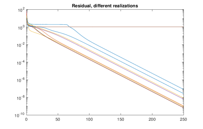
Figure 2: Evolution of the residual ($\|\mathscr{P}([\![\boldsymbol{A},\boldsymbol{B},\boldsymbol{H}]\!])-\boldsymbol{y}\|_{2}$) with respect to the number of cycles of ALS.

We use $N=30$ operating points generated randomly on the unit circle. We run Algorithm 1 for $10$ different starting points (i.i.d. Gaussian distributed), maximum $250$ iterations, and show the convergence plots in Fig. 2. We see that the algorithm converges linearly for all but one initialization, which is reasonable due to nonconvexity of the problem. For one of the realizations, the final residual is $\|\mathscr{P}([\![\boldsymbol{A},\boldsymbol{B},\boldsymbol{H}]\!])-\boldsymbol{y}\|_{2}=8.48\cdot 10^{-9}$, and the estimated factor $\widehat{\boldsymbol{A}}$ is (with the first row normalized to $1$ and shown with $4$ fractional digits of the mantissa),

$$\widehat{\boldsymbol{A}}=\begin{bmatrix}1&1\\ -1.3333-i0.8305\cdot 10^{-8}&0.3333+i0.4203\cdot 10^{-9}\\ 0.3333-i0.2210\cdot 10^{-8}&0.4999+i0.7007\cdot 10^{-10}\\ \end{bmatrix},$$

which is complex-valued, but recovers quite accurately the true ${\boldsymbol{A}}$ (the same holds for $\boldsymbol{B}$, not shown here).

In order to illustrate the reconstruction of the nonlinearities, instead of solving the least squares problem in Algorithm 1, we apply the idea similar the visualization of nonlinearities in Dreesen et al. (2015). In fact, the elements of $\boldsymbol{H}$ can be combined in such a way to yield the values of the derivatives of $g_{\ell}(\cdots)$ at the points $a(\mu_{k})$. We perform polynomial regression for degree $2$, take the real parts and obtain the following polynomials (with leading coefficient normalized to $1$), rounded to the $4$ fractional digits

$$h_{1}(t)=t^{2}-0.2222t,\quad h_{2}(t)=t^{2}-0.2.$$

after inspecting (10), we obtain that these are (up to numerical errors) the derivatives of the original nonlinearities, (i.e., $h_{1}(t)=\alpha g_{1}^{\prime}(t)$, $h_{2}(t)=\alpha g_{2}^{\prime}(t)$ with $\alpha=9$).

6 Conclusion

We developed a novel promising algorithm for identification of Wiener-Hammerstein systems from Volterra kernels. Our approach has the following advantages:

• It is based on tensor recovery, rather than CPD with structured factors, and can be solved with a simple alternating least squares scheme.

• It does not need all the coefficients of the Volterra kernels to be estimated: we just need to compute contractions with Vandermonde-structured vectors for a fixed number of operating points.

Furthermore, we believe that our method may have an interesting interpretation from the frequency-domain identification perspective. Note that the operating points that we use are typically taken on the unit circle, i.e., an operating point is chosen as $\mu_{k}=e^{2\pi i\omega_{k}}$. Viewed from a frequency-domain point of view (Pintelon and Schoukens, 2012), contraction of Volterra kernels with Vandermonde-structured vectors is somewhat similar to an “excitation” of the first-order derivative at a frequency $\omega_{k}$. However, for such an interpretation, we would potentially need to consider the framework of the Volterra kernel identification with complex valued inputs (Bouvier et al., 2019).

This research was supported by the ANR (Agence Nationale de Recherche) grant LeaFleT (ANR-19-CE23-0021); KU Leuven start-up-grant STG/19/036 ZKD7924; KU Leuven Research Fund; Fonds Wetenschappelijk Onderzoek - Vlaanderen (EOS Project 30468160 (SeLMA), SBO project S005319N, Infrastructure project I013218N, TBM Project T001919N, Research projects G028015N, G090117N, PhD grants SB/1SA1319N, SB/1S93918, and SB/151622); Flemish Government (AI Research Program); European Research Council under the European Union’s Horizon 2020 research and innovation programme (ERC AdG grant 885682). P. Dreesen is affiliated to Leuven.AI – KU Leuven institute for AI, Leuven, Belgium. Part of this work was performed while P. Dreesen and M. Ishteva were with Dept. ELEC of Vrije Universiteit Brussel, and P. Dreesen was with CoSys-lab at Universiteit Antwerpen, Belgium. The authors would like to thank the three anonymous reviewers for their useful comments that helped to improve the presentation of the results.

References

- Birpoutsoukis et al. (2017) Birpoutsoukis, G., Marconato, A., Lataire, J., and Schoukens, J. (2017). Regularized nonparametric Volterra kernel estimation. Automatica, 82, 324–327.
- Bouvier et al. (2019) Bouvier, D., Hélie, T., and Roze, D. (2019). Phase-based order separation for Volterra series identification. International Journal of Control. 10.1080/00207179.2019.1694175.
- Comon (2014) Comon, P. (2014). Tensors : A brief introduction. IEEE Signal Processing Magazine, 31(3), 44–53.
- Comon et al. (2009) Comon, P., Luciani, X., and De Almeida, A.L. (2009). Tensor decompositions, alternating least squares and other tales. Journal of Chemometrics, 23(7-8), 393–405.
- Dreesen and Ishteva (2021) Dreesen, P. and Ishteva, M. (2021). Parameter estimation of parallel Wiener-Hammerstein systems by decoupling their Volterra representations. In 19th IFAC Symposium on System Identification (SYSID 2021).
- Dreesen et al. (2015) Dreesen, P., Ishteva, M., and Schoukens, J. (2015). Decoupling multivariate polynomials using first-order information and tensor decompositions. SIAM Journal on Matrix Analysis and Applications, 36(2), 864–879.
- Dreesen et al. (2017) Dreesen, P., Westwick, D.T., Schoukens, J., and Ishteva, M. (2017). Modeling Parallel Wiener-Hammerstein Systems Using Tensor Decomposition of Volterra Kernels, volume 10169 of Lecture Notes on Computer Science, 16–25. Springer International Publishing, Cham.
- Dreesen et al. (2018) Dreesen, P., De Geeter, J., and Ishteva, M. (2018). Decoupling multivariate functions using second-order information and tensors. In Y. Deville, S. Gannot, R. Mason, M.D. Plumbley, and D. Ward (eds.), Latent Variable Analysis and Signal Separation, 79–88. Springer International Publishing, Cham.
- Giri and Bai (2010) Giri, F. and Bai, E. (2010). Block-oriented Nonlinear System Identification. Lecture Notes in Control and Information Sciences. Springer.
- Hollander (2017) Hollander, G. (2017). Multivariate polynomial decoupling in nonlinear system identification. Ph.D. thesis, Vrije Universiteit Brussel.
- Katayama (2005) Katayama, T. (2005). Subspace Methods for System Identification. Springer.
- Kibangou and Favier (2007) Kibangou, A. and Favier, G. (2007). Toeplitz–Vandermonde matrix factorization with application to parameter estimation of Wiener–Hammerstein systems. IEEE Signal Processing Letters, 14, 141–144.
- Kolda and Bader (2009) Kolda, T. and Bader, B. (2009). Tensor decompositions and applications. SIAM Review, 51(3), 455–500.
- Ljung (1999) Ljung, L. (1999). System identification. Wiley.
- Palm (1979) Palm, G. (1979). On representation and approximation of nonlinear systems. Biological Cybernetics, 34(1), 49–52.
- Pintelon and Schoukens (2012) Pintelon, R. and Schoukens, J. (2012). System Identification: A Frequency Domain Approach. Wiley, 2nd edition.
- Schetzen (1980) Schetzen, M. (1980). The Volterra and Wiener Theories of Nonlinear Systems. Wiley, New York.
- Schoukens and Tiels (2017) Schoukens, M. and Tiels, K. (2017). Identification of block-oriented nonlinear systems starting from linear approximations: A survey. Automatica, 85, 272–292.
- Usevich (2014) Usevich, K. (2014). Decomposing multivariate polynomials with structured low-rank approximation. In 21th International Symposium on Mathematical Theory of Networks and Systems (MTNS 2014).
- Van Mulders et al. (2014) Van Mulders, A., Vanbeylen, L., and Usevich, K. (2014). Identification of a block-structured model with several sources of nonlinearity. In 2014 European Control Conference (ECC), 1717–1722. 10.1109/ECC.2014.6862455.
- Westwick et al. (2017) Westwick, D., Ishteva, M., Dreesen, P., and Schoukens, J. (2017). Tensor factorization based estimates of parallel Wiener Hammerstein models. In Proc. 20th IFAC World Congress (IFAC 2017), volume 50(1) of IFAC-PapersOnLine, 9468–9473. Toulouse, France.