Constraints on ultracompact minihalos from the extragalactic gamma-ray background observation

Abstract

Ultracompact minihalo (UCMH) is a special type of dark matter halo with a very steep density profile which may form in the early universe seeded by an overdense region or a primordial black hole. Constraints on its abundance give valuable information on the power spectrum of primordial perturbation. In this work, we update the constraints on the UCMH abundance in the universe using the extragalactic gamma-ray background (EGB) observation. Comparing to previous works, we adopt the updated Fermi-LAT EGB measurement and derive constraints based on a full consideration of the astrophysical contributions. With these improvements, we place constraints on UCMH abundance 1-2 orders of magnitude better than previous results. With the background components considered, we can also attempt to search for possible additional components beyond the known astrophysical contributions.

I Introduction

The extragalactic gamma-ray background (EGB) is the total contribution of gamma-ray integrated flux from all objects in the history of the extragalactic universe, and was first detected by the SAS-2 satellite Fichtel et al. (1978); Thompson and Fichtel (1982) and subsequently measured by the Energetic Gamma Ray Experiment Telescope (EGRET) Osborne et al. (1994); Sreekumar et al. (1998); Willis (2002). Better measurements on EGB were achieved by the Large Area Telescope (LAT) Atwood et al. (2009) instrument installed on the Fermi satellite Abdo et al. (2010); Ackermann et al. (2015). The integrated flux of Fermi-LAT observation above 100 MeV is $1.29\pm 0.07\times 10^{-5}\,{\rm ph/cm^{2}/s/sr}$ (Model B of Ackermann et al. (2015)), consistent with those of EGRET, $1.14\pm 0.05\,{\rm ph/cm^{2}/s/sr}$ Strong et al. (2004). The latest Fermi-LAT observation shows that a power law function with an exponential cutoff ($dN/dE=I_{100}({E}/{\rm 100\,MeV})^{-\gamma}\exp(-{E}/{E_{\rm cut}})$) can well describe the EGB spectrum Ackermann et al. (2015), with spectral index of $\gamma=2.28\pm 0.01$ and cutoff energy of $E_{\rm cut}=267\pm 37\,{\rm GeV}$ (model B of Ackermann et al. (2015)).

Fermi-LAT also provides more accurate observations of extragalactic sources Acero et al. (2015); Abdollahi et al. (2020), allowing for a better understanding of the compositions of the EGB. It has been shown that the extragalactic gamma-ray background is mainly contributed by Blazars, radio galaxies (RG) and star-forming galaxies (SFG) Inoue (2011); Ackermann et al. (2012); Zeng et al. (2013); Ajello et al. (2014); Di Mauro et al. (2014); Ajello et al. (2015); Qu et al. (2019); Zeng et al. (2021); Roth et al. (2021). Most of extragalactic sources detected in the Fermi sky are Blazars Ajello et al. (2020a), which can be further classified into two subclasses, BL Lac and flat-spectrum radio quasars (FSRQs) Padovani (1997). Blazars could emit gamma rays through inverse Compton scattering (ICS) and / or hadronic processes and their contribution to EGB has been widely discussed Zeng et al. (2013); Ajello et al. (2014, 2015); Qu et al. (2019); Zeng et al. (2021). Radio galaxies, although with lower gamma-ray luminosity for individual sources, are more numerous in the whole sky. The contribution of RGs to the EGB can be studied via the correlation between radio and gamma-ray luminosities Inoue (2011); Di Mauro et al. (2014). The $\gamma$-ray radiation of SFG arises from the decay of neutral mesons produced in the inelastic interaction of cosmic rays with the interstellar medium and interstellar radiation field Ackermann et al. (2012); Ajello et al. (2020b). Above 100 MeV, RG and SFG each contributes about 10-30% of the observed photon flux of EGB, while blazars contribute about $\sim 50\%$ Ajello et al. (2015). In addition, the contributions to EGB from other sources or processes include gamma-ray bursts (GRB) Casanova et al. (2007), pulsars at high galactic latitudes Faucher-Giguère and Loeb (2010), inter-galactic shocks Loeb and Waxman (2000); Totani and Kitayama (2000), cascade processes of high energy cosmic rays Dar and Shaviv (1995), and so on.

Except for the aforementioned components, another source that may contribute to EGB is the dark matter (DM) Abazajian et al. (2010); Ajello et al. (2015); Ando and Ishiwata (2015); Di Mauro and Donato (2015); Fermi LAT Collaboration (2015); Liu et al. (2017); Blanco and Hooper (2019); Arbey et al. (2020). The existence of DM has been confirmed by many astronomical and cosmological observations, and it is likely to account for $\sim$26% of the total energy density of the Universe Planck Collaboration et al. (2016). DM has the potential to emit gamma-ray signals through annihilation or decay. The flux depends on the interaction cross-section of DM particles and the DM abundance Ginzburg and Syrovatskii (1964); Ricotti and Gould (2009a). Therefore, the DM properties (cross section or abundance) can be constrained by requiring the expected flux not higher than the actual measurements of the EGB spectrum.

In this work, we will focus on a particular DM halo model, i.e. ultracompact minihalos (UCMH) Ricotti and Gould (2009b); Scott and Sivertsson (2009); Yang et al. (2011a, b); Yang (2020), and constrain their abundance in the Universe with the EGB observation. The UCMH is characterized by a very steep density profile ($\rho\propto r^{-9/4}$). If DM consists of Weakly Interacting Massive Particles (WIMPs), the UCMHs will be gamma-ray emitters due to the DM annihilation within them and the profile makes them have high expected gamma-ray flux compared to the normal DM halo (e.g. NFW Navarro et al. (1997), Einasto Springel et al. (2008)). Constraints on the abundance of UCMHs or primordial black hole (PBHs) may provide valuable information on the power spectrum of the primordial perturbulation at small scale Josan and Green (2010); Bringmann et al. (2012); Aslanyan et al. (2016); Nakama et al. (2018).

In idealized cases, the UCMH can form in the early universe when the primordial density perturbations are between 10^-3 and 0.3 (a PBH will be produced if the amplitude of the perturbation is $\delta>0.3$ Carr et al. (2010)). However it has been shown that the postulated steep inner profile can not appear in realistic simulations since the required initial conditions (self-similarity, radial infall, isolation, etc) for forming UCMHs can only be satisfied in idealized cases Delos et al. (2018a, b); Adamek et al. (2019). Alternatively, PBHs formed in the early Universe can accret DM particles due to gravity and form UCMHs (a mixed WIMP-PBH dark matter model) Adamek et al. (2019); Yang (2020). In this work, we give constraints from an observational aspect, regardless of the exact mechanism of UCMH formation. Our constraints on the UCMH abundance can be directly converted into constrants on the PBHs in the mixed model Yang (2020). Furthermore, the derived constraints are also valid for the mini-spike around a astrophysical black hole Belikov and Silk (2014); Lacroix and Silk (2018); Cheng et al. (2020); Xia et al. (2021).

Comparing to previous works Yang et al. (2011a); Yang (2020), our studies contain the following improvements. We use the updated Fermi-LAT EGB observation to perform the analysis. In addition, in the previous works of limiting the abundance of UCMH with the EGB observations Yang et al. (2011a); Yang (2020); Nakama et al. (2018), they usually used the inclusive energy spectrum to provide relatively conservative constraints without considering the astrophysical components. We will alternatively derive restrictions based on a full consideration of the astrophysical contributions to obtain more realistic (though not that conservative) results. With the background components considered, we can also attempt to search for possible signals / additional components beyond the background. Another motivation for our study of UCMH is that this type of objects was recently suggested to be able to better (compared to the traditional density profiles, e.g. NFW, Einasto) interpret the tentative 1.4 TeV $e^{+}e^{-}$ excess of DAMPE (Dark Matter Particle Explorer) DAMPE Collaboration et al. (2017); Huang et al. (2018); Zhao et al. (2019); Cheng et al. (2020). We therefore examine whether such a probability can accommodate the abundance upper limits derived from the EGB observation.

Through out this papper, we use the cosmological parameters from Planck2015 Planck Collaboration et al. (2016), i.e. $\Omega_{m}=0.31$, $\Omega_{\Lambda}=0.69$ and $H_{0}=67.74\,{\rm km\,Mpc^{-1}s^{-1}}$.

II Methed

II.1 The model expected gamma-ray signal from a single UCMH

UCMHs are growing spherical DM halos which are seeded by an overdense region in the early universe with initial density perturbations greater than 0.01% (or alternatively seeded by a PBH). The mass of UCMHs $M_{u}$ depends on their formation time and can be described as Ricotti and Gould (2009b); Scott and Sivertsson (2009):

$$M_{u}(z)=\delta_{m}\left(\frac{1+z_{\rm eq}}{1+z}\right)$$ (1)

where $\delta_{m}$ is the mass of the perturbation at the redshift of matter-radiation equality ($1+z_{\rm eq}\approx 3260$). Since the accretion will be prevented after $z=10$, we assume the UCMHs stoped growing at $z=10$, i.e. $M(z<10)=M(z=10)$ Scott and Sivertsson (2009). Compared to the amplitude of perturbations seen in CMB observation ($\sim 10^{-5}$), the requred value for forming UCMH ($>10^{-3}$) is large. The non-Gaussian perturbations at phase transitions can enhance the amplitudes at small scale, therefore the UCMHs are more likely borned at the epoches of phase transitions. The UCMHs produced at three phase transitions are usually considered in literature Scott and Sivertsson (2009); Josan and Green (2010); Yang et al. (2011a, b): electroweak symmetry breaking, the QCD confinement and $e^{+}e^{-}$ annihilation. The $\delta_{m}$ for (QCD, EW, $e^{+}e^{-}$) epoches are $\delta_{m,{\rm\{EW,QCD,e+e-\}}}$={$5.6\times 10^{-19}$, $1.1\times 10^{-9}$, 0.33}$\,{\rm M_{\odot}}$ Scott and Sivertsson (2009) and the current masses of UCMHs are $M_{u}(0)$= {$1.6\times 10^{-7}$, $0.2$, $1.2\times 10^{5}$}$\,{\rm M_{\odot}}$, respectively. In fact, the chossen of the $\delta_{m}$ does not affect the predicted EGB spectrum of UCMH Yang et al. (2011a).

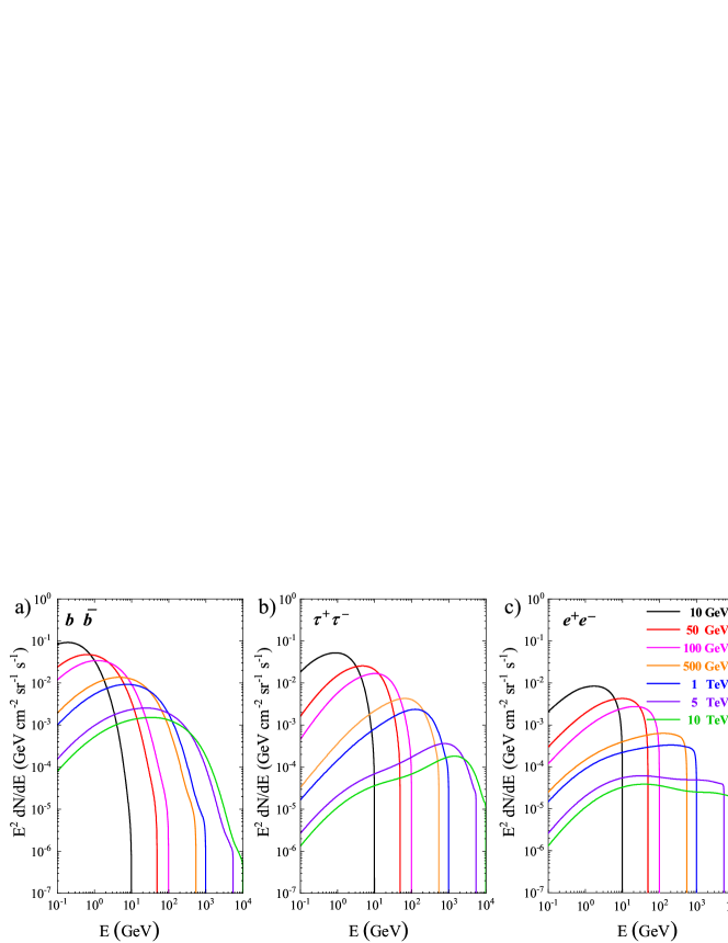
Figure 1: The model-predicted EGB spectra from UCMHs ($f_{u}=1$) for different channels and DM masses. The sharp cutoff at high energies close to $M_{\chi}$ could be a characteristic signature for DM search.

UCMHs are predicted to form by the secondary infall of DM onto PBHs or initial DM overdensity produced by the primordial density perturbation. The DM particles within the overdense region initially have an extremely small velocity dispersion. UCMHs thus form via a spherically symmetric gravitational collapse (pure radial infall). According to the secondary infall theory Fillmore and Goldreich (1984); Bertschinger (1985), the UCMHs will develop a self-similar power-law density profile $\rho\propto r^{-9/4}$. Such a steep profile is supported by both analytical solution Fillmore and Goldreich (1984); Bertschinger (1985) and (idealized) N-body simulations Vogelsberger et al. (2009); Ludlow et al. (2010); Delos et al. (2018a). Normalizing the $\rho(r)$ to make it have a halo mass of $M_{u}(z)$ within the truncated radius $R_{u}(z)$ gives the density profile of Ricotti and Gould (2009b); Scott and Sivertsson (2009)

$$\rho_{u}(r,z)=\frac{3f_{\chi}M_{u}(z)}{16\pi R_{u}(z)^{{3}/{4}}r^{{9}/{4}}}$$ (2)

where $f_{\chi}=\Omega_{\chi}/(\Omega_{b}+\Omega_{\chi})\approx 0.83$ Planck Collaboration et al. (2016). The profile truncated at a halo radius Scott and Sivertsson (2009)

$${R_{u}(z)}=0.019\left(\frac{1000}{z+1}\right)\left(\frac{M_{u}(z)}{\mathrm{M}_{\odot}}\right)^{{1}/{3}}{\rm pc}.$$ (3)

Due to the DM annihilation, for the most inner region of the halo ($r<r_{\rm cut}$) the density is set to Ullio et al. (2002)

$$\rho_{\max}(z)=\frac{m_{\chi}}{\langle\sigma v\rangle\left(t(z)-t_{i}\right)}$$ (4)

where $m_{\chi}$ is the mass of DM particle, $\langle\sigma v\rangle$ the annihilation cross section, and $t(z)$ is the age of the Universe at redshift $z$. The $r_{\rm cut}$ is determined by requiring the $\rho_{\rm max}=\rho(r_{\rm cut})$.

If DM consists of WIMPs, it can produce gamma rays through annihilation or decay. In this work, we mainly concern on the annihilation DM. The expected gamma-ray flux emitted from a single UCMH can be expressed as

$$F(E)=\frac{1}{4\pi}\frac{\langle\sigma{v}\rangle}{2m_{\chi}^{2}}\frac{dN_{\gamma}}{dE}\times\iint_{\rm los}\rho_{u}^{2}(r)dsd\Omega$$ (5)

where ${dN_{\gamma}}/{dE}$ is the photon yield per annihilation, which is calculated using PPPC4DMID Cirelli et al. (2012).

II.2 Extragalactic $\gamma$-ray background from UCMHs

For UCMHs with monochromatic mass function, the differential EGB energy spectrum contributed by UCMHs is expressed as Bergström et al. (2001); Ullio et al. (2002); Yang (2020):

$$\frac{d\phi_{\gamma}}{dE}=\frac{f_{u}\,\rho_{c,0}}{M_{u}(0)}\frac{c}{8\pi}\frac{\langle\sigma v\rangle}{m_{\chi}^{2}}\int_{0}^{z_{up}}dz\frac{e^{-\tau(E,z)}}{H(z)}\frac{dN_{\gamma}}{dE}(E^{\prime},z)\int\rho_{u}^{2}(r,z)dV$$ (6)

where $f_{u}$ is the present abundance of UCMHs (in terms of the fraction of the critical density $\rho_{c,0}$), $E^{\prime}=E(1+z)$ is the photon energy at redshift $z$, $E$ is the observed photon energy, the $z_{\mathrm{up}}=m_{\chi}/E-1$ is the maximal redshift that a UCMH can contribute photons of energy $E$. For the DM annihilation cross section, we adopt the thermal relic value ${\langle\sigma v\rangle}=3\times 10^{-26}\mathrm{cm}^{3}/\mathrm{s}$ Steigman et al. (2012); and for the Hubble parameter $H(z)=H_{0}\sqrt{\Omega_{M}(1+z)^{3}+\Omega_{\Lambda}}$, we use the cosmological parameters from Planck2015 Planck Collaboration et al. (2016). The $\tau$($E$,$z$) in Eq.(6) is the optical depth, for which we consider the EBL absorption only and can be approximated by $\tau(E,z)\sim z/3.3\,({E}/{10\,\mathrm{GeV}})^{0.8}$ Bergström et al. (2001). We use the approximation expression (rather than the models of e.g. Domínguez et al. (2011); Inoue et al. (2013)) for better obtaining $\tau$ at high redshift (e.g. $z>10$).

In addition to the prompt gamma-ray emission, DM annihilation can produce energetic electrons/positrons, which generate gamma rays through inverse Compton scattering (ICS) off background radiation field. In this work, we only consider the prompt gamma rays from DM annihilation but neglecting the secondary IC component. Tighter constraints are expected with the IC contribution included. The contribution to the EGB from normal halos is also ignored, since it has been shown that the inclusion of them hardly affect the results Yang et al. (2011a) due to the much lower annihilation rate therein. For the three typical channels $b\bar{b},\tau^{+}\tau^{-}$ and $\mathrm{e}^{+}\mathrm{e}^{-}$, we show the DM-induced EGB spectra with $f_{u}=1$ in Fig.1.

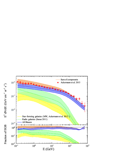
Figure 2: The EGB spectrum observed by Fermi-LAT (red points) Ackermann et al. (2015) together with the predicted astrophysical contributions from blazars (blue band) Ajello et al. (2015), radio galaxies (green band) Inoue (2011) and star-forming galaxies (yellow band) Ackermann et al. (2012). All the components have not been renomalized through the $\chi^{2}$ fitting, yet. The red band is the sum of all three components. The lower panel demonstrates the fraction of each astrophysical component contributing to the total EGB spectrum.

II.3 Astrophysical components of the extragalactic gamma-ray background

Compared with former researches on limiting UCMHs with EGB, one of the improvements is we consider the contributions to EGB from background astrophysical components. The previous works have shown that most of the EGB can be accounted for by the joint contributions of blazars (including both BL Lac objects and FSRQs), radio galaxies (RG) and star-forming galaxies (SFG). Above 100 MeV RG and SFG each contributes about 10-30% of the observed photon flux of EGB, while blazars contributes about $\sim 50\%$ Ajello et al. (2015). The luminosity functions of these source populations can be derived from the resolved gamma-ray sources (for blazar) or from the relations between radio/infrared and gamma-ray luminosities (for SFG and RG). The contribution from the unresolved extragalactic sources can then be estimated by extrapolating the luminosity function (LF). In this paper, we consider these three types of sources as well. For SFG and RG, we directly use the EGB spectrum (and corresponding uncertainties) presented in Ackermann et al. (2012) (MW model) and Inoue (2011). A newer result for the SFG contribution to the EGB has been reported in Ajello et al. (2020b). We also use the SFG spectrum in Ajello et al. (2020b) (the one based on the IR luminosity function of Gruppioni et al. (2013)) to test the main results of this paper and find that it only slightly affect the results since the SFG component accounts for merely $5\%$ of the total EGB. For blazars we employ the formalism and parameters in Ajello et al. (2014, 2015), which will be briefly re-introduced below.

The differential intensity (in unit of ${\rm ph\,cm^{-2}sr^{-1}s^{-1}GeV^{-1}}$) of the EGB contributed by the blazars with photon index ($1.0<\Gamma_{\gamma}<3.5$), redshift ($10^{-3}<z<6$) and gamma-ray luminosity ($10^{43}<L_{\gamma}<10^{52}$) can be computed by:

$$F_{\rm EGB}(E) =\int_{\Gamma_{\min}=1.0}^{\Gamma_{\max}=3.5}d\Gamma\int_{z_{\min}=10^{-3}}^{z_{\max}=6}dz\int_{L_{\gamma,\min}=10^{43}}^{L_{\gamma,\max}=10^{52}}dL_{\gamma}$$ (7)

$$\times\Phi\left(L_{\gamma},z,\Gamma\right)\cdot f(E)\cdot\frac{dV}{dzd\Omega}$$

where $dV/(dzd\Omega)$ is the differential comoving volume at redshift $z$, and the EBL modulated spectrum of blazars is

$$f(E;\Gamma,z,L_{\gamma})=K\left[\left(\frac{E}{E_{b}}\right)^{1.7}+\left(\frac{E}{E_{b}}\right)^{2.6}\right]^{-1}\cdot e^{-\tau(E,z)}$$

with $\log E_{b}({\rm GeV})\approx 9.25-4.11\Gamma$ and $K=L_{\gamma}/[4\pi d_{L}^{2}k\int Ef(E,K=1)dE]$, where $k$ is the $K$-correction term. For the optical depth term here we use the EBL model of Domínguez et al. (2011).

The $\Phi$ in Eq. (7) is the blazar LF, namely the number density of blazars at luminosity $L_{\gamma}$, redshift $z$ and spectral index $\Gamma$. We use the simplest pure density evolution (PDE) model of the LF, which reads

$$\Phi\left(L_{\gamma},z,\Gamma\right)=\Phi\left(L_{\gamma},z=0,\Gamma\right)\times e\left(z,L_{\gamma}\right)$$ (8)

where the luminosity function at redshift $z=0$ is

$$\Phi\left(L_{\gamma},z=0,\Gamma\right)=\frac{dN}{dL_{\gamma}dVd\Gamma}$$ (9)

$$\quad=\frac{A}{\ln(10)L_{\gamma}}\left[\left(\frac{L_{\gamma}}{L_{*}}\right)^{\gamma_{1}}+\left(\frac{L_{\gamma}}{L_{*}}\right)^{\gamma_{2}}\right]^{-1}\cdot e^{-0.5\left[\Gamma-\mu\left(L_{\gamma}\right)\right]^{2}/\sigma^{2}}.$$

The expressions of $e(z,L_{\gamma})$ and $\mu(L_{\gamma})$ can be found in Ajello et al. (2015).

We plot the model expected EGB spectra for blazar, RG and SFG together with the Fermi-LAT EGB measurements in Fig. 2. Also shown is the proportion of each component in the total observed EGB.

II.4 Limiting the abundance of UCMHs with the Fermi-LAT EGB observation

If the UCMHs exist in the Universe, they are another type of extragalactice gamma-ray emitters due to the DM annihialtaion Scott and Sivertsson (2009). The annihilation photons may contribute to the extragalactic gamma-ray background, it is practicable to limit the abundance of UCMHs with EGB observation. The latest EGB measurements at GeV energies are from the Fermi-LAT observation Ackermann et al. (2015). The Fermi-LAT Collaboration adopted three different Galactic foreground models to obtain the EGB spectrum. For our purpose they do not differ with each other significantly, and in this paper we use the foreground model B of Ackermann et al. (2015).

To compare the models with the observation, the $\chi^{2}$ fitting method is used. We first obtain the best-fit astrophysical components without the DM model included by minimizing

$$\chi^{2}= \sum_{i=1}^{N}\frac{\left(F_{i,{\rm obs}}-\bm{\alpha}_{1}F_{i,1}-\bm{\alpha}_{2}F_{i,2}-\bm{\alpha}_{3}F_{i,3}\right)^{2}}{\sigma_{i,{\rm obs}}^{2}}$$ (10)

$$+\sum_{j=1}^{3}\frac{\left(1-\bm{\alpha}_{i}\right)^{2}}{\delta_{j}^{2}}$$

where $F_{i,{\rm obs}}$ and the $\sigma_{i,{\rm obs}}$ are the EGB spectrum measured by the Fermi-LAT (see Table 3 of Ackermann et al. (2015)). The error bars $\sigma_{i,{\rm obs}}$ include the statistical uncertainty and systematic uncertainties from the effective area parameterization, as well as the CR background subtraction Ackermann et al. (2015). The systematic uncertainty related to the modeling of the Galactic foreground is not further included, which may vary the intensity by $+15\%/-30\%$. However, we adopt the EGB spectrum having the highest intensities among the three benchmark foreground models in Ackermann et al. (2015) (i.e. the FG model B), which would give relatively conservative constraints. The $F_{i,1}$ ,$F_{i,2}$ ,$F_{i,3}$ in Eq. (10) are the model-expected fluxes of the $i{-\text{th}}$ energy bin from blazar, RG and SFG, respectively, and the $\bm{\alpha}_{i}$ is a renormalization constant of each spectrum which is free to vary in the fit. The last term is introduced to ensure that the best-fit gamma-ray intensities do not deviate from their original values in the literature too much. The $\delta_{j}$ is determined by the uncertainty band of each component as demonstrated in Fig. 2 and we choose a mean value over all the energies.

Based on the best-fit astrophysical model, we add an additional UCMH component into the $\chi^{2}$ fit to constrain the UCMH abundance or search for possible signals. At this stage, the $\chi^{2}$ is defined as

$$\chi^{2}=\sum_{i=1}^{N}\frac{\left[F_{i,{\rm obs}}-\mathcal{A}F_{i,\rm astro}-f_{u}F_{i,\rm ucmh}\right]^{2}}{\sigma_{i,\rm obs}^{2}}$$ (11)

where $F_{i,\rm astro}$ is the sum of the best-fit astrophysical contributions in the above step, and $F_{i,\rm ucmh}$ is the flux from UCMHs as calculated by Eq. (6).

The best-fit chi-square value $\chi^{2}_{f_{u}}$ will change along with the given normalization parameter of the UCMH component. The chi-square difference is $\Delta\chi^{2}=\chi^{2}_{f_{u}}-\chi^{2}_{f_{u}=0}$ where $\chi^{2}_{f_{u}=0}$ is the minimum $\chi^{2}$ under the background-only model. Because for a fixed DM mass $M_{\chi}$, the UCMH model have 1 more additional parameter than the background model, the chi-square difference follows $\Delta\chi^{2}\sim\chi^{2}(1)$ Chernoff (1954). The variance of the $\chi^{2}$ by 2.71 corresponds to an upper limit of the abundece at 95% confidence level.

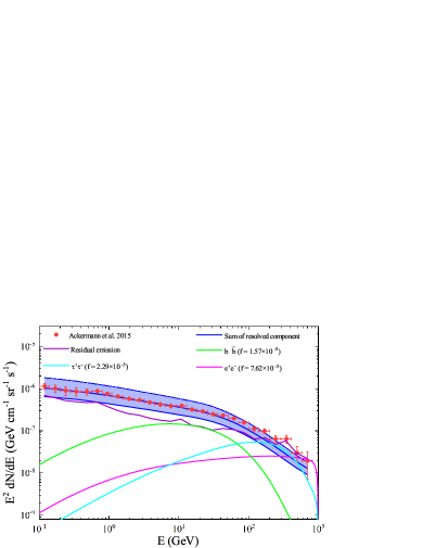
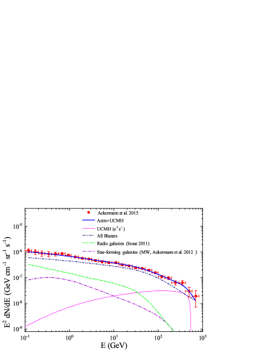
Figure 3: Left panel: The best-fit EGB spectrum without a DM component included (blue line and relevant uncertainty band). The purple line is the conservative residuals subtracting the best-fit astrophysical contributions (see the main text for details). Also shown are the DM spectra for 1 TeV DM for $b\bar{b}$ (green line), $\tau^{+}\tau^{-}$ (cyan line) and $\mathrm{e}^{+}\mathrm{e}^{-}$ (magenta line) channels, respectively. In this plot, the amplitude of the three components are determined by requiring not to exceed the residual emission (i.e. a demonstration of our conservative methods). Right panel: The best-fit total EGB spectrum containing the DM component (blue line) and the individual contributions.

III RESULT

The fitted renormalization parameters $\alpha_{i}$ for the three background components and the 1$\sigma$ uncertainties are summarized in Table 1 (benchmark row). For Blazar and SFG they are close to 1, while for RG a smaller renomalization parameter is required to fit the data. In Fig.3 we exhibit the best-fit background-only EGB spectrum as well as the corresponding conservative residuals (see below). Also shown are the spectra of UCMH with $M_{\chi}$=1 TeV in different annihilation channels, which are required not to exceed the residuals in the plot. We can see that below 50 GeV, the model match the data points well, while at energies of $>50$ GeV it slightly underestimates the observation.

According to the $\chi^{2}$ analysis (Eq. (11)), the upper limits on the UCMH abundance $f_{u}$ as a function of DM mass $M_{\chi}$ after containing astrophysical components in the fit are shown in Fig.4 for $b\bar{b}$, $\tau\tau$, $e^{+}e^{-}$ channels. For all three channels, we can place constraints on the abundance down to $\sim 3\times 10^{-6}$ in the range $M_{\chi}<100\,{\rm GeV}$, namely only $\lesssim 3\times 10^{-6}$ of the universe energy density could be in the form of UCMH, otherwise their predicted EGB emission will exceed the actual observation. For the $\tau^{+}\tau^{-}$ and $e^{+}e^{-}$ channels, the constraints become weaker as the $M_{\chi}$ is increased to $>$300 GeV. This is due to the existence of residuals at this high energy range (see Fig. 11) which may be accounted for by including a DM component (see Section IV.1).

Table 1: Best-fit results for the models with only astrophysical components.

Model	Balzar	RG	SFG	$\chi^{2}$
benchmark	$1.146^{+0.031}_{-0.031}$	$0.621^{+0.125}_{-0.125}$	$1.202^{+0.251}_{-0.251}$	19.359
MAGN	$1.001^{+0.029}_{-0.029}$	$0.723^{+0.091}_{-0.091}$	$1.489^{+0.251}_{-0.251}$	19.785
RG($\Gamma=2.11$)	$1.165^{+0.037}_{-0.037}$	$0.521^{+0.101}_{-0.101}$	$1.453^{+0.251}_{-0.251}$	24.288
SFG(PL)	$1.165^{+0.044}_{-0.044}$	$1.027^{+0.121}_{-0.121}$	$1.237^{+0.180}_{-0.180}$	19.558
SFG2020	$0.983^{+0.004}_{-0.004}$	$0.824^{+0.152}_{-0.152}$	$1.022^{+0.143}_{-0.143}$	21.685
$\tau=1.49$	$0.964^{+0.004}_{-0.004}$	$1.840^{+0.153}_{-0.153}$	$1.417^{+0.251}_{-0.251}$	11.443
$\gamma_{2}=1.35$	$0.710^{+0.018}_{-0.018}$	$1.180^{+0.127}_{-0.127}$	$1.309^{+0.251}_{-0.251}$	12.772

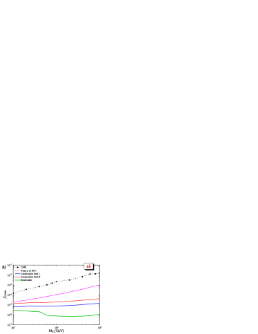
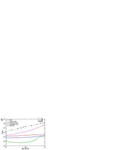
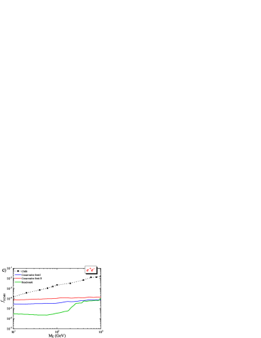
Figure 4: The constraints on the UCMH abundance in the Universe obtained through the EGB analysis in this work (solid lines). As a comparison, we also plot the previous constraints based on EGB (dashed) and CMB (dotted) observations Yang et al. (2011a). The three panels are for different annihilation channels as labeled in the plots.

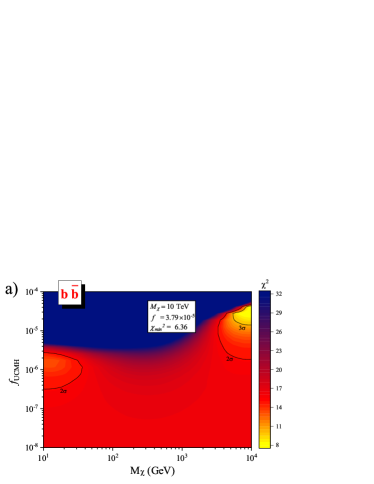
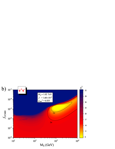
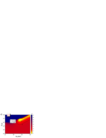
Figure 5: The $\chi^{2}$ maps as a function DM mass $M_{\chi}$ and UCMH abundance $f_{u}$ for three different annihilation channels. The brightest point with minimum $\chi^{2}$ corresponds to the best fit to the observation and the fitted parameters have been shown in the plots.

Compared with the previous results which are based on the 1-year Fermi-LAT EGB observation Yang et al. (2011a) (dashed line in Fig. 4), we can see that our constraints are about $1-2$ orders of magnitude better. The improvement is owing to the use of the updated EGB observation and subtracting the astrophysical contributions. The UCMH abundance $f_{u}$ in the universe can also be constrained by the CMB observation since in the early universe the particles emitted from the DM annihilation within UCMHs will influence the ionization and recombination before the structure formation Yang et al. (2011b, a). As a comparison, the CMB constraints with WMAP-7 data Yang et al. (2011a) are shown in the Fig. 4 (dotted line), which is however not as stringent as the EGB limits.

In addition, we use two other approaches to set more conservative limits. The most conservative one is obtained by using an inclusive EGB spectrum with no any background subtracted (I). Less conservative limits (II) are given by the following prescription. We define the upper bound of the error bars of the EGB measurements as $F_{i,\rm up}$, while for the model we use the lower bound of the uncertainty bands $F_{i,\rm low}$, and $F_{i,\rm res}=F_{i,\rm up}-F_{i,\rm low}$ is considered a conservative residual after subtracting the background. Namely, for the observation we adopt the maximal values under the $1\sigma$ range, and for the model-expected one we use the minimum. Requiring that the EGB from UCMHs does not exceed the $F_{i,\rm res}$ gives the limits on the UCMH abundance. As is shown, even with the most conservative approach, the results have improved greatly than that of Yang et al. (2011a), mainly due to the adoption of the new EGB observation.

IV DISCUSSIONS

IV.1 Searh for possible additional DM component

In contrast with previous analyses, we are able to search for possible UCMH signals in addition to the background components because the astrophysical contributions are considered in this work. The search is also based on the chi-square analysis of Eq. (11). A background model corresponds to $f_{u}=0$, while for the signal model $f_{u}$ is free to vary. Then the significance of the existence of a UCMH component is given by the chi-square difference $\Delta\chi^{2}$. According to Wilks’ theorem Chernoff (1954), the $\Delta\chi^{2}>9$ indicates the observed data rejecting the null model at a confidence level of $>3\sigma$, i.e. there may exist a possible signal. We scan for a series of DM masses with the EGB observation, and the related results are shown in Fig. 5.

In our analysis, we notice that the inclusion of a UCMH component improves the fit significantly. The test-statistic ($TS$) of the additional DM composition can be estimated by the difference of the minimum chi-square values between the following two cases: the fitting of only considering the astrophysical components, and that with the addition of a UCMH composition, namely $TS=\Delta\chi^{2}=\tilde{\chi}^{2}(f_{u}=0)-\tilde{\chi}^{2}$. The $\chi^{2}$ with tilde denotes the minimum value in the fit. The brightest points in Fig. 5 give the best-fit $M_{\chi}$ and $f_{u}$ parameters. We obtain the optimum DM masses of 10 TeV, 1.09 TeV and 0.55 TeV with TS of 13.0, 13.3 and 13.3 for $b\bar{b}$, $\tau\tau$ and $e^{+}e^{-}$, respectively. The TS$>9$ suggests existing a tentative signal.

Although such a tentative excess is interesting, it is difficult to reliably claim that it comes from UCMHs, given the large uncertainties in the modeling of astrophysical components. We here demonstrate that the uncertainties in the astrophysical models have a great impact on the obtained significance. We note that the fitting is improved mainly because the addition of a UCMH component compensates for the residuals in the high energy range (see Fig. 3 right for the demonstration). In light of this, we focus on some alternative models that can increase the high energy flux of the EGB spectrum. We do the following checks.

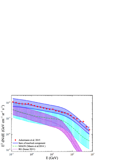
Figure 6: We compare the RG models of Di Mauro et al. (2014) and Inoue (2011). The RG model from Inoue (2011) has higher EGB flux at higher energies. The blue line is the best-fit adopting the model of Di Mauro et al. (2014) (DM component is not included).

Table 2: Best-fit parameters for the models with DM included.

Model	Channel	$f_{u}$	$M_{\chi}$	TS	$\chi^{2}$
Benchmark	$b\bar{b}$	$3.79\times 10^{-5}$	$10$	$12.99$	$6.36$
Benchmark	$\tau^{+}\tau^{-}$	$1.60\times 10^{-5}$	$1.09$	$13.32$	$6.03$
Benchmark	$e^{+}e^{-}$	$5.23\times 10^{-5}$	$0.55$	$13.27$	$6.08$
MAGN	$\tau^{+}\tau^{-}$	$1.50\times 10^{-5}$	$1.48$	$12.69$	$7.09$
RG/$\Gamma=2.11$	$\tau^{+}\tau^{-}$	$1.45\times 10^{-5}$	$1.48$	$14.78$	$9.50$
SFG/PL	$\tau^{+}\tau^{-}$	$1.85\times 10^{-5}$	$1.35$	$11.44$	$7.91$
SFG2020	$\tau^{+}\tau^{-}$	$1.87\times 10^{-5}$	$1.23$	$14.56$	$7.12$
$\tau=1.49$	$\tau^{+}\tau^{-}$	$1.17\times 10^{-5}$	$1.66$	$5.27$	$6.17$
$\gamma_{2}=1.35$	$\tau^{+}\tau^{-}$	$3.94\times 10^{-6}$	$2.23$	$5.05$	$7.72$

The reference Di Mauro and Donato (2015) has also searched for a probable DM component that could be hidden beneath the EGB. We note that they did not report the presence of a tentative additional component in the $>$100 GeV energy range. One difference between their work and ours is that for the RG component, they employ the energy spectrum of Di Mauro et al. (2014) instead of Inoue (2011) in our study. By comparison (Fig. 6), it can be found that the RG spectrum predicted by Di Mauro et al. (2014) has a higher energy flux than Inoue (2011) at energies greater than 100 GeV. We use the RG model of Di Mauro et al. (2014) to check our results with the models of the other components unchanged. The results reveal that even when the RG model is replaced, the fitting still gives a relatively high TS of the tentative DM component (see MAGN model in Table 1 & 2).

In addition, when modeling the SFG component, different assumptions of the average spectrum of the source population will lead to different EGB spectra of SFGs Ackermann et al. (2012). Our benchmark results adopt the MW model (i.e., assuming all SFGs are Milky Way-like), but at 100 GeV the PL model (all SFGs share the same spectrum as those detected by Fermi-LAT) is higher than the MW model by a factor of $\sim$10. We therefore examine the outcome of taking this SFG/PL model. Further, we notice that an updated result for the SFG contribution to the EGB has been reported in Ajello et al. (2020b). They derive the SFG spectrum based on the detection of 11 SFGs and the emission from unresolved SFGs with the 10-year Fermi-LAT data. We test the analysis with this SFG model and find results consistent with our benchmark ones. The related results are shown in the SFG2020 row of the two tables.

The large uncertainties in the LF parameters will induce a significant uncertainty of the predicted EGB spectrum. For RG we examine the spectral uncertainty introduced by the photon index parameter. We consider a harder photon index ($\Gamma=2.11$) of the source population in the luminosity function (see Fig. 4 of Inoue (2011)). The corresponding results are shown in Table 1 & 2 (labeled as RG/$\Gamma=2.11$). For the Blazar component, with the formalism described in Section II.3, we test the uncertainties associated with all 10 parameters of the PDE LF. The $\tau$ and $\gamma_{2}$ parameters are found to have the greatest influence on the obtained TS value when the parameter values are changed within their uncertainty range. The TS reduces to $\sim$5.3 and $\sim$5.1 for the $\tau=1.49$ and $\gamma_{2}=1.35$ models, respectively.

According to these test, we conclude that the results from the EGB analysis are currently subject to considerable uncertainty and we can not claim the presence of additional components despite obtaining a relatively high TS value.

IV.2 The UCMH contribution to the $e^{+}e^{-}$ energy density near the Earth

At last we discuss the implication of our constraints to the DAMPE 1.4 TeV excess. One of the most intriguing structrue displayed in the DAMPE $e^{+}e^{-}$ spectrum is the peak-like excess at $\sim$1.4 TeV with a significance of $\sim 3.7\sigma$ which may be caused by the monochromatic injection of electrons due to the DM annihilation within nearby DM halos DAMPE Collaboration et al. (2017); Yuan et al. (2017); Cao et al. (2018); Huang et al. (2018); Pan et al. (2018); Zhao et al. (2019). In the DM scenario, the DM annihilation is accompanied with production of gamma-ray photons. While the normal DM halo models (like NFW Navarro et al. (1997), Einasto Springel et al. (2008)) are challenged by the gamma-ray observations Ghosh et al. (2018); Belotsky et al. (2019), the DM annihilation within nearby UCMHs can provide a better interpretation to the excess Huang et al. (2018); Zhao et al. (2019); Cheng et al. (2020). Assuming that the local fraction of the DM in the form of UCMHs is identical to that in the whole universe, the above constraints can be used to exame the UCMH interpretation of the 1.4 TeV excess.

Here we especially consider the channel of $\chi\chi\rightarrow e^{+}e^{-}$. The number of electrons/positrons emitted per unit time and energy from a UCMH is

$$\frac{dN_{e}}{dEdt}=2R\cdot\delta(E-E^{\prime})$$ (12)

with $R$ the annihilation rate of the DM particles within the UCMH

$$R=\frac{\langle\sigma v\rangle}{2m_{\chi}^{2}}\int\rho^{2}\mathrm{~{}d}V.$$ (13)

We then have the injection rate of

$$Q(E,r)=\frac{{f_{u}}\rho_{\chi,\rm local}}{M_{u}(0)}\frac{dN_{e}}{dEdt}$$ (14)

where $\rho_{\chi,\rm local}=0.4\,{\rm GeV/cm^{3}}$ Catena and Ullio (2010) is the DM density near the location of the Earth. By solving the propagation equation of electrons one can obtain the energy density $\omega_{e}$ contributed by UCMHs for a given $f_{u}$. The narrow peak of the tentative exess requires the distance of the source is within $d$=0.3kpc for avoiding the widden of the peak due to cooling effect Yuan et al. (2017); Huang et al. (2018). Assuming the DM density of the field halo does not vary a lot within the region of propagation length (i.e. assuming the UCMHs distributed evenly near the Earth), we can reasonably neglect the diffusion term, and the number density of the electrons provided by UCMHs can be approximated by

$$\frac{dn_{e}}{dE}=\frac{1}{b(E)}\int_{E}^{\infty}Q\left(E^{\prime},r\right)dE^{\prime},$$ (15)

where the $b(E)\approx b_{2}(E/{\rm GeV})^{2}$ is the electron cooling rate, for which we consider only the synchrotron and ICS losses $b_{2}=1.0\times 10^{-16}\,{\rm GeV/s}$ Atoyan et al. (1995); Yuan et al. (2017).

The measured energy density of the 1.4 TeV peak is estimated to be about $1.2\times 10^{-18}\,{\rm erg\,cm^{-3}}$ Yuan et al. (2017). However, using Eq. (15) and the upper limits of the UCMH abundance in Fig. 4, we obtain an upper limits of the energy density of $\omega_{\rm up}\sim 6.25\times 10^{-19}\,{\rm erg/cm^{3}}$ for the ${e}^{+}{e}^{-}$ channel. This indicates that the UCMHs formed in the transition epoches with a density profile of $\gamma=-9/4$ is hard to interpret the DAMPE 1.4 TeV excess if the UCMH abundance near the Earth is the same as that in the whole universe. It has also been shown that such type ($\gamma=-9/4$) of UCMH is not supported by the realistic simulations Delos et al. (2018a, b); Adamek et al. (2019). To still use UCMH to account for the 1.4 TeV excess, possible solution is that the UCMHs are in the form of $\gamma=-3/2$ as expected by the simulations. The shallower density profile reduces the annihilation rate in the UCMHs, making the upper limits of the abundance deduced from the EGB observation much weaker. Note that the $\gamma=-3/2$ UCMHs could also behave as point-like sources in the Fermi-LAT gamma-ray sky Cheng et al. (2020), and would not be constrained by the gamma-ray observation. Another posibility is the UCMH abundance near the Earth is higher than the average value in the whole universe.

V summary

In this work, we revisit the analysis of constraining the UCMH abundance with EGB observations, using the latest measurements at 0.1-820 GeV energies by Fermi-LAT. Except for the use of updated data, another improvement of this work is that we take into account the astrophysical contributions in the EGB and subtract them before setting the constraints in order to obtain more strict limits on the abundance. With these improvements, we find that our results are 1-2 orders of magnitude better than previous. Even adopting a conservative method of using the inclusive EGB spectrum as Yang et al. (2011a), our results are substantially stronger due to the use of the new EGB observation Ackermann et al. (2015). Thus, the constraints presented in the work are currently the most serious ones for the UCMHs with monochromatic mass function. Though some $N$-body simulations do not support the existence of UCMHs, our results can also apply to the dressed PBH Adamek et al. (2019); Yang (2020).

In addition to deriving constraints, we also search for possible DM components after subtracting the astrophysical contributions. We find that in our benchmark model (see Table 2), the $\chi^{2}$ analysis shows that the significance of existing a UCMH component reaches $3.6\sigma$ (i.e., ${\rm TS}=13.3$) for the $\tau^{+}\tau^{-}$ channel. For $b\bar{b}$ and $e^{+}e^{-}$, the TS values are 13.0 and 13.3, respectively. However, we point out that the uncertainty of the astrophysical models is large and it is hard to claim the existence of an additional component at present. The TS value can be reduced to as low as $\sim 5.3$ if we change the astrophysical models. Observing more resolved extragalactic sources in the future with next generation gamma-ray telescopes (especially for the SFG and RG components) will be helpful to better determine the gamma-ray luminosity function of these source classes and is crucial for the better determination of whether existing additional components in the EGB.